Abstract
This study aims to enhance the accuracy and interpretability of flood susceptibility mapping (FSM) in Seoul, South Korea, by integrating automated machine learning (AutoML) with explainable artificial intelligence (XAI) techniques. Ten topographic and environmental conditioning factors were selected as model inputs. We first employed the Tree-based Pipeline Optimization Tool (TPOT), an evolutionary AutoML algorithm, to construct baseline ensemble models using Gradient Boosting (GB), Random Forest (RF), and XGBoost (XGB). These models were further fine-tuned using Bayesian optimization via Optuna. To interpret the model outcomes, SHAP (SHapley Additive exPlanations) was applied to analyze both the global and local contributions of each factor. The SHAP analysis revealed that lower elevation, slope, and stream distance, as well as higher stream density and built-up areas, were the most influential factors contributing to flood susceptibility. Moreover, interactions between these factors, such as built-up areas located on gentle slopes near streams, further intensified flood risk. The susceptibility maps were reclassified into five categories (very low to very high), and the GB model identified that approximately 15.047% of the study area falls under very-high-flood-risk zones. Among the models, the GB classifier achieved the highest performance, followed by XGB and RF. The proposed framework, which integrates TPOT, Optuna, and SHAP within an XAI pipeline, not only improves predictive capability but also offers transparent insights into feature behavior and model logic. These findings support more robust and interpretable flood risk assessments for effective disaster management in urban areas.
1. Introduction
Flooding remains one of the most devastating natural hazards globally, leading to significant disruptions in infrastructure, economies, and human lives. The situation is particularly critical in densely populated metropolitan areas such as Seoul, South Korea, where rapid urbanization and climate change have amplified both the frequency and intensity of flood events [1]. In this context, accurate flood susceptibility mapping (FSM) has become a vital tool for disaster risk reduction and urban resilience planning [2]. Physically based hydrologic and hydrodynamic models have been widely used to simulate flood dynamics. However, these approaches often require extensive input data and computational resources. As a complementary alternative, data-driven models offer greater flexibility in capturing complex, nonlinear relationships among environmental and anthropogenic factors, particularly in data-sparse urban settings [3].
Recent advances in machine learning (ML) offer a promising alternative for modeling flood risks, as ML algorithms can automatically learn patterns from data without explicit rule-based programming. A wide range of ML techniques has been employed for flood prediction and susceptibility assessment. Among these, soft computing and statistical learning models have gained popularity in recent years. Decision-tree-based algorithms such as random forest [4,5], artificial neural networks (ANNs) [6,7,8], support vector machines (SVMs) [9,10,11], gradient boosted tree (GB) [12] and logistic regression (LR) models [13] have all shown promise in capturing complex relationships between environmental variables and flood events. In addition to these methods, the frequency ratio (FR) model, one of the simplest statistical approaches, has been frequently used to identify correlations between flood occurrences and related conditioning factors [14,15]. For more comprehensive evaluations, researchers have integrated numerical modeling and multi-criteria decision analysis techniques such as the analytic hierarchy process (AHP) [16,17]. Moreover, some studies have adopted hydraulic simulations and developed thematic hazard maps by combining geophysical field surveys with GIS [18,19] and remote sensing technologies [20,21]. However, deploying these models in practice often requires meticulous tuning of hyperparameters and pipeline structures such as metaheuristic [22,23,24] and evolutionary algorithms [25,26], which can be time-consuming and prone to subjective bias. To address this, AutoML frameworks have gained traction [27,28]. Among them, the TPOT uses the genetic algorithm to evolve entire ML pipelines by simulating evolutionary processes [29]. While TPOT offers structural flexibility and automation, it also presents challenges in reproducibility and transparency due to its stochastic nature. Alternatively, Optuna leverages Bayesian optimization via the Tree-structured Parzen Estimator (TPE) to fine-tune hyperparameters within a user-defined pipeline. Although Optuna requires a fixed model architecture, its deterministic and scalable design makes it highly suitable for domains like FSM, where domain knowledge often informs model structure.
In parallel, the emergence of XAI has highlighted the importance of model interpretability in geospatial and environmental modeling [30]. While many ML models excel in predictive performance, their black-box nature often limits practical utility and stakeholder trust. This study addresses that concern by employing SHAP, a unified framework based on cooperative game theory, to quantify the contribution of each input feature to model predictions. SHAP supports both global and local interpretability, enabling not only the identification of dominant flood-driving factors but also the dissection of individual predictions. Furthermore, Optuna’s built-in visualization tools—such as optimization history, parameter importance plots, and slice plots—provide additional insights into the internal logic of the hyperparameter tuning process, enhancing transparency throughout the model development lifecycle.
This study presents a comparative evaluation of TPOT and Optuna as representative AutoML approaches for flood susceptibility assessment in Seoul, with a focus on balancing predictive performance and interpretability. By integrating SHAP-based model explanations and Optuna’s visual diagnostics, the proposed methodology aims to enhance both model accuracy and transparency. The specific objectives of this study are threefold:
- (1)
- To valuate and compare evolutionary and Bayesian optimization strategies in the context of real-world flood prediction.
- (2)
- To examine the trade-offs between automated and expert-driven pipeline design.
- (3)
- To generate spatially explicit insights into flood susceptibility using explainable ML tools.
Through this integrative approach, this study contributes to the growing body of research on AI-driven disaster risk modeling and demonstrates how AutoML and XAI can be effectively combined to support interpretable and actionable decision-making.
2. Study Area
This study focuses on Seoul, the capital and largest metropolis of South Korea, geographically located between 37.41° and 37.72°N latitude and between 126.73° and 127.27°E longitude (Figure 1). The city experiences a humid monsoon climate, receiving an average annual precipitation ranging from 1300 to 1500 mm [1]. Seoul has encountered multiple severe urban flood events in the 21st century, with the most catastrophic event occurring on 9 August 2022. During this episode, the city experienced the heaviest rainfall recorded in over 100 years, reaching an hourly intensity of 141.5 mm, surpassing the previous 1942 record of 118.6 mm/h [1].
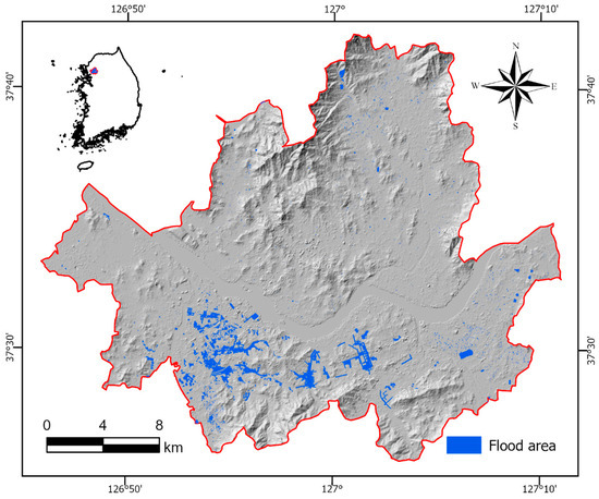
Figure 1.
An overview of the study area showing the selected flooded points recorded in 2022, derived from the Seoul Metropolitan Government database.
3. Materials and Methods
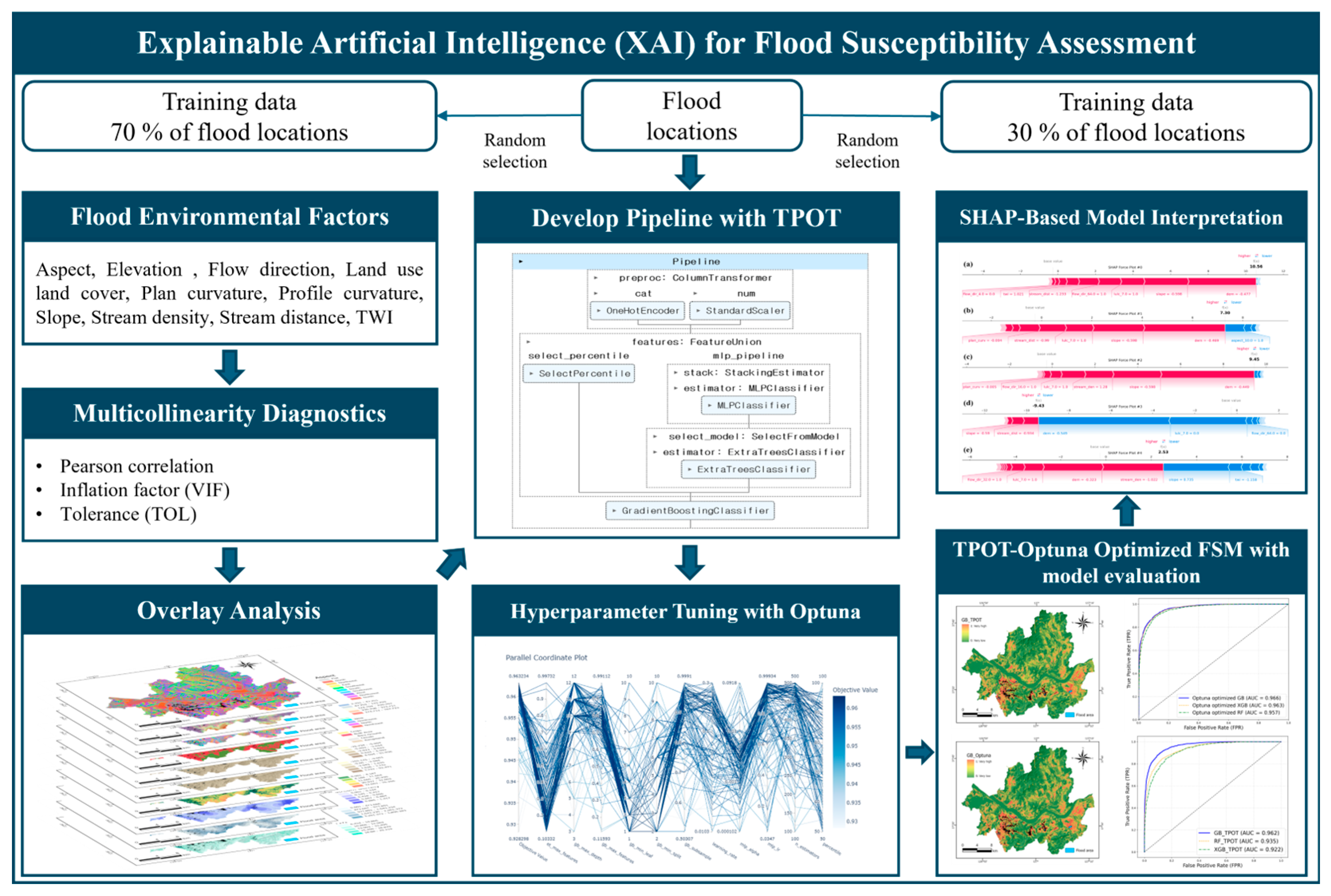
Figure 2 provides a detailed workflow highlighting the sequential procedures conducted to develop a flood susceptibility model. The methodology is structured into six major components. First, spatial datasets relevant to flood-related factors were collected and preprocessed (refer to Section 3.1). Second, multicollinearity and correlation analyses were conducted for factor selection to ensure model robustness (refer to Section 3.2). Third, the TPOT was applied for AutoML model construction and initial pipeline optimization (refer to Section 3.3). Fourth, Optuna, a Bayesian optimization framework, was used to fine-tune hyperparameters of the selected models to improve predictive performance (refer to Section 3.4). Fifth, SHAP was employed to interpret both global and local model outputs, enhancing transparency and explainability (refer to Section 3.5). Finally, the performance of each model was evaluated using established metrics, including AUC, to identify the most accurate flood susceptibility mapping approach (refer to Section 3.6).

Figure 2.
A flowchart of XAI framework for flood susceptibility mapping with TPOT, Optuna, and SHAP.
3.1. Spatial Datasets
This study constructed a flood inventory map based on the official 2022 flood occurrence data provided by the Seoul Metropolitan Government (https://data.seoul.go.kr/dataList/OA-15636/F/1/datasetView.do, accessed on 7 October 2024). The original polygon-format flood records were converted into point features using geometric centroid extraction to enhance spatial precision and minimize potential computational errors. Among the 8668 recorded flooded polygons, 8660 were randomly sampled and labeled as “1” to indicate flood presence. A 500 m buffer [31] was applied to generate absence data to exclude areas potentially influenced by flooding, and randomly selected non-overlapping points were assigned a label of “0.”
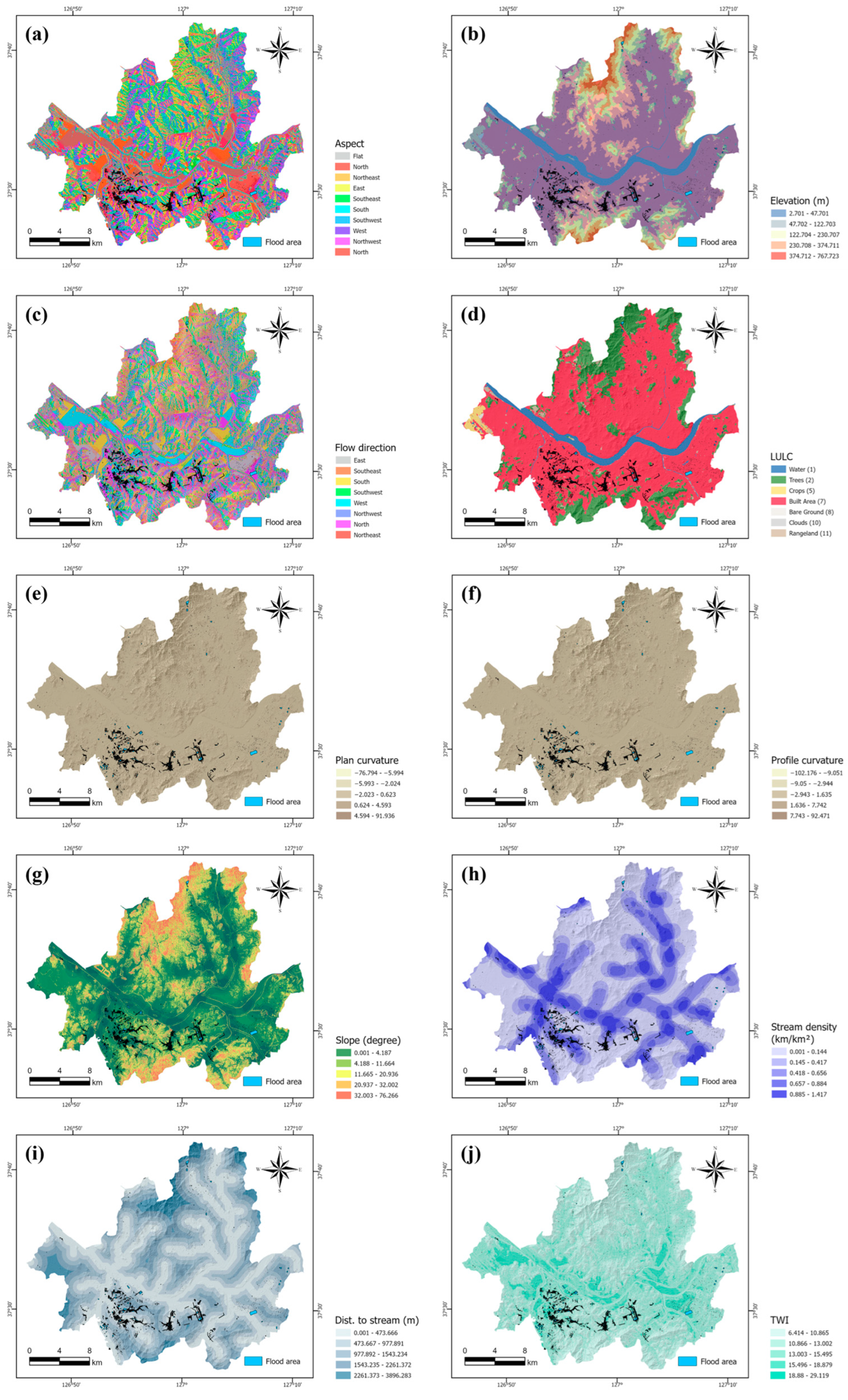
Ten flood-conditioning factors were selected based on previous studies, hydrological relevance, and data availability: elevation (DEM), slope, aspect, profile curvature, plan curvature, flow direction, stream density, distance to stream, topographic wetness index (TWI), and land use and land cover (LULC) [32]. All variables, except for LULC, were derived from a 5 m digital elevation model (DEM) and stream polylines using ArcGIS Pro 3.4. Stream density was computed using the line density function in ArcGIS based on the total length of streams within a 1 km2 neighborhood. LULC data were obtained from the ESRI 10 m Annual Land Cover dataset [33] and resampled to 5 m using nearest-neighbor interpolation to align with other variables. All layers were rasterized to a common spatial resolution and extent, and sampling was performed at flood and non-flood locations to construct the feature matrix for model training. Table 1 summarizes the data sources and formats, while Figure 3 presents their spatial distributions. These harmonized datasets served as inputs for TPOT-based AutoML and Optuna-optimized modeling of flood susceptibility.

Table 1.
The data sources for each flood-conditioning factor used in this study.
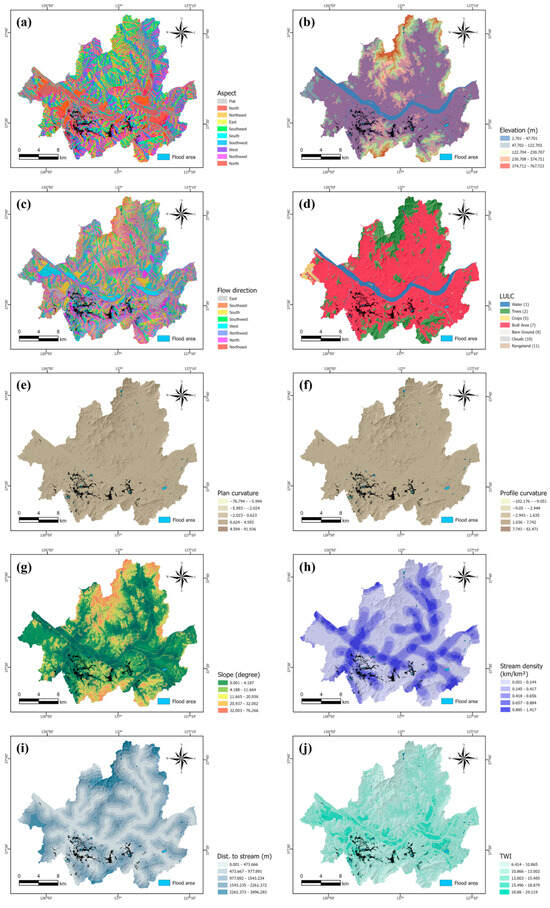
Figure 3.
Thematic maps illustrating the flood-conditioning factors in the Seoul Metropolitan Area considered in this research: (a) aspect, (b) elevation, (c) flow direction, (d) land use and land cover (LULC), (e) plan curvature, (f) profile curvature, (g) slope, (h) stream density, (i) distance to stream, (j) topographic wetness index (TWI).
3.2. Factor Selection
To ensure that the input variables used in AutoML were statistically appropriate and did not introduce multicollinearity, a systematic factor selection process was conducted. Initially, Pearson’s correlation analysis [34] was performed to identify any highly correlated pairs. Variables with a pairwise correlation coefficient |r| ≥ 0.8 were flagged for further investigation, as high collinearity can distort variable importance estimates and reduce model interpretability. Following the correlation analysis, multicollinearity diagnostics were further evaluated using two widely accepted metrics: the Tolerance (TOL) and the Variance Inflation Factor (VIF) [35,36]. TOL measures the proportion of variance in a predictor that is not explained by other predictors, while VIF quantifies how much the variance in a regression coefficient is inflated due to multicollinearity. In this study, variables with TOL values below 0.1 or VIF values exceeding 10 were considered indicative of multicollinearity and were reviewed for potential removal or consolidation. This multi-step screening process ensured that the selected flood-conditioning factors were not only hydrologically relevant but also statistically independent, thereby improving the stability and interpretability of the predictive models. The retained variables were subsequently used as input features in both the TPOT and Optuna model training pipelines for flood susceptibility mapping.
3.3. TPOT for Automated Model Pipeline Optimization
TPOT is an AutoML framework based on genetic algorithm that automates the design and optimization of ML pipelines [37]. It explores a broad search space of pipeline configurations by simulating evolutionary operations [38] such as mutation, crossover, and selection. Each pipeline is treated as an individual, composed of sequential steps including data preprocessing, feature selection, and classification. The optimization process begins with a randomly initialized population of pipelines, which are evaluated using a cross-validation scheme and a user-defined performance metric, typically the area under the ROC curve (ROC-AUC), for classification tasks. Top-performing pipelines are selected as parents, and new offspring are generated through genetic variation. This iterative process continues over multiple generations until the optimization reaches convergence or a predefined stopping criterion is met. TPOT allows for the customization of its search space via configuration dictionaries, enabling researchers to focus the search on specific model types or preprocessing strategies. Its support for parallel processing also makes it efficient for handling high-dimensional geospatial data. In this study, TPOT was applied to identify optimal model architectures for flood susceptibility mapping using geospatial predictors.
3.4. Optuna for Hyperparameter Tuning
Optuna is an open-source hyperparameter optimization framework that employs Bayesian optimization based on the Tree-structured Parzen Estimator (TPE) [39]. This method offers greater search efficiency compared to traditional grid or random search by prioritizing the exploration of promising hyperparameter combinations for constructing high-performing models. The hyperparameter search space is defined using commands such as suggest_float, suggest_int, and suggest_categorical, and each trial is evaluated based on a user-defined objective function. To improve computational efficiency and accelerate convergence, underperforming trials are terminated early through a pruning mechanism [40,41]. Optuna is highly compatible with various ML frameworks (e.g., Scikit-learn, XGBoost) and provides built-in diagnostic tools for visualizing optimization history, hyperparameter importance, and parameter distributions, thereby enhancing interpretability of the tuning process.
In this study, Optuna was employed to optimize hyperparameters within fixed pipeline structures for Gradient Boosting, Random Forest, and XGBoost classifiers. Model performance was assessed using five-fold cross-validation. The best-performing model was further interpreted using SHAP to analyze feature contributions in a spatial context. Unlike TPOT, which automates both pipeline structure and hyperparameter tuning using evolutionary algorithms, Optuna assumes a fixed pipeline architecture and focuses solely on hyperparameter optimization through Bayesian search. The tuning parameters included n_estimators, learning_rate, max_depth, and subsample for Gradient Boosting models.
3.5. SHAP for Model Explainability
To enhance model transparency and interpretability, this study employs SHAP, a game-theoretic approach to explain the output of ML models [42]. SHAP assigns each feature an importance value for a particular prediction by computing Shapley values, which represent the marginal contribution of a feature averaged across all possible combinations of input variables [43]. This unified framework ensures both consistency and local accuracy in explaining model outputs, making it well suited for interpreting complex, nonlinear models such as Gradient Boosting and Random Forest [44].
In this study, SHAP was applied post hoc to the best-performing models optimized through both the TPOT and Optuna frameworks. Global SHAP values were utilized to evaluate the relative contribution of each environmental and topographic factor, enabling the identification of dominant flood-driving variables. Local SHAP explanations were further explored using a force plot to examine how specific feature combinations influenced individual predictions in diverse geospatial contexts. Moreover, SHAP dependence plots were employed to investigate nonlinear feature effects and second-order interactions by visualizing SHAP values against raw feature values, with color encoding used to represent an interacting feature. These combined visualizations, summary plot, dependence plot, and force plot, help validate model behavior and support spatial interpretation of flood susceptibility drivers. By integrating SHAP into the model interpretation pipeline, this study bridges the gap between predictive performance and explainability, thereby improving the transparency, reproducibility, and practical applicability of flood susceptibility mapping [42,43,44].
3.6. Model Evaluation Criteria
To assess model performance comprehensively, this study employed a combination of threshold-independent and threshold-dependent classification metrics. The Area Under the Receiver Operating Characteristic Curve (ROC-AUC) was adopted as the primary metric, as it offers a robust, threshold-independent evaluation of the model’s ability to discriminate between flood and non-flood classes [45]. In addition to ROC-AUC, several threshold-dependent metrics were computed to further evaluate classification performance. Accuracy measures the proportion of correctly classified observations, while Precision represents the proportion of correctly predicted flood events among all instances predicted as floods. Recall (Sensitivity) quantifies the proportion of actual flood events correctly identified by the model. To balance these two aspects, the F1-Score, the harmonic mean of Precision and Recall, was also calculated [46]. Furthermore, the Matthews Correlation Coefficient (MCC) was employed to provide a balanced evaluation, particularly suitable for imbalanced datasets. MCC considers all four categories of the confusion matrix—true positives, false positives, true negatives, and false negatives—making it a reliable indicator of overall model quality [47]. Together, these six evaluation criteria, ROC-AUC, Accuracy, Precision, Recall, F1-Score, and MCC, form a comprehensive framework for assessing both the discriminative capacity and classification reliability of the ML models developed in this study.
4. Results
4.1. Correlation and Multi-Collinearity Analysis
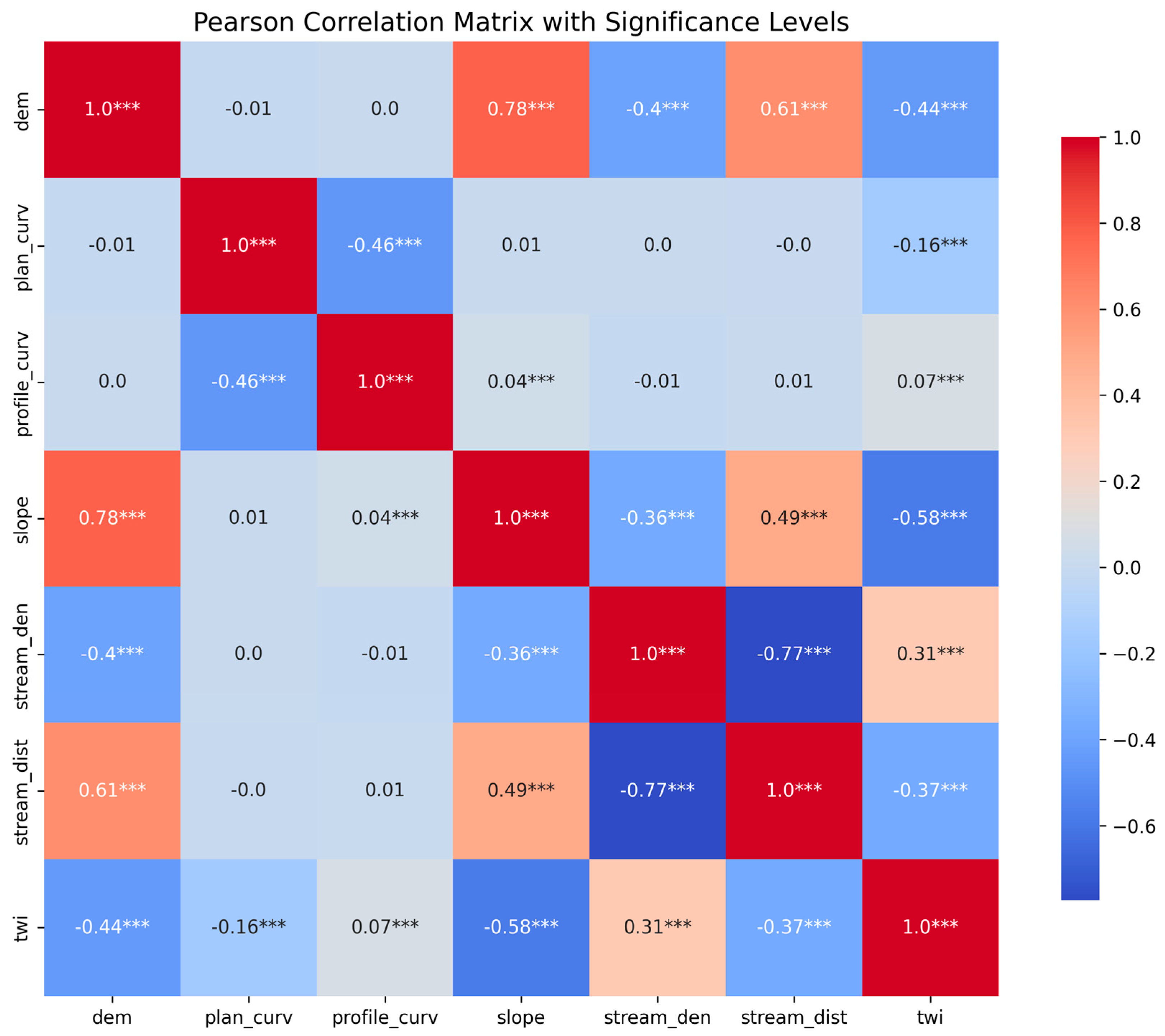
Statistical robustness and minimal redundancy among explanatory variables were ensured through a combination of Inflation Factor (VIF) and Tolerance (TOL) and multicollinearity diagnostics prior to model training. A Pearson correlation matrix was calculated to examine the pairwise linear relationships among the seven continuous flood-conditioning variables. Categorical variables such as LULC, flow direction, and aspect were excluded, as their non-continuous nature violates the assumptions of linear correlation analysis. As illustrated in Figure 4, most variable pairs demonstrated moderate to low correlation coefficients, indicating limited redundancy. Nevertheless, a strong positive correlation (r = 0.775) was observed between elevation (DEM) and slope, while a notable negative correlation (r = −0.773) was found between distance to stream and stream density, implying topographic coupling in hydrological processes. The presence of multicollinearity was further examined using two widely accepted diagnostic metrics: the Variance Inflation Factor (VIF) and Tolerance (TOL). The results summarized in Table 2 show that all variables exhibited VIF values below the critical threshold of 10 and TOL values exceeding the acceptable minimum of 0.1. The highest VIF was recorded for distance to stream (3.406), followed by elevation (3.321) and slope (3.255), all remaining within acceptable limits. These findings confirm the absence of problematic multicollinearity, eliminating the need for variable exclusion. Accordingly, the complete set of ten flood-conditioning factors, including both continuous and categorical variables, was retained for model development using the TPOT and Optuna frameworks. This approach ensures that key hydrological and geomorphological characteristics are comprehensively represented in the flood susceptibility modeling process.

Figure 4.
Pearson’s correlation matrix of continuous flood-conditioning factors. Asterisks indicate statistical significance (*** p < 0.001).
Table 2.
Variance Inflation Factor (VIF) and Tolerance (TOL) values for all predictive variables used in the flood susceptibility model.
4.2. TPOT-Based Flood Susceptibility Mapping
The TPOT framework was employed to automatically optimize ML pipelines for flood susceptibility mapping in Seoul. The final pipeline, selected based on the highest cross-validated ROC-AUC score, integrated three key stages: preprocessing, feature engineering, and classification.
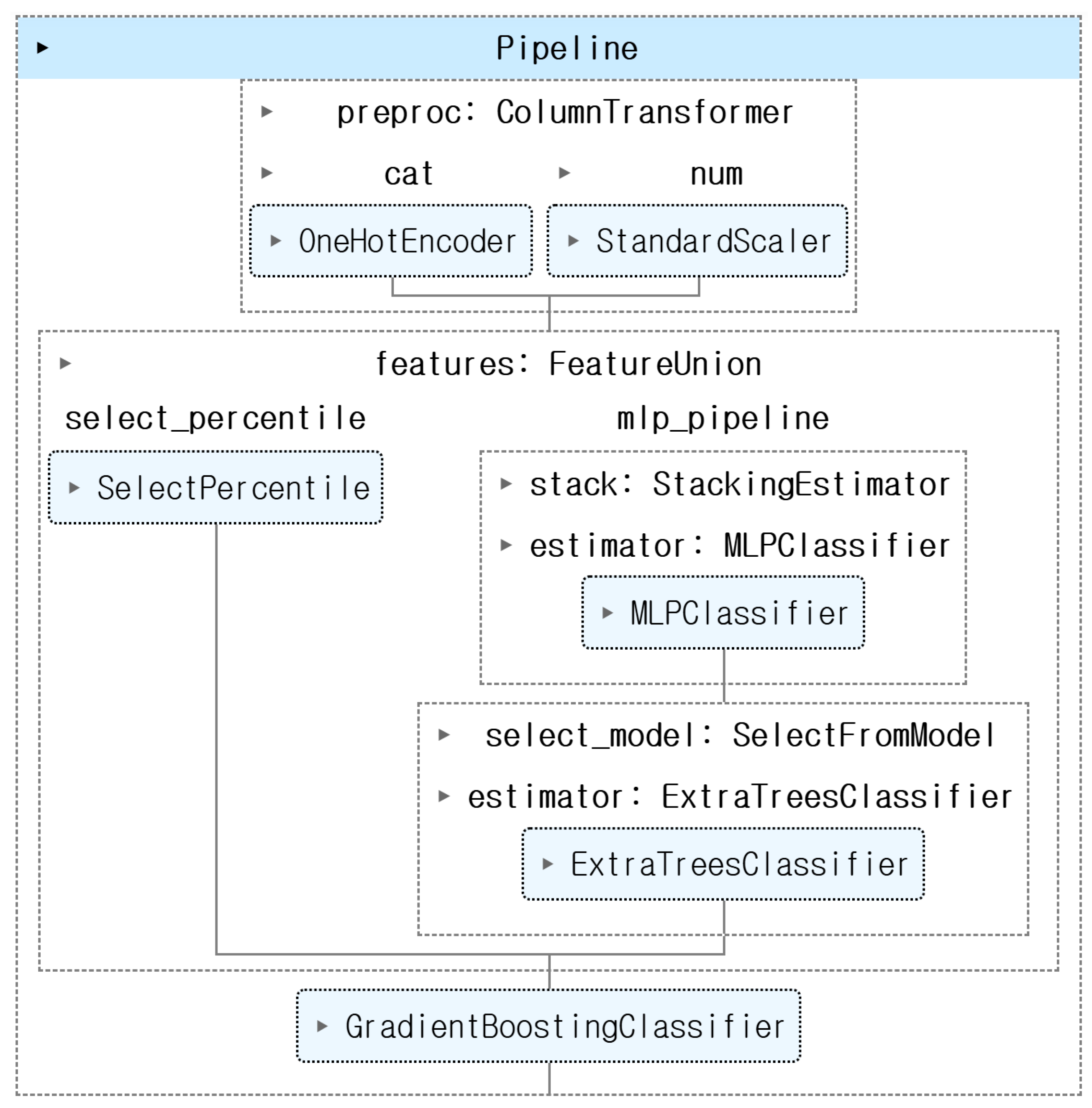
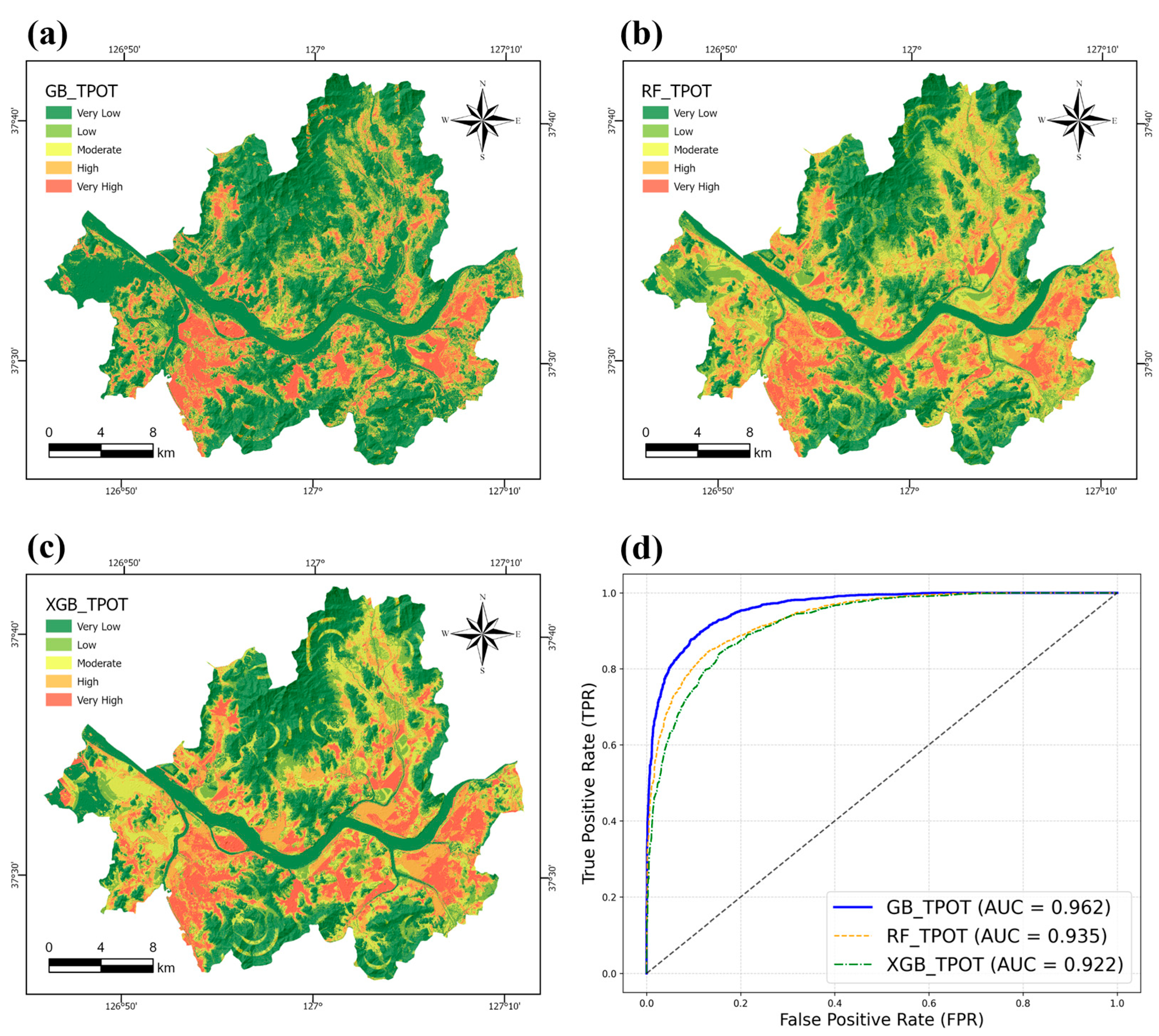
As illustrated in Figure 5, the preprocessing stage utilized a ColumnTransformer that applied one-hot encoding to categorical variables (aspect, flow direction, and LULC) and standardized continuous variables through z-score normalization. In the feature engineering phase, a FeatureUnion was constructed by combining two parallel transformation paths. The first path involved univariate feature selection using SelectPercentile, which retained 78% of the most statistically significant predictors. This selection was based on ANOVA F-values, enabling the pipeline to prioritize features with strong discriminative power across flood and non-flood classes. The second path consisted of a stacking-based sub-pipeline, where an MLPClassifier was used as a meta-estimator to transform the input features, followed by SelectFromModel to extract informative features based on an ExtraTreesClassifier. This combination enabled the pipeline to capture both linear relationships (via SelectPercentile) and complex nonlinear interactions (via stacked MLP and tree-based feature selection). This model achieved the highest predictive performance among all TPOT-generated candidates. The spatial distribution of flood susceptibility across Seoul, predicted by the TPOT-derived models, is visualized in Figure 6a–c. Gradient Boosting yielded the most accurate susceptibility map, followed by Random Forest and XGBoost. Notably, the TPOT-GB model demonstrated strong generalizability even across topographically diverse subregions such as Gangnam and Dobong, underscoring its adaptability to local terrain conditions. Corresponding ROC curves in Figure 6d further support this performance ranking, with the Gradient Boosting model attaining an AUC of 0.962, outperforming RF (0.935) and XGB (0.922). These results highlight TPOT’s ability to construct robust and competitive models without manual intervention.
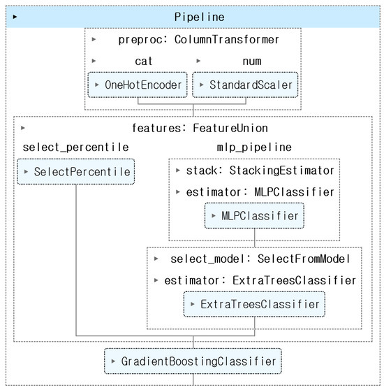
Figure 5.
TPOT framework for automatic optimization of ML pipelines in flood susceptibility mapping. The pipeline includes preprocessing (categorical and numerical encoding), multiple feature selection strategies (SelectPercentile and SelectFromModel), a stacked MLP model, and the final Gradient Boosting classifier. Brief annotations indicate the role of each component to support readers unfamiliar with AutoML workflows.
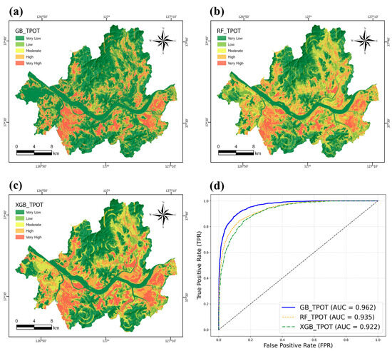
Figure 6.
Flood susceptibility maps produced using each ML model: (a) GB_TPOT, (b) RF _TPOT, (c) XGB_TPOT, and (d) the Receiver Operating Characteristic (ROC) curve and the area under the ROC curve (AUC) for each ML model.
4.3. TPOT-Optuna Enhanced Flood Susceptibility Mapping
To further refine the predictive performance of flood susceptibility models, hyperparameter tuning was conducted using the Optuna framework based on the top three ensemble classifiers identified through TPOT: Gradient Boosting (GB), Random Forest (RF), and XGBoost (XGB). Rather than relying on TPOT’s internal optimization, Optuna was applied to these models independently to explore more fine-grained hyperparameter spaces within a fixed pipeline structure. This two-stage approach leverages the structural automation of TPOT for pipeline discovery and the precision of Optuna’s Bayesian optimization for targeted parameter tuning.
As shown in Figure 7a–c, the flood susceptibility maps generated by the Optuna-optimized models reveal spatial patterns of flood-prone areas across Seoul. Among the three models, the GB classifier yielded the most concentrated and spatially coherent distribution of high-susceptibility zones, particularly along low-lying riverine corridors and densely urbanized regions. The XGB and RF models showed similar spatial patterns but with slightly more dispersed high-risk zones. The slightly more scattered pattern in XGB may reflect its sensitivity to noisy geospatial inputs or overfitting tendencies in high-dimensional feature spaces. Visual comparison with historical flood records (blue polygons) indicates that all three models successfully captured many of the observed inundation areas, demonstrating spatial consistency with empirical data. However, future work may further quantify this agreement using spatial overlap metrics such as Intersection over Union (IoU) or pixel-wise accuracy, enhancing the spatial validation framework. Model performance was quantitatively assessed using ROC-AUC scores on the test dataset. As illustrated in Figure 7d, the Optuna-tuned GB model achieved the highest AUC of 0.966, followed closely by XGB (0.963) and RF (0.957). These values represent measurable improvements over TPOT-only configurations. For instance, the Optuna-optimized GB model achieved optimal values of learning_rate = 0.12, max_depth = 10, and n_estimators = 430, highlighting the importance of fine-tuning even in strong baseline models. Unlike TPOT’s stochastic search process, Optuna’s pruning mechanism and reproducible trials enabled controlled convergence toward globally optimal hyperparameters.
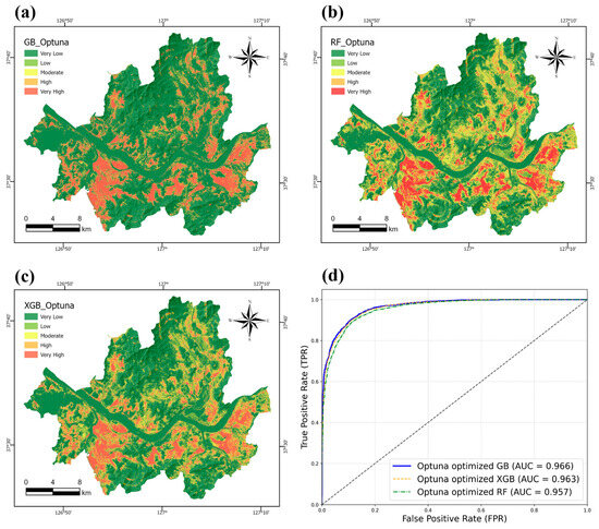
Figure 7.
Flood susceptibility maps produced using each ML model: (a) GB_Optuna, (b) RF _ Optuna, (c) XGB_ Optuna, and (d) the Receiver Operating Characteristic (ROC) curve and the area under the ROC curve (AUC) for each ML model.
The Optuna-enhanced modeling strategy not only improved prediction accuracy but also facilitated greater transparency in the optimization process. The combination of TPOT’s pipeline search and Optuna’s controlled tuning framework demonstrates the value of hybrid AutoML strategies in geospatial hazard modeling. These improvements hold practical implications for urban flood preparedness, offering decision-makers accurate and explainable spatial risk assessments. This integrated approach enables researchers to balance exploratory flexibility with reproducibility and interpretability, which is particularly important in operational flood risk assessment contexts. As shown in Figure 8, the predicted flood susceptibility varies by model and optimization strategy. GB_Optuna emphasizes low-risk areas, while RF_TPOT and XGB_TPOT highlight more moderate- to-high-risk zones, indicating different spatial sensitivities across classifiers.
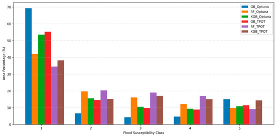
Figure 8.
Comparison of area percentage by flood susceptibility class predicted by six models: Gradient Boosting (GB), Random Forest (RF), and XGBoost (XGB), each optimized using TPOT and Optuna.
4.4. Model Performance
To evaluate the classification capabilities of the developed models, six performance metrics were computed: the Area Under the Receiver Operating Characteristic Curve (ROC AUC), Accuracy, Precision, Recall, F1-Score, and Matthews Correlation Coefficient (MCC). Table 3 presents a side-by-side comparison of all models using bar charts for each metric. These metrics provide a comprehensive assessment of both the discriminative power and the classification robustness—especially important for imbalanced environmental data. Among the TPOT-generated models, the best-performing pipeline was the Gradient Boosting classifier (TPOT_GB), which achieved an AUC of 0.962, an Accuracy of 0.894, an F1-Score of 0.895, and an MCC of 0.787. The Random Forest model (TPOT_RF) followed with an AUC of 0.935 and slightly lower values for all other metrics. The XGBoost variant (TPOT_XGB) recorded the lowest performance among the three, with an AUC of 0.922 and MCC of 0.703. These results suggest that TPOT’s automated pipeline optimization effectively identified a high-performing baseline configuration, particularly with Gradient Boosting. In contrast, the Optuna-optimized models showed consistent improvement across all six metrics, highlighting the benefit of Bayesian hyperparameter tuning. The Optuna_GB model reached the highest AUC (0.966), followed by Optuna_XGB (0.963) and Optuna_RF (0.957). Notably, Optuna_GB improved MCC by 0.009 compared to TPOT_GB (from 0.787 to 0.796), which reflects better predictive balance and reduced bias between classes. The Accuracy and F1-Score also slightly increased, confirming gains in both Precision and Recall. Figure 8 illustrates a side-by-side comparison of all models using bar charts for each metric. As visualized, the Optuna-tuned models consistently outperform their TPOT counterparts across the board. In particular, Gradient Boosting showed the most stable and superior performance in ROC AUC, F1-Score, and MCC—demonstrating both high discrimination and classification reliability. These findings underscore the strength of the two-stage AutoML approach, where TPOT provides structural discovery and Optuna delivers fine-grained parameter refinement. The integration of these two frameworks results in a balanced trade-off between automation, control, and model generalization, which is essential for operational flood susceptibility assessment.
Table 3.
Performance metrics of ensemble classifiers optimized using TPOT and Optuna.
As visualized, the Optuna-tuned models consistently outperform their TPOT counterparts across the board. In particular, Gradient Boosting showed the most stable and superior performance in ROC AUC, F1-Score, and MCC, demonstrating both high discrimination and classification reliability. These findings underscore the strength of the two-stage AutoML approach, where TPOT provides structural discovery and Optuna delivers fine-grained parameter refinement. The integration of these two frameworks results in a balanced trade-off between automation, control, and model generalization, which is essential for operational flood susceptibility assessment. The limited performance improvement of the GB model after Optuna tuning can be attributed to the fact that the TPOT-derived GB pipeline was already close to optimal in terms of hyperparameter configuration. Consequently, the additional tuning space explored by Optuna led to only marginal gains. In contrast, the initial configurations of the RF and XGB models were more flexible, allowing Optuna to achieve more substantial performance enhancements. While RF often demonstrates strong predictive performance in other studies, its relatively lower performance in this study may be explained by the spatial heterogeneity and class imbalance present in the flood susceptibility data. Tree-based ensembles such as RF generally perform well on balanced datasets, whereas GB tends to be more robust in handling skewed or noisy data through its sequential learning mechanism. Moreover, the modeling approach adopted in this study prioritized both predictive accuracy and interpretability, and GB offered the most favorable balance between these two aspects.
4.5. SHAP-Based Model Interpretation
To enhance the interpretability of the Gradient Boosting model used for flood susceptibility mapping, SHAP was applied to quantify both global and local contributions of each feature. This section presents SHAP outputs through four visualization types: summary plot, dependence plot, and force plot.
4.5.1. Summary Plot
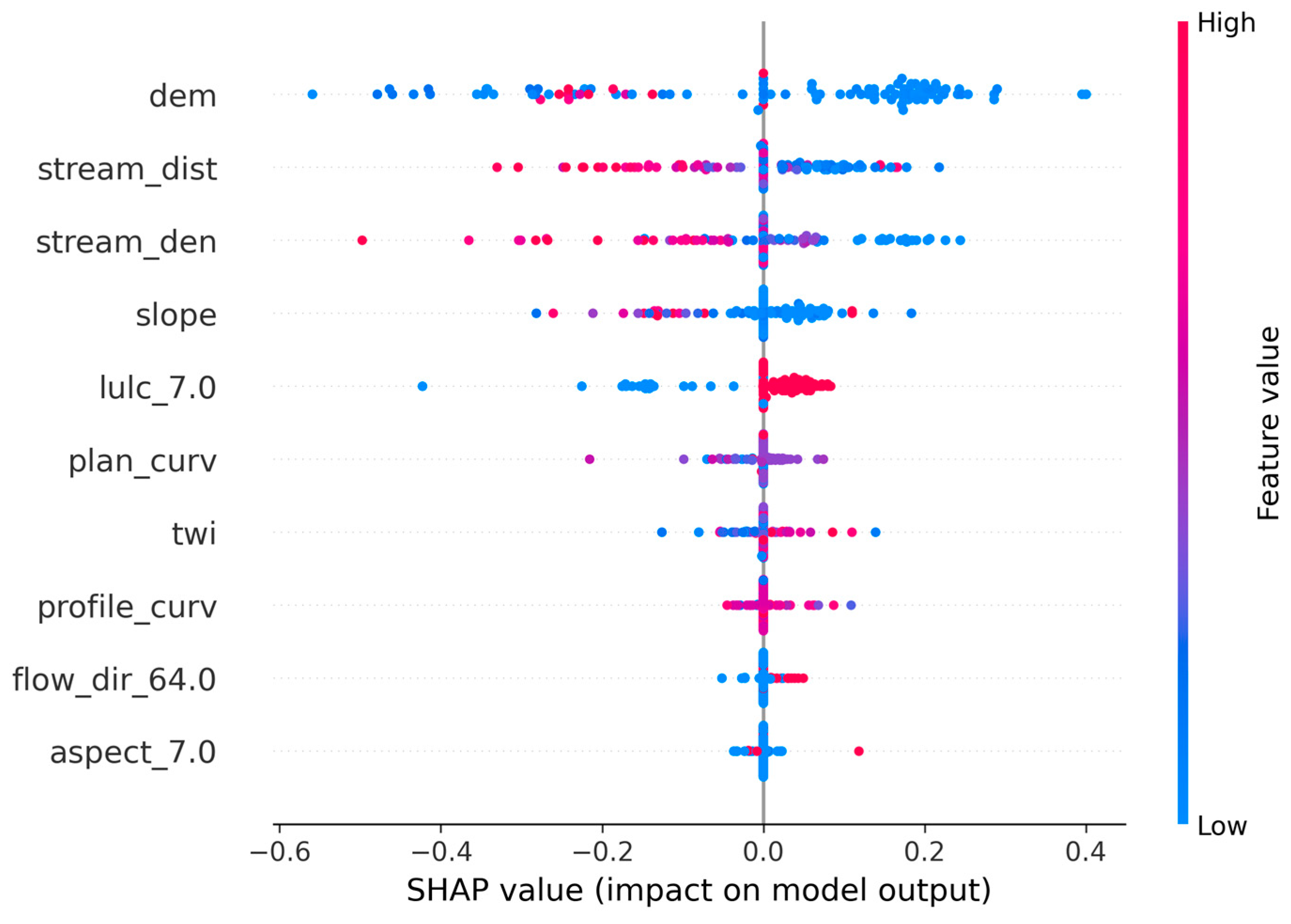
The SHAP summary plot (Figure 9) provides a global view of the relative importance and directional impact of the top ten features.
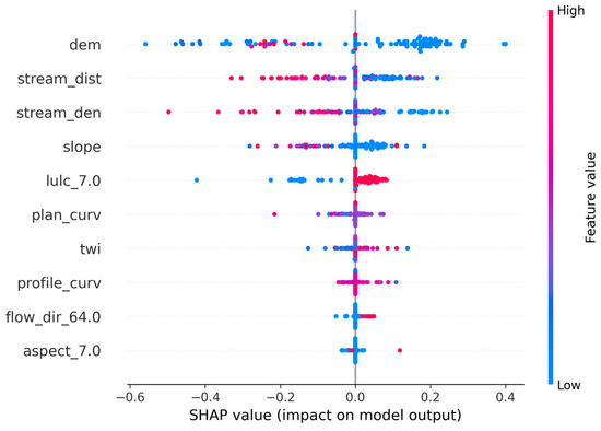
Figure 9.
SHAP summary plot illustrating the contribution of each conditioning factor to model predictions. Feature values are color-coded (red = high, blue = low), and SHAP values were computed using the TreeSHAP algorithm. dem, stream distance, and stream density exhibit the highest influence on the model output.
Notably, ‘dem’, ‘stream_dist’, ‘stream_den’, ‘slope’, and ‘lulc_7.0’ emerged as the most influential predictors. Lower elevation (‘dem’), shorter distance to streams (‘stream_dist’), and higher stream density (‘stream_den’) were associated with positive SHAP values, indicating increased flood susceptibility. The land use class ‘lulc_7.0’, corresponding to built-up areas, also contributed positively, reflecting the role of impervious surfaces in amplifying surface runoff. Furthermore, the color gradient in Figure 9 demonstrates how feature values affect model output: blue indicates low feature values, and red indicates high feature values. For instance, low ‘dem’ and ‘stream_dist’ values (blue) result in high SHAP contributions to flood risk, aligning with hydrological understanding of flood-prone lowlands.
Features such as dem, stream_dist, stream_den, slope, and lulc_7.0 were found to have the greatest influence on model predictions. Specifically, low elevation (dem), short distance to stream (stream_dist), and high stream density (stream_den) positively contributed to higher flood risk predictions. The land use category lulc_7.0, corresponding to impervious surfaces or urbanized areas, also had a strong positive effect.
4.5.2. Dependence Plot
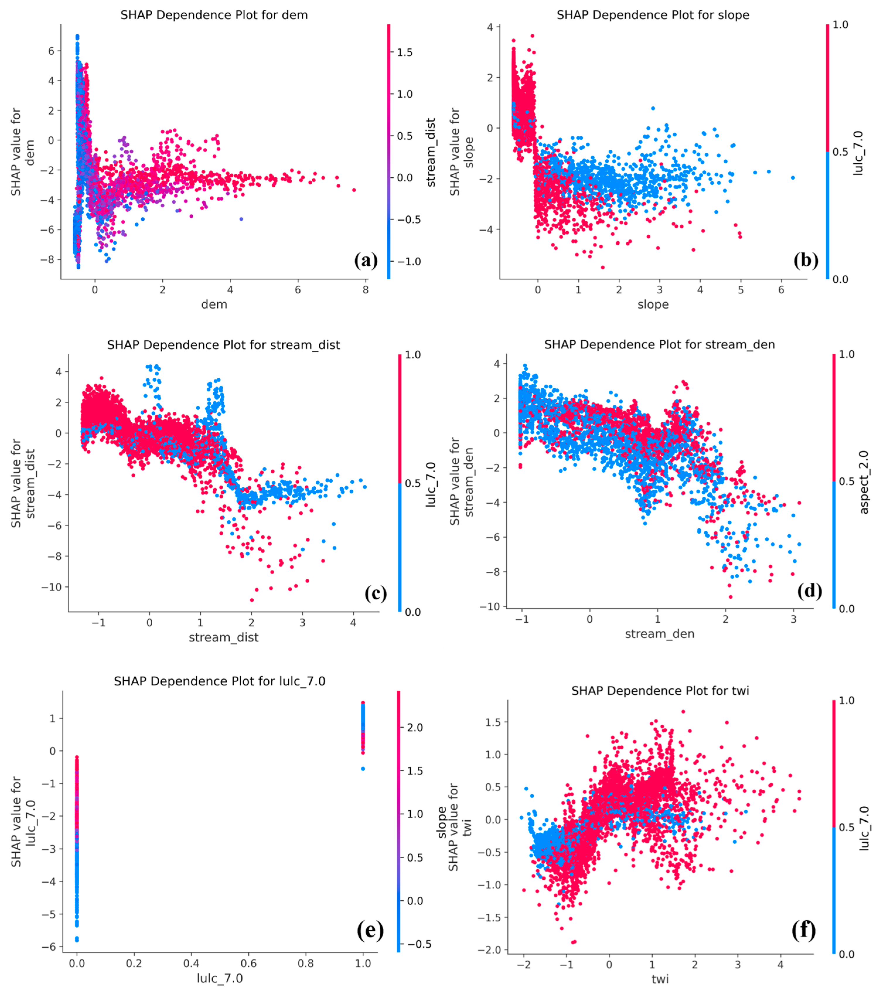
SHAP dependence plots visualize how the model’s predicted flood susceptibility is influenced by the actual values of each feature while also highlighting feature interactions through color gradients (Figure 10).
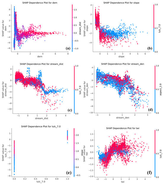
Figure 10.
SHAP dependence plots showing the relationship between input feature values (x-axis) and their corresponding SHAP values (y-axis) for major flood-conditioning factors: (a) elevation (DEM), (b) slope, (c) stream distance, (d) stream density, (e) built-up area (LULC_7.0), and (f) topographic wetness index (TWI). Each point represents a prediction instance, with color indicating the value of an interacting feature. The x-axis represents the original value of the input feature, while the y-axis indicates the SHAP value, which quantifies the feature’s impact on the model output. Higher absolute SHAP values correspond to stronger influence, positive or negative, on the predicted flood susceptibility.
These plots reveal that flood risk is not governed by individual variables alone, but emerges from complex interactions between terrain, hydrology, and land use. Figure 10a shows that lower elevation (dem) values correspond to higher SHAP values, confirming that low-lying areas are more flood-prone. In Figure 10b, slope is inversely related to SHAP values, indicating that flatter terrain increases flood risk. Figure 10c displays a nonlinear decline in SHAP value with increasing distance from streams, highlighting the vulnerability of near-stream areas. In Figure 10d, stream density contributes positively to flood susceptibility, with north-facing slopes (aspect_2.0) enhancing this effect. Figure 10e presents a SHAP dependence plot for the binary variable lulc_7.0, which indicates whether a given pixel is classified as built-up area (LULC class 7). The x-axis represents the value of the binary indicator (0 for non-built-up areas and 1 for built-up areas), while the y-axis shows the corresponding SHAP value, quantifying its contribution to the model’s flood susceptibility prediction. The color gradient reflects slope values, where red represents low slope and blue indicates steep terrain. The plot reveals that built-up areas (lulc_7.0 = 1) consistently contribute to an increased flood risk, especially in areas with gentle slopes. In contrast, non-built-up areas (lulc_7.0 = 0) have minimal influence on the prediction, as reflected by SHAP values near zero. Lastly, Figure 10f shows that higher TWI values are associated with greater flood susceptibility. This pattern is amplified in urban environments, where water accumulation and impervious surfaces interact to elevate flood risk. Overall, the SHAP dependence plots demonstrate that accurate flood prediction requires accounting for both direct feature effects and cross-variable interactions. The SHAP dependence plots indicate that flood risk increases notably in areas where low elevation (DEM), low slope, short distance to streams, and high stream density coincide with developed land (LULC_7.0 = 1). These interacting factors collectively amplify susceptibility, suggesting that urbanized low-lying zones near dense stream networks are the most flood-prone areas in the study region. The SHAP dependence plots reveal that low elevation, low slope, short distance to streams, and high stream density jointly amplify flood susceptibility, particularly when combined with built-up land cover. These factors interact synergistically in flat, urbanized lowland areas, where water tends to accumulate and drainage is limited. Based on the interaction of these variables, the most flood-susceptible areas are low-lying, densely built-up regions located near concentrated stream networks.
4.5.3. Force Plot
To further enhance local model interpretability, SHAP force plots were generated to explain how specific combinations of feature values contribute to individual prediction outcomes (Figure 11).
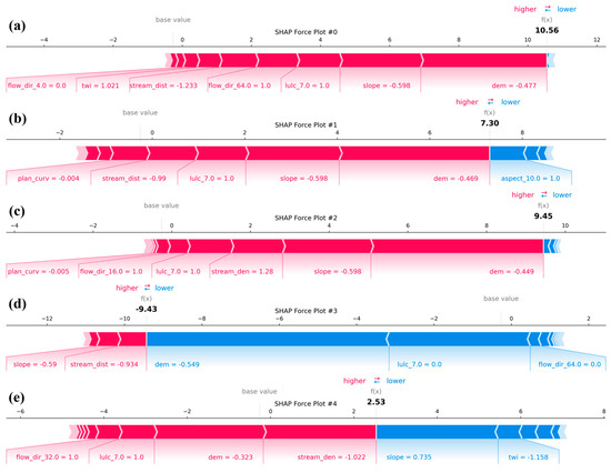
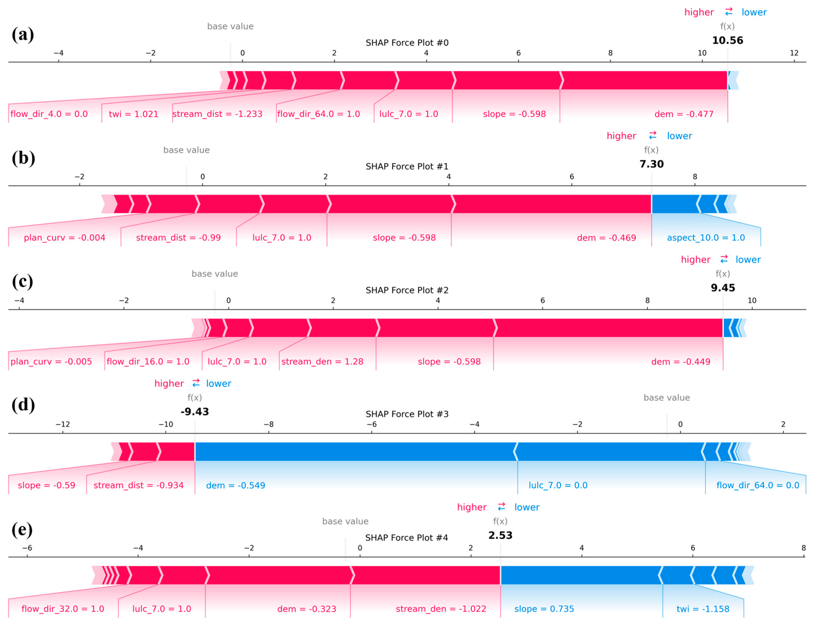
Figure 11.
SHAP force plots illustrating the contribution of individual features to flood susceptibility prediction for selected instances. The x-axis shows SHAP values relative to the model’s base value (mean prediction), with red indicating features that increase the prediction and blue indicating those that decrease it. (a) High susceptibility (10.56), mainly influenced by stream distance and TWI. (b) High susceptibility (7.30), primarily driven by LULC and stream distance. (c) High susceptibility (9.45), attributed to stream density, flow direction, and LULC. (d) Very low susceptibility (−9.43), mainly decreased by elevation (DEM), LULC, and flow direction. (e) Low-to-moderate susceptibility (2.53), with increased risk associated with stream density, flow direction, and LULC.
Each plot illustrates the shift from the model’s base value to the final prediction, with red arrows representing features that push the prediction higher (toward flood risk) and blue arrows indicating features that lower the risk. These instance-level visualizations enable a precise understanding of the internal logic behind the model’s output. Figure 11a shows a very high prediction value of 10.56, strongly influenced by a combination of low elevation (dem), gentle slope, and built-up area (lulc_7.0 = 1). These features align with known flood-prone conditions in urban lowlands. Figure 11b presents a slightly lower prediction of 7.30, where aspect_10.0 (North-facing slope) exerts a notable negative effect, partially offsetting the positive contributions from lulc_7.0 and low slope. Figure 11c reflects another high-risk case (9.45), where flow direction (flow_dir_16.0), high stream density, and lulc_7.0 jointly amplify the flood susceptibility. Figure 11d illustrates a low-risk prediction of –9.43, driven by high elevation, large stream distance, and steep slope, all of which mitigate flood potential. Figure 11e represents a moderate-risk case (2.53) with mixed feature effects: stream density and lulc_7.0 increase the risk, while twi, dem, and slope decrease it, resulting in a balanced output. These representative force plots confirm that flood susceptibility predictions are not solely influenced by individual features but result from the complex interplay between topographic, hydrologic, and land use variables. Such localized explanations are critical for validating model behavior, especially in policy-relevant applications where transparency and spatial specificity are essential.
4.6. Rationale for Sample-Based SHAP Visualizations
While global interpretability tools such as the SHAP summary plot offer macroscopic insights into feature influence across the dataset, local explanations, through force plots, allow for granular examination of individual predictions (Figure 11). In this study, representative samples (Sample #0 to #4) were carefully selected to capture varying geospatial contexts, including low-lying urban zones, hilly terrain, and stream-adjacent regions. These localized SHAP visualizations serve two primary purposes. First, they enhance local interpretability by tracing how specific combinations of feature values affect the model output relative to the base value. Second, they enable comparative understanding of how flood risk drivers differ spatially across contrasting topographies.
Notably, while SHAP dependence plots are often interpreted as global tools, they are composed of individual predictions, each dot reflecting one instance, allowing for secondary interaction effects to be visualized through color encoding. By limiting the analysis to 5–10 diverse yet representative samples, the interpretability remains tractable without losing fidelity. This targeted approach confirms that flood susceptibility is not only driven by global trends but also by localized conditions, thereby reinforcing the transparency and spatial sensitivity of the optimized model.
5. Discussion
This section critically interprets the results through the lens of previous studies and methodological innovation, offering insights into the advancement of AutoML-driven flood susceptibility mapping. First, our findings were benchmarked against existing flood susceptibility models in Seoul. The TPOT–Optuna models achieved higher AUC scores and more spatially coherent risk zones compared to conventional methods such as Random Forest, Logistic Regression, and DNNs (refer to Section 5.1). These results underscore the limitations of static or manually tuned models in capturing dynamic hydrological patterns. Second, the hybrid AutoML framework, integrating TPOT’s evolutionary search and Optuna’s Bayesian tuning, proved especially effective. While TPOT offered structural flexibility and end-to-end automation, Optuna enabled refined, reproducible hyperparameter tuning within expert-informed pipelines (refer to Section 5.2). This complementary strategy illustrates the value of combining exploratory and focused optimization techniques. Third, model interpretability was addressed through SHAP visualizations and Optuna diagnostics (refer to Section 5.3). SHAP provided global and local explanations, revealing complex feature interactions, while Optuna’s history and importance plots enhanced understanding of the optimization dynamics. This dual-layered approach supports explainable AI (XAI) in environmental modeling, enabling transparent, interpretable, and reproducible decision-making frameworks for flood risk assessment.
5.1. Comparison with Previous Studies
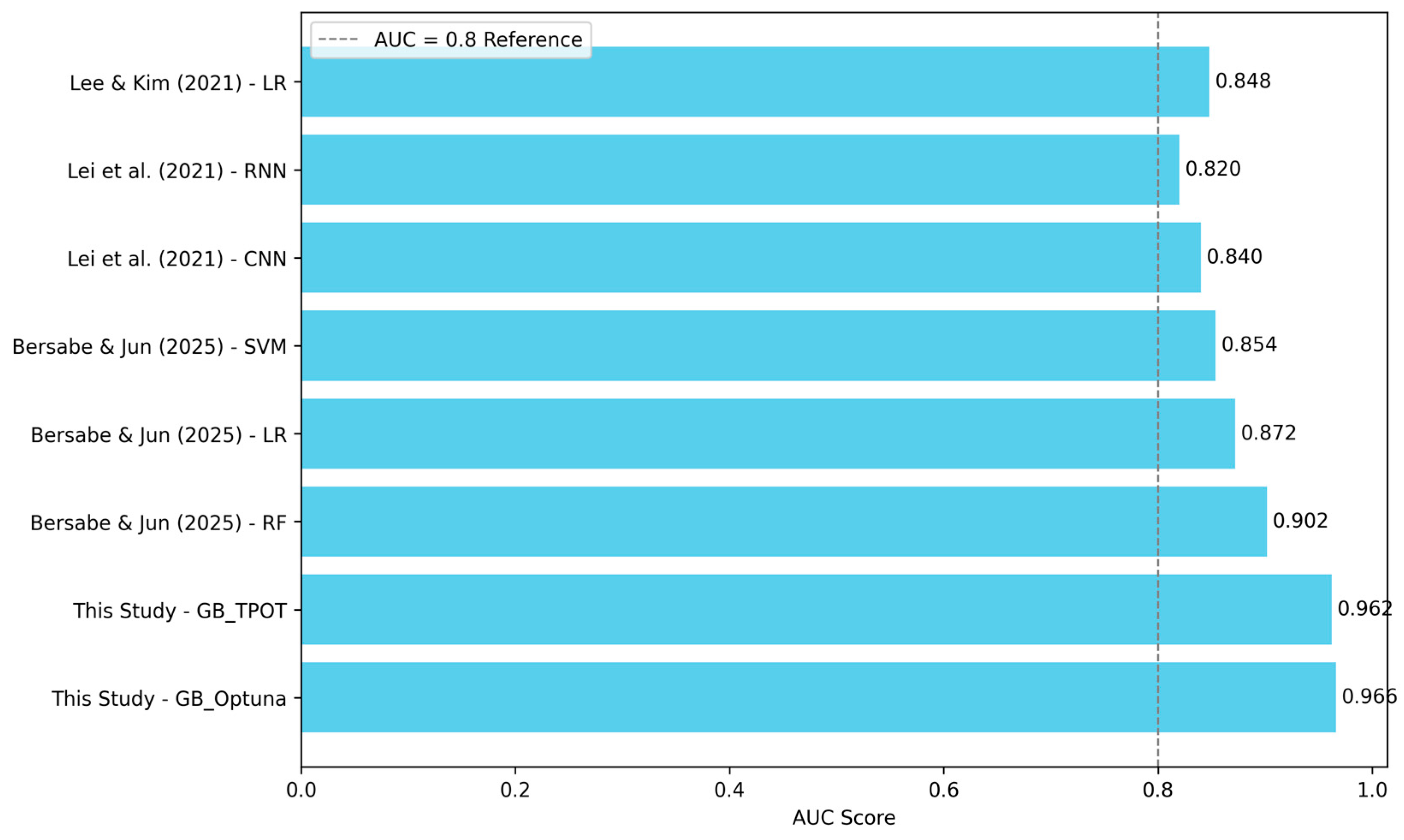
Over the past decade, various ML and statistical approaches have been applied to flood susceptibility mapping in Seoul. Lee and Kim [48] used a logistic regression model incorporating rainfall and topographic data, achieving an AUC of 0.848. While this study highlighted the utility of precipitation data, its reliance on static statistical modeling limited adaptability. Lei et al. [49] employed deep learning frameworks such as CNN (AUC = 0.840) and RNN (AUC = 0.820), offering improved feature representation but lacking interpretability and generalizability due to limited input diversity. More recently, Bersabe and Jun [50] introduced urban infrastructure variables such as sewer density and proximity to storm drains into a Random Forest model, achieving a notable AUC of 0.902. While these results underscore the value of engineered features in urban flood modeling, such variables were not included in the present study due to the lack of spatially detailed and validated infrastructure data across the study area. To ensure consistency and reproducibility, this study focused on publicly available topographic and hydrologic factors. Despite differences in variable selection, both studies consistently identify elevation and stream proximity as dominant predictors. In addition, our findings highlight the critical influence of stream density and built-up areas (LULC), particularly in low-lying and densely developed zones. These patterns reflect the urban flood dynamics of Seoul, where terrain and land use characteristics strongly govern flood susceptibility. This convergence on topographic and hydrologic factors reaffirms their fundamental role in urban flood modeling for the region. In comparison, the current study achieved superior performance using only topographic and land-use variables, without infrastructure-specific inputs. The Optuna-optimized Gradient Boosting model reached an AUC of 0.966, outperforming all previous models (Figure 12). This marks a 6.4% improvement over the highest prior result [50], achieved through advanced AutoML techniques including TPOT-based pipeline search and Bayesian tuning via Optuna.
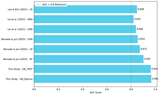
Figure 12.
Comparison of AUC scores from previous flood susceptibility studies in Seoul [48,49,50].
This outcome emphasizes that performance gains can be realized not solely through new data inputs but also by leveraging evolutionary and probabilistic optimization strategies. Furthermore, model explainability, lacking in many earlier studies, was addressed through SHAP visualizations, enhancing transparency and stakeholder confidence. Thus, the proposed approach contributes methodologically and practically to the advancement of explainable, high-accuracy flood susceptibility modeling in urban environments.
5.2. TPOT–Optuna Hybrid Optimization
Building on the pipeline architectures explored in Section 4.2 and the improved results described in Section 4.3, this section further contextualizes the contribution of the TPOT–Optuna hybrid strategy. The integration of TPOT and Optuna in this study offers a hybrid optimization strategy that leverages the strengths of both evolutionary and Bayesian methods. TPOT facilitates the automated construction of ML pipelines through genetic programming, enabling the discovery of novel and high-performing combinations of preprocessing, feature selection, and classification components. This evolutionary exploration is particularly effective for identifying structural configurations that may be overlooked in manual model design, thereby reducing human bias and enhancing automation. However, the stochastic nature of TPOT’s pipeline search often results in variability across runs and can limit reproducibility. Furthermore, TPOT’s reliance on fixed evolutionary parameters, such as mutation and crossover rates, constrains its capacity for fine-grained control over hyperparameter spaces. To address these limitations, Optuna was applied as a secondary optimization framework focused on hyperparameter refinement. By utilizing Bayesian optimization with a Tree-structured Parzen Estimator (TPE), Optuna efficiently explores the search space of selected classifiers and fine-tunes their hyperparameters to achieve optimal performance. The results demonstrate that combining TPOT’s structural exploration with Optuna’s precise tuning significantly enhances model performance. The Optuna-optimized Gradient Boosting model outperformed all TPOT-only pipelines, achieving an AUC of 0.966 compared to 0.962 from TPOT’s best pipeline (see Figure 7d). While the numerical gain in AUC may appear modest, it reflects a significant reduction in misclassification errors in highly imbalanced environmental datasets.
Notably, this improvement was achieved without introducing additional features or model types but rather by refining existing components derived from TPOT. In addition, this two-stage optimization strategy improves both interpretability and reproducibility. By decoupling pipeline architecture generation from hyperparameter tuning, researchers can gain greater transparency into the modeling process while retaining control over model design. This modular workflow is especially beneficial for environmental applications, where domain expertise can inform initial pipeline structures, and automated tuning can maximize predictive accuracy. Overall, the TPOT–Optuna approach presents a flexible and powerful framework for flood susceptibility modeling, balancing the benefits of exploratory automation with targeted optimization. This integration demonstrates potential for broader adoption in geospatial ML tasks that demand both model complexity and transparency.
5.3. Model Explainability via SHAP and Optuna for XAI
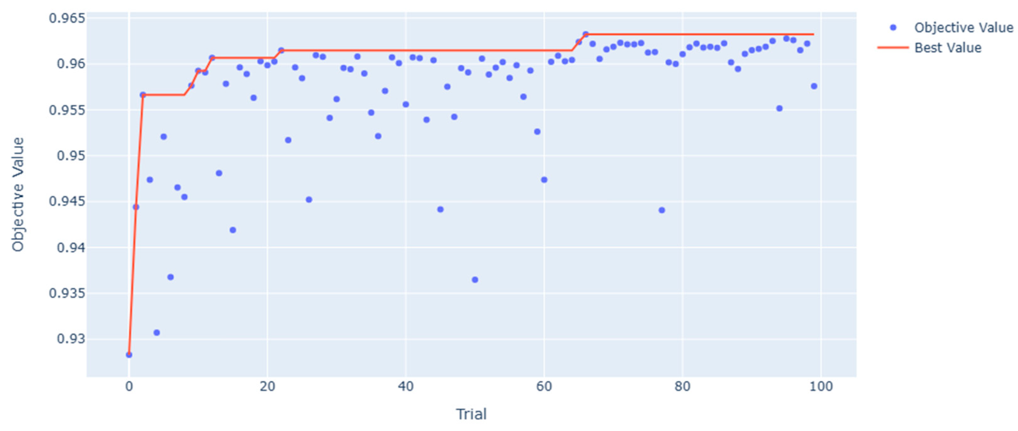
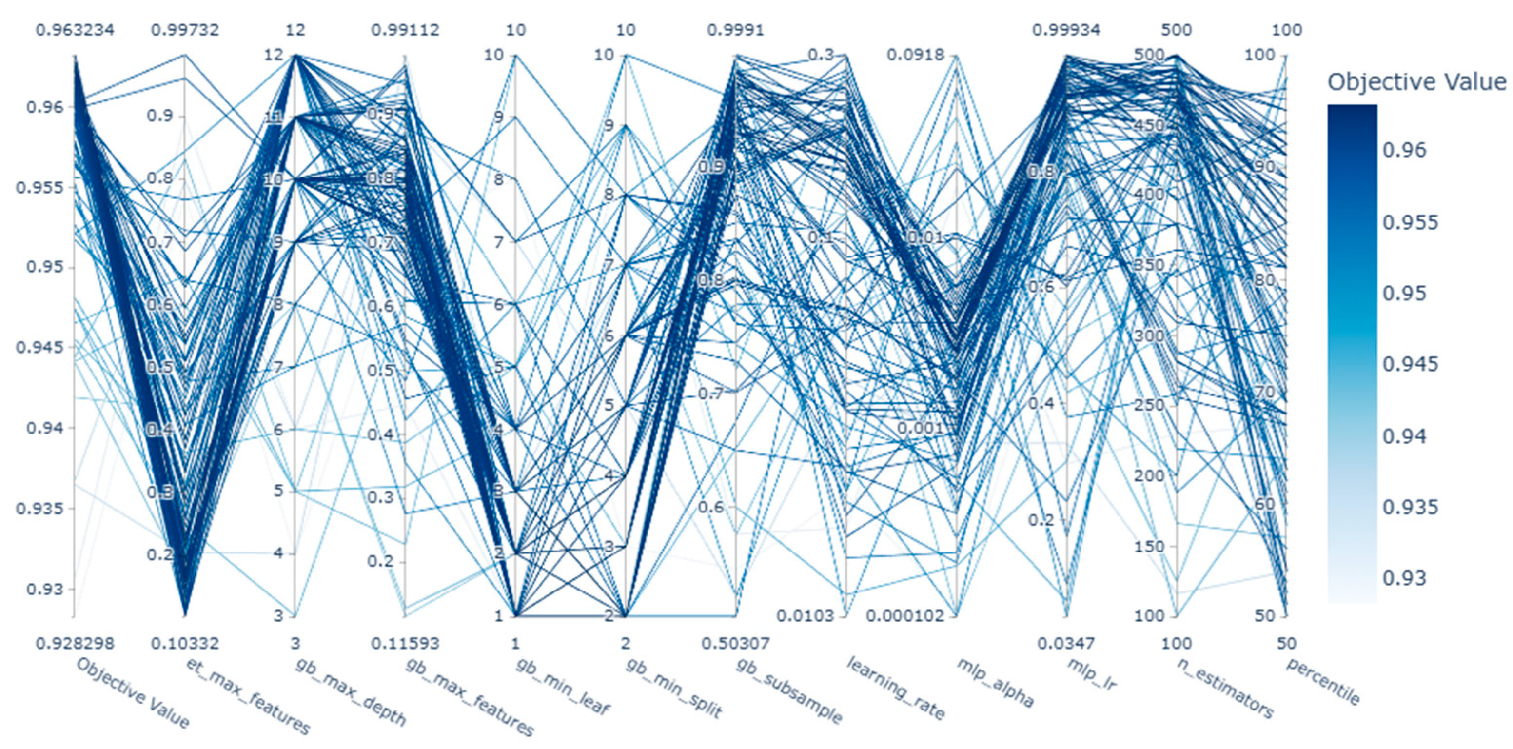
In the context of flood susceptibility modeling, the demand for XAI has grown significantly, especially as predictive models become more complex and opaque. To address this, the current study employed both SHAP and Optuna’s visualization toolkit to enhance interpretability at both the model and hyperparameter levels. SHAP visualizations provided granular insights into how individual features influenced global and local predictions. Through a combination of summary plots, dependence plots, and force plots, the internal logic of the Gradient Boosting model was visualized in a human-interpretable form. These outputs allow practitioners to validate model behavior against hydrological knowledge and support evidence-based decision-making in high-stakes contexts such as urban flood risk management. For example, the SHAP summary plot (Figure 9) highlighted that elevation (dem), distance to stream (stream_dist), and slope were among the most influential variables in determining flood risk. Dependence plots (Figure 10) revealed nonlinear feature behaviors and interactions, such as the increased flood susceptibility in low-slope built-up areas (lulc_7.0 = 1). Force plots (Figure 11) demonstrated how individual features contributed additively to high- or low-risk predictions. These local explanations are particularly valuable for interpreting model predictions at specific sites and validating them against field-based flood reports. In parallel, Optuna’s visualization tools offered transparency into the hyperparameter optimization process, which is often treated as a black-box procedure in ML workflows. The optimization history plot (Figure 13) demonstrated rapid convergence to a high-performing model within 20–30 trials. The parallel coordinate plot (Figure 14) illustrated how different hyperparameter combinations collectively impacted model performance, providing an overview of interaction effects. The hyperparameter importance chart (Figure 15) revealed that gb_max_depth had the most substantial influence on model accuracy, followed by gb_max_features and learning_rate. Finally, scatter plots across the hyperparameter search space (Figure 16) confirmed the relationship between parameter ranges and objective values, offering fine-grained insight into optimal parameter settings. These Optuna-based visualizations serve as an essential complement to SHAP. While SHAP explains what drives model predictions, Optuna clarifies how model configurations influence performance. Together, they fulfill complementary roles in the XAI pipeline: SHAP provides data-driven transparency, and Optuna contributes algorithmic transparency during model development. This synergy not only enhances reproducibility and stakeholder trust but also enables more informed decision-making in geospatial modeling and flood risk analysis.

Figure 13.
Optimization progress over trials for Gradient Boosting model: optimization history plot.
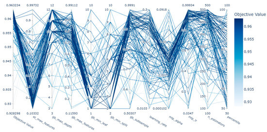
Figure 14.
Parallel coordinates’ visualization of hyperparameter tuning trials: parallel coordinate plot.
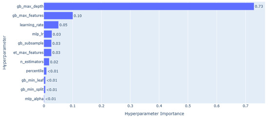
Figure 15.
Importance of hyperparameters in Gradient Boosting model optimization: hyperparameter importance plot.
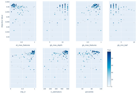
Figure 16.
Pairwise hyperparameter interaction effects on model performance: pairwise hyperparameter interaction plot.
6. Conclusions
This study proposed an advanced framework for flood susceptibility assessment by integrating explainable artificial intelligence (XAI) with AutoML optimization techniques. The Gradient Boosting (GB), Random Forest (RF), and Extreme Gradient Boosting (XGB) models were initially constructed using the Tree-based Pipeline Optimization Tool (TPOT), which employs evolutionary algorithms for pipeline generation. These models were subsequently fine-tuned using Optuna, a Bayesian optimization framework. Among them, the Optuna-optimized GB model achieved the highest performance (AUC = 0.966), confirming the effectiveness of a hybrid optimization strategy that combines global structural search with local parameter refinement. To enhance model transparency and trust, SHapley Additive exPlanations (SHAP) was applied for both global and local interpretability. SHAP summary and dependence plots identified elevation (DEM), distance to stream, stream density, slope, and built-up areas (lulc_7.0) as the most influential predictors of flood risk. Additionally, force and waterfall plots provided detailed instance-level explanations, illustrating how specific combinations of features contributed to individual predictions across a range of geospatial contexts. The results demonstrate that the integration of XAI and AutoML not only improves predictive performance but also facilitates interpretability, reproducibility, and decision support. This study contributes a replicable and adaptable modeling pipeline that can be extended to other natural hazard domains, offering scientific insights for flood mitigation planning, land use management, and spatial policy formulation.
Author Contributions
Conceptualization, K.N.; material, Y.L.; methods, K.N.; software, K.N.; validation, K.N.; formal analysis, K.N.; investigation, K.N.; data curation, K.N.; writing—original draft preparation, K.N.; writing, review and editing, Y.L., S.L., S.K. and S.Z.; visualization, K.N.; supervision, S.K.; project administration, Y.L. and S.L.; funding acquisition, S.L. All authors have read and agreed to the published version of the manuscript.
Funding
This research was supported by a grant (RS-2024-00402747) of Cooperative Research Method and Safety Management Technology in National Disaster funded by the Ministry of Interior and Safety (MOIS, Korea).
Data Availability Statement
The data presented in this study are available on request from the first author.
Acknowledgments
The authors express sincere appreciation to the Seoul Metropolitan Government for supplying the inundation inventory, which was crucial to this research.
Conflicts of Interest
The authors declare no conflicts of interest.
References
- Korea Research Institute for Human Settlements. KRIHS Issue Report No. 67; Korea Research Institute for Human Settlements: Sejong, Republic of Korea, 2022. [Google Scholar]
- Ha, G.; Jung, J. The Impact of Urbanization and Precipitation on Flood Damages. J. Korea Plan. Assoc. 2017, 52, 237–252. [Google Scholar] [CrossRef]
- Solomatine, D.P.; Ostfeld, A. Data-Driven Modelling: Some Past Experiences and New Approaches. J. Hydroinform. 2008, 10, 3–22. [Google Scholar] [CrossRef]
- Abedi, R.; Costache, R.; Shafizadeh-Moghadam, H.; Pham, Q.B. Flash-Flood Susceptibility Mapping Based on XGBoost, Random Forest and Boosted Regression Trees. Geocarto Int. 2022, 37, 5479–5496. [Google Scholar] [CrossRef]
- Chen, W.; Li, Y.; Xue, W.; Shahabi, H.; Li, S.; Hong, H.; Wang, X.; Bian, H.; Zhang, S.; Pradhan, B.; et al. Modeling Flood Susceptibility Using Data-Driven Approaches of Naïve Bayes Tree, Alternating Decision Tree, and Random Forest Methods. Sci. Total Environ. 2020, 701, 134979. [Google Scholar] [CrossRef]
- Pradhan, B.; Lee, S.R. Delineation of Landslide Hazard Areas on Penang Island, Malaysia, by using Frequency Ratio, Logistic Regression, and Artificial Neural Network Models. Environ. Earth Sci. 2010, 60, 1037–1054. [Google Scholar] [CrossRef]
- Aziz, K.; Rahman, A.; Fang, G.; Shrestha, S. Application of artificial neural networks in regional flood frequency analysis: A case study for Australia. Stoch. Environ. Res. Risk Assess. 2014, 28, 541–554. [Google Scholar] [CrossRef]
- Elsafi, S.H. Artificial neural networks (ANNs) for flood forecasting at Dongola Station in the River Nile, Sudan. Alex. Eng. J. 2014, 53, 655–662. [Google Scholar] [CrossRef]
- Sahana, M.; Rehman, S.; Sajjad, H.; Hong, H. Exploring Effectiveness of Frequency Ratio and Support Vector Machine Models in Storm Surge Flood Susceptibility Assessment: A Study of Sundarban Biosphere Reserve, India. Catena 2020, 189, 104450. [Google Scholar] [CrossRef]
- Tehrany, M.S.; Pradhan, B.; Jebur, M.N. Flood Susceptibility Mapping Using a Novel Ensemble Weights-of-Evidence and Support Vector Machine Models in GIS. J. Hydrol. 2014, 512, 332–343. [Google Scholar] [CrossRef]
- Tehrany, M.S.; Pradhan, B.; Mansor, S.; Ahmad, N. Flood Susceptibility Assessment Using GIS-Based Support Vector Machine Model with Different Kernel Types. Catena 2015, 125, 91–101. [Google Scholar] [CrossRef]
- Lyu, H.M.; Yin, Z.Y. Flood susceptibility prediction using tree-based machine learning models in the GBA. Sustain. Cities Soc. 2023, 97, 104744. [Google Scholar] [CrossRef]
- Ettinger, S.; Mounaud, L.; Magill, C.; Yao-Lafourcade, A.F.; Thouret, J.C.; Manville, V.; Negulescu, C.; Zuccaro, G.; De Gregorio, D.; Nardone, S. Building vulnerability to hydro-geomorphic hazards: Estimating damage probability from qualitative vulnerability assessment using logistic regression. J. Hydrol. 2016, 541, 563–581. [Google Scholar] [CrossRef]
- Bathrellos, G.; Karymbalis, E.; Skilodimou, H.; Gaki-Papanastassiou, K.; Baltas, E. Urban flood hazard assessment in the basin of Athens metropolitan city, Greece. Environ. Earth Sci. 2016, 75, 319. [Google Scholar] [CrossRef]
- Rahmati, O.; Pourghasemi, H.R.; Zeinivand, H. Flood susceptibility mapping using frequency ratio and weights-of-evidence models in the Golastan Province, Iran. Geocarto Int. 2016, 31, 42–70. [Google Scholar] [CrossRef]
- Bui, D.T.; Pradhan, B.; Nampak, H.; Bui, Q.T.; Tran, Q.A.; Nguyen, Q.P. Hybrid artificial intelligence approach based on neural fuzzy inference model and metaheuristic optimization for flood susceptibility modeling in a high-frequency tropical cyclone area using GIS. J. Hydrol. 2016, 540, 317–330. [Google Scholar] [CrossRef]
- Youssef, A.M.; Pradhan, B.; Sefry, S.A. Flash flood susceptibility assessment in Jeddah City (Kingdom of Saudi Arabia) using bivariate and multivariate statistical models. Environ. Earth Sci. 2016, 75, 12. [Google Scholar] [CrossRef]
- Amirebrahimi, S.; Rajabifard, A.; Mendis, P.; Ngo, T. A framework for a microscale flood damage assessment and visualization for a building using BIM–GIS integration. Int. J. Digit. Earth 2016, 9, 363–386. [Google Scholar] [CrossRef]
- Rahmati, O.; Zeinivand, H.; Besharat, M. Flood hazard zoning in Yasooj Region, Iran, using GIS and multi-criteria decision analysis. Geomat. Nat. Hazards Risk 2016, 7, 1000–1017. [Google Scholar] [CrossRef]
- Gu, H.; Gao, Y.; Fei, Y.; Sun, Y.; Tian, Y. Deep Learning and Hydrological Feature Constraint Strategies for Dam Detection: Global Application to Sentinel-2 Remote Sensing Imagery. Remote Sens. 2025, 17, 1194. [Google Scholar] [CrossRef]
- Mohsenifar, A.; Mohammadzadeh, A.; Jamali, S. Unsupervised Rural Flood Mapping from Bi-Temporal Sentinel-1 Images Using an Improved Wavelet-Fusion Flood-Change Index (IWFCI) and an Uncertainty-Sensitive Markov Random Field (USMRF) Model. Remote Sens. 2025, 17, 1024. [Google Scholar] [CrossRef]
- Askar, S.; Zeraat Peyma, S.; Yousef, M.M.; Prodanova, N.A.; Muda, I.; Elsahabi, M.; Hatamiafkoueieh, J. Flood Susceptibility Mapping Using Remote Sensing and Integration of Decision Table Classifier and Metaheuristic Algorithms. Water 2022, 14, 3062. [Google Scholar] [CrossRef]
- Rezaie, F.; Panahi, M.; Bateni, S.M.; Jun, C.; Neale, C.M.; Lee, S. Novel hybrid models by coupling support vector regression (SVR) with meta-heuristic algorithms (WOA and GWO) for flood susceptibility mapping. Nat. Hazards 2022, 114, 1247–1283. [Google Scholar] [CrossRef]
- Arora, A.; Arabameri, A.; Pandey, M.; Siddiqui, M.A.; Shukla, U.; Bui, D.T.; Mishra, V.N.; Bhardwaj, A. Optimization of state-of-the-art fuzzy-metaheuristic anfis-based machine learning models for flood susceptibility prediction mapping in the Middle Ganga Plain, India. Sci. Total Environ. 2021, 750, 141565. [Google Scholar] [CrossRef] [PubMed]
- Dodangeh, E.; Panahi, M.; Rezaie, F.; Lee, S.; Bui, D.T.; Lee, C.-W.; Pradhan, B. Novel hybrid intelligence models for flood-susceptibility prediction: Meta optimization of the gmdh and svr models with the genetic algorithm and harmony search. J. Hydrol. 2020, 590, 125423. [Google Scholar] [CrossRef]
- Bui, D.T.; Panahi, M.; Shahabi, H.; Singh, V.P.; Shirzadi, A.; Chapi, K.; Khosravi, K.; Chen, W.; Panahi, S.; Li, S. Novel hybrid evolutionary algorithms for spatial prediction of floods. Sci. Rep. 2018, 8, 15364. [Google Scholar] [CrossRef]
- Gao, Y.; Lu, H.; Zhang, Y.; Jin, H.; Wu, S.; Gao, Y.; Zhang, S. Evaluating Yangtze River Delta Urban Agglomeration flood risk using hybrid method of AutoML and AHP. Nat. Hazards Earth Syst. Sci. Discuss, 2024; in review. [Google Scholar] [CrossRef]
- He, F.; Liu, S.; Mo, X.; Wang, Z. Interpretable flash flood susceptibility mapping in Yarlung Tsangpo River Basin using H2O Auto-ML. Sci. Rep. 2025, 15, 1702. [Google Scholar] [CrossRef]
- Vincent, A.M.; Jidesh, P. An improved hyperparameter optimization framework for AutoML systems using evolutionary algorithms. Sci. Rep. 2023, 13, 4737. [Google Scholar] [CrossRef]
- Pradhan, B.; Lee, R.; Dikshit, A.; Kim, H. Spatial flood susceptibility mapping using an explainable artificial intelligence (XAI) model. Geosci. Front. 2023, 14, 6. [Google Scholar] [CrossRef]
- Zhang, Y.; Wei, Y.; Yao, R.; Sun, P.; Zhen, N.; Xia, X. Data Uncertainty of Flood Susceptibility Using Non-Flood Samples. Remote Sens. 2025, 17, 375. [Google Scholar] [CrossRef]
- Park, S.; Kim, J.; Kang, J. Exploring Optimal Deep Tunnel Sewer Systems to Enhance Urban Pluvial Flood Resilience in the Gangnam Region, South Korea. J. Environ. Manag. 2024, 357, 120762. [Google Scholar] [CrossRef]
- Ogden, F.L.; Raj Pradhan, N.; Downer, C.W.; Zahner, J.A. Relative importance of impervious area, drainage density, width function, and subsurface storm drainage on flood runoff from an urbanized catchment. Water Resour. Res. 2011, 47, 1–12. [Google Scholar] [CrossRef]
- Yang, H.; Yao, R.; Dong, L.; Sun, P.; Zhang, Q.; Wei, Y.; Sun, S.; Aghakouchak, A. Advancing flood susceptibility modeling using stacking ensemble machine learning: A multi-model approach. J. Geogr. Sci. 2024, 34, 1513–1536. [Google Scholar] [CrossRef]
- Yariyan, P.; Avand, M.; Abbaspour, R.A.; Torabi Haghighi, A.; Costache, R.; Ghorbanzadeh, O.; Janizadeh, S.; Blaschke, T. Flood susceptibility mapping using an improved analytic network process with statistical models. Geomat. Nat. Hazards Risk 2020, 11, 2282–2314. [Google Scholar] [CrossRef]
- Tehrany, M.S.; Jones, S.; Shabani, F. Identifying the essential flood conditioning factors for flood prone area mapping using machine learning techniques. Catena 2019, 175, 174–192. [Google Scholar] [CrossRef]
- Elshawi, M.; Sakr, S. Automated machine learning: State-of-the-art and open challenges. arXiv 2019, arXiv:1906.02287. [Google Scholar] [CrossRef]
- Fortin, F.-A.; Rainville, F.; Gardner, M.; Parizeau, M.; Gagne, C. DEAP: Evolutionary algorithms made easy. J. Mach. Learn. Res. 2012, 13, 2171–2175. [Google Scholar]
- Olson, R.S.; Moore, J.H. TPOT: A tree-based pipeline optimization tool for automating machine learning. JMLR Workshop Conf. Proc. 2016, 64, 66–74. [Google Scholar] [CrossRef]
- Almarzooq, H.; Bin Waheed, U. Automating hyperparameter optimization in geophysics with Optuna: A comparative study. Geophys. Prospect. 2024, 72, 1778–1788. [Google Scholar] [CrossRef]
- Li, Y.; Cao, Y.; Yang, J.; Wu, M.; Yang, A.; Li, J. Optuna-DFNN: An Optuna framework-driven deep fuzzy neural network for predicting sintering performance in big data. Alex. Eng. J. 2024, 97, 100–113. [Google Scholar] [CrossRef]
- Shapley, L.S. Stochastic games. Proc. Natl. Acad. Sci. USA 1953, 39, 1095–1100. [Google Scholar] [CrossRef]
- Aydin, H.E.; Iban, M.C. Predicting and analyzing flood susceptibility using boosting-based ensemble machine learning algorithms with SHapley Additive exPlanations. Nat. Hazards 2023, 116, 2957–2991. [Google Scholar] [CrossRef]
- Kim, Y.; Kim, Y. Explainable heat-related mortality with random forest and SHapley Additive exPlanations (SHAP) models. Sustain. Cities Soc. 2022, 79, 103677. [Google Scholar] [CrossRef]
- Tariq, A.; Yan, J.; Ghaffar, B.; Qin, S.; Mousa, B.G.; Sharifi, A.; Huq, M.E.; Aslam, M. Flash Flood Susceptibility Assessment and Zonation by Integrating Analytic Hierarchy Process and Frequency Ratio Model with Diverse Spatial Data. Water 2022, 14, 3069. [Google Scholar] [CrossRef]
- Ferri, C.; Hernández-Orallo, J.; Modroiu, R. An Experimental Comparison of Performance Measures for Classification. Pattern Recognit. Lett. 2009, 30, 27–38. [Google Scholar] [CrossRef]
- Tharwat, A. Classification Assessment Methods. Appl. Comput. Inform. 2018, 17, 168–192. [Google Scholar] [CrossRef]
- Lee, J.Y.; Kim, J.S. Detecting Areas Vulnerable to Flooding Using Hydrological-Topographic Factors and Logistic Regression. Appl. Sci. 2021, 11, 5652. [Google Scholar] [CrossRef]
- Lei, X.; Chen, W.; Panahi, M.; Falah, F.; Rahmati, O.; Uuemaa, E.; Kalantari, Z.; Ferreira, C.S.S.; Rezaie, F.; Tiefenbacher, J.P.; et al. Urban Flood Modeling Using Deep-Learning Approaches in Seoul, South Korea. J. Hydrol. 2021, 601, 126684. [Google Scholar] [CrossRef]
- Bersabe, J.T.; Jun, B.-W. The Machine Learning-Based Mapping of Urban Pluvial Flood Susceptibility in Seoul Integrating Flood Conditioning Factors and Drainage-Related Data. ISPRS Int. J. Geo Inf. 2025, 14, 57. [Google Scholar] [CrossRef]


Disclaimer/Publisher’s Note: The statements, opinions and data contained in all publications are solely those of the individual author(s) and contributor(s) and not of MDPI and/or the editor(s). MDPI and/or the editor(s) disclaim responsibility for any injury to people or property resulting from any ideas, methods, instructions or products referred to in the content. |
© 2025 by the authors. Licensee MDPI, Basel, Switzerland. This article is an open access article distributed under the terms and conditions of the Creative Commons Attribution (CC BY) license (https://creativecommons.org/licenses/by/4.0/).