Comparative Analysis of Machine Learning and Deep Learning Models for Individual Tree Structure Segmentation Using Terrestrial LiDAR Point Cloud Data

Abstract

This study aims to segment individual tree structures (stem, crown, and ground) from terrestrial LiDAR-derived point cloud data (PCD) and to compare the segmentation accuracy between two models: XGBoost (machine learning) and PointNet++ (deep learning). A total of 17 input features were categorized into spatial coordinates and normals, geometric structure features, and local distribution features. These were combined into four input configurations and evaluated under three downsampling conditions (2048, 4096, and 8192 points), resulting in 12 experimental setups. XGBoost achieved the highest stem segmentation F₁-score of 87.8% using all features with 8192 points, whereas Point-Net++ reached 92.1% using only spatial coordinates and normals with 4096 points. The analysis of missegmentation patterns showed that XGBoost frequently confused structures near stem-to-ground boundaries and around branch junctions, while PointNet++ occasionally missegmented complex regions between stems and crowns. Regarding processing time, XGBoost required 10 to 47 min across all conditions, whereas Point-Net++ required 49 min for the 2048-point condition and up to 168 min for 8192 points. Overall, XGBoost provided advantages in computational efficiency and in generating feature-importance scores, while PointNet++ outperformed XGBoost in segmentation accuracy and the recognition of structurally complex regions.

1. Introduction

Forests serve as stable sources of timber and major terrestrial carbon sinks, which are critical in climate change mitigation and biodiversity conservation [1]. National strategies to achieve carbon neutrality by 2050 have emphasized the need to quantitatively assess and systematically manage the carbon sequestration capacity of forests [2]. Accordingly, accurate estimation of tree-level biomass has emerged as a key requirement for sustainable forest management and climate policy implementation [3,4].

Conventional forest inventory methods typically involve measuring diameter at breast height (DBH) using tools such as D-tapes or calipers, and estimating tree height using clinometers or hypsometers, which rely on trigonometric calculations. Stem volume is subsequently derived from these DBH and height measurements [5]. However, these traditional approaches provide limited quantitative information on overall tree structure and morphology, and are susceptible to inter-observer variability, which compromises the precision and consistency of the data collected [6,7].

Precision forestry has gained prominence as a means to overcome these limitations and to efficiently acquire detailed tree-level information, fostering a transition toward data-driven and sensor-based forest assessment systems [8]. In line with this shift, forest policies in the Republic of Korea have promoted the integration of information and communications technology (ICT), including light detection and ranging (LiDAR), as well as the establishment of digital platforms for forest spatial information [9,10]. As a result, techniques for extracting and analyzing high-resolution three-dimensional data have become increasingly critical.

Among the key technologies that support precision forestry, terrestrial LiDAR scanning (TLS) has been widely adopted as an effective tool for acquiring detailed structural information. TLS captures the three-dimensional geometry of forest components by emitting laser pulses and recording their returns, producing highly accurate point cloud data (PCD) [11,12]. This non-contact method minimizes operator intervention and enables repeated measurements under consistent conditions. In particular, TLS is highly effective in capturing fine-scale stem geometry, which is essential for estimating tree volume and carbon stocks [13,14].

The PCD acquired via TLS contains comprehensive spatial information, including terrain, individual trees, understory vegetation, and other forest elements. To utilize this data effectively, segmentation plays a crucial role in isolating components of interest, such as stems, crowns, and ground surfaces [15,16].

While segmentation was traditionally performed manually, the growing volume of point cloud data and the inherent limitations of manual techniques—such as their time-consuming nature and susceptibility to analyst bias—have led to increasing demand for automated segmentation methods that ensure consistency and efficiency [17,18].

Recent advances in point cloud segmentation have increasingly adopted machine learning (ML) and deep learning (DL) techniques. ML models typically rely on predefined geometric features, such as curvature and normal vectors, for point-wise classification. In contrast, DL approaches—particularly point-based deep neural networks—automatically learn hierarchical structural patterns directly from raw point cloud data, eliminating the need for manual feature engineering [19,20,21,22]. These two paradigms differ substantially in feature handling, model architecture, and computational mechanisms, which in turn lead to distinct segmentation performance profiles and computational demands [23,24,25]. However, most previous studies have focused on evaluating the stem segmentation performance of individual models within either ML or DL frameworks, often applied in isolation [26,27,28].

Accordingly, this study aims to compare the stem segmentation performance of a representative machine learning model (XGBoost) and a deep learning model (PointNet++) under identical experimental conditions, using PCD acquired via TLS at the individual tree level.

The primary contributions of this study are threefold. First, we systematically compare XGBoost and PointNet++ for individual tree structure segmentation under strictly standardized experimental conditions, including identical input features, data preprocessing, and evaluation criteria. Second, we comprehensively evaluate four input feature configurations—spatial coordinates and normals, geometric structure features, local distribution features, and their combinations—ensuring fair and consistent comparisons across both models. Third, we implement a hybrid downsampling strategy that combines random sampling and Farthest Point Sampling (FPS), which leverages the advantages of both methods and allows robust evaluation across varying point densities. These aspects address limitations in previous research, where comparisons were often limited to a single model type or downsampling method, and provide a harmonized framework for objective performance assessment.

2. Materials and Methods

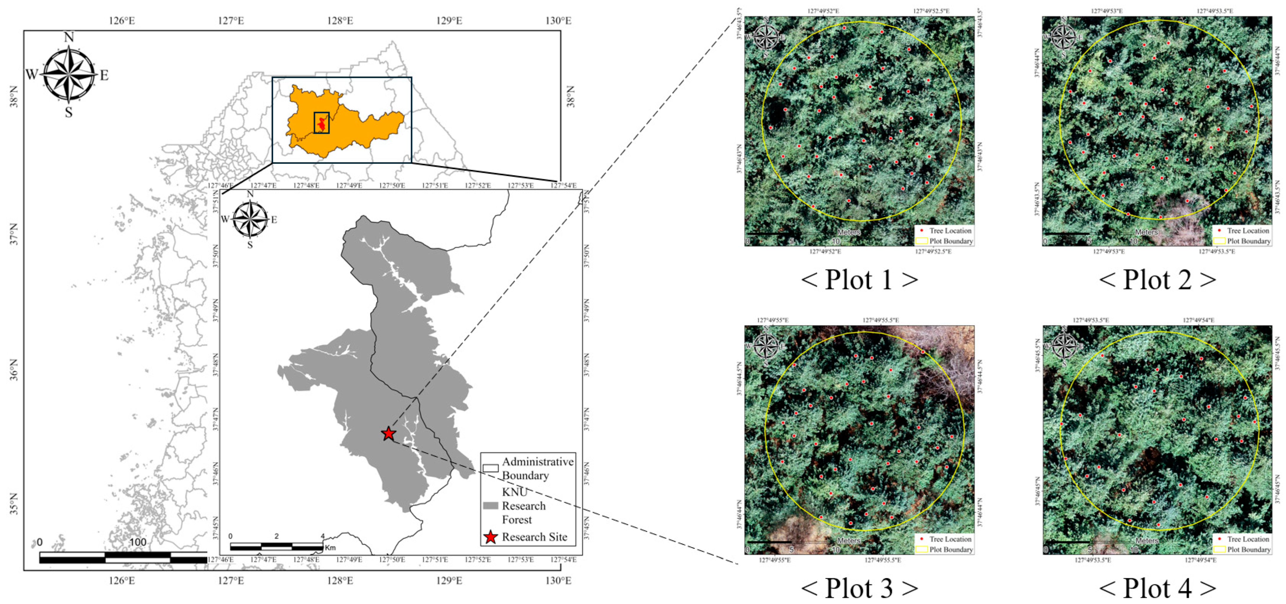
2.1. Study Area

This study was conducted in a Pinus koraiensis plantation within the Experimental Forest of Kangwon National University (KNU), spanning Bukbang-myeon, Hongcheon-gun, and Dongsan-myeon, Chuncheon-si, Gangwon Special Self-Governing Province, South Korea (Figure 1). The study area is classified as an artificial forest of age class V, with an average slope of approximately 20°. Due to its simple stand structure and uniform tree form, the site offers favorable conditions for the comparative analysis of structural segmentation algorithms.

Following the Korea National Forest Inventory (NFI) guidelines, four circular plots with a radius of 11.3 m were established [29]. The plots were selected to reflect variation in crown development, branch architecture, and site conditions within the same species. A total of 163 P. koraiensis trees were surveyed across the plots, with an average diameter at breast height (DBH) of 27.6 cm and an average tree height of 19.0 m (

Table 1. Stand structure characteristics of Pinus koraiensis by plot.

Plot	No. of Trees	DBH (cm)				Tree Height (m)
		Min	Max	Mean	Std	Min	Max	Mean	Std
1	52	12.0	45.0	26.4	6.3	14.9	24.7	18.5	1.8
2	46	13.6	48.4	27.0	6.7	13.4	23.0	18.6	2.0
3	36	13.9	43.1	28.1	8.1	14.7	22.5	20.0	1.9
4	29	12.6	51.3	29.5	8.5	14.7	29.2	20.3	2.3

).

2.2. Data Acquisition

PCD were acquired using a BLK360 terrestrial laser scanner (Leica Geosystems AG, Heerbrugg, Switzerland), which captures approximately 360,000 points per second within a maximum range of 60 m and offers a positional accuracy of approximately 4 mm at a distance of 10 m. For each plot, nine scan positions were used to minimize data occlusion. The scanner was placed at the plot center, at four equidistant points along the perimeter of the 11.3 m-radius circular plot, and at the four corners of an enclosing 16 m square (Figure 2a) [30].

Positional data for geometric correction were obtained using a Trimble R12i GNSS receiver (Trimble Inc., Sunnyvale, CA, USA), which provides survey-grade precision of 8 mm horizontally and 15 mm vertically [31,32]. A total of five ground control point (GCP) targets were installed: one at the center of the plot and four at the corners of the surrounding 16 m square. The GCP coordinates were measured using a VRS-RTK system under horizontal and vertical tolerances of less than 3 cm (Figure 2b).

After the procedure was routinized, each TLS scan position required about 5 min; thus, the nine positions per plot were completed in roughly 45 min. Each GCP target was logged for 60 epochs (≈1 min) until the horizontal and vertical tolerances of 3 cm were achieved.

2.3. Methodology

PCD were collected using TLS, and the plot-level PCD underwent preprocessing steps, including registration, georeferencing, and noise removal, to construct individual tree PCD. Each individual tree PCD was downsampled to 2048, 4096, and 8192 points, considering point density and computational efficiency. The dataset was divided into training, validation, and test sets in a 6:2:2 ratio.

To compare stem segmentation performance, two representative models, XGBoost for machine learning and PointNet++ for deep learning, were implemented under identical conditions. To evaluate the impact of input features on model performance, four combinations were configured by gradually adding different feature categories. These included spatial coordinates and normals (S), geometric structure features (G), and local distribution features (L). The resulting four input sets (S, S+G, S+L, and S+G+L) were applied consistently across both models. A total of 12 experimental datasets were created by combining these four input combinations with the three downsampling conditions (2048, 4096, and 8192 points). For each of these 12 datasets, confusion matrices were generated, and segmentation performance was quantitatively evaluated using standard performance metrics (Figure 3).

2.4. PCD Preprocessing and Individual Tree Data Construction

2.4.1. Point Cloud Registration and Geometric Correction

PCD collected from each scanning position was registered through a two-step process. Initial alignment was performed using Register360 Plus v2023.0.3 by matching feature points between adjacent scans and applying the cloud-to-cloud distance method, with the registration error constrained to less than 0.02 m. Fine alignment was then conducted using the Iterative Closest Point (ICP) algorithm in Cyclone v2023.0.1, resulting in a final registration error of under 0.005 m for each plot-level PCD [33,34].

Geometric correction was performed in CloudCompare by transforming the registered PCD into an absolute coordinate system using five GCPs installed per plot. The root mean square error (RMSE) of the transformation was maintained within 3 cm for all plots. The entire registration and georeferencing process for each plot required about 30 min.

2.4.2. Individual Tree Extraction

The extraction of individual trees was carried out through a semi-automated workflow designed for both efficiency and accuracy. First, the Cloth Simulation Filter (CSF), a widely used ground-filtering algorithm in CloudCompare, produced an initial coarse separation of ground and non-ground points [35]. This ground mask provided a reference height for locating points at breast height (1.2–1.3 m); their circular clusters were used to determine each stem center. Points within a 5 m radius around each stem center were then extracted to create an initial tree point cloud. To correct any CSF misclassifications and ensure data purity, we then performed meticulous manual refinement. During this step, residual non-target points, such as understory vegetation or sections of neighboring trees, were removed by visual inspection, yielding a clean, verified point cloud for every individual tree (Figure 4). This manual refinement process required about 10 min per tree.

2.4.3. PCD Noise Removal

PCD noise removal combined manual and automatic filtering. First, obvious noise in the upper canopy and lower ground areas was eliminated by visual inspection. Next, the Statistical Outlier Removal (SOR) algorithm was applied. SOR computes the mean distance from each point to its k nearest neighbors and removes points whose mean distance deviates from the global mean (μ) by more than a specified multiple of the standard deviation (σ) [36]. Guided by the parameter ranges recommended in earlier TLS studies [36,37], we tested combinations of k = 2, 4, 6, 8, 10 and σ = 1.5, 2, 2.5 on 20 randomly selected trees. The pairing k = 8 and σ = 2 offered the best trade-off between removing outliers and preserving fine-scale tree structure, and was therefore adopted for all subsequent processing. This automatic filtering required roughly 1 min per tree.

2.5. Label Data Construction for Tree Structure Segmentation

2.5.1. Manual Segmentation of Tree Structures

Tree structure segmentation was performed into three categories: stem, crown, and ground. These categories were chosen to clearly reflect the morphological differences of each structure and to enable effective learning of boundaries between categories during model training. Stem was defined as a cylindrical structure extending continuously along the vertical axis; branched or curved stems, as well as upper stem portions with lower point density, were still classified as stems provided that cross-sectional circularity was preserved. Crown comprised branches and foliage, where points are irregularly distributed [38,39]. Ground was defined as a surface exhibiting horizontal continuity and relatively uniform point density [40].

Manual segmentation was conducted by two trained annotators. Each individual tree point cloud was independently labeled and cross-checked at least three times; any discrepancies were resolved through consensus, ensuring consistent and verified annotations for all training and evaluation data. This entire manual annotation process required an average of 10 min per tree.

2.5.2. Dataset Construction Based on Downsampling Conditions

Individual tree PCD initially contained hundreds of thousands of points, requiring substantial computational resources for processing. To improve computational efficiency while preserving essential structural characteristics, each tree point cloud was downsampled to 2048, 4096, or 8192 points [41,42,43]. Downsampling was performed in two steps. First, a preliminary random sampling selected 10 times the target number of points. Then, Farthest Point Sampling (FPS) was applied to evenly distribute the final subset. This hybrid method addressed the spatial bias of pure random sampling and reduced the computational overhead associated with FPS alone [44,45].

During this process, a stratified sampling approach was adopted to achieve an approximate class distribution of 5:3:2 for stem, crown, and ground, respectively, aiming to provide a more balanced representation for model training. Each downsampled dataset was split into training (60%), validation (20%), and test (20%) subsets using stratified random sampling without replacement. The test set, excluded from the model training process, was used to objectively evaluate generalization performance [46,47].

2.6. Model Construction for Tree Structure Segmentation

2.6.1. Selection of Input Features

A total of 17 input features were used for tree structure segmentation and were grouped into three categories: spatial coordinates and normals (S), geometric structure features (G), and local distribution features (L). To compute the features in categories G and L, which rely on local context, a neighborhood was defined for each point using the K-nearest neighbors (KNN) method. The number of neighbors was set to K = 30, a value determined through preliminary tests to ensure the neighborhood was large enough to capture meaningful geometric and distributional patterns without oversmoothing fine details.

The spatial coordinates and normals (S) consist of the 3D coordinates (x, y, z) and their corresponding normal vectors (nx, ny, nz), which are used to identify structural directionality, such as the vertical alignment of stems and the horizontal characteristics of ground surfaces [48]. The geometric structure features (G) include linearity, planarity, sphericity, and verticality, derived from principal component analysis (PCA), which quantify the local shape around each point [40,49]. The local distribution features (L) include height range, height standard deviation, radial distance statistics, and the consistency of normal vector directions, contributing to the recognition of boundaries between structural components [50] (

Table 2. Computed point cloud features for tree structure segmentation.

Feature		Definition	Formula
spatial coordinates and normal (Dataset S)	x	3D x-coordinate of point	-
	y	3D y-coordinate of point	-
	z	3D z-coordinate of point	-
	$n_x$	x component of normal vector indicating surface direction	-
	$n_y$	y component of normal vector indicating surface direction	-
	$n_z$	z component of normal vector indicating surface direction	-
geometric structure features (Dataset G)	$L_{\lambda }$	Degree of linear arrangement of point cloud (Linearity)	${(\lambda }_1-{\lambda }_2)/{\lambda }_1$
	$P_{\lambda }$	Degree of planar arrangement of point cloud (Planarity)	${(\lambda }_2-{\lambda }_3)/{\lambda }_1$
	$S_{\lambda }$	Degree of spherical protrusion of point cloud (Sphericity)	${\lambda }_3/{\lambda }_1$
	$V$	Degree of vertical arrangement of point cloud (Verticality)	$1-n_z$
local distribution features (Dataset L)	$Z_{max}$	Maximum height of neighboring points	$\mathrm{m}\mathrm{a}\mathrm{x}(Z_1, Z_2, \dots , Z_k)$
	$Z_{min}$	Minimum height of neighboring points	$\mathrm{m}\mathrm{i}\mathrm{n}(Z_1, Z_2, \dots , Z_k)$
	$Z_{range}$	Height range of neighboring points	$Z_{max}-Z_{min}$
	$Z_{\sigma }$	Standard deviation of neighboring points’ heights	$\sqrt{{\displaystyle \frac{\sum _{i=1}^k{(z_i-\overline{z})}^2}{(k-1)}}}$
	$\overline{D}$	Average distance to neighboring points	${\displaystyle \frac{\sum _{i=1}^k{d}_i}{k}}$
	$D_{\sigma }$	Standard deviation of distances to neighboring points	$\sqrt{{\displaystyle \frac{\sum _{i=1}^k{(d_i-\overline{D})}^2}{(k-1)}}}$
	$N_c$	Normal vector consistency of neighboring points	${\displaystyle \frac{1}{k}}{\displaystyle \sum _{i=1}^k}\left|n_i·n\right|$

${\lambda }_1,{\lambda }_2,{\lambda }_3=Eigenvalues calculated from PCA({\lambda }_1\ge {\lambda }_2\ge {\lambda }_3)$, $n_z=z component of normal vector,k=number of neighboring points,$ $z_i=height of point i,\overline{z}=meanz-coordinate of neighboring points,$ $d_i=distance to point i,n_i=normal vector of i neighboring point$.

).

2.6.2. Model Selection and Training Configuration

To compare segmentation performance, this study employed XGBoost as a representative machine learning model and PointNet++ as a representative deep learning model. XGBoost is a tree-based ensemble algorithm that learns from pre-defined input features, whereas PointNet++ is a deep neural network that directly processes unordered point clouds. These models were chosen to enable a fair comparison across model families under identical input configurations and evaluation criteria.

XGBoost was selected because it has demonstrated superior performance and computational efficiency over traditional machine learning algorithms such as Random Forests and SVMs in point cloud classification and segmentation tasks [51,52]. Preliminary analyses on our dataset also indicated that XGBoost provided higher accuracy and shorter training time than Random Forests [53].

PointNet++ was chosen as one of the most widely adopted point-based deep learning architectures for 3D point cloud segmentation, offering robust performance across diverse datasets while directly processing unordered point sets [20,54]. Although more recent architectures (e.g., graph-based or transformer-based models) may offer further improvements, PointNet++ is commonly recognized as a standard baseline in the literature, ensuring fair and reproducible benchmarking in comparative studies.

XGBoost was implemented using a gradient boosting framework that iteratively refines residuals from previous decision trees [51]. Grid search was performed to optimize hyperparameters, including the number of estimators (500, 750, 1000), learning rate (0.001, 0.01, 0.1), and maximum tree depth (6, 8, 10) [55,56] (Figure 5a).

PointNet++ utilizes Set Abstraction and Feature Propagation layers to hierarchically learn both local and global features from 3D point clouds [20] (Figure 5b). Based on prior studies, training was conducted with a learning rate of 0.001, 200 epochs, and a batch size of 32 using the Adam optimizer [57,58,59,60]. Batch normalization and dropout were applied to improve training stability and generalization [61,62].

All model training and evaluation were conducted on a workstation equipped with an Intel Core i7-12700K (3.60 GHz, 12 cores) CPU, an NVIDIA GeForce RTX 3060 (12 GB) GPU, and 128 GB DDR4 RAM, using Python 3.9 and CUDA 12.1.

2.7. Evaluation of Tree Structure Segmentation Models

Model performance was evaluated using confusion matrices generated by comparing model predictions with the labeled test dataset [63]. For each class, the confusion matrix provided the counts of True Positives (TP), False Positives (FP), and False Negatives (FN). These counts were used to compute several quantitative metrics to assess segmentation performance, including Overall Accuracy, Precision, Recall, and F₁-score. Precision is the proportion of correctly predicted points among all points predicted as a given class, while Recall is the proportion of correctly predicted points among all actual points of that class [64]. The F₁-score, defined as the harmonic mean of Precision and Recall, was used to evaluate class-wise segmentation performance. The formulas for these metrics are presented in Equations (1)–(4).

$$Overall Accuracy(OA)={\displaystyle \frac{TP+TN}{TP+FP+TN+FN}}$$

(1)

$$Precision= {\displaystyle \frac{TP}{TP+FP}}$$

(2)

$$Recall= {\displaystyle \frac{TP}{TP+FN}}$$

(3)

$$F_1-score={\displaystyle \frac{2\times (Precision\times Recall)}{(Precision+Recall)}}$$

(4)

3. Results

3.1. Dataset Construction for Individual Tree Structure Segmentation

Each individual tree PCD contained an average of approximately 4.74 million points. Among the three structural components, the number of points was highest for the ground, followed by the crown and the stem. Although the stem had the fewest points, it exhibited the highest point density at 6970 pts/m², approximately 13.7 times greater than that of the crown and 7.7 times greater than that of the ground. This is attributed to the vertical and spatially continuous nature of stems, as well as their proximity to the TLS scanner. In contrast, the crown exhibited lower point density due to its complex and irregular structure, which caused occlusion and limited laser penetration through overlapping foliage and branches [65] (

Table 3. Summary statistics of point cloud distribution by tree structural components.

Structure	Number of Points (n = 163)				Point Density
	Min	Max	Mean	SD	Pts/m2
Overall Trees	265,148	13,252,547	4,742,683	2,654,630	1407
Stem	127,211	2,767,364	766,735	393,653	6970
Crown	63,204	4,950,873	872,765	694,291	508
Ground	74,733	8,891,581	3,103,183	1,975,605	908

).

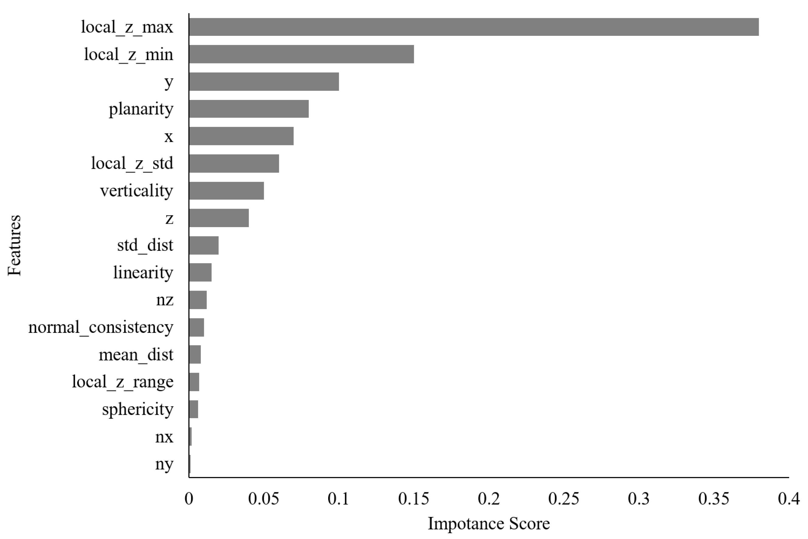
3.2. Hyperparameter Optimization and Feature Importance Analysis of XGBoost

The optimal hyperparameters for the XGBoost model were determined across all input feature combinations and downsampling conditions. The learning rate and maximum depth were consistently optimized at 0.01 and 6, respectively. The number of trees (n_estimators) was determined to be either 750 or 1000, depending on the configuration. Notably, segmentation accuracy was highest when 1000 trees were used under conditions with increased input dimensionality, such as the S+G and S+G+L combinations. This result suggests that a larger ensemble size was required to learn more complex boundaries introduced by additional features (

Table 4. Optimized hyperparameter settings for XGBoost under different input features and down-sampling conditions.

Downsampling	Dataset	n_Estimators (500, 750, 1000)	Max_Depth (6, 8, 10)	Learning_Rate (0.001, 0.01, 0.1)
2048	S	750	6	0.01
	S+G	750	6	0.01
	S+L	1000	6	0.01
	S+G+L	1000	6	0.01
4096	S	750	6	0.01
	S+G	750	6	0.01
	S+L	750	6	0.01
	S+G+L	1000	6	0.01
8192	S	750	6	0.01
	S+G	1000	6	0.01
	S+L	1000	6	0.01
	S+G+L	1000	6	0.01

). Under the best-performing condition (S+G+L with 8192 points), feature importance analysis revealed that local_z_max accounted for approximately 39% of the total relative importance. This feature, representing the maximum elevation within a local neighborhood, was effective in delineating boundaries between stems and crowns. The crown exhibited greater vertical variation, while the stem maintained a vertically continuous structure, making local_z_max a key indicator for structural distinction. In addition, local_z_min, which captures the minimum local elevation, was important for separating the lower stem from the ground. Among the spatial coordinates and normals (S), the x and y coordinates showed relatively high importance, likely due to their ability to capture horizontal spatial patterns across structural types. In contrast, the z coordinate was less influential, as relative height-based features such as local_z_max and local_z_min offered more discriminative power. Within the geometric structure features (G), planarity and verticality were the most important. Planarity contributed to identifying flat ground surfaces, while verticality helped distinguish upright stem structures (Figure 6). Among the normal vector components, nx and ny showed the lowest importance, contributing less than 0.01. This indicates that surface orientation alone was insufficient to capture structural differences, especially in the crown region, where directionality changes rapidly. Other irregular structure indicators, such as sphericity, local_z_range, and normal_consistency, also had low relative importance, suggesting a limited contribution to accurate boundary delineation between tree components [45,66].

3.3. Accuracy Evaluation Under Different Input Feature Combinations

Results showed that XGBoost maintained stable generalization performance across all input feature combinations and point sampling conditions, with the F₁-score difference between training and test sets remaining within 1.5 percentage points (

Table 5. Performance comparison of XGBoost and PointNet++ models under different input feature combinations and down-sampling conditions.

Model	Down Sampling	Dataset	Overall Accuracy (%)			F1-Score (%)			Runtime (min)
			Train	Val	Test	Train	Val	Test
XGBoost	2048	S	81.8	80.8	80.2	82.0	81.2	80.3	10
		S+G	84.9	84.3	83.9	85.4	84.9	84.4	12
		S+L	87.7	86.3	86.2	88.4	87.0	86.9	14
		S+G+L	88.3	87.3	87.1	89.0	87.9	87.7	16
	4096	S	82.0	80.8	80.2	82.2	81.3	80.4	17
		S+G	84.9	84.1	83.8	85.5	84.8	84.3	20
		S+L	87.4	86.1	86.2	88.1	86.8	86.9	22
		S+G+L	88.3	87.1	87.0	89.0	87.8	87.7	26
	8192	S	82.2	81.2	80.5	82.5	81.7	80.7	32
		S+G	85.3	84.4	84.2	85.9	85.1	84.7	35
		S+L	87.5	86.5	86.5	88.2	87.2	87.2	39
		S+G+L	88.3	87.4	87.3	89.0	88.2	88.0	47
PointNet++	2048	S	96.4	93.4	92.1	96.7	93.9	92.8	51
		S+G	92.8	86.9	85.2	92.7	87.9	86.3	59
		S+L	95.3	91.8	89.7	95.6	92.3	90.5	49
		S+G+L	91.4	84.8	83.8	92.1	86.1	85.1	55
	4096	S	95.6	93.4	92.2	96.3	93.9	93.0	65
		S+G	92.4	86.0	85.6	93.0	87.3	86.7	71
		S+L	94.8	90.8	89.3	95.2	91.6	90.4	65
		S+G+L	92.5	86.3	95.9	93.1	87.6	87.0	68
	8192	S	95.7	92.8	92.0	96.0	93.4	92.7	166
		S+G	91.9	84.9	83.6	97.8	86.3	85.1	168
		S+L	95.0	91.1	90.1	95.0	91.1	91.1	167
		S+G+L	92.1	86.0	85.4	92.7	87.2	86.5	167

). In contrast, PointNet++ demonstrated convergence between training and validation curves as training epochs increased. However, with increased input dimensionality, particularly in the S+G+L combination, the gap between training and validation accuracy widened, indicating that model performance decreased due to the increased complexity of variable interactions (Figure 7).

Based on the test set, PointNet++ achieved higher F₁-scores than XGBoost under all conditions. The highest accuracy was observed under the S condition with 4096 points, where PointNet++ reached an F₁-score of 93.0%, indicating effective learning of structural patterns using only spatial coordinates and normals. XGBoost showed its best performance under the S+G+L condition with 8192 points, achieving a maximum F₁-score of 88.0%. For both models, the S+L condition yielded higher accuracy than S+G, suggesting that local distribution features were more effective in identifying structural boundaries.

With respect to point density, PointNet++ showed greater sensitivity than XGBoost. The F₁-score variation of XGBoost remained within approximately 1 percentage point across different input sizes, indicating minimal impact of point density. In contrast, PointNet++ showed improved accuracy when increasing input size from 2048 to 4096 points, but accuracy declined slightly at 8192 points under the S, S+G, and S+G+L conditions.

This result suggests that segmentation performance may not continue to improve with increased point density under a fixed architecture. While overfitting of non-essential features is a plausible explanation—particularly under the S+G+L condition—other factors may also contribute. At 8192 points, the denser local neighborhoods may exceed the optimal receptive field of PointNet++’s Set Abstraction layers, leading to diluted feature representation or redundant processing. Additionally, increased computational noise or subtle outliers may further limit performance, particularly in the S dataset, which relies solely on spatial coordinates and normals. These factors indicate that there may be an optimal point resolution for a given PointNet++ configuration.

The runtime values in Table 5 represent the total processing time per condition, including training, validation, and test evaluation. XGBoost completed the entire process within 10 to 47 min, depending on input size, whereas PointNet++ required up to 168 min at 8192 points due to its more complex architecture. Although inference time per instance was not separately recorded, all evaluations were performed on downsampled PCD, and inference was completed within a few seconds per tree, suggesting practical feasibility for real-time or operational use [41,67].

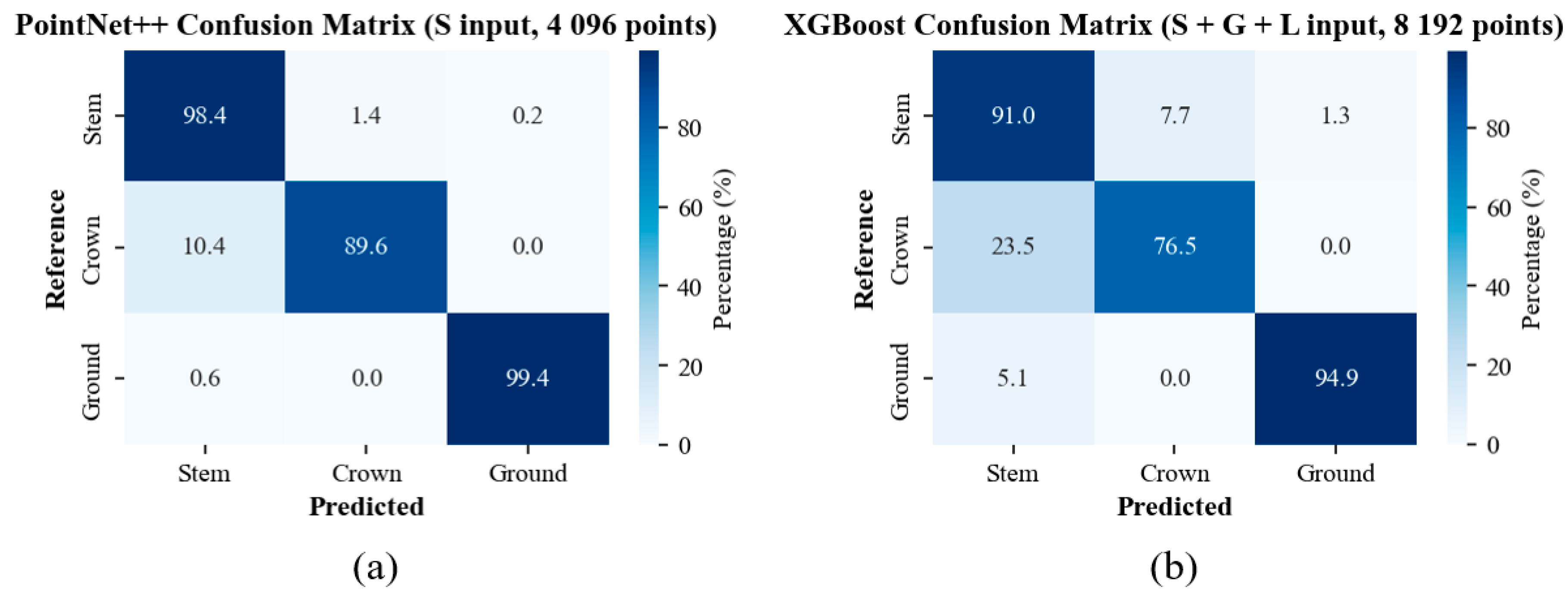
3.4. Class-Wise Tree Structure Segmentation Accuracy by ML and DL Models

The crown exhibited the lowest segmentation accuracy among the three structural categories. PointNet++ outperformed XGBoost by 7.0 percentage points in F₁-score. This improvement resulted from its capacity to learn localized features from grouped point structures, enabling it to accurately segment irregular branching patterns and discontinuous boundaries. This result aligns with previous studies reporting that PointNet++-based models achieve crown segmentation accuracy of approximately 90%, even under structurally complex conditions [39].

The ground class showed the highest segmentation accuracy in both models due to its planar geometry and clearly defined structural boundaries. PointNet++ achieved an F₁-score of 98.5%, while XGBoost achieved an F₁-score of 94.8%. The high accuracy of PointNet++ was due to its effective learning of spatial continuity and flat surface patterns [68]. Meanwhile, XGBoost also performed well by leveraging features such as local_z_min and planarity, which clearly characterize the structural features of ground points. In summary, PointNet++ demonstrated robust segmentation accuracy for both regular and irregular tree structures, particularly excelling in complex regions such as crowns. XGBoost was efficient in simpler or well-defined regions but was limited in its ability to distinguish fine-grained structural variations.

For a more direct comparison of model architectures, controlling for input data characteristics, we also evaluated the performance of both models under a matched input condition: 8192 points with S+G+L features (

Table 6. (a) Structure-wise segmentation performance of XGBoost and PointNet++ under their respective optimal input conditions. (b) Structure-wise segmentation performance comparison of XGBoost and PointNet++ under the matched input condition (8192 points, S+G+L).

Section	Model	Condition		Structure	Precision (%)	Recall (%)	F1-Score (%)
		Downsampling	Dataset
(a)	XGBoost	8192	S+G+L	Stem	84.7	81.1	87.8
				Crown	85.3	77.8	81.3
				Ground	97.6	92.2	94.8
	PointNet++	4096	S	Stem	93.4	90.9	92.1
				Crown	86.8	89.8	88.3
				Ground	97.7	99.3	98.5
(b)	XGBoost	8192	S+G+L	Stem	84.7	81.1	87.8
				Crown	85.3	77.8	81.3
				Ground	97.6	92.2	94.8
	PointNet++	8192	S+G+L	Stem	87.5	82.5	84.9
				Crown	77.6	80.7	79.1
				Ground	91.8	99.5	95.5

b). This specific condition represents XGBoost’s optimal setup and serves as a comprehensive input for PointNet++. Under this matched condition, PointNet++ achieved F₁-scores of 84.9% for stem, 79.1% for crown, and 95.5% for ground. When compared directly with XGBoost’s performance under the identical 8192-point, S+G+L condition, which had F₁-scores of 87.8% for stem, 81.3% for crown, and 94.8% for ground, PointNet++ showed a slight decrease in F₁-score for stem segmentation, with 84.9% compared to 87.8%. However, PointNet++ maintained a higher F₁-score for ground segmentation, achieving 95.5% compared to 94.8%. Crown segmentation performance was slightly lower for PointNet++ in this matched condition, 79.1% compared to 81.3%. This controlled comparison highlights that while PointNet++ demonstrates superior performance under its own optimized conditions (e.g., simpler S features), its architectural advantage might be less pronounced or even vary by class when directly compared with XGBoost on its most complex, optimal feature set. This implies that the benefits of PointNet++’s direct point processing may be more significant with basic spatial information or moderate densities, whereas XGBoost can effectively leverage highly engineered features from denser point clouds to achieve competitive results in certain classes.

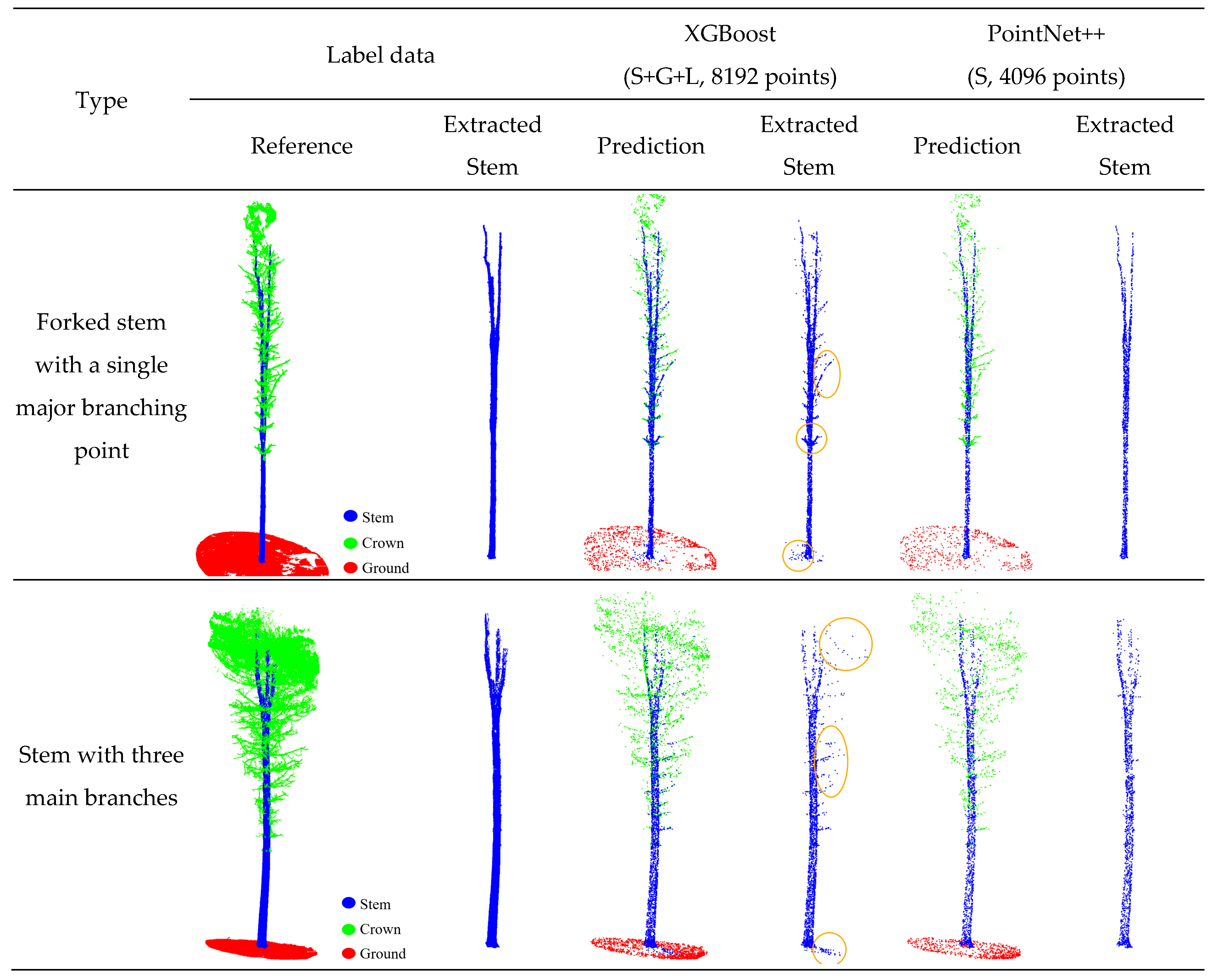
3.5. Analysis of Missegmentation Cases in Tree Structure Segmentation

An analysis of missegmentation cases revealed common error patterns related to structural characteristics and model-specific tendencies, visually illustrated in Figure 8 and quantified by the confusion matrices in Figure 9. For both models, the most frequent error was the confusion between the stem and crown classes, particularly in the upper stem region where major branching occurs.

This issue was most pronounced in the XGBoost model. Its most significant error was the missegmentation of crown points into the stem class, affecting 23.5% of all crown points (Figure 9b). This error is visually evident in Figure 8. A second notable error was the missegmentation of 5.1% of ground points into the stem class near the boundary. This may be due to the similar point density and spatial continuity in this transition zone, making the boundary ambiguous for the feature-based model. These limitations are consistent with findings from previous studies on the challenges of segmenting connected structures using tree-based models [69].

In contrast, the PointNet++ model demonstrated more reliable segmentation overall. While it also exhibited some confusion between crown and stem, it was significantly more robust than XGBoost in this regard, with the missegmentation of crown points into the stem class occurring at a lower rate of 10.4% (Figure 9a). This superior performance is attributed to its ability to capture local spatial relationships, allowing it to better recognize fine-grained structural differences. However, as illustrated in Figure 8, occasional errors still occurred in areas with complex branching geometry, which aligns with previously reported observations of PointNet++ performance in structurally complex tree regions [39].

4. Discussion

The comparative results between XGBoost and PointNet++ reveal distinct strengths rooted in their underlying algorithmic architectures. PointNet++ consistently outperformed XGBoost in segmentation accuracy, particularly for structurally complex classes such as the crown and stem. Its ability to capture local geometric continuity contributed to high precision, even under reduced input conditions. However, the model exhibited signs of overfitting under high-dimensional input combinations, particularly with the inclusion of both geometric and local distribution features. This sensitivity, along with the increased computational cost observed at higher point densities, suggests that deep learning models may require careful optimization for scalable deployment in operational forestry settings.

In contrast, XGBoost demonstrated stable generalization performance across all downsampling conditions, with minimal variation in accuracy and relatively short processing time. Its performance was strongly influenced by the composition of input features, with local elevation and geometric variables contributing most significantly. While its tree-based structure was effective in identifying regular and clearly bounded structures such as the ground, it showed limitations in distinguishing ambiguous boundaries between overlapping classes, such as the stem-crown interface.

These findings underscore the importance of selecting a segmentation model according to data characteristics, structural complexity, and computational constraints. We acknowledge two main limitations of this study: the analysis was conducted on a single species to ensure a clear methodological comparison, and the evaluation was limited to one representative model from each paradigm. Additionally, this study did not incorporate rigorous statistical analyses to quantify the variability or statistical significance of the observed performance differences between models, relying instead on direct comparisons of performance metrics from a single evaluation. Future work should therefore apply this framework to more diverse forest types, including mixed-species and broadleaf stands, and broaden the benchmark to cover additional algorithms, such as other ensemble methods and newer deep learning architectures, and critically, integrate rigorous statistical methodologies (e.g., k-fold cross-validation with confidence intervals and significance testing) to provide a more robust assessment of model performance. To enhance its utility as benchmark data for large-scale remote sensing (e.g., ALS or SAR), future work must also develop automatic metrics for self-standing validation, such as stem-center offsets (ΔX, ΔY, ΔZ) and class-wise IoU. In addition, the recent emergence of public benchmark datasets, such as For-species20K, FOR-Instance, and the TLSForests repository, offers opportunities to evaluate model generalizability across different sensor types (e.g., static TLS, mobile MLS, or UAV-borne LiDAR) and forest structures. These resources provide standardized, annotated point clouds from diverse environments and acquisition setups, supporting cross-study comparison and model benchmarking under heterogeneous conditions [18,70,71]. Hybrid frameworks that combine the computational efficiency of feature-based machine learning with the spatial-learning capability of deep neural networks may also offer a promising path toward both precision and operational viability in forest-structure segmentation.

5. Conclusions

This study conducted a comparative evaluation of the XGBoost and PointNet++ models for segmenting tree structures at the individual tree level using PCD acquired through TLS. All models were tested under identical conditions with consistent input configurations, including spatial coordinates and normals, geometric structure features, and local distribution features. Model performance was assessed based on segmentation accuracy across different downsampling conditions, input feature combinations, and computational efficiency. The two models exhibited clear differences in their learning mechanisms, input processing methods, and performance stability. PointNet++, as a deep learning model, achieved high segmentation accuracy even with relatively simple input features and showed strong capability in recognizing complex structural boundaries and transition areas.

In contrast, XGBoost offered strengths in computational efficiency and in providing feature-importance scores. These findings suggest that deep learning models are more suitable for tasks requiring detailed structural recognition, while machine learning models may be more effective in settings where rapid processing and transparent feature ranking are priorities. Overall, the results provide practical guidance for selecting appropriate models according to data conditions and operational constraints in the development and application of tree structure segmentation systems.

References

1. Psistaki, K.; Tsantopoulos, G.; Paschalidou, A.K. An overview of the role of forests in climate change mitigation. Sustainability 2024, 16, 6089. [Google Scholar] [CrossRef]
2. Jiao, Y.; Wang, D.; Yao, X.; Wang, S.; Chi, T.; Meng, Y. Forest emissions reduction assessment using optical satellite imagery and space LiDAR fusion for carbon stock estimation. Remote Sens. 2023, 15, 1410. [Google Scholar] [CrossRef]
3. Sparks, A.M.; Smith, A.M. Accuracy of a lidar-based individual tree detection and attribute measurement algorithm developed to inform forest products supply chain and resource management. Forests 2021, 13, 3. [Google Scholar] [CrossRef]
4. Ko, C.U.; Kang, J.T.; Park, J.M.; Lee, M.W. Assessing forest resources with terrestrial and backpack LiDAR: A case study on leaf-on and leaf-off conditions in Gari Mountain, Hongcheon, Republic of Korea. Forests 2024, 15, 2230. [Google Scholar] [CrossRef]
5. Bauwens, S.; Bartholomeus, H.; Calders, K.; Lejeune, P. Forest inventory with terrestrial LiDAR: A comparison of static and hand-held mobile laser scanning. Forests 2016, 7, 127. [Google Scholar] [CrossRef]
6. Kim, D.Y.; Choi, Y.W.; Lee, G.S.; Cho, G.S. Extracting individual number and height of tree using airborne LiDAR data. J. Cadastre Land Inf. 2016, 46, 87–100. [Google Scholar]
7. Seo, S.H.; Park, K.M.; Jung, T.Y. Study on tree volume measurement using terrestrial and airborne laser scanners. J. Korean Inst. Landsc. Archit. 2024, 52, 42–52. [Google Scholar] [CrossRef]
8. Woo, H.; Cho, S.; Jung, G.; Park, J. Precision forestry using remote sensing techniques: Opportunities and limitations of remote sensing application in forestry. Korean J. Remote Sens. 2019, 35, 1067–1082. [Google Scholar] [CrossRef]
9. Korea Forest Service. Forest Master Plans, 6th ed.; Korea Forest Service: Daejeon, Republic of Korea, 2018; p. 27. [Google Scholar]
10. Jo, S.H.; Ban, S.H.; Lee, H.J.; Choi, S.K. Individual tree detection in natural forest using high density airborne laser scanning. J. Korean Soc. Geospat. Inf. Sci. 2023, 31, 29–38. [Google Scholar] [CrossRef]
11. Raumonen, P.; Casella, E.; Calders, K.; Murphy, S.; Åkerblom, M.; Kaasalainen, M. Massive-scale tree modelling from TLS data. ISPRS Ann. Photogramm. Remote Sens. Spat. Inf. Sci 2015, II-3/W4, 189–196. [Google Scholar] [CrossRef]
12. Sheppard, J.; Morhart, C.; Hackenberg, J.; Spiecker, H. Terrestrial laser scanning as a tool for assessing tree growth. iForest 2017, 10, 172–179. [Google Scholar] [CrossRef]
13. Boucher, P.B.; Paynter, I.; Orwig, D.A.; Valencius, I.; Schaaf, C. Sampling forests with terrestrial laser scanning. Ann. Bot. 2021, 128, 689–708. [Google Scholar] [CrossRef] [PubMed]
14. Campos, M.B.; Litkey, P.; Wang, Y.; Chen, Y.; Hyyti, H.; Hyyppä, J.; Puttonen, E. A long-term terrestrial laser scanning measurement station to continuously monitor structural and phenological dynamics of boreal forest canopy. Front. Plant Sci. 2021, 11, 606752. [Google Scholar] [CrossRef]
15. Hackenberg, J.; Spiecker, H.; Calders, K.; Disney, M.; Raumonen, P. SimpleTree—An efficient open source tool to build tree models from TLS clouds. Forests 2015, 6, 4245–4294. [Google Scholar] [CrossRef]
16. Wang, D.; Liang, X.; Mofack, G.I.; Martin-Ducup, O. Individual tree extraction from terrestrial laser scanning data via graph pathing. For. Ecosyst. 2021, 8, 67. [Google Scholar] [CrossRef]
17. De Paula Pires, R.; Olofsson, K.; Persson, H.J.; Lindberg, E.; Holmgren, J. Individual tree detection and estimation of stem attributes with mobile laser scanning along boreal forest roads. ISPRS J. Photogramm. Remote Sens. 2022, 187, 211–224. [Google Scholar] [CrossRef]
18. Wilkes, P.; Disney, M.; Armston, J.; Bartholomeus, H.; Bentley, L.; Brede, B.; Burt, A.; Calders, K.; Chavana-Bryant, C.; Clewley, D.; et al. TLS2trees: A scalable tree segmentation pipeline for TLS data. Methods Ecol. Evol. 2023, 14, 3083–3099. [Google Scholar] [CrossRef]
19. Qi, C.R.; Su, H.; Mo, K.; Guibas, L.J. PointNet: Deep learning on point sets for 3D classification and segmentation. In Proceedings of the IEEE Conference on Computer Vision and Pattern Recognition (CVPR), Honolulu, HI, USA, 21–26 July 2017; pp. 652–660. [Google Scholar] [CrossRef]
20. Qi, C.R.; Yi, L.; Su, H.; Guibas, L.J. PointNet++: Deep hierarchical feature learning on point sets in a metric space. Adv. Neural Inf. Process. Syst. 2017, 30, 5105–5114. [Google Scholar] [CrossRef]
21. Su, Z.; Li, S.; Liu, H.; Liu, Y. Extracting wood point cloud of individual trees based on geometric features. IEEE Geosci. Remote Sens. Lett. 2019, 16, 1294–1298. [Google Scholar] [CrossRef]
22. Neuville, R.; Bates, J.S.; Jonard, F. Estimating forest structure from UAV-mounted LiDAR point cloud using machine learning. Remote Sens. 2021, 13, 352. [Google Scholar] [CrossRef]
23. Gharineiat, Z.; Tarsha Kurdi, F.; Campbell, G. Review of automatic processing of topography and surface feature identification LiDAR data using machine learning techniques. Remote Sens. 2022, 14, 4685. [Google Scholar] [CrossRef]
24. Windrim, L.; Bryson, M. Detection, segmentation, and model fitting of individual tree stems from airborne laser scanning of forests using deep learning. Remote Sens. 2020, 12, 1469. [Google Scholar] [CrossRef]
25. Daif, H.; Marzouk, M. Point cloud classification and part segmentation of steel structure elements. Neural Comput. Appl. 2025, 37, 4387–4407. [Google Scholar] [CrossRef]
26. Itakura, K.; Miyatani, S.; Hosoi, F. Estimating tree structural parameters via automatic tree segmentation from LiDAR point cloud data. IEEE J. Sel. Top. Appl. Earth Obs. Remote Sens. 2021, 15, 555–564. [Google Scholar] [CrossRef]
27. Zhang, W.; Wan, P.; Wang, T.; Cai, S.; Chen, Y.; Jin, X.; Yan, G. A novel approach for the detection of standing tree stems from plot-level terrestrial laser scanning data. Remote Sens. 2019, 11, 211. [Google Scholar] [CrossRef]
28. Shao, J.; Lin, Y.C.; Wingren, C.; Shin, S.Y.; Fei, W.; Carpenter, J.; Habib, A.; Fei, S. Large-scale inventory in natural forests with mobile LiDAR point clouds. Sci. Remote Sens. 2024, 10, 100168. [Google Scholar] [CrossRef]
29. Korea Forest Service and Korea Forestry Promotion Institute. The 8th National Forest Inventory and Forest Health Monitoring. -Field Manual-; Korea Forestry Promotion Institute: Seoul, Republic of Korea, 2021; pp. 7–8. [Google Scholar]
30. National Institute of Forest Science (NIFoS). Guidelines for Using Terrestrial LiDAR for Digital Forest Resource Inventory; NIFoS: Seoul, Republic of Korea, 2022. [Google Scholar]
31. Pavelka, K.; Zahradnik, D.; Sedina, J. New measurement methods for structure deformation and objects exact dimension determination. IOP Conf. Ser. Earth Environ. Sci. 2021, 906, 012060. [Google Scholar] [CrossRef]
32. Lopatin, E.; Vaatainen, K.; Kukko, A.; Kaartinen, H.; Hyyppä, J.; Holmström, E.; Sikanen, L.; Nuutinen, Y.; Routa, J. Unlocking digitalization in forest operations with viewshed analysis to improve GNSS positioning accuracy. Forests 2023, 14, 689. [Google Scholar] [CrossRef]
33. Panella, F.; Roecklinger, N.; Vojnovic, L.; Loo, Y.; Boehm, J. Cost–benefit analysis of rail tunnel inspection for photogrammetry and laser scanning. ISPRS Arch. Photogramm. Remote Sens. Spat. Inf. Sci. 2020, XLIII-B2-2020, 1137–1144. [Google Scholar] [CrossRef]
34. Zhang, J.; Wang, J.; Cheng, F.; Ma, W.; Liu, Q.; Liu, G. Natural forest ALS–TLS point cloud data registration without control points. J. For. Res. 2023, 34, 809–820. [Google Scholar] [CrossRef]
35. Zhang, W.; Qi, J.; Wan, P.; Wang, H.; Xie, D.; Wang, X.; Yan, G. An easy-to-use airborne LiDAR data filtering method based on cloth simulation. Remote Sens. 2016, 8, 501. [Google Scholar] [CrossRef]
36. Duan, D.; Deng, Y.; Zhang, J.; Wang, J.; Dong, P. Influence of VF and SOR-filtering methods on tree height inversion using unmanned aerial vehicle LiDAR data. Drones 2024, 8, 119. [Google Scholar] [CrossRef]
37. Tai, H.; Xia, Y.; Yan, M.; Li, C.; Kong, X. Construction of artificial forest point clouds by laser SLAM technology and estimation of carbon storage. Appl. Sci. 2022, 12, 10838. [Google Scholar] [CrossRef]
38. Wang, D.; Momo Takoudjou, S.; Casella, E. LeWoS: A universal leaf–wood classification method to facilitate the 3D modelling of large tropical trees using terrestrial LiDAR. Methods Ecol. Evol. 2020, 11, 376–389. [Google Scholar] [CrossRef]
39. Kim, D.H.; Ko, C.U.; Kim, D.G.; Kang, J.T.; Park, J.M.; Cho, H.J. Automated segmentation of individual tree structures using deep learning over LiDAR point cloud data. Forests 2023, 14, 1159. [Google Scholar] [CrossRef]
40. Tarsha Kurdi, F.; Gharineiat, Z.; Lewandowicz, E.; Shan, J. Modeling the geometry of tree trunks using LiDAR data. Forests 2024, 15, 368. [Google Scholar] [CrossRef]
41. Liu, B.; Chen, S.; Huang, H.; Tian, X. Tree species classification of backpack laser scanning data using the PointNet++ point cloud deep learning method. Remote Sens. 2022, 14, 3809. [Google Scholar] [CrossRef]
42. Pan, L.; Chen, X.; Cai, Z.; Zhang, J.; Zhao, H.; Yi, S.; Liu, Z. Variational relational point completion network for robust 3D classification. IEEE Trans. Pattern Anal. Mach. Intell. 2023, 45, 11340–11351. [Google Scholar] [CrossRef]
43. Sun, P.; Yuan, X.; Li, D. Classification of individual tree species using UAV LiDAR based on transformer. Forests 2023, 14, 484. [Google Scholar] [CrossRef]
44. Hu, Q.; Yang, B.; Xie, L.; Rosa, S.; Guo, Y.; Wang, Z.; Trigoni, N.; Markham, A. Learning semantic segmentation of large-scale point clouds with random sampling. IEEE Trans. Pattern Anal. Mach. Intell. 2021, 44, 8338–8354. [Google Scholar] [CrossRef]
45. Han, T.; Sánchez-Azofeifa, G.A. A deep learning time series approach for leaf and wood classification from terrestrial LiDAR point clouds. Remote Sens. 2022, 14, 3157. [Google Scholar] [CrossRef]
46. Van den Broeck, W.A.J.; Terryn, L.; Cherlet, W.; Cooper, Z.T.; Calders, K. Three-dimensional deep learning for leaf–wood segmentation of tropical tree point clouds. ISPRS Arch. Photogramm. Remote Sens. Spat. Inf. Sci. 2023, XLVIII-1/W2-2023, 765–770. [Google Scholar] [CrossRef]
47. Zhong, H.; Zhang, Z.; Liu, H.; Wu, J.; Lin, W. Individual tree species identification for complex coniferous and broad-leaved mixed forests based on deep learning combined with UAV LiDAR data and RGB images. Forests 2024, 15, 293. [Google Scholar] [CrossRef]
48. Weinmann, M.; Urban, S.; Hinz, S.; Jutzi, B.; Mallet, C. Distinctive 2D and 3D features for automated large-scale scene analysis in urban areas. Comput. Graph. 2015, 49, 47–57. [Google Scholar] [CrossRef]
49. Chen, M.; Liu, X.; Pan, J.; Mu, F.; Zhao, L. Stem detection from terrestrial laser scanning data with features selected via stem-based evaluation. Forests 2023, 14, 2035. [Google Scholar] [CrossRef]
50. Jiang, T.; Zhang, Q.; Liu, S.; Liang, C.; Dai, L.; Zhang, Z.; Wang, Y. LWSNet: A point-based segmentation network for leaf–wood separation of individual trees. Forests 2023, 14, 1303. [Google Scholar] [CrossRef]
51. Xianyi, W.; Yanqiu, X.; Haotian, Y.; Tao, X.; Su, S. TLS point cloud classification of forest based on nearby geometric features. J. Beijing For. Univ. 2019, 41, 138–146. [Google Scholar] [CrossRef]
52. Rust, S.; Stoinski, B. Enhancing Tree Species Identification in Forestry and Urban Forests through Light Detection and Ranging Point Cloud Structural Features and Machine Learning. Forests 2024, 15, 188. [Google Scholar] [CrossRef]
53. Han, T.; Sánchez-Azofeifa, G.A. Extraction of liana stems using geometric features from terrestrial laser scanning point clouds. Remote Sens. 2022, 14, 4039. [Google Scholar] [CrossRef]
54. Fan, Z.; Wei, J.; Zhang, R.; Zhang, W. Tree species classification based on PointNet++ and airborne laser survey point cloud data enhancement. Forests 2023, 14, 1246. [Google Scholar] [CrossRef]
55. Moorthy, S.M.K.; Bao, Y.; Calders, K.; Schnitzer, S.A.; Verbeeck, H. Semi-automatic extraction of liana stems from terrestrial LiDAR point clouds of tropical rainforests. ISPRS J. Photogramm. Remote Sens. 2019, 154, 114–126. [Google Scholar] [CrossRef]
56. Yu, J.W.; Yoon, Y.W.; Baek, W.K.; Jung, H.S. Forest vertical structure mapping using two-seasonal optic images and LiDAR DSM acquired from UAV platform through random forest, XGBoost, and support vector machine approaches. Remote Sens. 2021, 13, 4282. [Google Scholar] [CrossRef]
57. Luo, Z.; Zhang, Z.; Li, W.; Chen, Y.; Wang, C.; Nurunnabi, A.A.M.; Li, J. Detection of individual trees in UAV LiDAR point clouds using a deep learning framework based on multichannel representation. IEEE Trans. Geosci. Remote Sens. 2021, 60, 5701715. [Google Scholar] [CrossRef]
58. Han, J.W.; Synn, D.J.; Kim, T.H.; Chung, H.C.; Kim, J.K. Feature based sampling: A fast and robust sampling method for tasks using 3D point cloud. IEEE Access 2022, 10, 58062–58070. [Google Scholar] [CrossRef]
59. Lee, Y.K.; Lee, S.J.; Lee, J.S. Comparison and evaluation of classification accuracy for Pinus koraiensis and Larix kaempferi based on LiDAR platforms and deep learning models. Korean J. For. Sci. 2023, 112, 195–208. [Google Scholar] [CrossRef]
60. Ge, B.; Chen, S.; He, W.; Qiang, X.; Li, J.; Teng, G.; Huang, F. Tree Completion Net: A novel vegetation point clouds completion model based on deep learning. Remote Sens. 2024, 16, 3763. [Google Scholar] [CrossRef]
61. Soydaner, D. A comparison of optimization algorithms for deep learning. Int. J. Pattern Recognit. Artif. Intell. 2020, 34, 2052013. [Google Scholar] [CrossRef]
62. Kandel, I.; Castelli, M. The effect of batch size on the generalizability of the convolutional neural networks on a histopathology dataset. ICT Express 2020, 6, 312–315. [Google Scholar] [CrossRef]
63. Münzinger, M.; Prechtel, N.; Behnisch, M. Mapping the urban forest in detail: From LiDAR point clouds to 3D tree models. Urban For. Urban Green. 2022, 74, 127637. [Google Scholar] [CrossRef]
64. Cherlet, W.; Cooper, Z.; Van Den Broeck, W.A.; Disney, M.; Origo, N.; Calders, K. Benchmarking instance segmentation in terrestrial laser scanning forest point clouds. In Proceedings of the IGARSS 2024—2024 IEEE International Geoscience and Remote Sensing Symposium, Athens, Greece, 7–12 July 2024; pp. 4511–4515. [Google Scholar] [CrossRef]
65. Mathes, T.; Seidel, D.; Häberle, K.H.; Pretzsch, H.; Annighöfer, P. What are we missing? Occlusion in laser scanning point clouds and its impact on the detection of single-tree morphologies and stand structural variables. Remote Sens. 2023, 15, 450. [Google Scholar] [CrossRef]
66. Ou, J.; Tian, Y.; Zhang, Q.; Xie, X.; Zhang, Y.; Tao, J.; Lin, J. Coupling UAV hyperspectral and LiDAR data for mangrove classification using XGBoost in China’s Pinglu Canal Estuary. Forests 2023, 14, 1838. [Google Scholar] [CrossRef]
67. Kulicki, M.; Cabo, C.; Trzciński, T.; Będkowski, J.; Stereńczak, K. Artificial intelligence and terrestrial point clouds for forest monitoring. Curr. For. Rep. 2024, 11, 5. [Google Scholar] [CrossRef]
68. Ma, Z.; Dong, Y.; Zi, J.; Xu, F.; Chen, F. Forest-PointNet: A deep learning model for vertical structure segmentation in complex forest scenes. Remote Sens. 2023, 15, 4793. [Google Scholar] [CrossRef]
69. Moorthy, S.M.K.; Calders, K.; Vicari, M.B.; Verbeeck, H. Improved supervised learning-based approach for leaf and wood classification from LiDAR point clouds of forests. IEEE Trans. Geosci. Remote Sens. 2020, 58, 3057–3070. [Google Scholar] [CrossRef]
70. Puliti, S.; Pearse, G.; Surový, P.; Wallace, L.; Hollaus, M.; Wielgosz, M.; Astrup, R. For-instance: A uav laser scanning benchmark dataset for semantic and instance segmentation of individual trees. arXiv 2023, arXiv:2309.01279. [Google Scholar] [CrossRef]
71. Puliti, S.; Lines, E.R.; Müllerová, J.; Frey, J.; Schindler, Z.; Straker, A.; Allen, M.J.; Winiwarter, L.; Rehush, N.; Hristova, H.; et al. Benchmarking tree species classification from proximally sensed laser scanning data: Introducing the FOR-species20K dataset. Methods Ecol. Evol. 2025, 16, 801–818. [Google Scholar] [CrossRef]
Figure 1. Study area location and spatial distribution of the four circular plots within the Experimental Forest of Kangwon National University, Gangwon-do, Republic of Korea.
Remotesensing 17 02245 g001
Figure 2. TLS data acquisition scheme and field implementation. (a) Schematic layout of scan positions and GCP targets around a circular plot; (b) Field deployment of the BLK360 scanner and Trimble R12i GNSS receiver during data collection.
Remotesensing 17 02245 g002
Figure 3. Flowchart of tree structure segmentation using PCD and structured input features.
Remotesensing 17 02245 g003
Figure 4. Overall workflow and model design for individual tree structure segmentation.
Remotesensing 17 02245 g004
Figure 5. Model architectures of XGBoost and PointNet++ for individual tree stem segmentation. (a) XGBoost ensemble learning with multiple decision trees and residual-based prediction combination; (b) PointNet++ hierarchical point set feature learning architecture for point cloud segmentation.
Remotesensing 17 02245 g005
Figure 6. Feature importance scores for the XGBoost model using S+G+L input combination with 8192 downsampled points.
Remotesensing 17 02245 g006
Figure 7. Training and validation curves of PointNet++ across different input feature combinations (S, S+G+L) and point sampling conditions (2048, 4096, 8192 points).
Remotesensing 17 02245 g007
Figure 8. Example of missegmentation by the model across structurally complex tree regions. XGBoost results are based on dataset S+G+L input features with 8192 points sampling, and PointNet++ results are based on dataset S input features with 4096 points sampling.
Remotesensing 17 02245 g008
Figure 9. Confusion matrices illustrating the class-wise segmentation performance for the best-performing configuration of each model. Values represent the percentage of points for each true class (row) predicted as a given class (column). (a) Result for PointNet++ using only spatial coordinates and normals (S, 4096 points). (b) Result for XGBoost using all features (S+G+L, 8192 points).
Remotesensing 17 02245 g009