Decoupling Land Use Intensity and Ecological Risk: Insights from Heilongjiang Province of the Chinese Mollisol Region

Abstract

Global land use changes and human activities have escalated regional ecological risk, yet studies on the decoupling relationship between land use intensity (LUI) and ecological risk (ERI) remain limited. This study explored the decoupling relationship between LUI and ERI from 1990 to 2020 in Heilongjiang Province and analyzed the primary driving factors of the ERI using a decoupling model and an optimal parameter geographic detector (OPGD). The results indicate significant land use changes, particularly the conversion of woodland and grassland into farmland, resulting in a net increase of 18,055.96 km² in farmland area. The LUI in Heilongjiang Province increased by 6.43 between 1990 and 2020. The ERI exhibited a significant upward trend from 1990 to 2020, with the average index rising from 0.097 in 1990 to 0.132 in 2020. The proportion of moderate- and higher-ecological-risk areas increased by 10.6%. A decoupling analysis indicated that most regions experienced expansionary negative decoupling between the LUI and ERI, in which the ERI escalated at a faster rate than the LUI. Furthermore, the DEM and NDVI demonstrated the highest explanatory power for the ERI, both exceeding 30%, and the synergistic interaction between the DEM and NDVI amplified spatial heterogeneity by altering microclimatic conditions. This study provides crucial insights for land management and ecological conservation policies in Heilongjiang.

1. Introduction

Over the past half-century, population growth, urbanization, and socioeconomic development have intensified land development [1,2], resulting in ecological degradation, landscape fragmentation, soil erosion, and a decline in land productivity, all of which pose severe threats to ecological security and regional sustainable development [3,4]. In this context, evaluating the impact of land development on the ERI and elucidating their decoupling relationship are essential for devising effective land management and ecological conservation strategies [5,6].

In the course of agricultural expansion, urbanization, and industrial development, an increase in land use intensity (LUI) typically signifies a heightened demand for land resources, leading to the excessive exploitation of natural resources and the deterioration of ecosystem functions [7,8]. As the LUI increases, landscape fragmentation intensifies, and the ERI rises, particularly in the context of agricultural and urban expansion, thereby exacerbating ecological degradation [9,10,11]. Current studies on ecological risk (ERI) assessment have predominantly focused on urban agglomerations [12,13], coastal cities [14], ecological reserves [15], and river basins [16,17], while crucial agricultural regions such as Northeast China have received limited attention. Recent studies have revealed that the intensification of agriculture in the black soil region—characterized by large-scale farmland expansion, the increasing input of chemical fertilizers, and a reduction in ecological land—has led to a noticeable decline in multiple ecosystem services. Consequently, the carbon sequestration capacity is reduced due to woodland and grassland loss [18], soil retention and water regulation caused by land fragmentation are weakened [19], and the ecosystem service values are also decreased due to construction land expansion [20]. These research studies emphasized that intensified land development, although beneficial for short-term food production, may compromise the long-term ecological stability of black soil regions. Heilongjiang Province plays a vital role in China’s grain production, particularly for corn and soybeans. However, the province encounters substantial ecological challenges stemming from large-scale land cultivation and economic development [21,22], particularly issues such as habitat degradation induced by land use change and climate warming [23,24]. Nevertheless, studies on the relationship between the LUI and ERI in this region remain scarce.

ERI calculations critically depend on the definition of the grid unit size, making grid cell selection a crucial factor in ERI assessments. Numerous studies have defined the grid unit area as two to five times the average patch size, with examples including a 2.5 km × 2.5 km grid in the Dongjiang River Basin [25], a 3 km × 3 km grid in Jilin Province [26], and a 1 km × 1 km grid in the Yellow River Basin [27]. However, selecting an appropriate grid size requires balancing trade-offs: excessively large grids may obscure landscape details, whereas overly small grids may inadequately capture the ERI dynamics. Therefore, determining the optimal grid scale is essential for ensuring the accuracy of the ERI assessments.

The ERI is driven by the intricate interplay between natural environmental and anthropogenic factors [28,29,30]. Current studies primarily employ methods such as correlation analysis [31] and geographically weighted regression [32] to identify key driving factors. However, these methods have often overlooked spatial heterogeneity and predominantly focused on individual factors while disregarding their interactions. In contrast, geographic detectors, particularly OPGDs (optimal parameter geographic detectors), can better identify spatial heterogeneity and reveal interactions between multiple driving factors [33,34]. Unlike traditional geographic detectors that necessitate data classification and may exhibit limited effectiveness with discrete data [35,36], an OPGD automatically selects the optimal discretization method, offering a more precise assessment of ERI drivers [37,38]. Therefore, this study employs the OPGD to analyze the driving factors influencing the ERI dynamics.

In summary, this study aims to investigate the spatiotemporal variations in the LUI and ERI in Heilongjiang Province from 1990 to 2020, examine the decoupling relationship between the LUI and ERI, and identify the key driving factors influencing the ERI to provide a scientific foundation for regional ecological conservation and sustainable land management strategies.

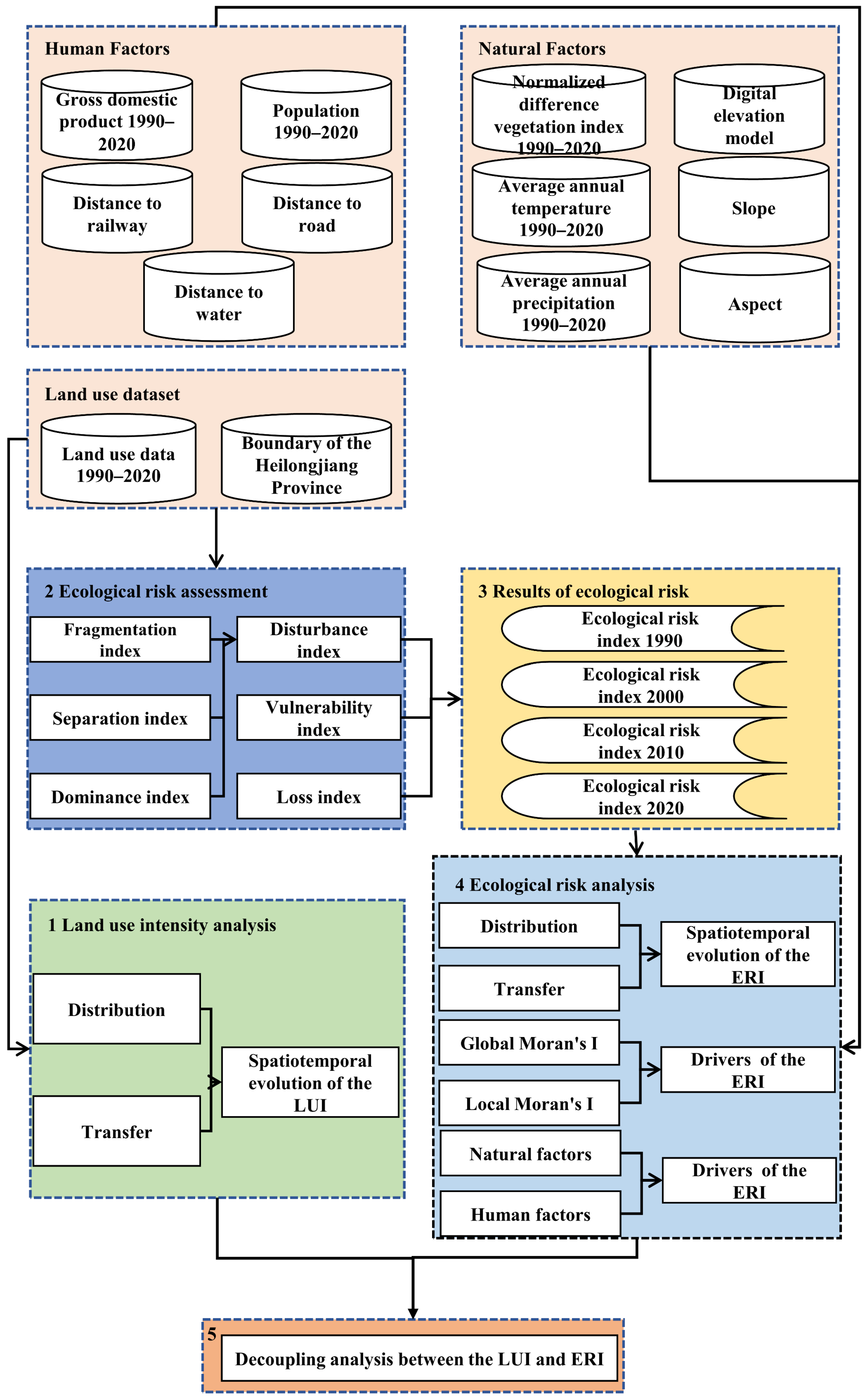
2. Materials and Methods

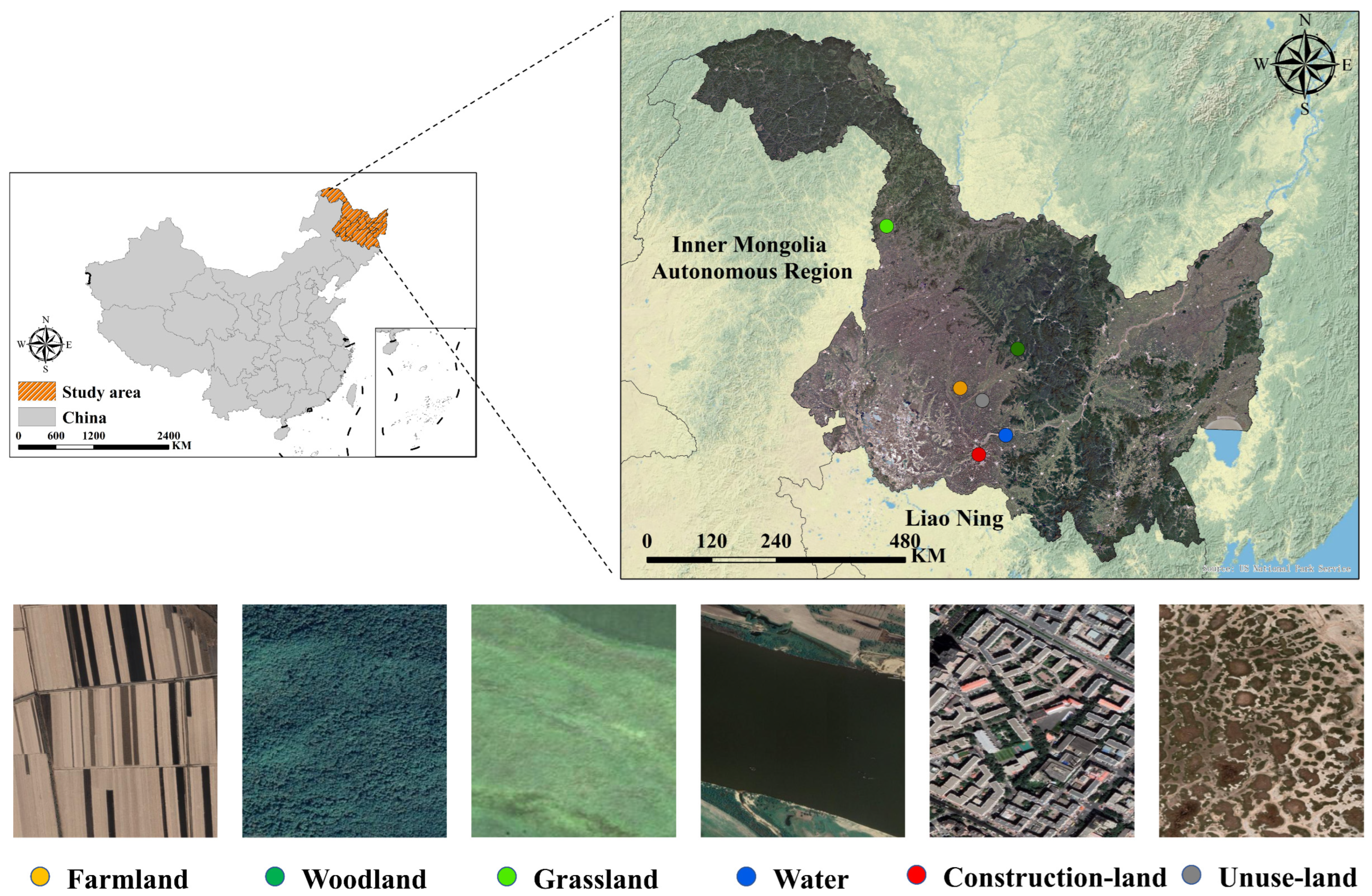
2.1. Study Area

Heilongjiang Province is situated in the northernmost part of China and covers an area of 473,000 km², extending from 121°11′ to 135°05′ east longitude and 43°26′ to 53°33′N latitude (Figure 1). The high terrain of the province is located in the northwest and southeast regions, while the northeast and southwest regions are characterized by lower elevations. The annual average temperature in Heilongjiang Province is approximately 2.6 °C, with annual average precipitation of approximately 600 mm [39]. However, rapid urbanization driven by national economic growth and social development has led to excessive land exploitation and utilization, bringing about numerous ecological and environmental challenges [40].

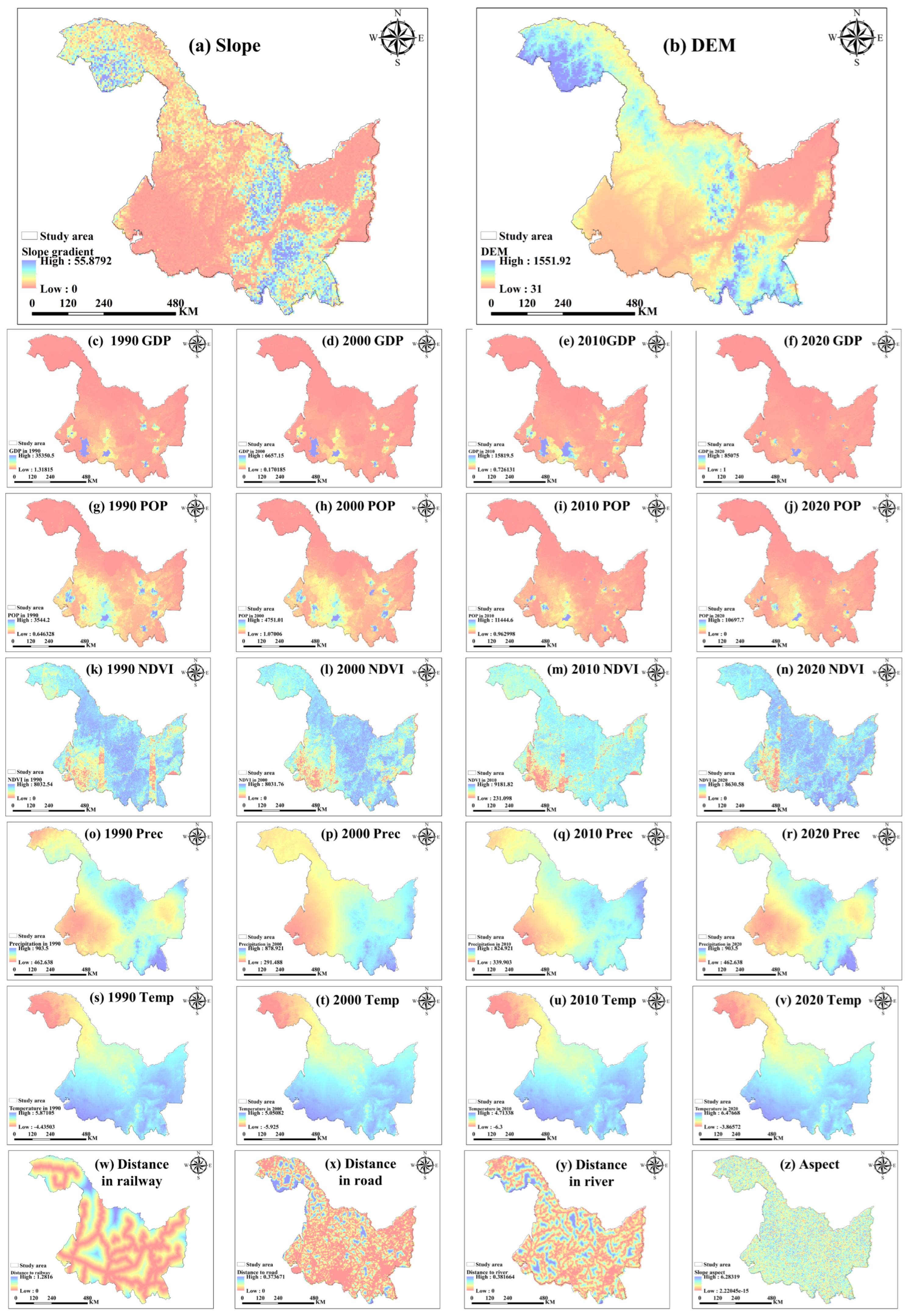
2.2. Data Sources and Processing

The study utilized a variety of data sources, which encompassed land use data, annual average temperature, annual total precipitation, normalized difference vegetation index (NDVI), gross domestic product (GDP), population density (POP), distance to railway, distance to road, distance to riverbank, the DEM, and slope gradient and slope aspect data (

Table 1. Dataset details and sources.

Type	Name	Content	Resolution	Source	Year
Land use cover data	National Land-use/Cover Database of China	Farmland, woodland, grassland, water, construction land, unused land	30 m	RESDC (https://www.resdc.cn/) (accessed on 1 July 2024)	1990/2000/2010/2020
Geographic Big Data	GDP Distribution	Total GDP within 1 km2	1 km	RESDC (https://www.resdc.cn/) (accessed on 1 July 2024)	1995/2000/2010/2020
	Population Distribution	Average environmental population value	1 km	RESDC (https://www.resdc.cn/) (accessed on 1 July 2024)	1990/2000/2010/2020
	Distance to Railway	/	1 km	Open Street (https://www.openstreetmap.org/) (accessed on 1 July 2024)	/
	Distance to Road	/	1 km	Open Street (https://www.openstreetmap.org/) (accessed on 1 July 2024)	/
	Distance to River	/	1 km	Open Street (https://www.openstreetmap.org/) (accessed on 1 July 2024)	/
Vegetation elements	Normalized Difference Vegetation Index (NDVI)	Annual NDVI maximum dataset	30 m	Google Earth Engine (https://earthengine.google.com/) (accessed on 2 July 2024)	1990/2000/2010/2020
Meteorological elements	Precipitation	Annual total precipitation	1 km	Google Earth Engine (https://earthengine.google.com/) (accessed on 2 July 2024)	1990/2000/2010/2020
	Temperature	Annual average temperature	1 km	Google Earth Engine (https://earthengine.google.com/) (accessed on 2 July 2024)	1990/2000/2010/2020
Terrain elements	Topography	Digital elevation model	1 km	Google Earth Engine (https://earthengine.google.com/) (accessed on 2 July 2024)	/
	Slope Gradient	/	1 km	/	/
	Slope Aspect	/	1 km	/	/

and Figure 2).

The land use data analyzed in this study encompass four distinct periods—the 1990s, 2000s, 2010s, and 2020s—each characterized by a spatial resolution of 30 m. This dataset was sourced from the Data Center of Resources and Environmental Sciences of the China Academy of Sciences (RESDC), and it boasts an accuracy rating of 90%, making it the most precise publicly accessible land use product available. The spatial distribution of the GDP was obtained from the RSEDC, which has a resolution of 1 km. Owing to the lack of the GDP spatial distribution data for 1990, the GDP spatial distribution data for 1995 were used instead. Furthermore, population distribution data (POP) spanning from 1990 to 2020 were also sourced from the RSEDC, maintaining the same 1 km spatial resolution. Both the population and the GDP data, organized according to administrative districts, were allocated onto the spatial grid via a multifactor weight distribution approach.

The railway, road, and river data were retrieved from the OpenStreetMap website. Subsequently, the shortest Euclidean distances to these features were computed utilizing ArcGIS.

The NDVI data from 1990 to 2020 were collected from the Google Earth Engine (GEE) platform, featuring a spatial resolution of 30 m. These data were from the annual maximum NDVI dataset calculated from the Landsat 5/8 remote sensing images.

The annual total precipitation and annual average temperature data from 1990 to 2020 were calculated from the monthly average temperature data and monthly total precipitation data of the EAR5 product in the GEE, with a spatial resolution of 1 km.

The DEM data were collected from the GEE platform, and their spatial resolution was 90 m. This dataset originates from the Space Shuttle Radar Topography Mission (SRTM).

2.3. Method

This study is based on Heilongjiang’s land use data, climate data, and socioeconomic data in 1990, 2000, 2010, and 2020. First, through the land use intensity index and ecological risk index, the spatiotemporal evolution characteristics of land use types, the LUI, and ERI in Heilongjiang Province from 1990 to 2020 are systematically analyzed. Secondly, the main driving factors affecting the ERI are explored, and the OPGD is entered. Finally, the decoupling model is combined to analyze the action mechanism of the LUI and ERI. The specific framework is shown in Figure 3.

2.3.1. Land Use Intensity

LUI is mainly used to reflect the intensity of land use and study the impact of natural and human activity factors on land use development [41]. Its calculation formula is as follows:

$$LUI=100\times {\sum }_{i=1}^n{\displaystyle \frac{S_i}{{\sum }_{i=1}^n{S}_i}}\times D_i$$

(1)

where $LUI$ represents the land use intensity; n is the number of land use types; $S$ is the total area of the research unit (km²); $S_i$ is the area of the $i$ type of land use; and $D_i$ is the $i$ type of land use intensity assignment, based on the past [42,43]. The research results divide different land types into 4 categories and assign different weights, namely, 3 for farmland, 2 for woodland, 2 for grassland, 2 for water, 4 for construction land, and 1 for unused land, respectively.

2.3.2. Ecological Risk Assessment

This research identifies landscape disturbance, landscape fragility, landscape loss, and the ERI as crucial elements influencing the stability of regional ecosystems. A model was developed to evaluate the ERI based on these factors. Furthermore, this study examined the trends in regional landscape ERI linked to changes in land use.

(1) Division of the ERI sampling units

In this study, the average patch area of the landscape type is 2 km × 2 km. Previous studies set the calculation unit to 2–5 times higher than the average patch area. Therefore, this study set nine different scales within the range of 2–5 times higher than the average patch area of landscape types, including 4 km × 4 km, 5 km × 5 km, 6 km × 6 km, 7 km × 7 km, 8 km × 8 km, 9 km × 9 km, 10 km × 10 km, 11 km × 11 km, and 12 km × 12 km, which were used to identify the most suitable scale for assessing the ERI in Heilongjiang Province. The results of the ERI calculations at each scale were then subjected to spatial autocorrelation analysis to determine the optimal scale. The spatial distribution data for the ERI in Heilongjiang Province were subsequently obtained via the Kriging interpolation method [44].

(2) Landscape disturbance index

The landscape disturbance index (LDI) serves as a measure of the intensity of ex-ternal disruptions across various landscape types, in which an increase in disturbance correlates with a heightened ERI. The LDI comprises three primary components: landscape fragmentation, landscape separation, and landscape dominance [45,46]. The formula is as follows:

$${LDI}_i={aC}_i+{bF}_i+{cD}_i$$

(2)

$C_i$ is the landscape fragmentation index:

$$C_i={\displaystyle \frac{N_i}{A_i}}$$

(3)

$F_i$ is the landscape separation index:

$$F_i={\displaystyle \frac{A}{{2A}_i}}\sqrt{{\displaystyle \frac{N_i}{A_i}}}$$

(4)

$D_i$ is the landscape dominance index:

$$D_i={\displaystyle \frac{M_i+L_i}{2}};M_i={\displaystyle \frac{N_i}{N}};L_i={\displaystyle \frac{A_i}{A}}$$

(5)

The weights assigned to the indices, represented by $a$, $b$, and $c$, reflect the relative importance assigned to each index. Importantly, the sum of these weights should equal 1. $N_i$ signifies the number of patches corresponding to landscape type $i$, while $N$ represents the overall total number of patches. $A_i$ denotes the total area covered by landscape type $i$. $A$ indicates the total area of the landscape. $M_i$ refers to the relative density of the landscape type. $L_i$ represents the relative coverage of the landscape type. On the basis of relevant references, expert opinions, and literature assessments, weights of 0.5, 0.3, and 0.2 were assigned to these three indicators [47].

(3) Landscape vulnerability index

The landscape vulnerability index (LVI) serves as a measure of an ecosystem’s sensitivity to external factors. A higher index value suggests a greater level of ecosystem instability. Since 2000, unused land has been widely accepted as the most vulnerable area, with its LVI being assigned a value of 6 [48,49,50,51]. Water, farmland, woodland, and grassland were assigned values of 5, 4, 3, and 2, respectively. The possibility of transforming construction land into other landscape types was considered the lowest and was thus assigned a value of 1.

(4) Landscape loss index

The landscape loss index (LLI) quantifies the extent of loss that different types of landscapes endure when subjected to external pressures. The LLI consists of two key components: the landscape interference index and the landscape vulnerability index. The equation is expressed as follows:

$${LLI}_i={LVI}_i+{LDI}_i$$

(6)

where ${LVI}_i$ is the landscape vulnerability index of landscape type $i$, and ${LDI}_i$ is the landscape vulnerability index of landscape type $i$.

(5) Landscape ecological risk index

The ERI is derived from the indices mentioned earlier and incorporates multiple factors. An elevated ERI indicates a higher level of risk. The formula for calculating the ERI is as follows:

$${ERI}_i={\sum }_{i=1}^n{\displaystyle \frac{A_i}{A}}{LLI}_i$$

(7)

where $A_i$ represents the total area corresponding to landscape type i, $A$ denotes the aggregate landscape area, and ${LLI}_i$ signifies the landscape loss index specific to landscape type $i$.

In accordance with previous studies [52,53], this study categorizes the ERI into five distinct levels by employing the natural break-point technique. These levels are as follows: low ecological risk area (ERI ≤ 0.0711), relatively low ecological risk area (0.0711 < ERI ≤ 0.1504), moderate ecological risk area (0.1504 < ERI ≤ 0.2882), relatively high ecological risk area (0.2882 < ERI ≤ 0.5637), and high ecological risk area (ERI > 0.5637).

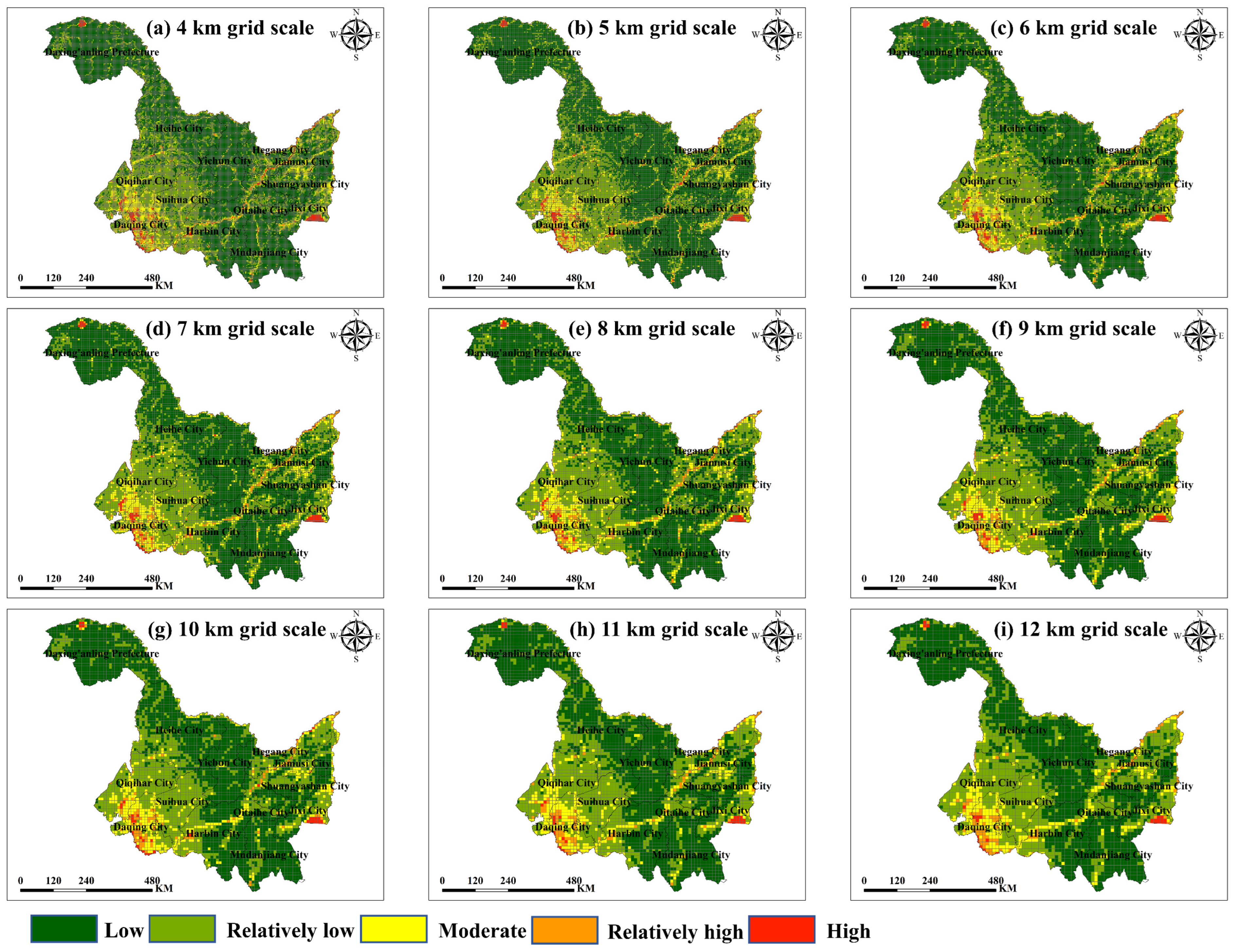
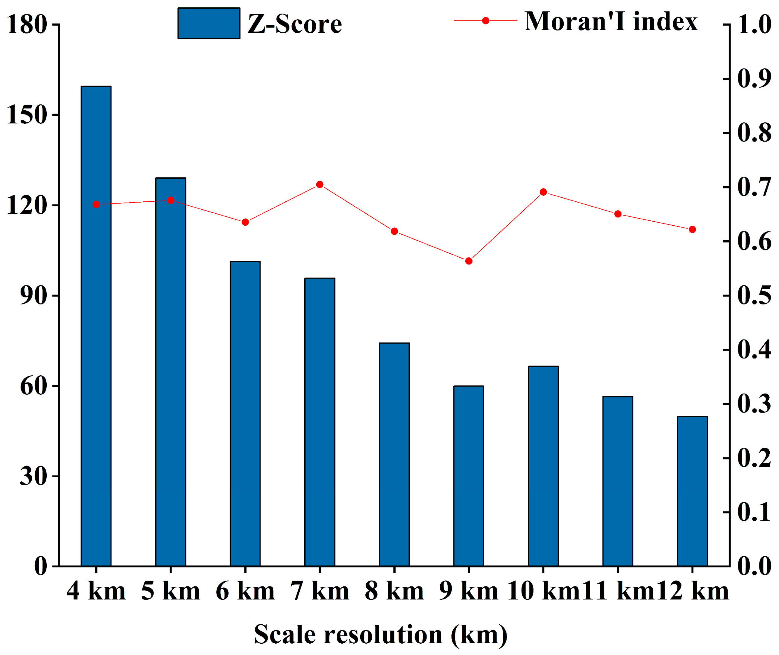
2.3.3. Spatial Autocorrelation

Moran’s I index and the LISA index were used to assess the spatial autocorrelation of ecological risk in Heilongjiang Province. Moran’s I index is used to determine whether there is spatial autocorrelation between adjacent units of the ERI. The calculation formula is as follows:

$$I={\displaystyle \frac{n{\sum }_i{\sum }_j\omega (Y_i-\overline{Y})(Y_j-\overline{Y})}{\left({\sum }_{i\ne j}{\omega }_{ij}\right){\sum }_i{(Y_i-\overline{Y})}^2}}$$

(8)

$Y_i$ and $Y_j$ are the ERI values of adjacent sampling units. ${\omega }_{ij}$ is the spatial weight matrix. $\overline{Y}$ is the average value of the ERI. An I value greater than 0 indicates strong spatial aggregation and positive spatial correlation. An I value less than 0 indicates strong spatial dispersion and negative spatial correlation. When the value I is equal to 0, there is no spatial correlation.

The LISA index is a spatial autocorrelation measure commonly employed to analyze the similarity between adjacent areas within a given region. It determines the level of spatial autocorrelation by calculating the correlation between each geographical unit and its neighboring units in geospatial data. The calculation formula is as follows:

$$I_i={\displaystyle \frac{Y_i-\overline{Y}}{S^2}}{\sum }_{j\ne i}^{n^{\prime }}{\omega }_{ij}(Y_j-\overline{Y})$$

(9)

$$S^2={\displaystyle \frac{1}{n^{\prime }}}\sum {(Y_i-\overline{Y})}^2$$

(10)

$n^{\prime }$ is the number of sampling units. $S^2$ is the variance of the sampling unit. A value of $I_i$ greater than 0 indicates that an area with a high ERI value is surrounded by an area with a high ERI value, or an area with a low ERI value is surrounded by an area with a low ERI value, showing “high-high” or “low-low” aggregation. A value of $I_i$ less than 0 indicates that an area with a high ERI value is surrounded by an area with a low ERI value, or an area with a low ERI value is surrounded by an area with a high ERI value, showing “high-low” or “low-high” aggregation. When the value of $I_i$ is equal to 0, this area has no correlation with its neighboring areas.

2.3.4. The Optimal Parameter-Based Geographical Detector (OPGD) Model

Geographic detector is a statistical tool designed to explore the spatial variation in data and its influencing factors. These detectors are divided into four main types: factor detection, interaction detection, risk area detection, and ecological detection. This study employed a factor detector to evaluate how various factors contribute to the spatial variation in the ERI, with the q value indicating the strength of each factor’s influence. A higher q value denotes a more significant explanatory power of the factor regarding the ERI. This study utilized the OPGD to examine the driving factors behind the ERI. The model incorporates several classification methods, including equal interval classification, natural break classification, quantile classification, and standard deviation classification, to identify parameters with the highest q values for geographic detector analysis. The q value, representing the explanatory power of a factor, was calculated as follows:

$$q=1-{\displaystyle \frac{1}{{N\sigma }^2}}{\sum }_{j=1}^{\mathrm{L}}{N}_j{\sigma }_j^2$$

(11)

where $N_j$ and $N$ denote the number of units in area j and the total number of units in the study area, respectively; ${\sigma }_j^2$ and ${\sigma }^2$ represent the variances within area j and across the entire study area, respectively; and L signifies the number of partitions. The q value ranges between 0 and 1, with higher values indicating a stronger influence of the factor on the regional differentiation of the ERI.

Interactive detection is employed to assess whether the combined influence of two factors provides a more robust explanation for the ERI. The interaction detector builds the factor detection approach by evaluating the relative significance of two interacting factors. The interaction effect is analyzed by comparing the outcomes of individual factor analyses with those obtained when both factors are considered simultaneously. The interaction types of factor detectors include the following five types (

Table 2. Factor interaction categories.

Interaction Type	Judgment Basis
Non-linear weakening	$q ({\mathrm{X}}_1\cap {\mathrm{X}}_2)<\mathrm{M}\mathrm{i}\mathrm{n}(q ({\mathrm{X}}_1),q ({\mathrm{X}}_2\left)\right)$
Single-factor non-linear attenuation	$\mathrm{M}\mathrm{i}\mathrm{n}\left(q \left({\mathrm{X}}_1\right),q \left({\mathrm{X}}_2\right)\right)<q ({\mathrm{X}}_1\cap {\mathrm{X}}_2)<\mathrm{M}\mathrm{a}\mathrm{x}(q ({\mathrm{X}}_1),q({\mathrm{X}}_2\left)\right)$
Two-factor interaction enhancement	$q ({\mathrm{X}}_1\cap {\mathrm{X}}_2)>\mathrm{M}\mathrm{a}\mathrm{x}(q ({\mathrm{X}}_1),q ({\mathrm{X}}_2\left)\right)$
Non-linear enhancement	$q \left({\mathrm{X}}_1\cap {\mathrm{X}}_2\right)=q \left({\mathrm{X}}_1\right)+q \left({\mathrm{X}}_2\right)$
Mutual independence	$q \left({\mathrm{X}}_1\cap {\mathrm{X}}_2\right)>q \left({\mathrm{X}}_1\right)+q \left({\mathrm{X}}_2\right)$

).

2.3.5. Decoupling Analysis Model

In order to study the synergistic effect between the LUI and ERI, a decoupling analysis model of land use and the ERI in Heilongjiang Province was constructed through the decoupling elasticity index [54,55]. The calculation formula is as follows:

$$D_t={\displaystyle \frac{∆ERI}{∆LUI}}={\displaystyle \frac{({ERI}_c-{ERI}_s)/{ERI}_s}{{(LUI}_c-{LUI}_s)/{LUI}_s}}$$

(12)

$D_t$ is the decoupling elasticity coefficient of the t period; ${ERI}_c$ and ${ERI}_s$ are the ERI of the base year and the last year of the t period, respectively; $∆ERI$ is the rate of change of the ERI in the t period; ${LUI}_c$ and ${LUI}_s$ are the LUI of the base year and the last year; $∆LUI$ is the rate of change of the LUI in the t period. Based on the past [56,57,58,59], the eight decoupling states defined by the decoupling analysis are shown in

Table 3. Decoupling state types and their decisive intervals.

Decoupling Type	Decisive Interval	Interpretation
Expansive negative decoupling (ENDC)	$∆LUI>0, ∆ERI>0,D>1.2$	ERI increases with LUI, and its growth rate is greater than that of LUI.
Expansive coupling (EC)	$∆LUI>0, ∆ERI>0, 0.8\le D\le 1.2$	ERI increases with LUI at the same rate
Weak decoupling (WDC)	$∆LUI>0, ∆ERI>0, 0<D<0.8$	ERI and LUI increase simultaneously, but the growth rate of ERI is lower than that of LUI
Strong decoupling (SDC)	$∆LUI<0, ∆ERI>0,D<0$	ERI decreases with increasing LUI
Recessive decoupling (RDC)	$∆LUI<0, ∆ERI<0,D>1.2$	ERI and LUI decreased simultaneously, but the reduction in ERI was greater than that in LUI
Recessive coupling (RC)	$∆LUI<0, ∆ERI<0, 0.8\le D\le 1.2$	ERI decreases with LUI at the same rate
Weak negative decoupling (WNDC)	$∆LUI<0, ∆ERI<0, 0<D<0.8$	ERI and LUI are reduced at the same time, but the reduction in ERI is smaller
Strong negative decoupling (SNDC)	$∆LUI>0, ∆ERI<0,D<0$	ERI increases as LUI decreases

.

3. Results

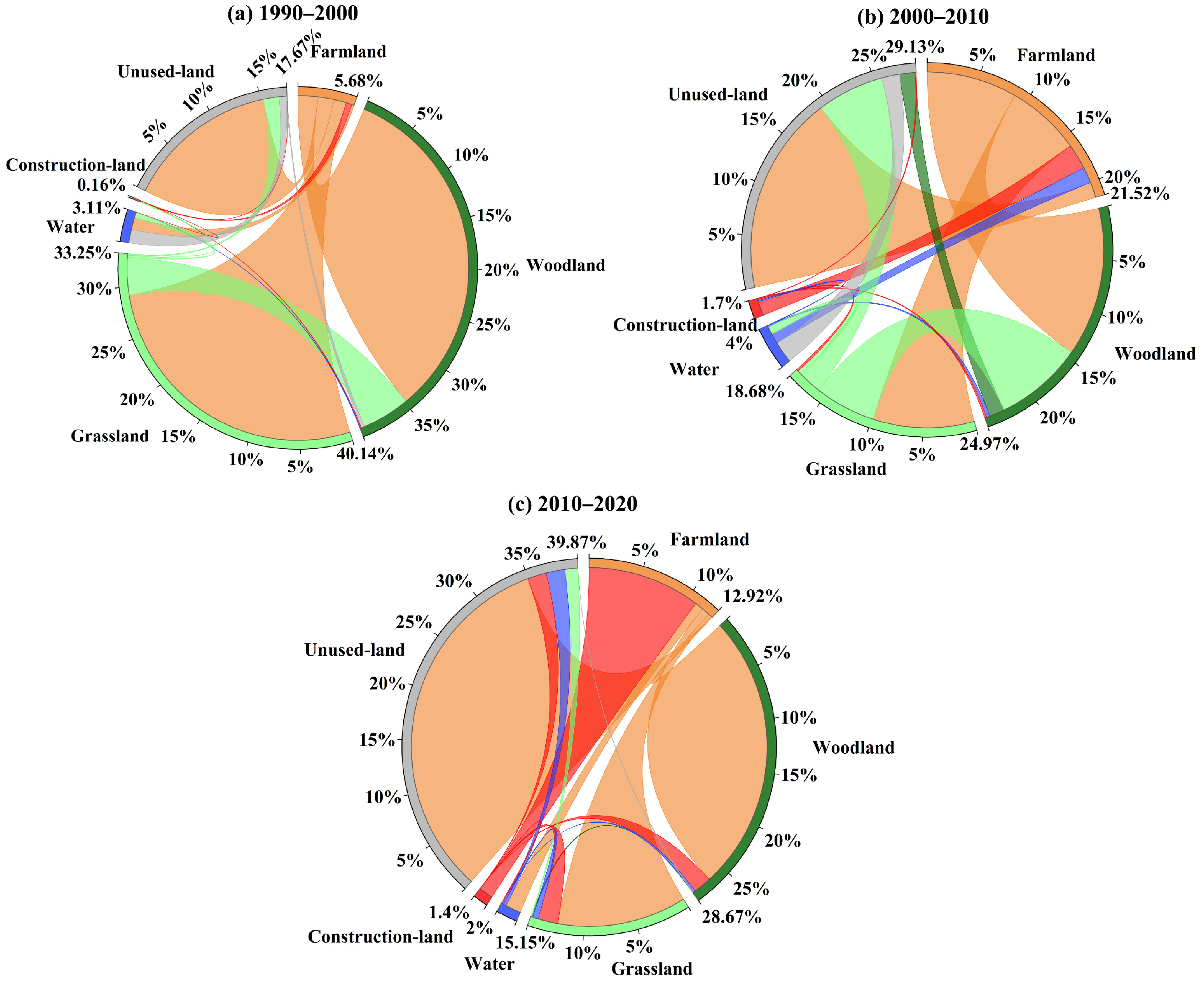
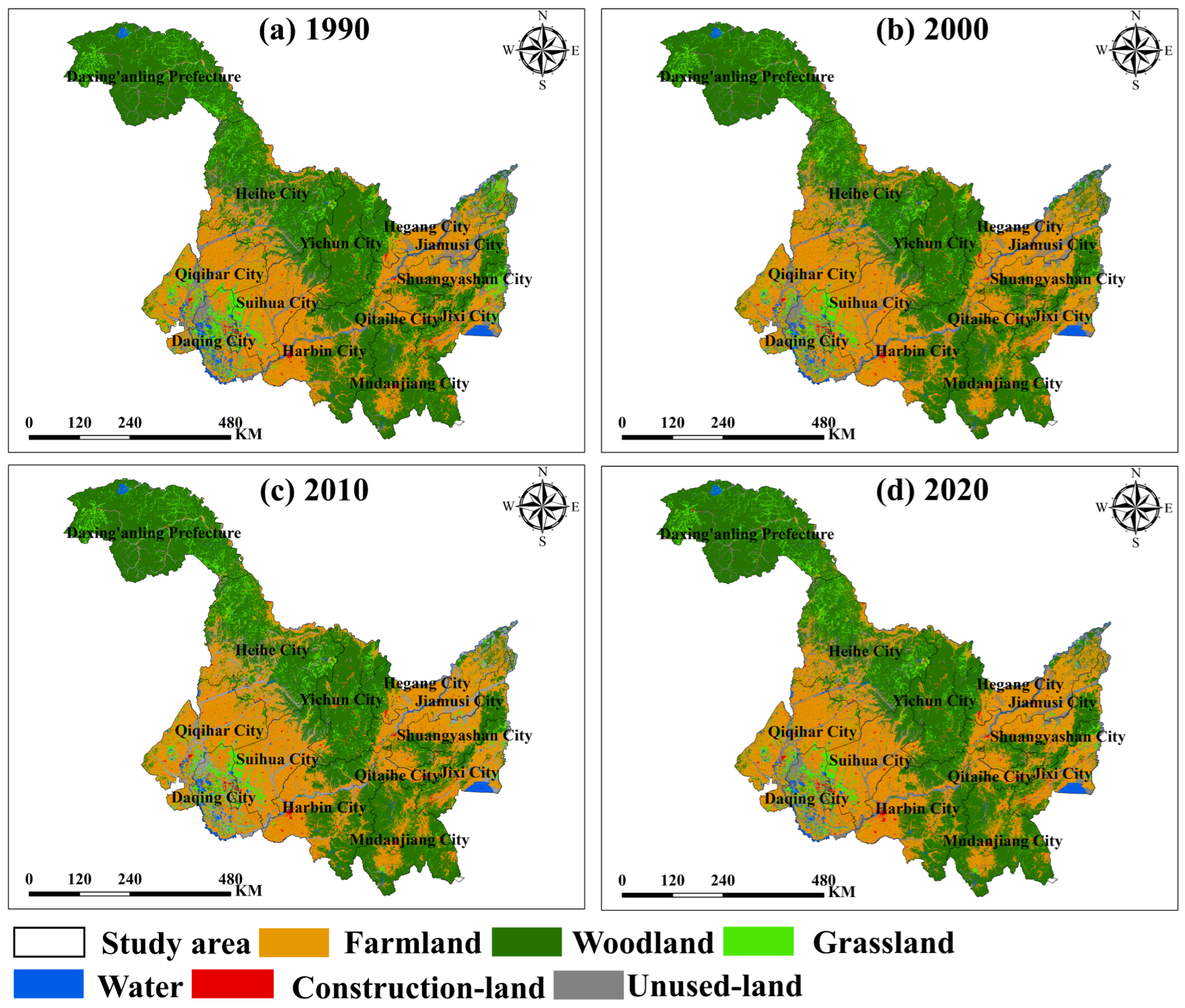
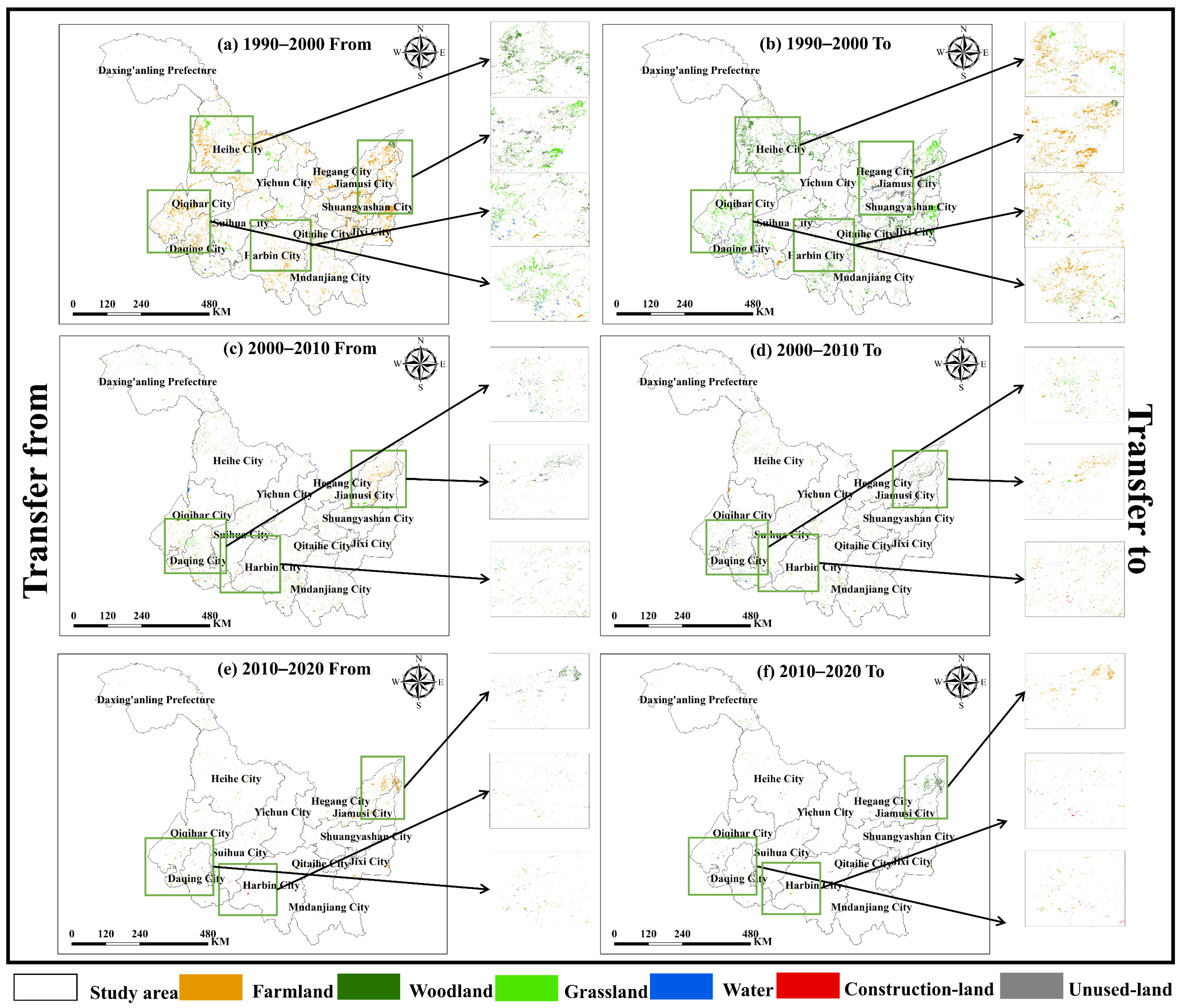
3.1. Spatiotemporal Changes in Land Use Types in Heilongjiang Province

Table 4. Area and proportion of land use types in Heilongjiang Province from 1990 to 2020.

Land Use Type	1990		2000		2010		2020
	Area (km2)	Proportion (%)	Area (km2)	Proportion (%)	Area (km2)	Proportion (%)	Area (km2)	Proportion (%)
Farmland	141,709	31.31	159,765	35.30	161,432	35.67	163,353	36.10
Woodland	212,118	46.87	203,841	45.04	203,260	44.91	202,425	44.73
Grassland	38,568	8.52	32,533	7.19	32,838	7.26	32,437	7.17
Water	9961	2.20	9510	2.10	9526	2.10	9569	2.11
Construction land	8842	1.95	8976	1.98	9066	2.00	9517	2.10
Unused land	41,360	9.14	37,933	8.38	36,437	8.05	35,257	7.79

presents the land use types in Heilongjiang Province from 1990 to 2020, as well as their areas and proportions. The data revealed that woodland and farmland were the dominant land use types, accounting for more than 75% of the total area. Over the past 30 years, significant changes have occurred in the land use patterns of Heilongjiang Province. While construction land and farmland consistently expanded, other land use types generally decreased, particularly woodland and unused land. The area of farmland experienced a notable increase of 18,056 km² between 1990 and 2000. Furthermore, grassland exhibited significant volatility, with an overall decline, although it experienced a slight growth of 0.07% from 2000 to 2010. Conversely, the area of water remained relatively stable.

Figure 4 displays the land use transfer matrix in Heilongjiang Province from 1990 to 2020. During the period from 1990 to 2000, the land use change area was 24,116 km². Woodland, grassland, and unused land underwent significant conversion into farmland, accounting for 8401 km², 7037 km², and 3683 km², respectively. These conversions represented 35%, 29%, and 15% of the total land conversion area, respectively. Additionally, mutual transformations between woodland and grassland occurred, with 1162 km² of woodland converted into grassland (5%) and 895 km² of grassland converted into woodland (4%). The increase in construction land primarily originated from farmland, with 141 km² of farmland being transformed. Between 2000 and 2010, the land use change area in Heilongjiang Province was 6846 km². Woodland, grassland, and unused land were converted into farmland, accounting for 985 km², 675 km², and 1318 km², respectively. These conversions represented 43% of the total land conversion area. Additionally, unused land and woodland were converted into grassland, with areas of 447 km² and 586 km², respectively, accounting for 16% of the total land circulation area. Moreover, 168 km² of farmland was transformed into construction land. From 2010 to 2020, the land use change area was 2999 km², in which woodland, grassland, and unused land were predominantly converted into farmland, accounting for 799 km², 375 km², and 1048 km², respectively, representing 74% of the total land conversion area. Furthermore, 326 km² of farmland was converted into construction land, accounting for 11% of the total land circulation area.

In summary, over the past 30 years, Heilongjiang Province has experienced a significant expansion of farmland and a marked decrease in woodland, while the urbanization process has accelerated, which has had a great impact on the ecological environment.

The spatial changes in land use in Heilongjiang Province from 1990 to 2020 are depicted in Figure 5 and Figure 6. Farmland was concentrated in the southwest and southeast regions of Heilongjiang Province, including Qiqihar, Suihua, Harbin, Hegang, Jiamusi, Shuangyashan, and Jixi. Woodland was mainly distributed in the northwest and southeast parts, including the Daxing’anling Prefecture, Heihe, Yichun, Mudanjiang, and Harbin. Grassland was predominantly found in Suihua, Daqing, and Qiqihar in the southwest of Heilongjiang Province, as well as Jiamusi and Jixi in the northeast. Water was mainly located in Daqing and Jixi. Construction land was distributed in proximity to the cities. Unused land was concentrated in Qiqihar, Daqing, and Jiamusi. Daqing and Qiqihar in the southwest of Heilongjiang Province have relatively complex land use.

During the period from 1990 to 2000, the conversion of woodland to farmland was primarily concentrated in Heihe and Yichun in the north of Heilongjiang Province. Grassland was mainly converted to farmland in Qiqihar and Jiamusi in the southwest and Jixi in the northeast regions of the province. The areas where unused land was transformed into farmland were predominantly Hegang, Jiamusi, and Shuangyashan in the northeast. The conversion of woodland to grassland was primarily observed in Heihe. In addition, grassland was converted to woodland in Jiamusi in the northeast, while unused land was mainly transformed into grassland in Suihua in the central part.

The most significant land use change from 2000 to 2010 occurred in Daqing and Jiamusi, where the conversion was mainly from woodland to farmland in Jiamusi and from unused land and grassland to farmland in Daqing. The transformation from farmland to construction land predominantly occurred in Harbin. From 2010 to 2020, major land use changes were observed in Daqing, Harbin, and Jiamusi, with the conversion mainly from woodland to farmland in Jiamusi, from unused land and grassland to farmland in Daqing, and from farmland to construction land in Harbin.

3.2. Spatiotemporal Variations in the LUI over the Past 30 Years in Heilongjiang Province

The average values of LUI in Heilongjiang Province in the 1990s, 2000s, 2010s, and 2020s were 226.08, 230.89, 231.63, and 232.51, respectively. The LUI exhibited the most significant increase from 1990 to 2000. Compared with the 1990s, the LUI in the 2020s increased by 2.84%. Apart from a 2.13% increase from 1990 to 2000, the LUI remained relatively stable from 2000 to 2020. This stability can be attributed to policies such as the conversion of farmlands to woodlands and grasslands, implemented after 2000, which contributed to ecological restoration, reduced the LUI of farmland, and consequently mitigated the growth of the LUI.

The spatial distribution of the LUI in Heilongjiang Province exhibits higher values in the southwest and northeast, while lower values are observed in the northwest and southeast (Figure 7 and Figure 8). From 1990 to 2000, except for Daxing’anling Prefecture, all other prefectures and cities experienced an upward trend in the LUI. Between 2000 and 2010, decreases in the LUI were primarily observed in Harbin, Jiamusi, Mudanjiang, and Qitaihe, whereas increases were concentrated in Qiqihar, Daqing, and Jiamusi. From 2010 to 2020, the areas where the LUI increased were primarily located in Hegang, Jiamusi, Qiqihar, and Daqing.

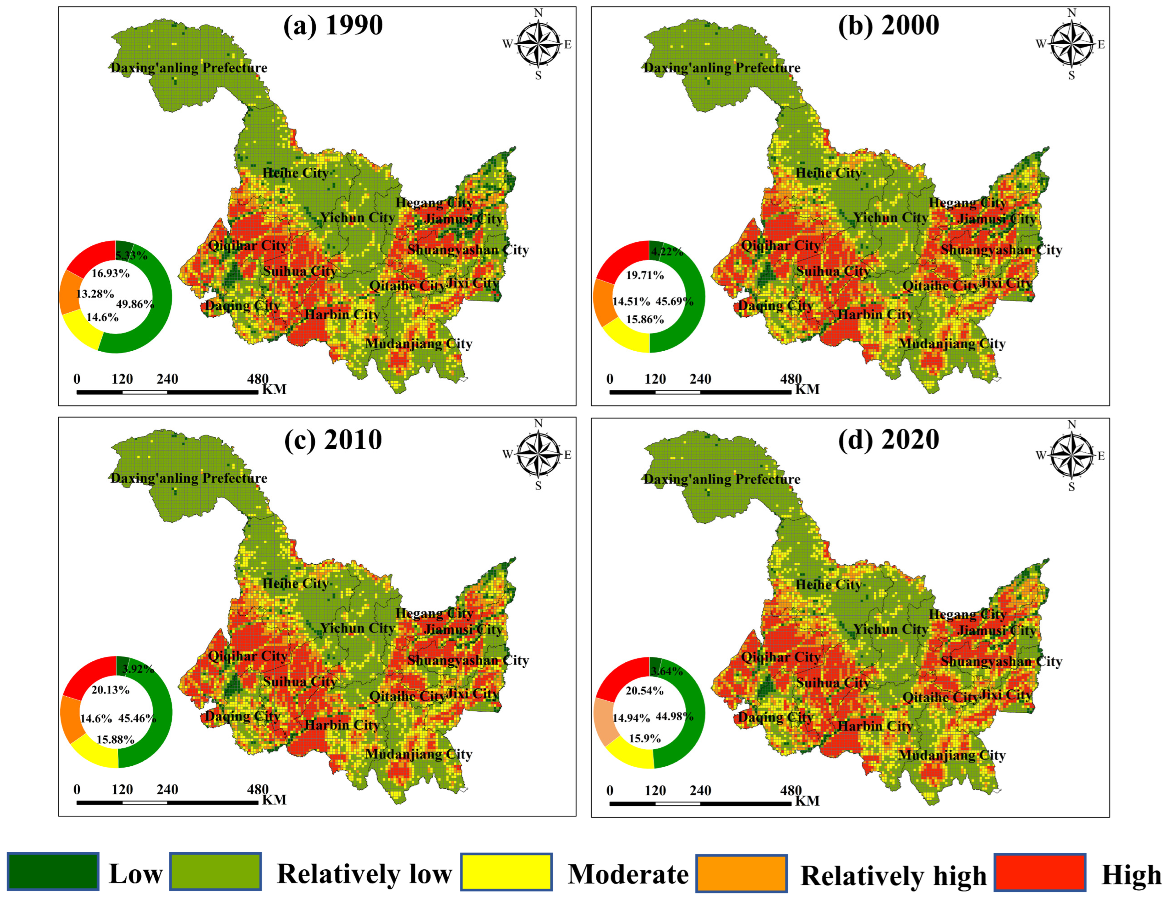
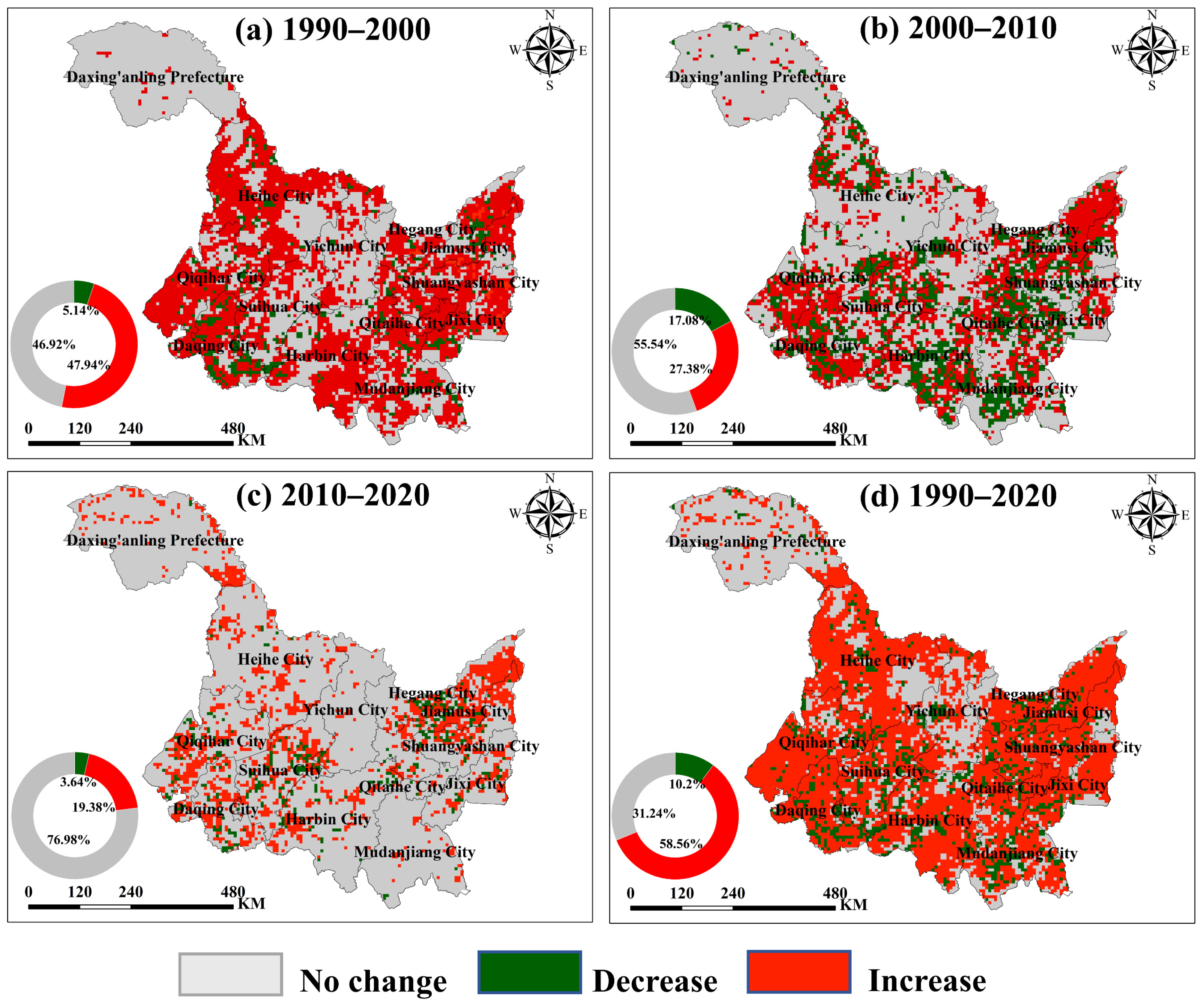
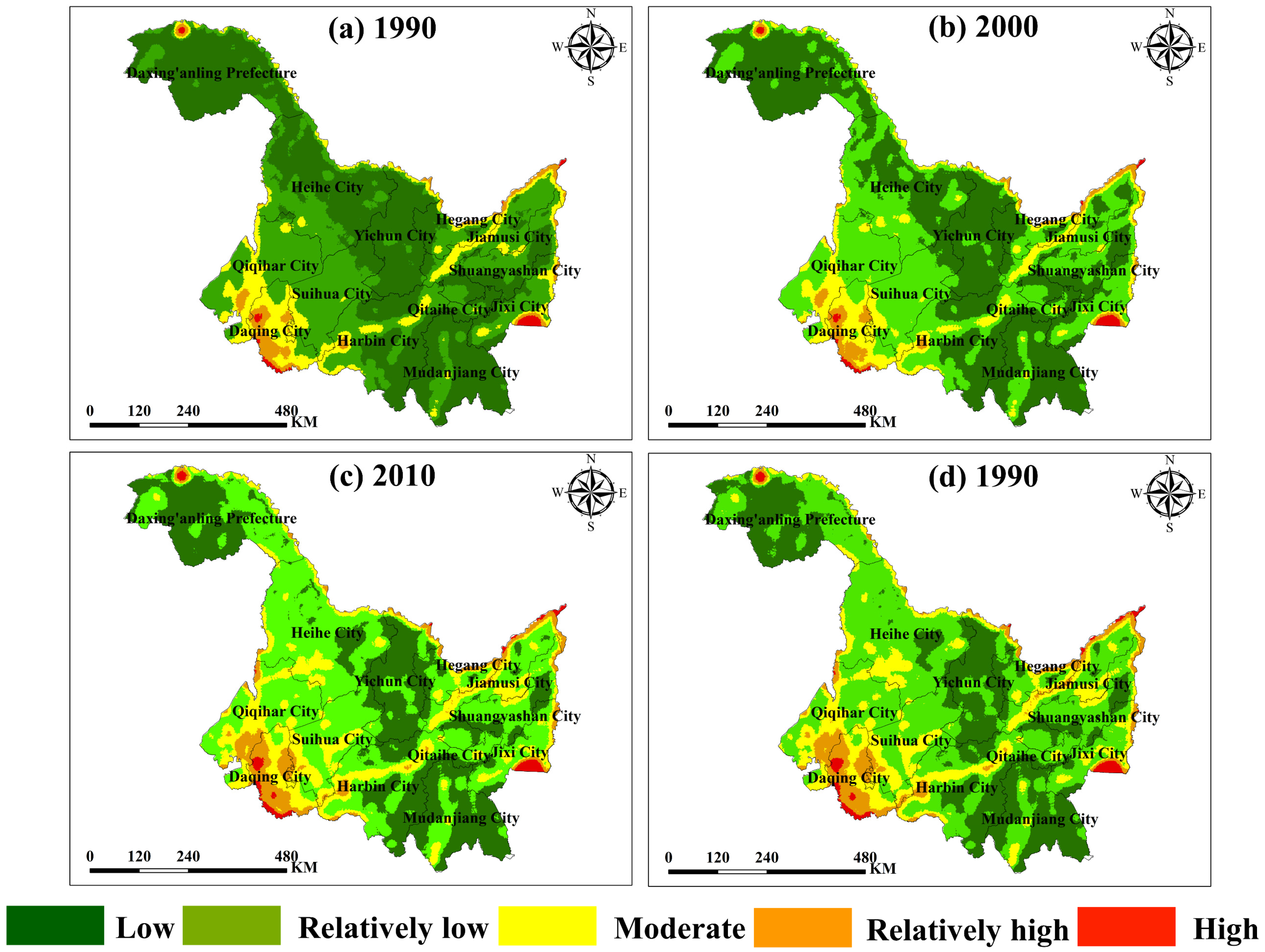
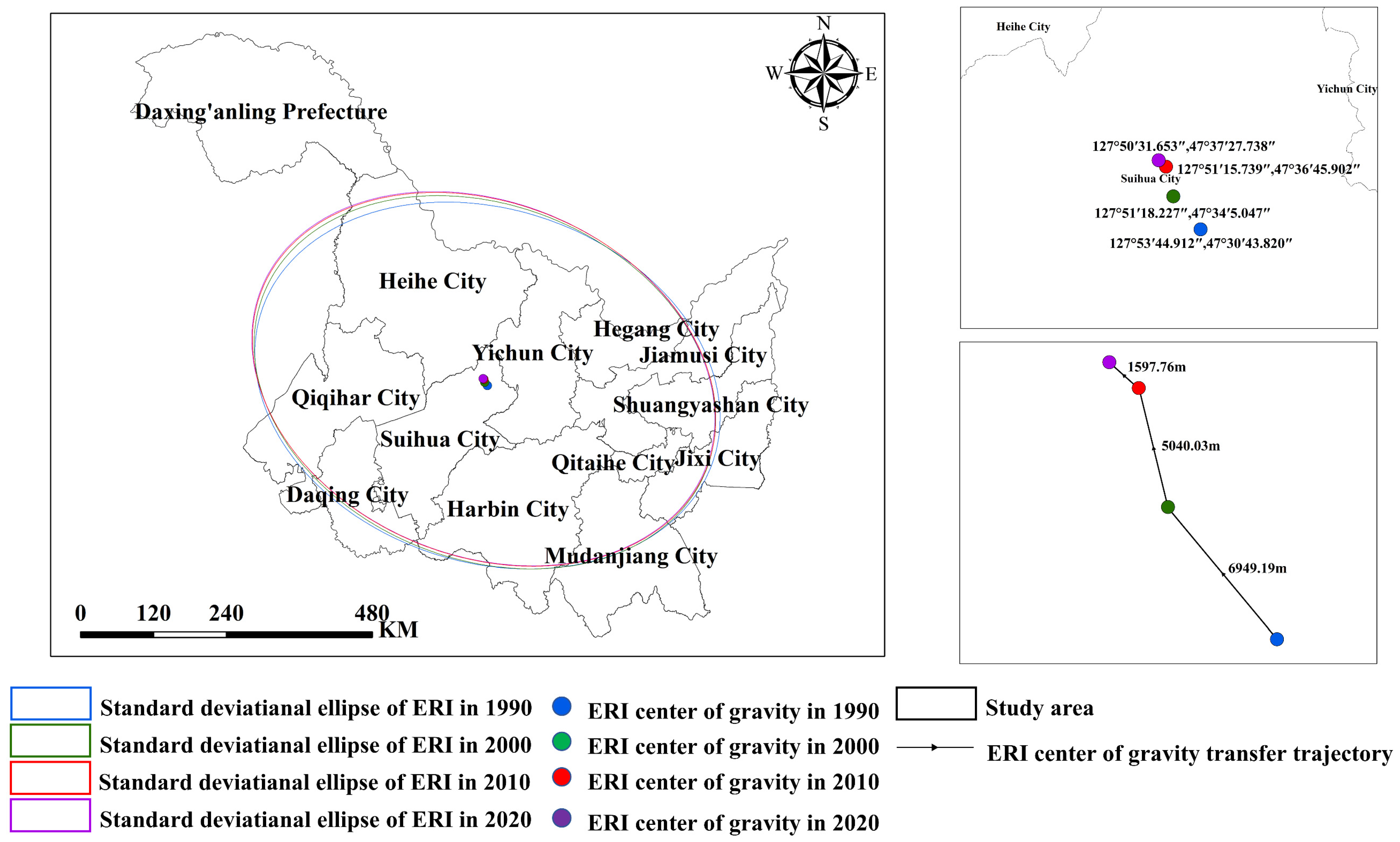
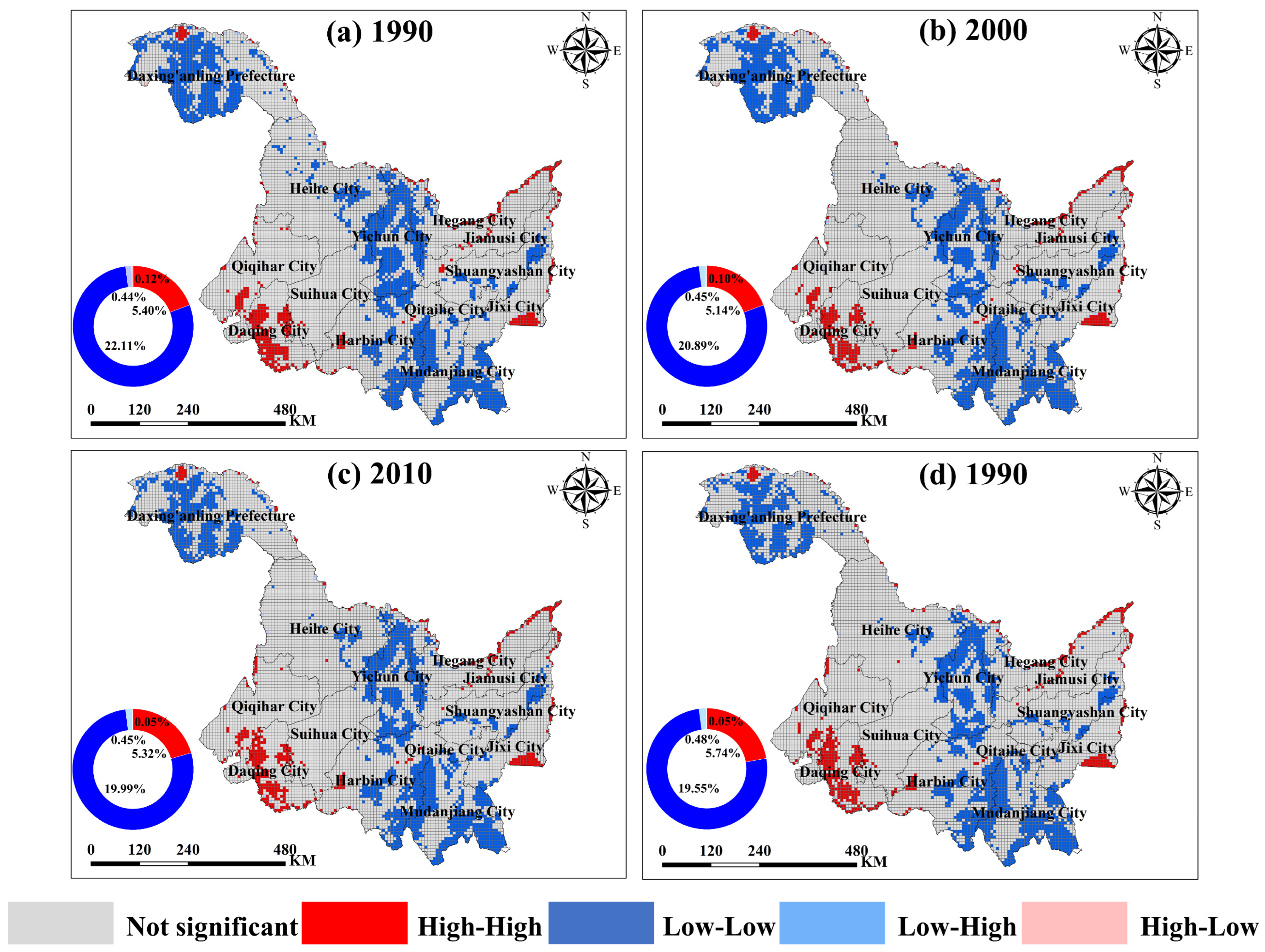
3.3. Spatiotemporal Patterns of the ERI in Heilongjiang Province

To determine the optimal scale for assessing the ERI in Heilongjiang Province, this study considered nine different grid sizes: 4 km × 4 km, 5 km × 5 km, 6 km × 6 km, 7 km × 7 km, 8 km × 8 km, 9 km × 9 km, 10 km × 10 km, 11 km × 11 km, and 12 km × 12 km, which ranged from two to five times the average patch area of the landscape type. The Moran’s I index was computed using a global spatial autocorrelation analysis for each scale. The results indicated that the spatial representation of the ERI varied across scales (Figure 9), with smaller grid sizes yielding more precise ERI estimations. The spatial representation of the ERI was strongly dependent on the grid unit size. Furthermore, Figure 10 illustrates the changes in the Moran’s I index across different scales in Heilongjiang Province. The Moran’s I index values for all nine scales were positive, with Z-scores exceeding 2.58 and p-values below 0.01, confirming a 99% confidence level in the spatial clustering of the ERI, thereby rejecting the null hypothesis. The Moran’s I index of the ERI exhibited substantial fluctuations between the 4 km and 12 km scales. However, at the 7 km × 7 km scale, the index peaked at 0.7046, indicating the strongest spatial correlation. Therefore, this study identified 7 km × 7 km as the optimal scale and divided Heilongjiang Province into 9735 computational units for ERI estimation.

The average ERI values for 1990, 2000, 2010, and 2020 were 0.097, 0.099, 0.127, and 0.132, respectively. The average ERI index demonstrated a consistent upward trend, with the most significant increase of 0.028 occurring between 2000 and 2010.

Table 5. Area and proportion of ERI in Heilongjiang Province from 1990 to 2020.

Risk Type	1990		2000		2010		2020
	Area (km2)	Proportion (%)	Area (km2)	Proportion (%)	Area (km2)	Proportion (%)	Area (km2)	Proportion (%)
Low	213,816	47.42	200,931	44.57	135,919	30.15	126,511	28.06
Relatively low	171,096	37.95	183,686	40.74	208,396	46.22	210,563	46.70
Moderate	50,502	11.20	50,574	11.22	77,101	17.10	80,926	17.95
Relatively high	12,826	2.84	12,820	2.84	24,486	5.43	27,502	6.10
High	2614	0.58	2843	0.64	4952	1.10	5352	1.19

presents the variations in ERI levels over this period. Heilongjiang Province was predominantly characterized by low and relatively low risk; however, the low-risk area decreased significantly by 87,305 km², representing a 19.36% reduction in total area proportion. Conversely, areas classified under relatively high-risk levels exhibited an overall expansion. By 2020, the high-risk area had expanded to 5352 km², more than doubling that recorded in 1990 (2614 km²), increasing its proportion from 0.58% to 1.19% of the total area. This trend underscores a continuous degradation of the ecological environment in Heilongjiang Province over the study period.

Figure 11 and Figure 12 illustrate the classification maps of the ERI from 1990 to 2020. Notably, high-risk areas were primarily concentrated in Daqing, located in the southwest, and Jixi, in the southeast. In contrast, moderate-risk zones were mainly distributed across Qiqihar, Daqing, and Harbin in the southwest, as well as Jiamusi in the east. The remaining areas were largely characterized by low and relatively low risk. Between 1990 and 2020, areas where low risk transitioned to relatively low risk were primarily located in Daxing’anling Prefecture, Heihe, Yichun, and Qitaihe. Areas where the relatively low level of risk escalated into moderate risk were concentrated in Heihe, Suihua, Qiqihar, Jiamusi, and Jixi. Additionally, areas where the moderate-risk level increased to the high-risk level were primarily found in Qiqihar and Daqing, while areas where the relatively high level of risk progressed to the high-risk level were primarily located in Daqing and Jixi. Between 1990 and 2000, the ERI changes primarily occurred in Heihe and Jiamusi. Heihe mainly experienced a transition from low risk to relatively low risk, whereas Jiamusi exhibited a shift from relatively low risk to low risk. The period from 2000 to 2010 witnessed the most pronounced the ERI changes in Heilongjiang Province. During this period, areas where the low level of risk transitioned to the relatively low level of risk were primarily located in Daxing’anling Prefecture, Heihe, Hegang, and Qitaihe, while areas where the relatively low level of risk escalated to the moderate level of risk were mainly concentrated in Qiqihar, Suihua, Jiamusi, and Jixi. Areas where the moderate level of risk decreased to the relatively low level of risk were primarily located in Daqing, whereas areas where the relatively high level of risk advanced to the high level of risk were concentrated in Daqing and Jixi. Between 2010 and 2020, the ERI changes were relatively minor and more spatially dispersed. Areas where the low level of risk transitioned to the high level of risk were primarily located in Daxing’anling Prefecture and Heihe, while areas where the relatively low level of risk escalated to the moderate level of risk were mainly distributed in Heihe, Jixi, and Suihua.

The trajectory map (Figure 13) represented the ERI center of gravity from 1990 to 2020. It was evident that the northeastern region of Suihua consistently housed the ERI center of gravity, with a predominant northwestward movement. The most substantial shift occurred from 1990 to 2000, covering a distance of 6949.19 m. Subsequently, from 2000 to 2010, the movement was 5040.03 m, followed by a shorter distance of 1597.76 m from 2010 to 2020. This pattern was primarily attributed to the concentration of ecological deterioration in the northwest of Heilongjiang Province. During this period, numerous low-risk areas transformed into relatively low risk areas, while the medium- and high-risk areas experienced significant growth. The relatively shorter movement distance observed from 2010 to 2020 can be attributed to minimal changes in land use during this period.

The Moran’s I value for the four periods of the 1990s, 2000s, 2010s, and 2020s were 0.705, 0.694, 0.689, and 0.690, respectively (p < 0.001). The spatial distribution exhibited a significant positive correlation and prominent clustering characteristics. The ERI in Heilongjiang Province, as measured by the Moran’s I index, demonstrated a decreasing trend from 1990 to 2010, followed by an increasing trend from 2010 to 2020. This indicated the pattern of the spatial clustering of the ERI in Heilongjiang Province, which was initially decreasing and then subsequently increasing. The area with high–high clustering units was primarily concentrated in Daqing, Qiqihar, and Jixi of the southwest and northeast parts (Figure 14). These regions were mainly composed of grassland, unused land, and water, resulting in these land use types being more susceptible to human activities and exhibiting greater ecological vulnerability. Conversely, the low–low clustering units were distributed in the Daxing’anling Prefecture, Yichun, Mudanjiang, and Harbin of the south and northeast parts. These regions consisted predominantly of woodland with limited human activity, resulting in lower levels of ecological vulnerability and forming a cluster of low-risk areas.

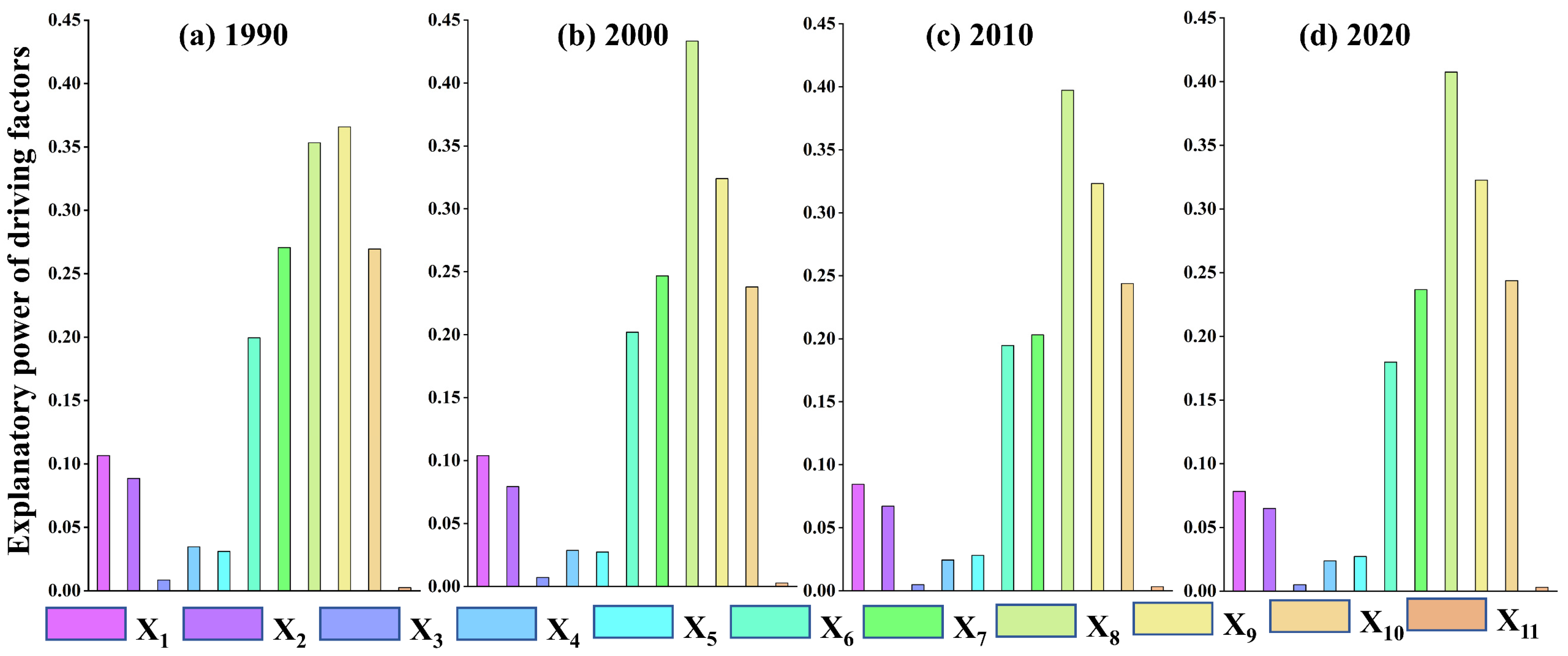
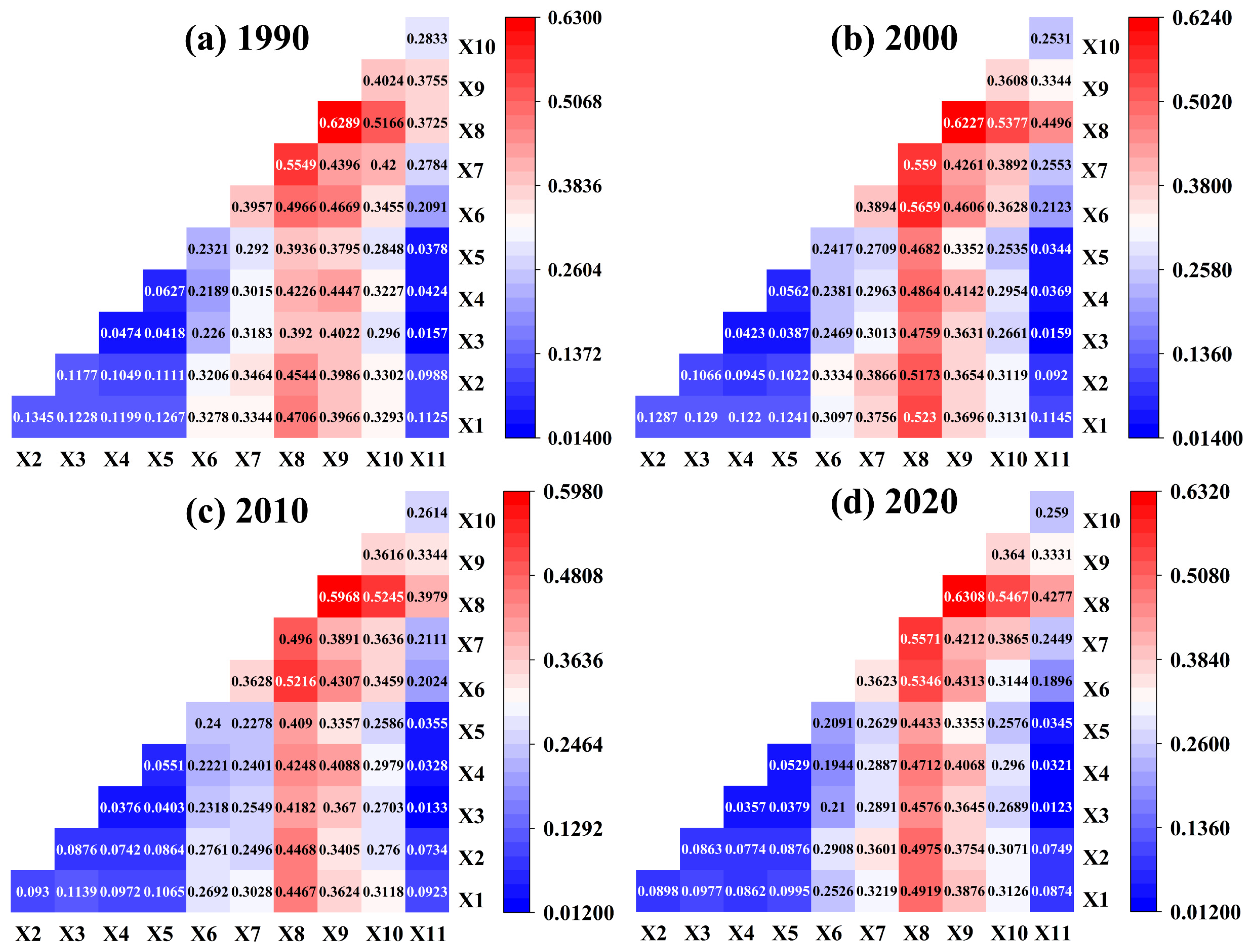
3.4. Impact of Driving Factors on the ERI in Heilongjiang Province

This study employed the OPGD analysis to evaluate the influence of various driving factors on the ERI in Heilongjiang Province. The analysis incorporated both single-factor and multifactor interaction assessments to provide a comprehensive understanding of their impacts.

Figure 15 illustrates the results of the spatial heterogeneity analysis of the ERI using the OPGD. The results indicated that the primary determinants of spatial ERI changes between 1990 and 2020 were the DEM and NDVI, with their explanatory power exceeding 30%. In contrast, the slope aspect exhibited the lowest explanatory capacity, accounting for only approximately 0.3% of the variance. Human factors had a relatively minor influence on the ERI, with the GDP being the most significant, followed by the POP. Other human factors accounted for less than 5% of the variance in the ERI. In 1990, the DEM was the most influential factor affecting the ERI, followed by the NDVI and temperature. By 2000, the NDVI had emerged as the primary determinant of the ERI, followed by the DEM and temperature. In 2010 and 2020, the NDVI and DEM consistently remained the two dominant factors, while the slope aspect emerged as the third most influential factor.

Figure 16 presents the results of the interaction detection analysis regarding the driving factors affecting the ERI. The results indicated that the combined influence of two factors provided greater explanatory power than any single factor alone. This suggested that variations in the ERI in Heilongjiang Province were influenced by the collective impact of multiple driving factors. Between 1990 and 2020, the interaction between the NDVI and other factors consistently demonstrated the highest explanatory power, particularly when combined with the DEM, yielding approximately 60%. Additionally, the interactions between temperature and precipitation with the NDVI were both approximately 50%, highlighting the significant role of natural environmental components, particularly vegetation, in shaping the ERI. The interaction between the DEM and other factors slightly lagged behind that of the NDVI but still exceeded the 30% q value threshold. In contrast, the interaction effects related to human factors were relatively weaker than those associated with natural environmental factors. Among these factors, the coupling of the GDP with other variables had the strongest effect, underscoring the substantial influence of the GDP on the ERI among human factors.

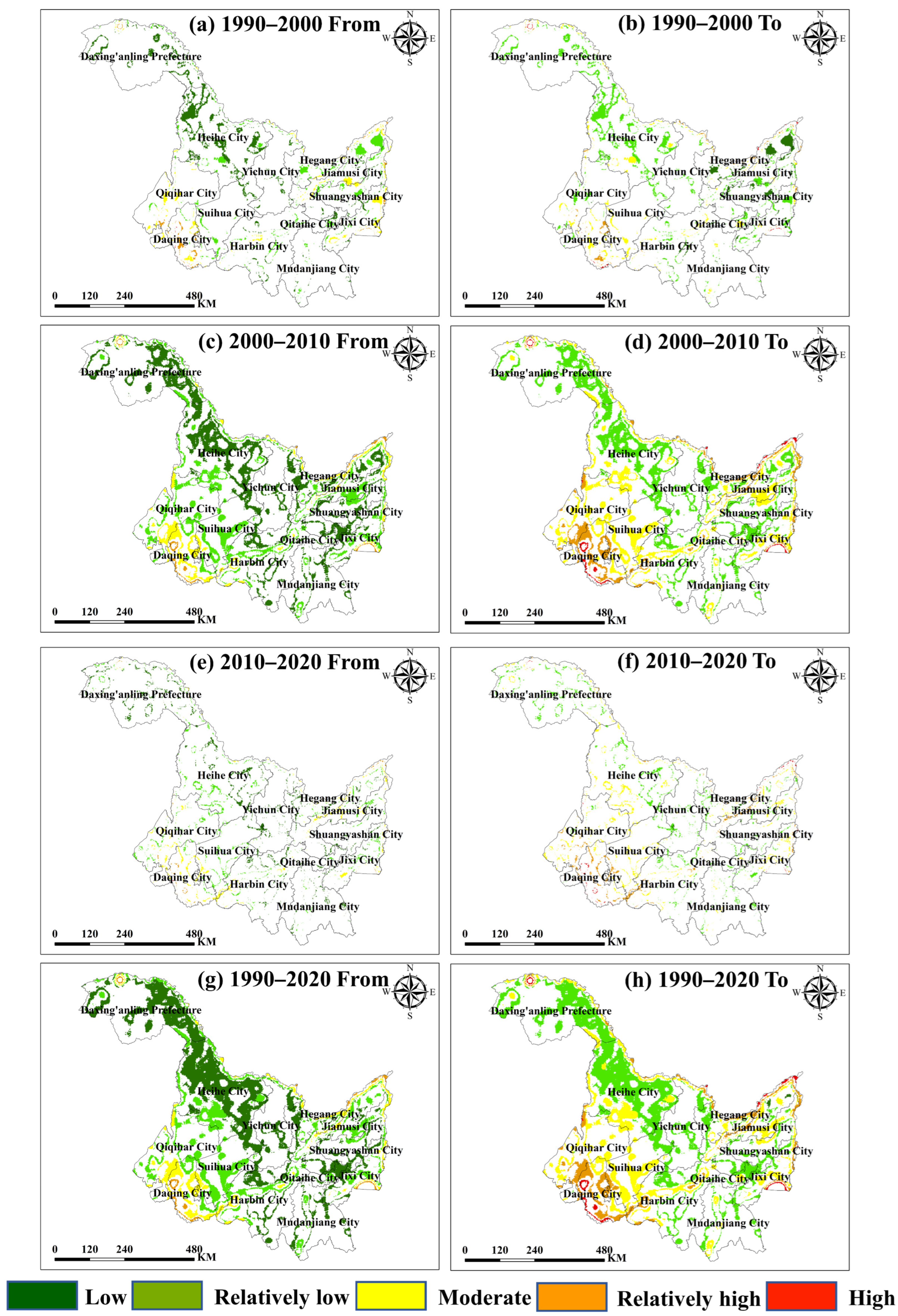
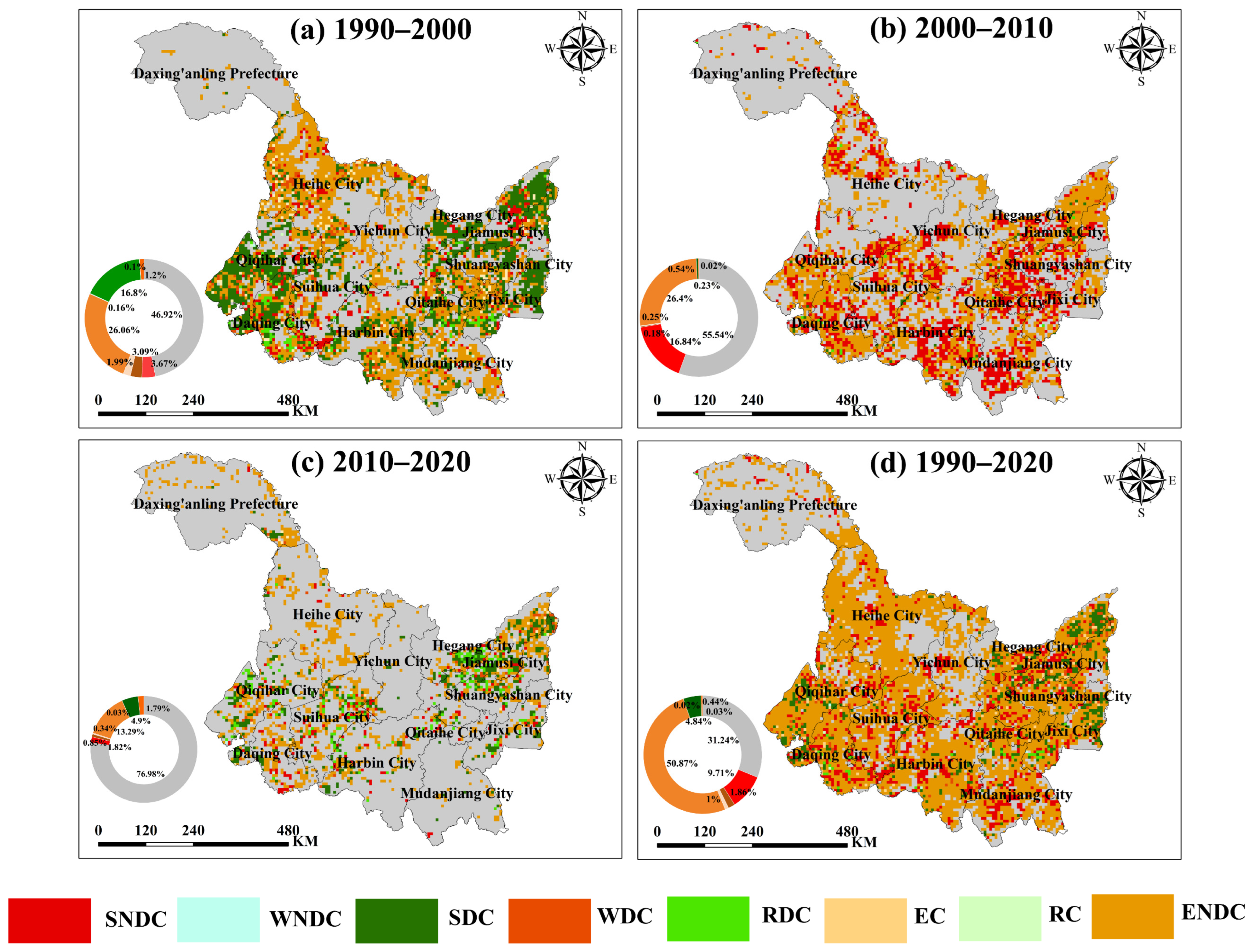
3.5. Decoupling Analysis Between the LUI and ERI in Heilongjiang Province

From 1990 to 2020, most areas of Heilongjiang Province exhibited ENDC (expansive negative decoupling), where the ERI increased with the increase in the LUI, while the rate of increase in the ERI was greater than that of the LUI (Figure 17). The SNDC (strong negative decoupling) areas were predominantly located in Suihua, Harbin, Mudanjiang, and Jiamusi. In these areas, the ERI increases as the LUI decreases. The SDC (strong decoupling) areas were primarily located in Qiqihar, Jiamusi, and Jixi, where the ERI decreases as the LUI increases. From 1990 to 2000, the ENDC and SDC predominated in Heilongjiang Province. The ENDC was predominantly located in Heihe, Harbin, Mudanjiang, and Qitaihe, while the SDC was primarily distributed in Qiqihar, Daqing, Hegang, Jiamusi, and Jixi. The RDC (recessive decoupling) areas were primarily located in Daqing and Jixi. From 2000 to 2010, the ENDC and SNDC predominated in Heilongjiang Province. The ENDC was predominantly located in Qiqihar, Daqing, Harbin, and Jiamusi, while the SNDC was primarily distributed in Harbin, Mudanjiang, and Qitaihe. Between 2010 and 2020, most regions exhibited no decoupling relationship. The ENDC was primarily located in Heihe, Qiqihar, Daqing, Jiamusi, and Shuangyashan, while the SDC was predominantly located in Jiamusi and Hegang.

4. Discussion

This study demonstrates that most regions of Heilongjiang Province exhibit low and relatively low ecological risk, but moderate- and higher-ecological-risk areas have steadily increased from 1990 to 2020, with their overall proportion rising by 10.62%. Notably, areas with relatively high ecological risk were predominantly located in Daqing and Qiqihar, situated in the southwestern part of the province. This finding is consistent with the western region (Qiqihar, Daqing, and Harbin) being characterized by pronounced ecological vulnerability [60]. This phenomenon is closely related to the complex land use patterns in these areas—large-scale oil extraction, urban expansion, and agricultural intensification have led to increased ecological fragmentation, confirming the conclusion of the ecological fragility of the Songnen Plain, while further elucidating the specific mechanisms through which industrial activities influence the environment [61]. Similarly, the U.S. Corn Belt, as a globally important agricultural region, also faces ecosystem pressures caused by farmland expansion and urbanization, such as reductions in vegetation cover, soil degradation, and declines in ecosystem stability [62,63]. Studies in the U.S. Corn Belt have emphasized the impacts of agricultural production activities and urban expansion on soil organic carbon stocks, ecological connectivity, and species diversity [64,65,66], revealing the vulnerability of ecosystem services in agricultural areas. In contrast, the ERI in Heilongjiang Province is more prominently manifested as increased ecological fragmentation and the expansion of localized vulnerable zones driven by industrial activities and agricultural intensification. The comparison between these two regions highlights the common ecological pressures driven by land use changes in agricultural zones, while also reflecting differences in the ERI patterns caused by variations in industrial structure and land use characteristics.

The analysis of the driving mechanisms of the ERI reveals that natural factors (the NDVI, precipitation, and DEM) form the basis of spatial differentiation, while human activities exacerbate risk accumulation through economic development. For example, Yichun and Mudanjiang in the Daxing’anling region maintain low risk levels due to high altitude forest cover, supporting the role of forests as carbon sinks [67]. In contrast, Daqing and Qiqihar, with flat terrain, low vegetation cover, and the overlay of oil industry activities and urban expansion, form high-risk areas. Interaction detection revealed that the synergistic effects of natural and human factors (such as the POP and temperature) significantly outweigh the influence of any single factor, aligning with the observed threshold effects of land development [68]. This dual driving feature is further emphasized in the decoupling analysis: although the growth rate of the LUI slowed from 2010 to 2020, industrial cities such as Daqing still exhibit the ENDC due to historical land use inertia, indicating that ecological recovery lags behind policy regulation [69].

The spatiotemporal evolution of decoupling types between the LUI and ERI reveals regional differences in sustainable development capabilities: the SDC in Qiqihar and Jiamusi is attributed to the adoption of precision agriculture technology, whereas the SNDC in Suihua and Harbin reflects the ecological debt resulting from past extensive land use. Notably, high-risk areas show a spatial correlation coefficient of 0.76 with identified carbon emission hotspots [70]. As energy bases, land use changes in Daqing and Qiqihar not only contributed to the increase in the ERI but also heighten carbon neutrality challenges due to the loss of vegetation carbon sinks [71]. This “risk emission” coupling effect highlights the need for future ERI management to be integrated into the carbon budget accounting framework. Moreover, ecological resilience and carbon sink potential should be enhanced simultaneously through land space optimization, such as the ecological restoration of industrial and mining lands and the construction of forest city networks [72].

At the same time, the decoupling results reveal a clear temporal lag in the ERI response. While the LUI experienced the most dramatic changes between 1990 and 2000, the most pronounced increases in the ERI occurred during 2000–2010, followed by a markedly slower rise from 2010 to 2020. This temporal mismatch indicates that the nationwide Grain for Green Program, launched in 2002, played a pivotal role in improving ecological conditions across Heilongjiang Province [73,74]. However, due to the inherent delay in ecosystem recovery processes, the beneficial effects of this policy were not immediately reflected in the LUI and ERI relationship. Instead, the ERI stabilized or even declined in many areas despite ongoing land development from 2010 to 2020 [75,76]. This delayed response underscores that ecological restoration policies require long-term implementation to yield measurable outcomes [77]. The spatial overlap between policy-targeted regions and areas that transitioned toward strong or stable decoupling further supports this conclusion, indicating that reforestation efforts effectively enhanced vegetation cover, reduced landscape fragmentation, and bolstered ecosystem resilience [78]. These findings highlight that successful ecological governance depends not only on moderating the LUI but also on sustained policy commitment and continuous environmental monitoring. Regions that have achieved effective decoupling as a result of ecological restoration should be viewed as critical reference models for future land use planning. Scaling up restoration efforts, particularly in ecologically fragile or marginal areas, may help mitigate the negative impacts of land development while contributing to carbon sequestration and advancing regional sustainability objectives.

Based on the current study results, the targeted adjustments under different future development scenarios are proposed as follows: (1) Under the natural development scenario, priority should be given to ecological restoration and industrial pollution control in high-risk areas such as Daqing and Qiqihar. These industrial cities have experienced significant ecological fragmentation due to oil extraction and urban expansion and require coordination between land development and ecological protection. (2) Under the farmland protection scenario, efforts should focus on reducing farmland fragmentation and promoting precision agriculture. In areas such as Qiqihar and Jiamusi, where sustainable decoupling between the LUI and ERI has already emerged, such strategies can support more efficient land use while further mitigating the ERI. (3) Under the ecological conservation scenario, given that the NDVI and DEM are the primary natural driving factors of the ERI, it is crucial to protect high-altitude forests and enhance ecological connectivity, especially in Daxing’anling Prefecture. This can be achieved by strengthening forest conservation and afforestation policies, restricting industrial and urban expansion in ecologically fragile areas, and establishing ecological corridors to improve carbon sequestration capacity and regional ecological resilience.

This study elucidates the key driving factors of the ERI in Heilongjiang Province over the period from 1990 to 2020 by analyzing the impact of both natural and socioeconomic factors. Although this study considered certain socioeconomic factors, it may not fully capture the broader human activities influencing the ERI, such as land protection policies, urbanization trends, and agricultural practices. These factors were critical in shaping land use patterns and their associated environmental impacts. Therefore, future studies could integrate granular socioeconomic data (e.g., land tenure systems and subsidy policies) to disentangle governance–ecology linkages. Additionally, the current assessment relies on remote sensing and modeled indicators without field validation, which may limit ecological realism. Future work should also integrate ground-based ecological data (e.g., biodiversity and soil quality) to improve evaluation robustness. To capture finer temporal dynamics, annual-scale analysis should be considered, along with dynamic weight-setting approaches (e.g., entropy or AHP methods) to reflect the evolving influence of different drivers on the LUI and ERI over time.

5. Conclusions

This study evaluates the spatiotemporal evolution of the ERI and its main driving factors in Heilongjiang Province from 1990 to 2020 and analyzed the decoupling relationship between the LUI and ERI. The results are as follows: (1) The primary land use types in Heilongjiang Province are farmland and woodland. Over the past three decades, there has been a significant increase in farmland and construction land, while woodland and grassland have substantially decreased, mainly due to their conversion to farmland. Particularly, Daqing exhibits complex land use types, while Heihe and Qiqihar have experienced more drastic changes. (2) From 1992 to 2022, Heilongjiang Province experienced rapid land development, leading to a significant cumulative effect on the ERI, with the LUI having grown at an average annual rate of 1.2%. Spatially, risk hotspots have emerged in the southwest industrial corridor (Daqing and Qiqihar) and northeast resource-based cities (Jixi), with moderate- and higher-ecological-risk areas increasing by 10.62%. (3) A 7 km × 7 km resolution is identified as optimal for ERI assessment, effectively capturing its spatial heterogeneity. The mechanism driving risk exhibits phased characteristics: in the 1990s, DEM was the dominant factor (q = 0.48), while post-2000, vegetation restoration policies have increased the influence of the NDVI (q = 0.52). (4) While ENDC is dominant (62.3%), the presence of SDC in cities like Qiqihar and Jiamusi demonstrates that enhancing arable land protection and wetland restoration can mitigate risks while improving land productivity, providing empirical insights for similar regions. Our findings provide actionable insights for optimizing the ‘Ecological Redline Policy’ in Northeast China through grid-scale risk zoning.

References

1. Luo, F.; Liu, Y.; Peng, J.; Wu, J. Assessing urban landscape ecological risk through an adaptive cycle framework. Landsc. Urban Plan. 2018, 180, 125–134. [Google Scholar] [CrossRef]
2. Yin, R.; Yin, G. China’s primary programs of terrestrial ecosystem restoration: Initiation, implementation, and challenges. Environ. Manag. 2010, 45, 429–441. [Google Scholar] [CrossRef] [PubMed]
3. Forbes, V.E.; Galic, N. Next-generation ecological risk assessment: Predicting risk from molecular initiation to ecosystem service delivery. Environ. Int. 2016, 91, 215–219. [Google Scholar] [CrossRef] [PubMed]
4. Lal, P.; Shekhar, A.; Kumar, A. Quantifying temperature and precipitation change caused by land cover change: A case study of India using the WRF model. Front. Environ. Sci. 2021, 9, 766328. [Google Scholar] [CrossRef]
5. Anagonou, S.P.G.; Ewemoje, T.A.; Toyi, S.S.M.; Olubode, O.S. Landscape ecological risk assessment and transformation processes in the Guinean-Congolese climate zone in Benin Republic. Remote Sens. Appl. Soc. Environ. 2023, 31, 100985. [Google Scholar] [CrossRef]
6. Chen, J.; Dong, B.; Li, H.; Zhang, S.; Peng, L.; Fang, L.; Zhang, C.; Li, S. Study on landscape ecological risk assessment of Hooded Crane breeding and overwintering habitat. Environ. Res. 2020, 187, 109649. [Google Scholar] [CrossRef]
7. Zeng, C.; Zhang, A.; Liu, L.; Liu, Y. Administrative restructuring and land-use intensity—A spatial explicit perspective. Land Use Policy 2017, 67, 190–199. [Google Scholar] [CrossRef]
8. Chen, Y.; Li, X.; Tian, Y.; Tan, M. Structural change of agricultural land use intensity and its regional disparity in China. J. Geogr. Sci. 2009, 19, 545–556. [Google Scholar] [CrossRef]
9. Ma, J.; Khromykh, V.; Wang, J.; Zhang, J.; Li, W.; Zhong, X. A landscape-based ecological hazard evaluation and characterization of influencing factors in Laos. Front. Ecol. Evol. 2023, 11, 1276239. [Google Scholar] [CrossRef]
10. Ran, P.; Hu, S.; Frazier, A.E.; Qu, S.; Yu, D.; Tong, L. Exploring changes in landscape ecological risk in the Yangtze River Economic Belt from a spatiotemporal perspective. Ecol. Indic. 2022, 137, 108744. [Google Scholar] [CrossRef]
11. Canelas, J.V.; Pereira, H.M. Impacts of land-use intensity on ecosystems stability. Ecol. Model. 2022, 472, 110093. [Google Scholar] [CrossRef]
12. Peng, J.; Dang, W.; Liu, Y.; Zong, M.; Hu, X. Review on landscape ecological risk assessment. Acta Geogr. Sin. 2015, 70, 664–677. (In Chinese) [Google Scholar]
13. Li, Z.; Jiang, W.; Wang, W.; Chen, Z.; Ling, Z.; Lv, J. Ecological risk assessment of the wetlands in Beijing-Tianjin-Hebei urban agglomeration. Ecol. Indic. 2020, 117, 106677. [Google Scholar] [CrossRef]
14. Li, J.; Pu, R.; Gong, H.; Luo, X.; Ye, M.; Feng, B. Evolution characteristics of landscape ecological risk patterns in coastal zones in Zhejiang Province, China. Sustainability 2017, 9, 584. [Google Scholar] [CrossRef]
15. Wang, H.; Liu, X.; Zhao, C.; Chang, Y.; Liu, Y.; Zang, F. Spatial-temporal pattern analysis of landscape ecological risk assessment based on land use/land cover change in Baishuijiang National nature reserve in Gansu Province, China. Ecol. Indic. 2021, 124, 107454. [Google Scholar] [CrossRef]
16. Zhang, X.; Du, H.; Wang, Y.; Chen, Y.; Ma, L.; Dong, T. Watershed landscape ecological risk assessment and landscape pattern optimization: Take Fujiang River Basin as an example. Hum. Ecol. Risk Assess. 2021, 27, 2254–2276. [Google Scholar] [CrossRef]
17. Wang, B.; Ding, M.; Li, S.; Liu, L.; Ai, J. Assessment of landscape ecological risk for a cross-border basin: A case study of the Koshi River Basin, central Himalayas. Ecol. Indic. 2020, 117, 106621. [Google Scholar] [CrossRef]
18. Li, Q.; Wang, L.; Du, G.; Faye, B.; Li, Y.; Li, J.; Liu, W.; Qu, S. Dynamic Variation of Ecosystem Services Value under Land Use/Cover Change in the Black Soil Region of Northeastern China. Int. J. Environ. Res. Public Health 2022, 19, 7533. [Google Scholar] [CrossRef]
19. Zhang, Y.; Bian, Z.; Guo, X.; Wang, C.; Guan, D. Strategic land management for ecosystem Sustainability: Scenario insights from the Northeast black soil region. Ecol. Indic. 2024, 168, 112784. [Google Scholar] [CrossRef]
20. Jiang, Y.; Du, G.; Teng, H.; Wang, J.; Li, H. Multi-Scenario Land Use Change Simulation and Spatial Response of Ecosystem Service Value in Black Soil Region of Northeast China. Land 2023, 12, 962. [Google Scholar] [CrossRef]
21. Griffin, T.; Conrad, Z.; Peters, C.; Ridberg, R.; Tyler, E.P. Regional self-reliance of the Northeast food system. Renew. Agric. Food Syst. 2014, 30, 349–363. [Google Scholar] [CrossRef]
22. Wang, Z.; Liu, B.; Wang, X.; Gao, X.; Liu, G. Erosion effect on the productivity of black soil in Northeast China. Sci. China Ser. D Earth Sci. 2009, 52, 1005–1021. [Google Scholar] [CrossRef]
23. Niu, L.; Shao, Q.; Ning, J.; Liu, S.; Zhang, X.; Zhang, T. The assessment of ecological restoration effects on Beijing-Tianjin Sandstorm Source Control Project area during 2000–2019. Ecol. Eng. 2023, 186, 106831. [Google Scholar] [CrossRef]
24. Gao, J.; Liu, Y. Climate warming and land use change in Heilongjiang Province, Northeast China. Appl. Geogr. 2011, 31, 476–482. [Google Scholar] [CrossRef]
25. Karimian, H.; Zou, W.; Chen, Y.; Xia, J.; Wang, Z. Landscape ecological risk assessment and driving factor analysis in Dongjiang river watershed. Chemosphere 2022, 307, 135835. [Google Scholar] [CrossRef]
26. Deng, G.; Jiang, H.; Zhu, S.; Wen, Y.; He, C.; Wang, X.; Sheng, L.; Guo, Y.; Cao, Y. Projecting the response of ecological risk to land use/land cover change in ecologically fragile regions. Sci. Total Environ. 2024, 914, 169908. [Google Scholar] [CrossRef]
27. Du, L.; Dong, C.; Kang, X.; Qian, X.; Gu, L. Spatiotemporal evolution of land cover changes and landscape ecological risk assessment in the Yellow River Basin, 2015–2020. J. Environ. Manag. 2023, 332, 117149. [Google Scholar] [CrossRef]
28. Bhattachan, A.; Emanuel, R.E.; Ardón, M.; Bernhardt, E.S.; Anderson, S.M.; Stillwagon, M.G.; Ury, E.A.; BenDor, T.K.; Wright, J.P. Evaluating the effects of land-use change and future climate change on vulnerability of coastal landscapes to saltwater intrusion. Elem. Sci. Anthr. 2018, 6, 62. [Google Scholar] [CrossRef]
29. Xing, L.; Hu, M.; Wang, Y. Integrating ecosystem services value and uncertainty into regional ecological risk assessment: A case study of Hubei Province, Central China. Sci. Total Environ. 2020, 740, 140126. [Google Scholar] [CrossRef]
30. Zhang, W.; Chang, W.J.; Zhu, Z.C.; Hui, Z. Landscape ecological risk assessment of Chinese coastal cities based on land use change. Appl. Geogr. 2020, 117, 102174. [Google Scholar] [CrossRef]
31. Li, Y.; Chen, Y.; Karimian, H.; Tao, T. Spatiotemporal analysis of air quality and its relationship with meteorological factors in the Yangtze River Delta. J. Elementol. 2020, 25, 1059–1075. [Google Scholar] [CrossRef]
32. Wang, Y.; Geng, Q.; Si, X.; Kan, L. Coupling and coordination analysis of urbanization, economy and environment of Shandong Province, China. Environ. Dev. Sustain. 2020, 23, 10397–10415. [Google Scholar] [CrossRef]
33. Wang, H.; Qin, F.; Xu, C.; Li, B.; Guo, L.; Wang, Z. Evaluating the suitability of urban development land with a Geodetector. Ecol. Indic. 2021, 123, 107339. [Google Scholar] [CrossRef]
34. Wang, Y.; Wang, X.; Chen, W.; Qiu, L.; Wang, B.; Niu, W. Exploring the path of inter-provincial industrial transfer and carbon transfer in China via combination of multi-regional input–output and geographically weighted regression model. Ecol. Indic. 2021, 125, 107547. [Google Scholar] [CrossRef]
35. Wang, J.F.; Li, X.H.; Christakos, G.; Liao, Y.L.; Zhang, T.; Gu, X.; Zheng, X.Y. Geographical detectors-based health risk assessment and its application in the neural tube defects study of the Heshun Region, China. Int. J. Geogr. Inf. Sci. 2010, 24, 107–127. [Google Scholar] [CrossRef]
36. Wang, Y.; Zhang, Z.; Chen, X. Quantifying influences of natural and anthropogenic factors on vegetation changes based on Geodetector: A Case Study in the Poyang Lake Basin, China. Remote Sens. 2021, 13, 5081. [Google Scholar] [CrossRef]
37. Gao, F.; Li, S.; Tan, Z.; Wu, Z.; Zhang, X.; Huang, G.; Huang, Z. Understanding the modifiable areal unit problem in dockless bike sharing usage and exploring the interactive effects of built environment factors. Int. J. Geogr. Inf. Sci. 2021, 35, 1905–1925. [Google Scholar] [CrossRef]
38. Song, Y.; Wang, J.; Ge, Y.; Xu, C. An optimal parameters-based geographical detector model enhances geographic characteristics of explanatory variables for spatial heterogeneity analysis: Cases with different types of spatial data. GISci. Remote Sens. 2020, 57, 593–610. [Google Scholar] [CrossRef]
39. Li, D.; He, L.; Qu, J.; Xu, X. Spatial evolution of cultivated land in the Heilongjiang Province in China from 1980 to 2015. Environ. Monit. Assess. 2022, 194, 444. [Google Scholar] [CrossRef]
40. An, Y.; Liu, S.; Sun, Y.; Shi, F.; Zhao, S. Negative effects of farmland expansion on multi-species landscape connectivity in a tropical region in Southwest China. Agric. Syst. 2020, 179, 102766. [Google Scholar] [CrossRef]
41. Millard, J.; Outhwaite, C.L.; Kinnersley, R.; Freeman, R.; Gregory, R.D.; Adedoja, O.; Gavini, S.; Kioko, E.; Kuhlmann, M.; Ollerton, J. Global effects of land-use intensity on local pollinator biodiversity. Nat. Commun. 2021, 12, 2902. [Google Scholar] [CrossRef]
42. Xie, Y.; Liu, Z.; Zhao, J.; Li, Y.; Zhang, L. Analysis of Landuse Dynamic in Typical Blacksoil Region Based on GIS and RS—A Case Study of Hailun County. Sci. Geogr. Sin. 2010, 30, 428–434. (In Chinese) [Google Scholar] [CrossRef]
43. Qi, Y.; Wang, R.; Shen, P.; Ren, S.; Hu, Y. Impacts of Land Use Intensity on Ecosystem Services: A Case Study in Harbin City, China. Sustainability 2023, 15, 14877. [Google Scholar] [CrossRef]
44. Xiang, J.; Li, X.; Xiao, R.; Wang, Y. Effects of land use transition on ecological vulnerability in poverty-stricken mountainous areas of China: A complex network approach. J. Environ. Manag. 2021, 297, 113206. [Google Scholar] [CrossRef]
45. Liu, D.; Chen, H.; Zhang, H.; Geng, T.; Shi, Q. Spatiotemporal evolution of landscape ecological risk based on geomorphological regionalization during 1980–2017: A case study of Shaanxi Province, China. Sustainability 2020, 12, 941. [Google Scholar] [CrossRef]
46. Peng, J.; Zong, M.; Hu, Y.; Liu, Y.; Wu, J. Assessing landscape ecological risk in a mining city: A case study in Liaoyuan City, China. Sustainability 2015, 7, 8312–8334. [Google Scholar] [CrossRef]
47. Zhang, F.; Yushanjiang, A.; Wang, D. Ecological risk assessment due to land use/cover changes (LUCC) in Jinghe County, Xinjiang, China from 1990 to 2014 based on landscape patterns and spatial statistics. Environ. Earth Sci. 2018, 77, 491. [Google Scholar] [CrossRef]
48. Gao, B.; Li, C.; Wu, Y.; Zheng, K.; Wu, Y. Landscape ecological risk assessment and influencing factors in ecological conservation area in Sichuan-Yunnan provinces, China. Chin. J. Appl. Ecol. 2021, 32, 1603–1613. (In Chinese) [Google Scholar]
49. Sui, L.; Yan, Z.; Li, K.; Wang, C.; Shi, Y.; Du, Y. Prediction of ecological security network in Northeast China based on landscape ecological risk. Ecol. Indic. 2024, 160, 111783. [Google Scholar] [CrossRef]
50. Qu, C.; Li, W.; Xu, J.; Shi, S. Blackland conservation and utilization, carbon storage and ecological risk in green space: A case study from Heilongjiang Province in China. Int. J. Environ. Res. Public Health 2023, 20, 3154. [Google Scholar] [CrossRef]
51. Bian, Z.; Liu, B.; Guan, D. Landscape Ecological Risk Assessment for the Black Soil Region in Northeast China Based on Land Use Change. J. Shenyang Agric. Univ. 2025, 56, 140–155. (In Chinese) [Google Scholar] [CrossRef]
52. Rangel-Buitrago, N.; Neal, W.J.; de Jonge, V.N. Risk assessment as tool for coastal erosion management. Ocean Coast. Manag. 2020, 186, 105099. [Google Scholar] [CrossRef]
53. Zhang, W.; Sun, X.; Shan, R.; Liu, F. Spatio-temporal quantification of landscape ecological risk changes and its driving forces in the Nansihu Lake basin during 1975–2018. Ecol. Sci. 2020, 39, 172–181. [Google Scholar] [CrossRef]
54. Tapio, P. Towards a theory of decoupling: Degrees of decoupling in the EU and the case of road traffic in Finland between 1970 and 2001. Transp. Policy 2005, 12, 137–151. [Google Scholar] [CrossRef]
55. Huo, T.; Ma, Y.; Yu, T.; Cai, W.; Liu, B.; Ren, H. Decoupling and decomposition analysis of residential building carbon emissions from residential income: Evidence from the provincial level in China. Environ. Impact Assess. Rev. 2021, 86, 106487. [Google Scholar] [CrossRef]
56. Liu, Q.; Wang, Z. Coupling and Decoupling Situation of Tourism Economic Development and Eeological Environment Pressure of Urban Agglomeration in the Middle Reaches of the Yangtze River. Geogr. Geo-Inf. Sci. 2021, 37, 128–134. (In Chinese) [Google Scholar] [CrossRef]
57. Zhang, X.; Zhou, C.; Li, Y.; Zhou, L.; Ren, M.; Zhao, Y. Temporal-spatial characteristics and dynamic decoupling process of tourism economic development and eco-environmental pressure in provinces of the Yellow River Basin. J. Desert Res. 2022, 42, 241–250. (In Chinese) [Google Scholar] [CrossRef]
58. Huang, Z.; Chen, Y.; Wu, Z. Spatiotemporal charactersitics of decoupling between land surface thermal environment and ecosystem service value in Pearl River Delta Urban Agglomeration, China. Chin. J. Appl. Ecol. 2022, 33, 1993–2000. [Google Scholar] [CrossRef]
59. Wang, X.; Zhang, S.; Ding, Z.; Hou, H.; Wu, Q.; Wang, Y.; Li, Y. Carbon ecological security assessment based on the decoupling relationship between carbon balance pressure and ecological quality in Xuzhou City, China. Environ. Sci. Pollut. Res. 2023, 31, 7428–7442. [Google Scholar] [CrossRef]
60. Li, Y.; Liu, J.; Zhu, Y.; Wu, C.; Zhang, Y. Spatiotemporal Differentiation and Attribution Analysis of Ecological Vulnerability in Heilongjiang Province, China, 2000–2020. Sustainability 2025, 17, 2239. [Google Scholar] [CrossRef]
61. Wang, H.; Zhang, C.; Yao, X.; Yun, W.; Ma, J.; Gao, L.; Li, P. Scenario simulation of the tradeoff between ecological land and farmland in black soil region of Northeast China. Land Use Policy 2022, 114, 105991. [Google Scholar] [CrossRef]
62. Schneider, A.; Logan, K.E.; Kucharik, C.J. Impacts of Urbanization on Ecosystem Goods and Services in the U.S. Corn Belt. Ecosystems 2012, 15, 519–541. [Google Scholar] [CrossRef]
63. Thaler, E.A.; Larsen, I.J.; Yu, Q. The extent of soil loss across the US Corn Belt. Proc. Natl. Acad. Sci. USA 2021, 118, e1922375118. [Google Scholar] [CrossRef] [PubMed]
64. Marull, J.; Cunfer, G.; Sylvester, K.; Tello, E. A landscape ecology assessment of land-use change on the Great Plains-Denver (CO, USA) metropolitan edge. Reg. Environ. Change 2018, 18, 1765–1782. [Google Scholar] [CrossRef]
65. Phillips, D.L.; Lee, J.J.; Dodson, R.F. Sensitivity of the US Corn Belt to Climate Change and Elevated CO2: II. Soil Erosion and Organic Carbon. Agric. Syst. 1996, 52, 481–502. [Google Scholar] [CrossRef]
66. Zhang, Y.; Marx, E.; Williams, S.; Gurung, R.; Ogle, S.; Horton, R.; Bader, D.; Paustian, K. Adaptation in U.S. Corn Belt increases resistance to soil carbon loss with climate change. Sci. Rep. 2020, 10, 13799. [Google Scholar] [CrossRef]
67. Qiao, B.; Yang, H.; Cao, X.; Zhou, B.; Wang, N. Driving mechanisms and threshold identification of landscape ecological risk: A nonlinear perspective from the Qilian Mountains, China. Ecol. Indic. 2025, 173, 113342. [Google Scholar] [CrossRef]
68. Wu, X.; Cui, J. Spatiotemporal analysis of coupling coordination between urbanization and ecological efficiency of cultivated land use in Heilongjiang Province. Agric. Technol. 2025, 45, 160–165. (In Chinese) [Google Scholar]
69. Lu, S.; Chen, N.; Guan, X.; Chen, G. Comprehensive Assessment of the Agricultural Eco-Economic System in Heilongjiang Province Based on GIS and Energy Analysis Theory. J. Ecol. Rural Environ. 2016, 32, 879–886. (In Chinese) [Google Scholar]
70. Guo, R.; Wu, X.; Wu, T.; Dai, C. Spatial–Temporal Pattern Characteristics and Impact Factors of Carbon Emissions in Production–Living–Ecological Spaces in Heilongjiang Province, China. Land 2023, 12, 1153. [Google Scholar] [CrossRef]
71. Zhang, H.; He, Z.; Zhang, L.; Cong, R.; Wei, W. Spatial–Temporal Changes and Driving Factor Analysis of Net Ecosystem Productivity in Heilongjiang Province from 2010 to 2020. Land 2024, 13, 1316. [Google Scholar] [CrossRef]
72. Zhang, Q.; Kou, C.; Gao, W. Coupling coordination relationship of forestry industry development and ecological environment: Evidence from Heilongjiang Province. Front. Environ. Sci. 2024, 12, 1375657. [Google Scholar] [CrossRef]
73. Xian, J.; Xia, C.; Cao, S. Cost–benefit analysis for China’s Grain for Green Program. Ecol. Eng. 2020, 151, 105850. [Google Scholar] [CrossRef]
74. Wu, X.; Wang, S.; Fu, B.; Feng, X.; Chen, Y. Socio-ecological changes on the Loess Plateau of China after Grain to Green Program. Sci. Total Environ. 2019, 678, 565–573. [Google Scholar] [CrossRef] [PubMed]
75. Qiao, Y.; Xu, W.; Liu, K.; Pei, W.; Wang, Z.; Han, X.; Zhang, H. Spatio-temporal evolution of vegetation NPP in Heilongijiang Province based onthe multi-scale geographically weighted regression model. Acta Ecol. Sin. 2025, 45, 4878–4888. (In Chinese) [Google Scholar] [CrossRef]
76. Li, Y.; Zhao, N.; Zhang, Y.; Monika, S.; Du, G. Evolution in Land-Habitat Quality in Black Soil Area of Northeast China and Muti-Scenario Forecasting: The Study of Heilongjiang Province. Environ. Sci. 2025, 1–21. (In Chinese) [Google Scholar] [CrossRef]
77. Cao, S.; Liu, Y.; Su, W.; Zheng, X.; Yu, Z. The net ecosystem services value in mainland China. Sci. China Earth Sci. 2018, 61, 595–603. [Google Scholar] [CrossRef]
78. Peng, J.; Hu, X.; Wang, X.; Meersmans, J.; Liu, Y.; Qiu, S. Simulating the impact of Grain-for-Green Programme on ecosystem services trade-offs in Northwestern Yunnan, China. Ecosyst. Serv. 2019, 39, 100998. [Google Scholar] [CrossRef]
Figure 1. Overview of the study area of Heilongjiang Province in Northeast China.
Remotesensing 17 02243 g001
Figure 2. The driving factors of the ERI in Heilongjiang Province.
Remotesensing 17 02243 g002
Figure 3. Framework of the study.
Remotesensing 17 02243 g003
Figure 4. Land use transfer matrix in Heilongjiang Province from 1990 to 2020.
Remotesensing 17 02243 g004
Figure 5. Spatial distribution of land use in Heilongjiang Province from 1990 to 2020.
Remotesensing 17 02243 g005
Figure 6. Temporal and spatial changes in land use in Heilongjiang Province from 1990 to 2020.
Remotesensing 17 02243 g006
Figure 7. Spatial distribution of LUI in Heilongjiang Province from 1990 to 2020.
Remotesensing 17 02243 g007
Figure 8. Spatial distribution changes in LUI in Heilongjiang Province from 1990 to 2020.
Remotesensing 17 02243 g008
Figure 9. Spatial distribution of ERI in Heilongjiang Province at the different scale resolutions.
Remotesensing 17 02243 g009
Figure 10. Changes in the Moran’s I index of ERI in Heilongjiang Province at different scale resolutions.
Remotesensing 17 02243 g010
Figure 11. Spatial distribution of ERI in Heilongjiang Province from 1990 to 2020.
Remotesensing 17 02243 g011
Figure 12. Spatial distribution changes in ERI in Heilongjiang Province from 1990 to 2020.
Remotesensing 17 02243 g012
Figure 13. Track map depicting the ecological risk center of gravity in Heilongjiang Province from 1990 to 2020.
Remotesensing 17 02243 g013
Figure 14. Local spatial autocorrelation agglomeration of ecological risk in Heilongjiang Province from 1990 to 2020.
Remotesensing 17 02243 g014
Figure 15. The detection of driving factors for the spatial differentiation of ecological risk in Heilongjiang Province from 2000 to 2020. (Note: X1, GDP; X2, POP; X3, distance to railway; X4, distance to road; X5, distance to river; X6, annual total precipitation; X7, annual average temperature; X8, NDVI; X9, DEM; X10, slope gradient; X11, slope aspect.)
Remotesensing 17 02243 g015
Figure 16. Interaction of the driving factors influencing the spatial differentiation of the ecological risk in Heilongjiang Province from 1990 to 2020. (Note: X1, GDP; X2, POP; X3, distance to railway; X4, distance to road; X5, distance to river; X6, annual total precipitation; X7, annual average temperature; X8, NDVI; X9, DEM; X10, slope gradient; X11, slope aspect.)
Remotesensing 17 02243 g016
Figure 17. Spatial distribution of decoupling in Heilongjiang Province from 1990 to 2020. (Note: SNDC, Strong negative decoupling; WNDC, Weak negative decoupling; SDC, Strong decoupling; WDC, Weak decoupling; RDC, Recessive decoupling; EC, Expansive coupling; RC, Recessive coupling; ENDC, Expansive negative decoupling).
Remotesensing 17 02243 g017