An Improved Size and Direction Adaptive Filtering Method for Bathymetry Using ATLAS ATL03 Data

Abstract

The Advanced Topographic Laser Altimeter System (ATLAS) on the Ice, Cloud, and Land Elevation Satellite-2 (ICESat-2) employs a photon-counting detection mode with a 532 nm laser to obtain high-precision Earth surface elevation data and offers a new remote sensing method for nearshore bathymetry. The key issues in using ATLAS ATL03 data for bathymetry are achieving automatic and accurate extraction of signal photons in different water environments. Especially for areas with sharply fluctuating topography, the interaction of various impacts, such as topographic fluctuations, sea waves, and laser pulse direction, can result in a sharp change in photon density and distribution at the seafloor, which can cause the signal photon detection at the seafloor to be misinterpreted or omitted during analysis. Therefore, an improved size and direction adaptive filtering (ISDAF) method was proposed for nearshore bathymetry using ATLAS ATL03 data. This method can accurately distinguish between the original photons located above the sea surface, on the sea surface, and the seafloor. The size and direction of the elliptical density filter kernel automatically adapt to the sharp fluctuations in topography and changes in water depth, ensuring precise extraction of signal photons from both the sea surface and the seafloor. To evaluate the precision and reliability of the ISDAF, ATLAS ATL03 data from different water environments and seafloor terrains were used to perform bathymetric experiments. Airborne LiDAR bathymetry (ALB) data were also used to validate the bathymetric accuracy and reliability. The experimental findings show that the ISDAF consistently exhibits effectiveness in detecting and retrieving signal photons, regardless of whether the seafloor terrain is stable or dynamic. After applying refraction correction, the high accuracy of bathymetry was evidenced by a strong coefficient of determination (R²) and a low root mean square error (RMSE) between the ICESat-2 bathymetry data and ALB data. This research offers a promising approach to advancing remote sensing technologies for precise nearshore bathymetric mapping, with implications for coastal monitoring, marine ecology, and resource management.

1. Introduction

The coastal zone serves as a bridge between various interactions between marine ecosystems and human activities, which is of great significance for the utilization of nearshore resources, guidance of human policy, and sustainability of ocean ecology [1,2]. The most up-to-date and precise seafloor topography provides indispensable geographic information for extensive coastal applications, including coastal erosion monitoring, geoarchaeological feature mapping, marine eutrophic treatment, and benthic habitat assessment [3,4,5]. However, the extensive shallow water areas surrounding coastal zones remain a formidable challenge for surveying and mapping, which is mainly caused by complex geographical, climatic, and marine environments.

Traditional bathymetric approaches include shipborne single/multibeam sonar systems, airborne LiDAR bathymetry (ALB) systems, and satellite-derived bathymetry (SDB) methods [6,7,8]. Although shipborne sonar systems offer high bathymetry accuracy, the measurement efficiency of this method sharply decreases in extremely shallow areas. The ALB system has a high bathymetry accuracy close to that of a sonar system, but is limited by factors such as the weather environment and airspace control conditions. Among the three bathymetry methods, the SDB method had the highest measurement efficiency; however, its measurement accuracy is the lowest, and bathymetric sample data, which are difficult to acquire, are necessary for distantly measured areas [9]. With the advancements in photon-counting methodologies, the utilization of photon-counting LiDAR has demonstrated several advantages for mapping and surveying [10,11,12]. The world’s inaugural photon-counting altimeter deployed on the Ice, Cloud, and Land Elevation Satellite-2 (ICESat-2) is known as the Advanced Topographic Altimeter System (ATLAS) [13,14,15]. It employs a green laser, allowing for the penetration of water and obtaining seafloor signals [16]. Therefore, this is the initial photon-counting LiDAR deployed in space to achieve nearshore bathymetry, providing a new opportunity for the efficient and worldwide acquisition of nearshore bathymetry and seafloor topography.

Various detection methods based on ATLAS ATL03 data have been proposed to extract signal photons and achieve measurements from different types of surfaces on Earth. These methods mainly consist of density-based models [17,18,19], contour active models [20,21], spatial statistical methods, and localized statistical analyses [22]. Currently, methods that use the local density and cluster of photons, such as the Bayes density cluster, density-based spatial clustering of applications with noise (DBSCAN), and ordering points to identify the clustering structure (OPTICS), have been widely adopted and used owing to their highly efficient and precise identification of signal photons. In nearshore bathymetry, the photon density decreases with increasing depth, and its distribution changes with different water depths and environments. Therefore, it is difficult to adapt traditional detection methods for nearshore bathymetry. Ma et al. utilized enhanced DBSCAN to extract photon signals from shallow marine areas [13], Hsu et al. used segmented median filtering for denoising and showcasing methods that were more effective in handling specific data than mean filtering [23], and Wang et al. introduced a photon-denoising method that incorporates an adaptable elevation-difference threshold [24]. However, these methods still require empirical threshold setting and manual intervention to attain satisfactory results. The adaptive variable ellipse filtering bathymetric method (AVEBM) method proposed by Chen et al. can efficiently eliminate these issues [25]; however, in addition to the characteristics of photon density and distribution caused by water depth and environment, the different reflectivities of various seafloor sediments and seafloor topographic changes can also result in changes in seafloor photon density and distributions, especially for sharp fluctuations in topography. In this situation, current methods may not fully account for the change in photon density and distribution due to these impacts. Cao et al. [26] identified this issue and proposed a size and direction adaptive filtering (SDAF) algorithm for extracting signal photons at the water surface and seafloor. However, when determining the orientation of the elliptical filter kernel, they fixed the ellipse rotation angle at 10 degrees, which prevented the accurate determination of the optimal ellipse angle. Consequently, in the final filtering result, numerous noise points were present near the seafloor signal photons.

To overcome these measurement problems, an improved size and direction adaptive filtering (ISDAF) method was proposed and validated to improve the precision and reliability of ICESat-2’s bathymetric measurements. In this method, the size and density thresholds of ellipse filtering can be adaptively adjusted as the water depth increases. For each seafloor photon, the direction of the ellipse filtering can also be automatically rotated and determined through the fluctuations and trends of the seafloor topography. Based on the elliptic filtering window and density threshold, the signal photons can be accurately detected and extracted. To assess the accuracy and reliability of this proposed method, experiments were performed in various regions within the South China Sea. The bathymetric outcomes were acquired utilizing airborne LiDAR bathymetry (ALB) and were then compared with the experimental results. Ultimately, by analyzing and comparing these findings, the accurate change in nearshore bathymetry was statistically calculated to investigate how fluctuations and trends in seafloor topography impact photon detection of ICESat-2.

This method offers a highly effective solution for accurate bathymetric measurement in challenging shallow-water environments, which are traditionally difficult to assess. Although it is designed to address the complexities of shallow water bathymetry, the approach is highly adaptable, offering the potential to scale to broader applications. With its capacity to generate precise, real-time bathymetric data, this method holds promise for improving safety in maritime navigation, enhancing environmental monitoring efforts, and supporting the sustainable management of coastal ecosystems worldwide. Furthermore, the ISDAF method’s reduced dependency on manual intervention and its adaptability to different water depths and terrains suggest that it could be applied in a wide range of environments, from shallow coastal waters to deeper, more dynamic marine regions. Its potential to integrate with other remote sensing technologies could further expand its global applicability, contributing to more efficient and accurate monitoring of marine and coastal areas on a global scale.

2. Materials and Methods

To achieve high-precision bathymetry using the ATLAS ATL03 datasets, the ISDAF model is initially applied to efficiently separate and extract signal photons from both the sea surface and the seafloor. After the photon extraction, a precise refraction correction is applied to the seafloor photons to account for the effects of sea surface fluctuations on the water column. This correction is achieved using the point-weight cubic polynomial (PWCP) model, ensuring the acquisition of accurate bathymetric data. The overall process is outlined in the flow diagram in Figure 1.

As shown in Figure 1, the flowchart illustrates the entire bathymetric process using the ATLAS ATL03 dataset. Initially, raw data containing photon-counting information from the ATLAS system is input into the processing pipeline. The process is divided into two main sections: the size and direction adaptive elliptical filtering and the point-weight cubic polynomial model.

In the size and direction adaptive elliptical filtering section, the first step involves regional photon separation. The raw data are divided into multiple segments along the elevation direction, and each slice is analyzed based on the number of photons it contains. This enables the differentiation between photons originating from the sea surface and those from the seafloor. After the photons are separated, initial parameters are determined based on the photon distribution in each region, with appropriate filtering parameters, such as density thresholds, set accordingly. The next stage involves constructing the adaptive filter kernel. The size and direction of the elliptical filter are adjusted to account for variations in water depth and seafloor topography, which is crucial in areas with complex terrain. This adaptive filtering ensures the precise extraction of signal photons even in areas with significant changes in depth and topography. Through this adaptive process, the signal photons from both the sea surface and the seafloor are accurately extracted, minimizing the impact of noise photons.

In the point-weight cubic polynomial model section, the sea surface and seafloor signal photons are processed. Sea surface photons are used to reconstruct the water surface profile, providing insight into the distribution and fluctuations of water bodies. Seafloor photons are essential in bathymetry, directly impacting the accuracy of seafloor topography measurements. After obtaining both sea surface and seafloor photon data, the sea surface profile is reconstructed to estimate the overall fluctuations. This reconstructed profile aids in the subsequent processing of seafloor data. The seafloor photon transport path is then traced, ensuring that all photons passing through the water column are accurately mapped to the seafloor. To correct for refraction effects caused by the water column, displacement calculations are performed in different directions. These calculations are necessary to compensate for deviations in photon paths due to surface fluctuations and refraction, ensuring accurate seafloor depth measurements.

Finally, after all the photon data have been processed, high-precision bathymetric data are generated. This process ensures that the ATLAS ATL03 dataset can effectively extract photon data across varying water depths and terrains, with refraction corrections improving measurement accuracy. The method overcomes challenges such as changes in seafloor topography and water depth fluctuations, providing a reliable approach for precise nearshore bathymetric mapping.

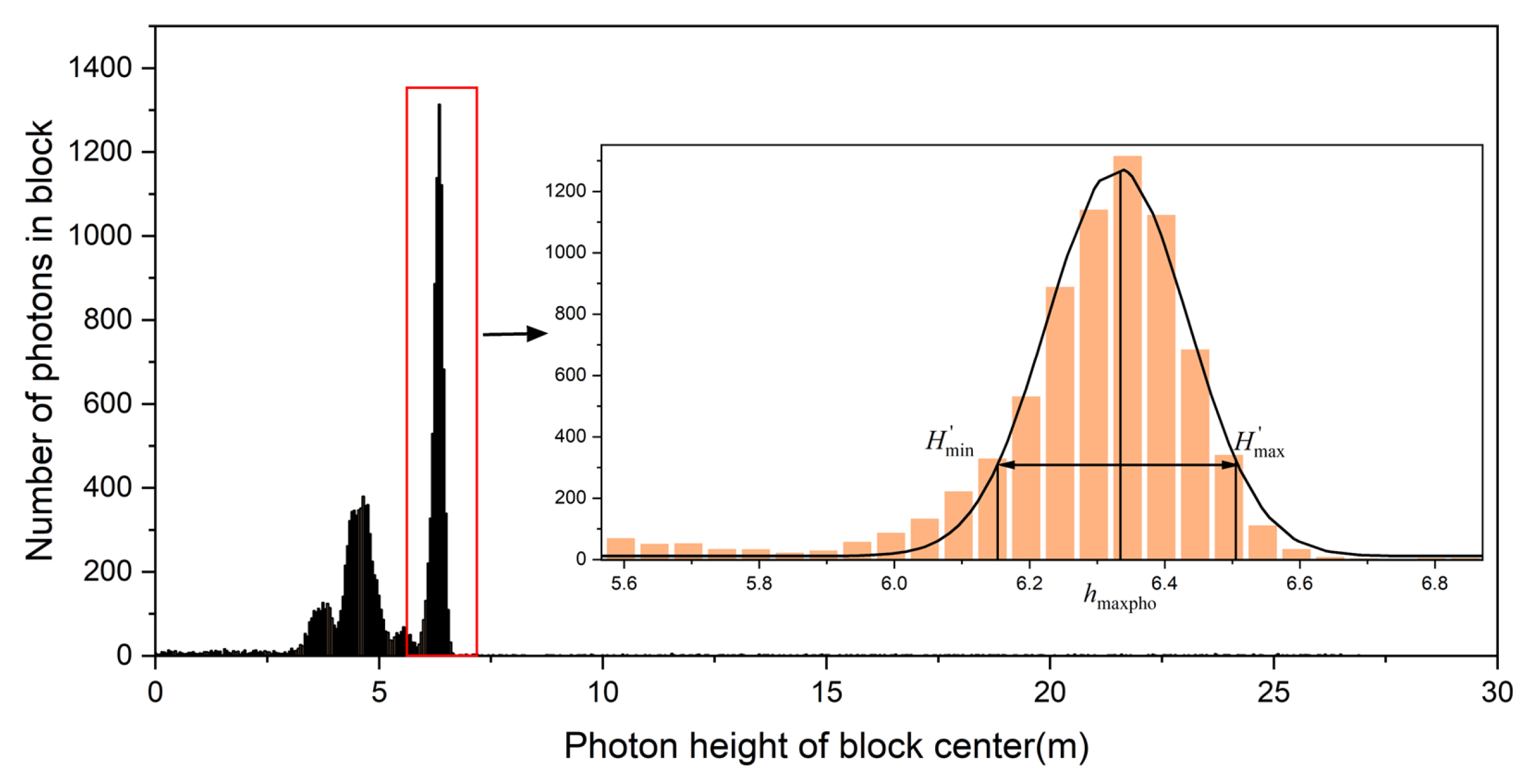
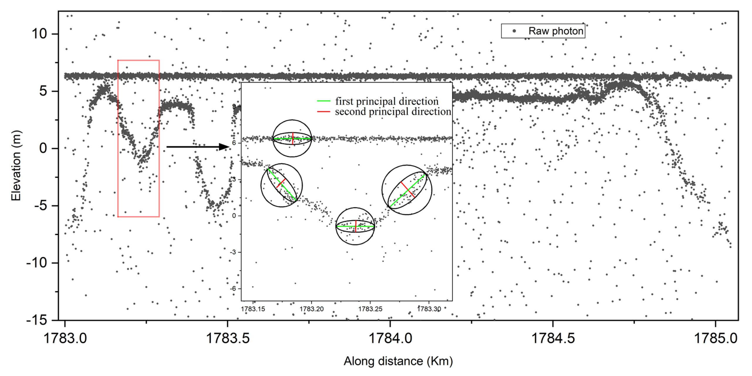
2.1. Extracting Bathymetry Signals

The photon density and distribution in the water column are affected not only by the water depth and environment but also by the different reflectivities of various seafloor sediments and underwater topographies. This is especially true in areas where the underwater topography changes drastically, as the spatial distribution of seafloor photons changes with fluctuations in the topography [19]. In such cases, a horizontal elliptical filter may contain photons on both sides of the crest or trough in the underwater topography. Between the crests and troughs, a horizontal elliptical filter contains fewer seafloor signal photons. Therefore, conventional horizontal elliptical filters do not accurately reflect the photon density information [27]. To achieve efficient and automated segregation and extraction of signal photons originating from both the sea surface and seafloor, the ISDAF model uses an elliptical filter kernel that can adaptively adjust its size and direction according to the water depth and seafloor terrain [12]. Based on the elliptical filter and density threshold, detecting and extracting signal photons from the sea surface and seafloor can be efficiently accomplished [28]. This method includes four key steps: (1) regional photon separation, (2) initial parameter determination, (3) adaptive filter kernel construction, and (4) signal photon extraction [29].

Step 1: Regional photon separation

For the raw point cloud data of the photon-counting LiDAR, using $\Delta h$ as the slice interval in the elevation direction, the original data were divided into t units in the elevation direction, as shown in Figure 2. For the t slice units, the center elevation of each elevation slice $h_t$ can be expressed by counting the number of photon signals in each slice unit $x_t$ in Equation (1):

$$\begin{array}{cc}\hfill h_t=min\left(H_i\right)+{\displaystyle \frac{2t-1}{2}}\Delta h,& \end{array}$$

(1)

where $H_i$ is the elevation of each photon.

The photon height of each block center was taken as the horizontal coordinate, and the number of photons inside the block was taken as a vertical coordinate, as shown in Figure 3. A normal distribution curve was used to fit the relationship between the center elevation of the elevation slice $h_t$ and the number of photon signals in the slice unit, and the fitting relationship $f\left(x\right)$ is obtained as Equation (2):

$$\begin{array}{cccc}& & \hfill f\left(x\right)=x_{\mathrm{maxpho}}exp\left(-{\displaystyle \frac{{(x-h_{\mathrm{maxpho}})}^2}{2{\sigma }^2}}\right),& \end{array}$$

(2)

where $x_{\mathrm{maxpho}}$ represents the number of photons in the elevation slice containing the most photon signals, $h_{\mathrm{maxpho}}$ represents the center elevation of the slice, $\sigma$ denotes the standard deviation observed in a normal distribution, and x is the independent variable of the normal distribution.

Taking $h_{\mathrm{maxpho}}$ as the center and twice the standard deviation as the left and right thresholds, the water surface photon elevation boundary line was defined with Equation (3):

$$\begin{array}{cccc}& & \hfill \left\{\begin{array}{c}{H}_{min}^{\prime }=h_{\mathrm{maxpho}}-2\sigma \hfill \\ H_{max}^{\prime }=h_{\mathrm{maxpho}}+2\sigma ,\hfill \end{array}\right.& \end{array}$$

(3)

where $H_{min}^{\prime }$ represents the minimum elevation of photons on the water surface, and $H_{max}^{\prime }$ denotes the maximum elevation of photons on the water surface.

Taking $H_{min}^{\prime }$ and $H_{max}^{\prime }$ as the boundaries, we obtained the elevation of each photon present on the water surface to form a water surface ($SP$) and an underwater ($WP$) photon set using Equation (4):

$$\begin{array}{cccc}& & \hfill \left\{\begin{array}{c}SP=\{(S{D}_k,S{H}_k)\mid k\in [1,N_{sp}]\}\hfill \\ WP=\{(W{D}_l,W{H}_l)\mid l\in [1,N_{wp}]\},\hfill \end{array}\right.& \end{array}$$

(4)

where $SD$ represents the distance along the track of a photon in the $SP$ set, $SH$ represents the elevation of a photon in the $SP$ set, and $N_{sp}$ is the number of photons in the original dataset that meet the following conditions: $H_{min}^{\prime }<S{H}_k<H_{max}^{\prime }$. $W{D}_l$ represents the distance along the track of a photon in the $WP$ set, $W{H}_l$ represents the elevation of a photon in the $WP$ set, and $N_{wp}$ is the number of photons in the original dataset that satisfy the following conditions: $W{H}_l<H_{min}^{\prime }$.

Step 2: Initial parameter determination

In the SP set along the orbital direction, taking the photon-counting lidar resolution length $\Delta d$ along the orbital direction as the boundary, putting the sea surface photons into q datasets $W{P}_u$ as Equation (5):

$$\begin{array}{cccc}& & \hfill \left\{\begin{array}{c}q={\displaystyle \frac{max\left(S{D}_k\right)-min\left(S{D}_k\right)}{\Delta d}}\hfill \\ W{P}_u=\left(S{D}_u,S{H}_u\right),u\in [1,q].\hfill \end{array}\right.& \end{array}$$

(5)

By counting the maximum difference of photons in the elevation direction $\Delta S{H}_u$ in the q sets, we obtained the average value Ratio_ab, which is the ratio of the major axis to the minor axis of the search ellipse, determined as the length of the semi-minor axis b, which is obtained as $2\sigma$, thereby calculating the length of the semi-major axis a as Equation (6):

$$\begin{array}{cccc}& & \hfill \left\{\begin{array}{c}\Delta S{H}_u=max\left(S{H}_u\right)-min\left(S{H}_u\right)\hfill \\ Ratio\_ab={\displaystyle \frac{{\sum }_{u=1}^q\Delta d/\Delta S{H}_u}{q}}\hfill \\ b=2\ast \sigma \hfill \\ a=b\ast Ratio\_ab\hfill \end{array}\right.& \end{array}$$

(6)

In the SP set, a is the major axis of the search ellipse traversing all data points with this point as the center, and b is the minor axis of the search ellipse used to construct the search area that counts the number of points in the search area $p_v$, $v=1,2,3,\cdots ,N_{sp}$ and calculates the average value of the number of points to obtain the initial minimum number of points (minpts) with Equation (7):

$$\begin{array}{cccc}& & \hfill minpts={\displaystyle \frac{{\sum }_{v=1}^{N_{sp}}{p}_v}{N_{sp}}}.& \end{array}$$

(7)

Step 3: Adaptive filtering kernel construction

Traversing each point in the SP sets, SD_k, SH_k are taken as the center and used to construct a circle with a as the radius. The photons contained within the circle are denoted as the photon set in S_p. Principal component analysis (PCA) is performed based on S_p, and the principal components are calculated to determine the direction of the elliptical filter. The construction of the matrix S is shown in Equation (8), where n represents the number of photons within the circle and m represents the coordinate dimension of each photon; that is, each row represents the location and time information of the photon. Subsequently, the covariance matrix C of matrix S is computed as shown in Equation (9). The centralized matrix S_c is defined in Equation (10) and $\overline{X_1},\overline{X_2},\cdots ,\overline{X_m}$ represent the mean values of different dimensions. The covariance matrix C was diagonalized, and an orthogonal matrix U was determined such that ${\mathbf{U}}^{\mathbf{T}}\mathbf{C}\mathbf{U}=\Lambda$ is satisfied. Therefore, by solving matrix C, the eigenvalue matrix $\Lambda$ and eigenvector matrix U were obtained in Equation (11), where $\lambda$ is the eigenvalue corresponding to the eigenvector u. According to Equation (11), the direction vector u₁ of the principal component is obtained after the PCA transformation. Thus, the angle $\theta$ between the ellipse and the horizontal direction can be determined as shown in Figure 4.

$$\begin{array}{cccc}& & \hfill \mathbf{S}=\left[\begin{array}{cccc}{X}_{11}& X_{12}& \cdots & X_{1m}\\ X_{21}& X_{22}& \cdots & X_{2m}\\ ⋮& ⋮& \ddots & ⋮\\ X_{n1}& X_{n2}& \cdots & X_{nm}\end{array}\right]& \end{array}$$

(8)

$$\begin{array}{cccc}& & \hfill \mathbf{C}={\displaystyle \frac{{\mathbf{S}}_{\mathbf{c}}^{\mathbf{T}}·{\mathbf{S}}_{\mathbf{c}}}{\mathbf{n}-\mathbf{1}}}C\in {\mathbf{R}}^{\mathbf{n}\times m}& \end{array}$$

(9)

$$\begin{array}{cccc}& & \hfill {\mathbf{S}}_{\mathbf{c}}=\left[\begin{array}{cccc}{X}_{11}-\overline{X_1}& X_{12}-\overline{X_2}& \cdots & X_{1m}-\overline{X_m}\\ X_{21}-\overline{X_1}& X_{22}-\overline{X_2}& \cdots & X_{2m}-\overline{X_m}\\ ⋮& ⋮& \ddots & ⋮\\ X_{n1}-\overline{X_1}& X_{n2}-\overline{X_2}& \cdots & X_{nm}-\overline{X_m}\end{array}\right]& \end{array}$$

(10)

$$\mathbf{C}=\mathbf{U}\Lambda {\mathbf{U}}^{\mathbf{T}}=[u_1,\cdots u_n]·\left[\begin{array}{ccc}{\lambda }_1& & \\ & \ddots & \\ & & {\lambda }_n\end{array}\right]·\left[\begin{array}{c}{u}_1^T\\ ⋮\\ u_n^T\end{array}\right]=\sum _{i=1}^n{\lambda }_i{u}_i{u}_i^T.$$

(11)

In the WP set, centered on the point (WD_l, WH_l), the ellipse semi-major axis a_l, semi-minor axis b_l, and minimum point threshold minpts_l are all related to the sea surface photon filtering ellipse major axis, minor axis, minimum point threshold initial value, and correlation coefficient a_f, which was determined by the relationship between the change in seafloor photons and water depth as Equation (12):

$$\begin{array}{cccc}& & \hfill \left\{\begin{array}{c}{a}_l=b_l\times Ratio\_ab\hfill \\ b_l=b\times \left(1+a_f\times abs\left(W{H}_l-H_{min}^{\prime }\right)\right),l\in [1,N_{wp}]\hfill \\ minpt{s}_l=minpts\times \left(1-a_f\times abs\left(W{H}_l-H_{min}^{\prime }\right)\right).\hfill \end{array}\right.& \end{array}$$

(12)

Step 4: Signal photons detection

For each point in the SP set, we used the point (SD_k, SH_k) as the center to calculate the angle ${\theta }_k$ by PCA transformation, and a and b as the semi-major and semi-minor axes of the elliptical search area, respectively; to determine whether other points (SD_k, SH_k) in the SP set were located in the search area as (Equations (13) and (14)). When $dis{s}_x<1$, the point (SD_k, SH_k) is located in the elliptical search area centered on (SD_k, SH_k) and the algorithm counts all the signal points in the search area. When $dis{s}_x>minpts$, it indicates (SD_k, SH_k) as a signal point of the sea surface; otherwise, it is a noise point [30].

$$\begin{array}{cccc}& & \hfill dis{s}_x={\displaystyle \frac{x_s^2}{a^2}}+{\displaystyle \frac{y_s^2}{b^2}}& \end{array}$$

(13)

$$\begin{array}{cccc}& & \hfill \left\{\begin{array}{c}{x}_s=\left(S{D}_x-S{D}_k\right)\times sin{\theta }_k+\left(S{H}_x-S{H}_k\right)\times cos{\theta }_k\hfill \\ y_s=\left(S{D}_x-S{D}_k\right)\times sin{\theta }_k-\left(S{H}_x-S{H}_k\right)\times cos{\theta }_k\hfill \end{array}\right..& \end{array}$$

(14)

Traversing each point in the WP set, a circle with radius a_l centered on point $(W{D}_l,W{H}_l)$ is constructed by calculating the angle ${\theta }_l$ by PCA transformation. Then, a_l and b_l were used as the semi-major axis and semi-minor axis of the ellipse to determine whether the other points (WD_x, WH_x) in the WP set are located in the ellipse search area. With this processing of the WP set, the noise above the seafloor signal photons was almost completely removed, while the noise below the seafloor signal photons was still present. Next, a multi-scale statistical method is used for the remaining photon set RP to extract seafloor signal photons. First, the photon set RP was segmented with the same number of photon points n along the LiDAR track. The photons in each segment were then sorted in descending order by elevation. We removed the first 5% and the last 35% of the photons, taking the middle 60% as the seafloor signal photons. The different values of n have a small effect on the seafloor signal photon extraction results, especially in places where the seafloor topography is relatively variable. Therefore, three n values—20, 30, and 50—were used for extracting seafloor signal photons, and then the three sets of results were superimposed to obtain the final seafloor signal photons as shown in Figure 5.

2.2. Refraction Correction for Seafloor Photons

To accurately determine the water depth along the ICESat-2 tracks, it was necessary to correct the ATL03 data for refraction. In reality, the sea surface constantly fluctuates, and this has an impact on the refraction effect within the water column. Therefore, considering the influence of the water column, a precise refraction correction was applied to every seafloor signal photon using PWCP. The signal photons on the sea surface exhibit a high concentration, offering a favorable condition for accurately reconstructing the local sea wave profile using PWCP as Equation (15), where a_j, b_j, c_j, and d_j are the coefficients of the cubic polynomial, which are used to describe the local sea wave profile, j is the number of seafloor photons, and the weight function is represented by w, which adjusts the influence of each photon based on its distance from the reference point.

$$\begin{array}{cccc}& & \hfill \left\{\begin{array}{c}z\left(x\right)=a_j{x}^3+b_j{x}^2+c_{j}x+d_j\hfill \\ w={\displaystyle \frac{1}{∥x-x_{p^{\prime }}∥}};w={\displaystyle \frac{1}{{(x-x_{p^{\prime }})}^2}}.\hfill \end{array}\right.& \end{array}$$

(15)

Assuming that six sea surface photons were used in the PWCP model, the cubic polynomial parameters for the seafloor photon p were solved using the least squares method. Equation (16) represents the error equation, and the coefficient matrices A, value matrix L, and unknown vector matrix X are shown in Equation (17):

$$v_i=a_j{x}_i^3+b_j{x}_i^2+c_j{x}_i+d_j-z\left(x_i\right),(i=1,2,\cdots ,6)$$

(16)

$$\begin{array}{cc}\hfill \mathbf{A}=\left[\begin{array}{cccc}1& x_1& x_1^2& x_1^3\\ 1& x_2& x_2^2& x_2^3\\ ⋮& ⋮& ⋮& ⋮\\ 1& x_6& x_6^2& x_6^3\end{array}\right] \mathbf{L}=\left[\begin{array}{c}{l}_1\\ l_2\\ ⋮\\ l_6\end{array}\right] \mathbf{X}=\left[\begin{array}{c}{a}_j\\ b_j\\ c_j\\ d_j\end{array}\right]& \end{array}$$

(17)

Based on the weight equation, weights $w_1,w_2,\cdots$ , and $w_6$ for the sea surface photons were calculated, followed by the construction of the weight matrix W. In accordance with the principles of the least-squares method, the coefficient matrix N for solving the normal equation, accompanied by its corresponding free vector U, was created and presented as follows: The parameters in the polynomial for seafloor photon q were solved and obtained by matrix X, as represented in Equation (18) and Equation (19), respectively.

$$\begin{array}{cc}\hfill \mathbf{N}={\mathbf{A}}^{\mathbf{T}}\mathbf{WA}=\left[\begin{array}{cccc}{w}_1+\cdots +w_6& w_1{x}_1+\cdots +w_6{x}_6& \cdots & w_1{x}_1^3+\cdots +w_6{x}_6^3\\ w_1{x}_1+\cdots +w_6{x}_6& w_1{x}_1^2+\cdots +w_6{x}_6^2& \cdots & w_1{x}_1^4+\cdots +w_6{x}_6^4\\ w_1{x}_1^2+\cdots +w_6{x}_6^2& w_1{x}_1^3+\cdots +w_6{x}_6^3& \cdots & w_1{x}_1^5+\cdots +w_6{x}_6^5\\ w_1{x}_1^3+\cdots +w_6{x}_6^3& w_1{x}_1^4+\cdots +w_6{x}_6^4& \cdots & w_1{x}_1^6+\cdots +w_6{x}_6^6\end{array}\right]& \end{array}$$

(18)

$$\begin{array}{cc}\hfill \mathbf{U}=\left[\begin{array}{c}{l}_1{w}_1+l_2{w}_2+\cdots +l_6{w}_6\\ l_1{x}_1{w}_1+l_2{x}_2{w}_2+\cdots +l_6{x}_6{w}_6\\ l_1{x}_1^2{w}_1+l_2{x}_2^2{w}_2+\cdots +l_6{x}_6^2{w}_6\\ l_1{x}_1^3{w}_1+l_2{x}_2^3{w}_2+\cdots +l_6{x}_6^3{w}_6\end{array}\right]\mathbf{X}=\left[\begin{array}{c}{a}_j\\ b_j\\ c_j\\ d_j\end{array}\right]={\mathbf{N}}^{-1}·\mathbf{U}& \end{array}$$

(19)

Subsequently, the local sea wave profile for the seafloor photon p was determined using the solved polynomial parameters. Finally, a precise calculation of the coordinates of the intersection point q was achieved by utilizing the local sea wave profile and the constructed spatial line of photon p.

To determine the actual coordinates of seafloor photons, we performed photon path tracing based on the slope of the sea surface and considered diverse pointing angles of the laser beam. By analyzing the intersection points where laser beams meet the sea surface, we observed fluctuations in incident and refraction angles owing to variations in the slope of the sea surface as shown in Figure 6.

In various situations where water refraction is involved, the angles of inclination on the surface of the sea can be classified into three distinct ranges: ${\phi }_x^q\in (0,{\theta }_x)$, ${\phi }_x^q\in ({\theta }_x,{\theta }_x+{90}^{°})$, and ${\phi }_x^q\in (\theta +{90}^{°},{180}^{°})$. The laser beam’s pointing angle (${\theta }_x$) can either be ≥zero or ≤zero. Consequently, by considering the spatial geometry of the incident angle, refraction angle, and transmission path of photons through the water column toward the seafloor, we expressed displacement in terms of ${\epsilon }_x$ for the along-track direction, ${\epsilon }_y$ for the cross-track direction, and ${\epsilon }_z$ for the elevation direction. The displacements are formulated as Equations (20)–(22).

$$\left[\begin{array}{c}{\epsilon }_x\\ {\epsilon }_y\\ {\epsilon }_z\end{array}\right]=\left[\begin{array}{c}{R}_x·sin({\phi }_x^q+{\beta }_x)-L_x·sin{\theta }_x\hfill \\ L_y·sin{\theta }_y-R_y·sin({\theta }_y-{\beta }_y)\hfill \\ L_x·cos{\theta }_x-R_x·cos({\phi }_x^q+{\beta }_x)\hfill \end{array}\right]=L_x·\left[\begin{array}{c}sin({\phi }_x^q+{\beta }_x)/n_w-sin{\theta }_x\hfill \\ {\displaystyle \frac{cos{\theta }_x}{cos{\theta }_y}}·\left[sin{\theta }_y-sin({\theta }_y-{\beta }_y)/n_w\right]\hfill \\ cos{\theta }_x-cos({\phi }_x^q+{\beta }_x)/n_w\hfill \end{array}\right],{\phi }_x^q\in (0,{\theta }_x)$$

(20)

$$\left[\begin{array}{c}{\epsilon }_x\\ {\epsilon }_y\\ {\epsilon }_z\end{array}\right]=\left[\begin{array}{c}{R}_x·sin({\phi }_x^q-{\beta }_x)-L_x·sin{\theta }_x\hfill \\ L_y·sin{\theta }_y-R_y·sin({\theta }_y-{\beta }_y)\hfill \\ L_x·cos{\theta }_x-R_x·cos({\phi }_x^q-{\beta }_x)\hfill \end{array}\right]=L_x·\left[\begin{array}{c}sin({\phi }_x^q-{\beta }_x)/n_w-sin{\theta }_x\hfill \\ {\displaystyle \frac{cos{\theta }_x}{cos{\theta }_y}}·\left[sin{\theta }_y-sin({\theta }_y-{\beta }_y)/n_w\right]\hfill \\ cos{\theta }_x-cos({\phi }_x^q-{\beta }_x)/n_w\hfill \end{array}\right],{\phi }_x^q\in ({\theta }_x,{\theta }_x+{90}^{°})$$

(21)

$$\left[\begin{array}{c}{\epsilon }_x\\ {\epsilon }_y\\ {\epsilon }_z\end{array}\right]=\left[\begin{array}{c}{R}_x·sin({\phi }_x^q+{\beta }_x-{180}^{°})-L_x·sin{\theta }_x\hfill \\ L_y·sin{\theta }_y-R_y·sin({\theta }_y-{\beta }_y)\hfill \\ L_x·cos{\theta }_x-R_x·cos({180}^{°}-{\phi }_x^q-{\beta }_x)\hfill \end{array}\right]=L_x·\left[\begin{array}{c}-sin({\phi }_x^q+{\beta }_x)/n_w-sin{\theta }_x\hfill \\ {\displaystyle \frac{cos{\theta }_x}{cos{\theta }_y}}·\left[sin{\theta }_y-sin({\theta }_y-{\beta }_y)/n_w\right]\hfill \\ cos{\theta }_x+cos({\phi }_x^q+{\beta }_x)/n_w\hfill \end{array}\right],{\phi }_x^q\in (\theta +{90}^{°},{180}^{°}).$$

(22)

3. Study Area and Dataset

3.1. Study Area

Our study area included four islands and reefs: Vieques Island (${18}^{°}{06}^{\prime }{35}^{″}$N, ${65}^{°}{25}^{\prime }{17}^{″}$W), Lingyang Reef (${16}^{°}{27}^{\prime }{35}^{″}$N, ${112}^{°}{31}^{\prime }{17}^{″}$E), Langhua Reef (${16}^{°}{32}^{\prime }{1}^{″}$N, ${112}^{°}{31}^{\prime }{17}^{″}$E) and Huaguang Reef (${16}^{°}{12}^{\prime }{52}^{″}$N, ${111}^{°}{40}^{\prime }{22}^{″}$E). Vieques Island is the second-largest island in the Puerto Rico archipelago. The other three reefs are situated in the Xisha Islands of the South China Sea. These islands and reefs have different seafloor terrains, are less affected by human activities, and have well-protected natural environments. Therefore, the water quality around the research area was sufficiently clear and suitable for the laser bathymetry experiments. Figure 7 shows images of the study area, with their locations marked with different colored stars.

3.2. ATLAS ATL03 Dataset

Since 14 October 2018, ICESat-2 has been actively gathering data and offers various data products, including the publicly accessible Global Geolocated Photon Level 2A dataset, called ATL03, available on the National Snow and Ice Data Center website. To evaluate the performance of the proposed method, 7 ATL03 datasets were used, and the photon information of eight ground tracks was obtained. The eight ground tracks are represented by dashed lines in Figure 7. In general, the seafloor terrain of Vieques Island and Lingyang Reef is relatively flat, whereas that of Langhua Reef and Huaguang Reef varies greatly.

Table 1. Distribution information of ATLAS ATL03 datasets in the study sites.

Island(s) in Transit	ATLAS Dataset	Time (UTC)	Track ID	Beam	Geodetic Coordinates (Longitude, Latitude)
Vieques Island	20220319 20210919	21:05 04:51	1337	GT2L GT1R	18°4′26″N, 66°30′4″W–18°5′38″N, 66°30′11″W 18°4′31″N, 66°31′42″W–18°5′31″N, 66°31′49″W
Lingyang Reef	20210818 20210818	18:30 18:30	857	GT3L GT3R	16°29′33″N, 111°34′42″E–16°27′1″N, 111°34′27″E 16°29′28″N, 111°34′40″E–16°27′0″N, 111°34′25″E
Langhua Reef	20190417 20200715	23:07 01:26	301	GT2L GT3L	16°2′11″N, 112°27′22″E–16°3′18″N, 112°27′15″E 16°1′14″N, 112°31′4″E–16°2′12″N, 112°30′58″E
Huaguang Reef	20200719	01:19	362	GT1L	16°11′45″N, 111°39′40″E–16°12′39″N, 111°39′35″E
	20190222	13:51	857	GT2L	16°14′7″N, 111°36′57″E–16°13′2″N, 111°36′51″E

shows the detailed distribution information of the eight ground-track datasets.

3.3. Reference Data

The Riegl VQ-880-G II sensor was utilized by Leading Edge Geomatics to collect bathymetric reference data from Vieques Island. The data acquisition period spanned from 20 January 2019 to 2 June 2019. Achieving a vertical accuracy of 8.6 cm and a horizontal accuracy of 69.6 cm was accomplished during this process. In the Lingyang Reef area, the reference data of the in situ water depth were obtained by the Mapper5000 ALB system on 16 June 2018, and 27 September 2017, respectively [31]. The Mapper5000 is designed to achieve a bathymetric accuracy of up to 0.23 m. We have not yet obtained the in situ data of Langhua Reef and Huaguang Reef; therefore, we will only show the experimental results of these areas and make a comparative analysis.

The local water level may undergo fluctuations due to tidal influences. Hence, we utilized the NAO.99b tide model [32] to analyze variations in tidal heights during the ICESat-2 trajectory acquisition period and then compare them with in situ water depth measurements, aiming to eliminate the impact of tides.

4. Experimental Results

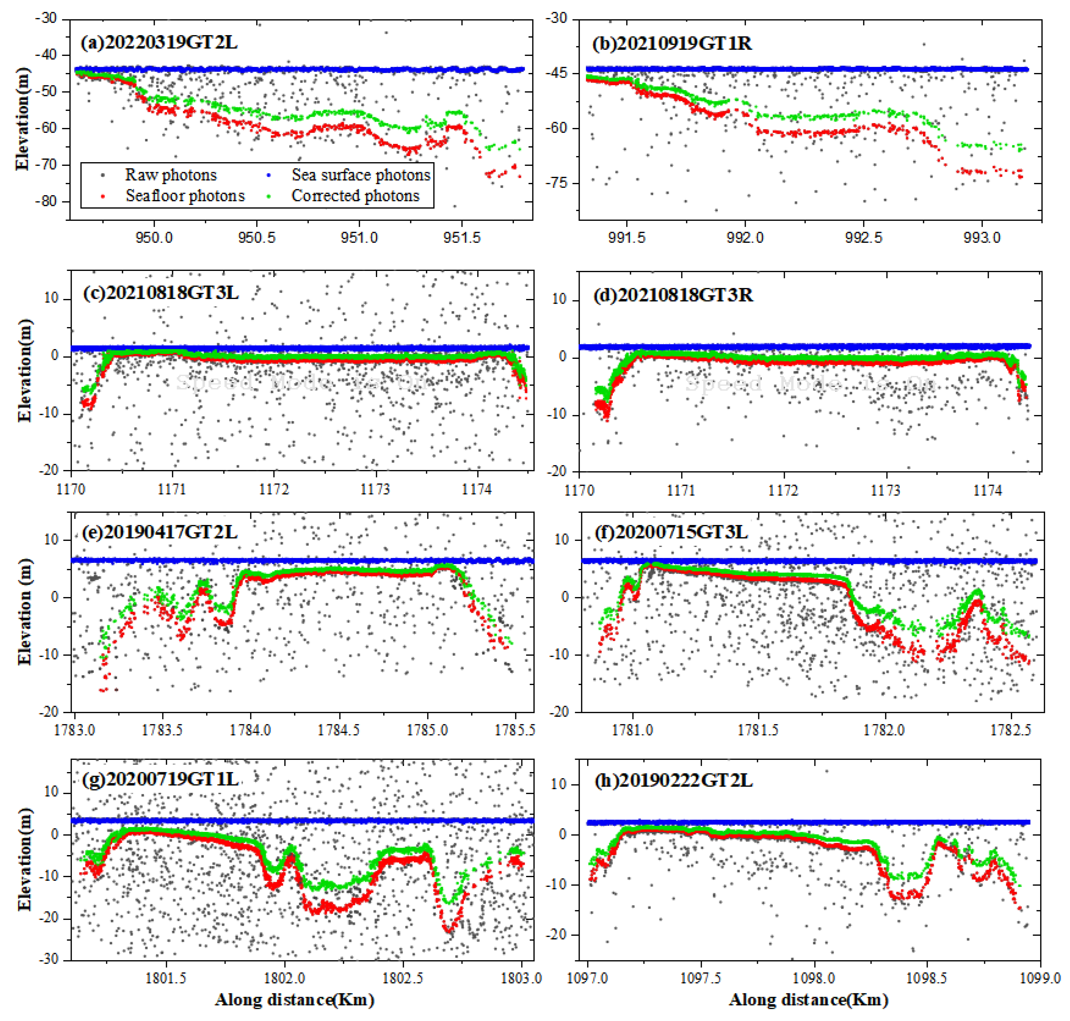
4.1. Signal Photon Detection Results

To assess the precision and generalization ability of the proposed method, a series of experiments were performed utilizing eight photon datasets within the study area. The ISDAF was used to automatically extract signal photons of different regions and types by adaptively determining the elliptic filter parameters. As depicted in Figure 8, the ISDAF has the capability to autonomously distinguish photons above the sea surface, at the sea surface, and below the sea surface in different regional datasets and accurately extract different types of signal photons. Datasets 20220319GT2L, 20210919GT1R, 20210818GT3R, and 20190222GT2L were collected at night and were less affected by sunlight. Therefore, there were fewer noisy photons in these three datasets, and the overall photon density was lower than that of the other datasets. Usually, a higher-density photon dataset is mixed with more noise photons, which increases the difficulty of extracting various signal photons, especially seafloor signal photons [33]. Compared with surface signal photons, seafloor signal photons are more likely to have some discontinuities, especially when the water depth is relatively deep and the bottom terrain varies significantly, as shown in Figure 8e–h. As the water depth increases, the water body has a greater effect on the attenuation of laser energy, and the number of signal photons reaching the bottom of the water decreases, which also increases the difficulty in extracting signal photons [34,35,36]. The comprehensive experimental results indicated that, regardless of changes in seafloor terrain, the ISDAF accurately extracted seafloor signal photons.

4.2. Refraction Correction Results

Because there is a refraction effect when the laser is transmitted in a water column, the measurement accuracy of the water depth is affected [37]. Therefore, it is necessary to correct the coordinates of the seafloor photons. The correction results for different datasets based on the refraction correction method for seafloor photons are shown in Figure 9. After applying refraction correction, the coordinates of the seafloor signal photons exhibited different degrees of upward shift, and the water depth measured at the corresponding position decreased accordingly.

Furthermore, the bathymetric results of the 8 photon datasets after correction indicated that the maximum water depth that could be detected within the study area was 21.86 m in the 20220319GT2L dataset, as shown in

Table 2. Results of the minimum and maximum bathymetric measurements obtained from the eight datasets before and after refraction correction, along with their corresponding differences.

ATLAS ATL03 Dataset	Depth Before Correction (m)		Depth After Correction (m)		Difference (m)
	Min	Max	Min	Max	Min	Max
20220319GT2L	0.75	29.30	0.57	21.86	0.18	7.44
20210919GT1R	2.84	29.13	2.12	21.79	0.72	7.34
20210818GT3L	0.46	9.78	0.34	7.33	0.12	2.45
20210818GT3R	1.24	11.83	0.91	8.84	0.33	2.99
20190417GT2L	0.24	14.77	0.15	11.01	0.09	3.76
20200715GT3L	0.69	17.34	0.49	12.95	0.20	4.39
20200719GT1L	0.64	18.78	0.45	14.02	0.19	4.76
20190222GT2L	0.97	15.85	0.71	11.81	0.26	4.04

. If refraction correction is not performed, the bathymetric error can reach 7.44 m. The minimum water depth that could be detected was 0.15 m in the 20190417GT2L dataset and 0.24 m before refraction correction, which was in the nearshore area. The minimum water depth difference before and after refraction correction ranged from 0.09 to 0.72 m, and the refraction offset was at the centimeter or decimeter level. The maximum water depth difference ranged from 2.45 to 7.44 m, and the refraction offsets reached the meter level. These results indicated that the increase in water depth directly correlates with a proportional rise in bathymetric error resulting from the refraction effect of the water column. Therefore, it is necessary to correct the change in photon coordinates caused by water column refraction when performing bathymetry based on the ATLAS ATL03 dataset.

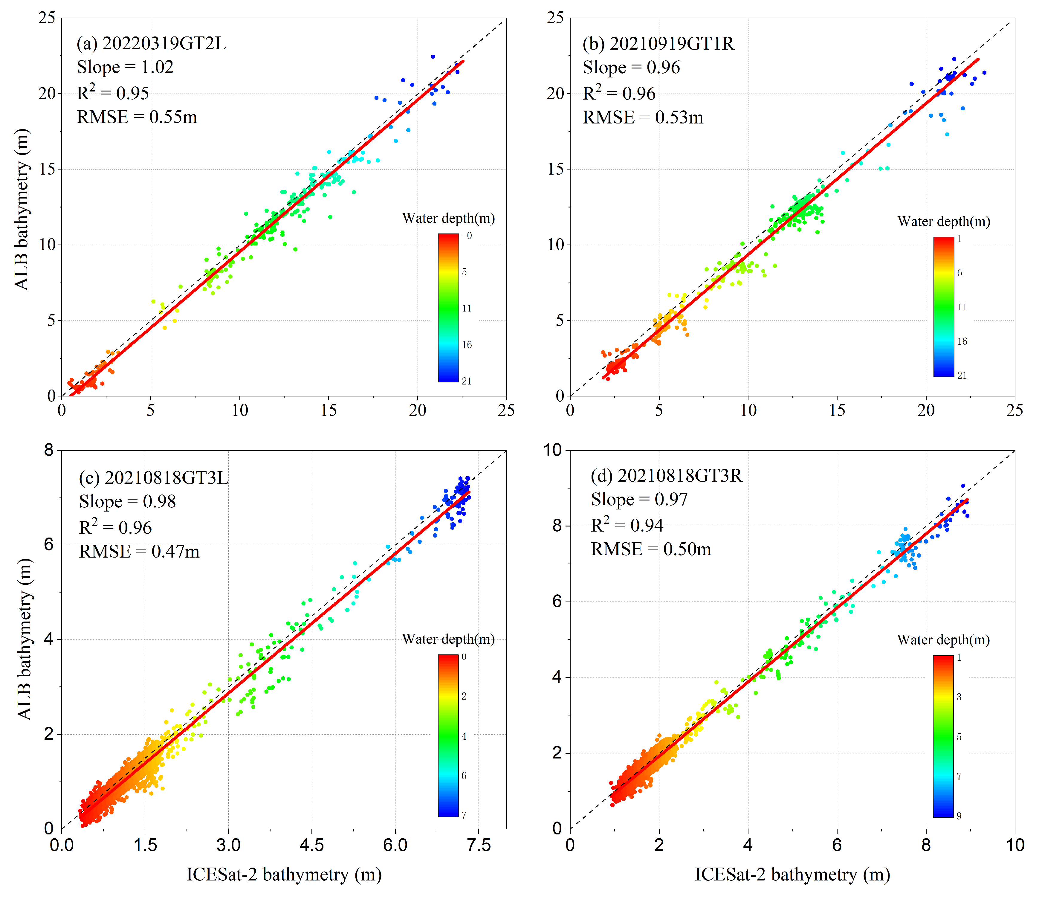
4.3. Bathymetric Accuracy and Validation

To verify the precision of ICESat-2 data in measuring bathymetry using the ISDAF method, we calculated the bathymetric results for each dataset after refraction correction, using the four datasets obtained from Vieques Island and Lingyang Reef. The slope, R², and RMSE were calculated and compared with the verification data as shown in Figure 10 and

Table 3. Bathymetry accuracy verification results of the ICESat-2 dataset before and after refraction correction.

ATLAS ATL03 Dataset	Before Refraction Correction			After Refraction Correction
	Slope	R2	RMSE (m)	Slope	R2	RMSE (m)
20220319GT2L	1.27	0.92	1.33	1.02	0.95	0.55
20210919GT1R	1.24	0.93	1.19	0.96	0.96	0.53
20210818GT3L	1.23	0.95	1.15	0.98	0.96	0.47
20210818GT3R	1.24	0.93	1.18	0.97	0.94	0.50
Overall	1.36	0.94	1.20	1.07	0.95	0.53

. There was a strong correlation between the ICESat-2 photon bathymetry results obtained by ISDAF and the ALB verification data, with all slopes close to 1. R² was greater than or equal to 0.94, and the largest R² was 0.96, which was obtained from dataset 20210919GT1R and dataset 20210818GT3L. The RMSE on all datasets was less than 0.6 m, with the smallest RMSE of 0.47 m observed in dataset 20210818GT3L. The overall R² of the four datasets was as high as 0.95, the slope was 1.07, and the RMSE was 0.53 m. These findings suggested that bathymetric results derived from the ISDAF were highly accurate and reliable.

To analyze the impact of water column refraction on bathymetry results, the correlations between ICESat-2 bathymetry results without refraction correction and the ALB verification data were compared in Table 3. Compared to the verification results before refraction correction, the corrected slope of each dataset was reduced by approximately 0.3, and they were all close to 1. Owing to the laser’s small incident angle, the refraction correction process can be approximated as a linear decrease in the water depth before correction; therefore, the change in R² before and after refraction correction was small and within 0.03. After correction, the RMSE decreased significantly from the meter level to the decimeter level, indicating that bathymetry accuracy was significantly improved. After merging the four datasets, the overall slope of the verification model was reduced from 1.36 to 1.07, the RMSE increased from 1.20 m to 0.53 m, and R² increased from 0.94 to 0.95.

5. Analysis and Discussion

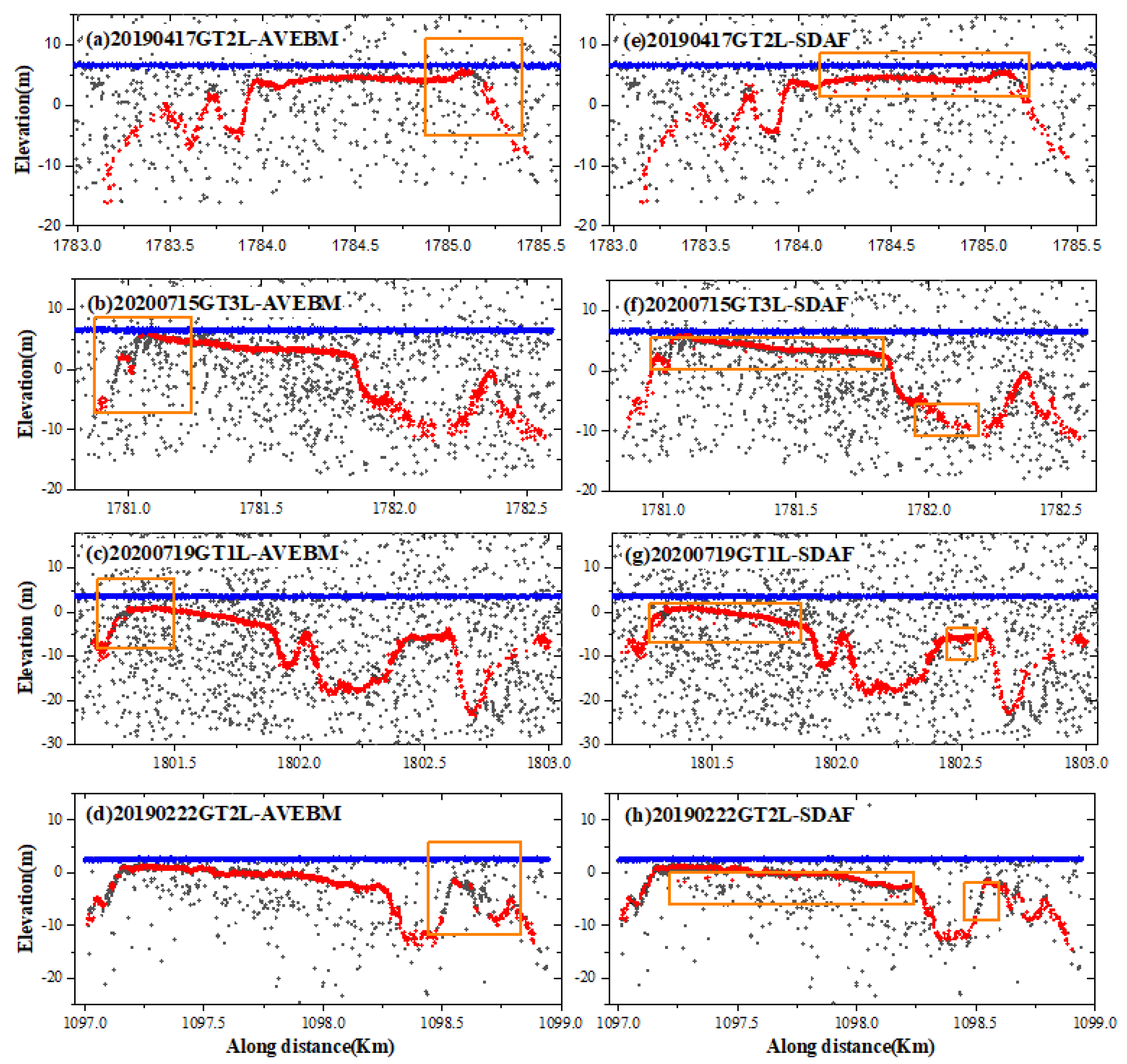
5.1. Detection Capability of Our Method

The number of different types of photons in each dataset and their respective proportions were used to analyze the signal photon detection capability of ISDAF, as shown in

Table 4. The number and proportion of different types of photons in each dataset after using ISDAF.

ATLAS ATL03 Dataset	Total Number of Photons	Number and Proportion of Sea Surface Photons	Number and Proportion of Seafloor Photons	Number and Proportion of Noise Photons
20220319GT2L	4686	3296 (70.34%)	519 (11.08%)	871 (18.58%)
20210919GT1R	10,704	9732 (90.92%)	548 (5.12%)	424 (3.96%)
20210818GT3L	26,400	12,602 (47.73%)	10,040 (38.03%)	3758 (14.24%)
20210818GT3R	21,675	10,477 (48.34%)	9421 (43.46%)	1777 (8.20%)
20190417GT2L	16,657	7141 (42.87%)	7023 (42.16%)	2493 (14.97%)
20200715GT3L	9569	4999 (52.24%)	2502 (26.15%)	2068 (21.61%)
20200719GT1L	5159	1960 (37.99%)	1462 (28.34%)	1737 (33.67%)
20190222GT2L	7465	3827 (51.27%)	2635 (35.29%)	1003 (13.44%)

. Due to differences in the water environment, light environment, and data span during the acquisition of the eight datasets, the total number of photons in each dataset varied. Among them, dataset 20210818GT3L from Lingyang Reef had the highest number of photons (26,400), and the dataset span was approximately 4.50 km. Dataset 20220319GT2L from Vieques Island had the lowest number of photons (4686), and the dataset spanned approximately 2.20 km. When the laser pulse emitted by the ATLAS transmitter traverses through the atmosphere and reaches the sea surface, most of the photons return to the receiver because of reflection from the sea surface [38]. Therefore, there is a higher proportion of photons originating from the sea surface compared to those from the seafloor and background noise. Among all datasets examined, dataset 20210919GT1R in Vieques Island exhibited the highest percentage of photons reflecting off the sea surface at 90.92%. After the photons penetrate the sea surface, they are scattered in the water body and treated as noise photons, while the photons that reach the bottom are detected and treated as seafloor signal photons. In general, the proportion of signal photons at the seafloor was greater than that of noise photons. However, because sunlight is also reflected to the laser receiver, the proportion of noise photons may be larger than that of seafloor signal photons, especially when sunlight is very strong. For example, for the dataset 20220319GT2L, the proportion of water bottom photons was 11.08% and the proportion of noise photons was 18.58%. As datasets 20210919GT1R, 20210818GT3R, and 20190222GT2L were acquired at night and were less affected by ambient light, the proportion of noisy photons was less than 14%.

To further verify the advantages of ISDAF using the four datasets with large fluctuations in seafloor terrain acquired at the Langhua and Huaguang reefs, we compared it with two filtering methods: AVEBM [25] and SDAF [26]. The number of different types of photons extracted after using AVEBM and SDAF is shown in

Table 5. The number and proportion of different types of photons in each dataset after using AVEBM.

ATLAS ATL03 Dataset	Total Number of Photons	Number and Proportion of Sea Surface Photons	Number and Proportion of Seafloor Photons	Number and Proportion of Noise Photons
20190417GT2L	16,657	7090 (42.56%)	6901 (41.43%)	2666 (16.01%)
20200715GT3L	9569	4932 (51.54%)	2419 (25.28%)	2218 (23.18%)
20200719GT1L	5159	1888 (36.60%)	1406 (27.25%)	1865 (36.15%)
20190222GT2L	7465	3744 (50.15%)	2553 (34.20%)	1168 (15.65%)

and

Table 6. The number and proportion of different types of photons in each dataset after using SDAF.

ATLAS ATL03 Dataset	Total Number of Photons	Number and Proportion of Sea Surface Photons	Number and Proportion of Seafloor Photons	Number and Proportion of Noise Photons
20190417GT2L	16,657	7180 (43.11%)	7044 (42.29%)	2433 (14.60%)
20200715GT3L	9569	5028 (52.54%)	2537 (26.51%)	2004 (20.95%)
20200719GT1L	5159	1978 (38.34%)	1487 (28.82%)	1694 (32.84%)
20190222GT2L	7465	3844 (51.49%)	2628 (35.20%)	993 (13.31%)

, respectively. The signal photons extraction results of the two methods are shown in Figure 11. Compared with ISDAF, we found that the sea surface and seafloor signal photons extracted using the AVEBM were reduced to varying degrees, and the proportion of noise photons increased in Table 5. Among them, the sea surface signal photons and seafloor signal photons extracted from datasets 20200719GT1L and 20200715GT3L accounted for the smallest proportions (36.60% and 25.28%, respectively), which were reduced by 1.39% and 0.87%, respectively, according to Table 4 and Table 5. The remaining noise photons in dataset 20200719GT1L accounted for the highest proportion (36.15%), which was an increase of 2.48% when compared with the results from the ISDAF analysis. Meanwhile, as shown in Table 5 and Table 6, SDAF exhibits a performance opposite to that of AVEBM. Specifically, SDAF extracts a greater number of sea surface photons and seafloor signal photons. Notably, the proportion of sea surface signal photons extracted by dataset 20200715GT3L reached the highest at 52.54%, whereas the proportion of seafloor signal photons extracted by dataset 20190417GT2L was the highest, accounting for 42.29%.

According to the comparison between Figure 10 and Figure 11, it is evident that the extraction performance of the three methods for photons of sea surface signals is relatively effective. Because of the relatively high concentration of photons present on the surface of water, their extraction becomes more feasible. Compared with AVEBM, both SDAF and ISDAF have better signal photon extraction effects in areas with large seafloor terrain and extract more seafloor signal photons. ISDAF extracted almost all the signal photons in the steep terrain areas, while SDAF performed slightly less well and introduced noise in the gentle areas, as shown in the orange rectangular box in Figure 11. It is very likely that the SDAF rotates the ellipse within a 10-degree interval and does not accurately reflect the direction of the ellipse in this area. Overall, the ISDAF demonstrated better adaptive capabilities and accurately extracted lower-density seafloor signal photons without introducing noise, even in high water depths and when the seafloor terrain changed significantly.

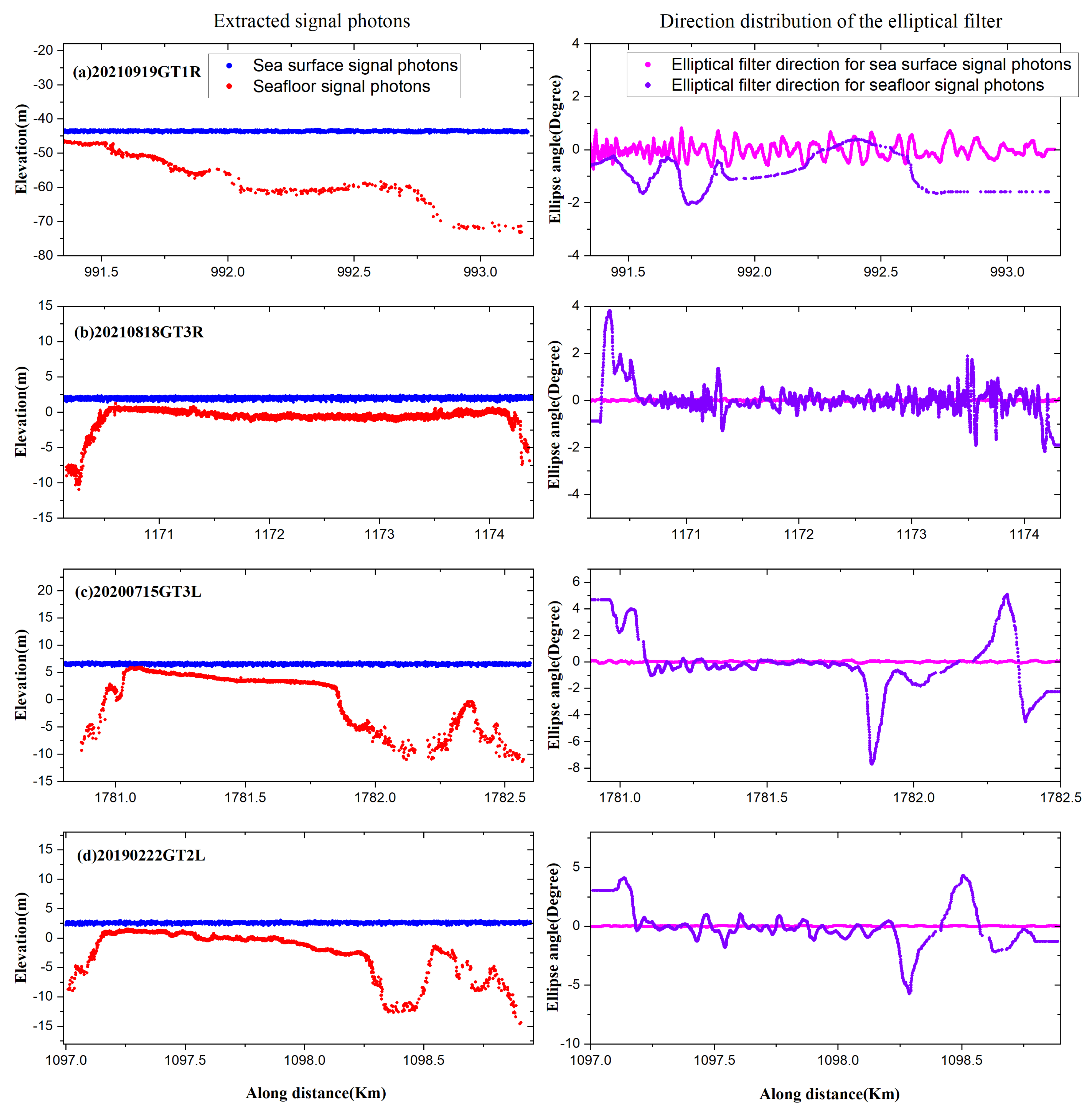
5.2. Directional Adaptability of Ellipses in ISDAF

To better evaluate the performance of ISDAF, we selected four datasets to count the direction distribution of the elliptical filter built around the extracted signal photons in Figure 12. The angles of the ellipses on the sea surface were all distributed near 0 because the sea surface was relatively smooth, and most of the photons were distributed along the track. In the far shore area, the photons on the sea surface also exhibited certain fluctuations [26]. Therefore, the angles of the ellipses on the sea surface were more evident. In Figure 12a,b, the seafloor terrain was relatively gentle; therefore, the angle distribution range was relatively small, especially in the middle area of Figure 12b. As shown in Figure 12c,d, the seafloor terrain changed drastically; therefore, the angle range of the seafloor ellipse was also relatively large. The seafloor ellipse in dataset 20200715GT3L had the largest angle range and the largest ellipse direction, which exceeded ${12}^{°}$. In general, the directions of the ellipses constructed from the sea surface and seafloor signal photons were consistent with the distribution characteristics of the corresponding signal photons.

We further assessed the statistics on the maximum and minimum values and their differences in the angle of the elliptical filter constructed using signal photons from both the sea surface and the seafloor across the four datasets in

Table 7. Statistical results of elliptical direction distribution centered on sea surface and seafloor signal photons.

ATLAS ATL03 Dataset	Angle of the Ellipse Centered on the Water Surface Photon (Degree)			Angle of the Ellipse Centered on the Seafloor Photon (Degree)
	Minimum	Maximum	Difference	Minimum	Maximum	Difference
20210919GT1R	−0.62	0.58	1.20	−2.07	0.39	2.46
20210818GT3R	−0.10	0.09	0.19	−2.17	3.82	5.98
20200715GT3L	−0.19	0.23	0.41	−7.68	5.08	12.76
20190222GT2L	−0.08	0.08	0.16	−5.74	4.31	10.05

. The angle sizes of the sea surface ellipses were close to 0, and the smallest angle was observed in the 20210919GT1R dataset, which was $-0.62°$. The largest angle was observed in the same dataset ($0.58°$), which also exhibited the largest difference in angle ($1.20°$), indicating that the sea surface of this dataset fluctuated significantly. The smallest difference was observed in dataset 20190222GT2L ($0.16°$), indicating that the sea surface fluctuations in this dataset were the smallest of the tested datasets. There were clear differences in the angle distribution of the seafloor ellipse compared to that of the sea surface ellipse according to Figure 12 and Table 7. The smallest seafloor ellipse angle was observed in dataset 20200715GT3L, which was $-7.68°$. The largest seafloor ellipse angle was observed in the same dataset ($5.08°$), with the largest difference of $12.76°$, indicating that the seafloor terrain variation range of this dataset was the largest of the datasets tested. The smallest seafloor ellipse angle difference was in dataset 20210919GT1R ($2.46°$), indicating that the range of seafloor terrain changed the least among these datasets. The seafloor ellipse difference range of the last two datasets was larger than that of the first two datasets in Table 7, indicating that ISDAF accurately constructed an elliptical filter that described the direction of the terrain regardless of how much the terrain changed.

5.3. Assessment of ATLAS Bathymetry

To further verify the effectiveness of ISDAF, we obtained the bathymetry results of the four datasets from Vieques Island and Lingyang Reef using the AVEBM, SDAF, and ISDAF, and the results are compared in

Table 8. Comparison of bathymetry accuracy between AVEBM, SDAF, and ISDAF.

ATLAS ATL03 Dataset	AVEBM			SDAF			ISDAF
	Slope	R2	RMSE (m)	Slope	R2	RMSE (m)	Slope	R2	RMSE (m)
20220319GT2L	1.11	0.92	0.60	1.07	0.93	0.57	1.02	0.95	0.55
20210919GT1R	0.93	0.94	0.56	0.95	0.94	0.54	0.96	0.96	0.53
20210818GT3L	0.95	0.93	0.51	0.97	0.96	0.49	0.98	0.96	0.47
20210818GT3R	0.93	0.90	0.53	0.95	0.92	0.52	0.97	0.94	0.50
Overall	1.15	0.92	0.57	1.11	0.94	0.55	1.07	0.95	0.53

. It can be observed that the slopes of the ISDAF method are consistently closer to 1 than the other methods across all datasets, indicating a stronger linear correlation with the ALB verification data. For instance, in the 20220319GT2L dataset, the slope values were 1.11, 1.07, and 1.02 for AVEBM, SDAF, and ISDAF, respectively. This trend is consistent in the other datasets, with ISDAF showing slightly higher accuracy. After merging the four datasets, the overall slope values for AVEBM, SDAF, and ISDAF were 1.15, 1.11, and 1.07, respectively. Among the three methods, ISDAF displayed the slope value closest to 1 (1.07), highlighting its superior performance in reflecting the true bathymetric slope.

In terms of the coefficient of determination (R²), ISDAF also outperformed AVEBM and SDAF across the datasets. Specifically, the 20210818GT3L and 20210919GT1R datasets achieved the highest R² values of 0.96 using ISDAF, whereas AVEBM recorded its lowest R² value of 0.90 in the 20210818GT3R dataset. The overall R² values for the three methods were 0.92 for AVEBM, 0.94 for SDAF, and 0.95 for ISDAF, demonstrating the enhanced consistency of ISDAF with the ALB data.

The RMSE analysis further validates the superiority of ISDAF. The smallest RMSE was observed in the 20210818GT3L dataset using ISDAF (0.47 m), which is lower than both AVEBM (0.51 m) and SDAF (0.49 m). The largest RMSE value appeared in the 20220319GT2L dataset for AVEBM (0.60 m), while SDAF and ISDAF for the same dataset recorded smaller errors of 0.57 m and 0.55 m, respectively. Overall, the average RMSE for AVEBM, SDAF, and ISDAF were 0.57 m, 0.55 m, and 0.53 m, respectively, indicating that ISDAF consistently achieved the lowest error margins, enhancing bathymetric accuracy.

In short, ISDAF demonstrated superior performance across all metrics—slope, R², and RMSE—when compared with AVEBM and SDAF. Its slope was closest to 1, the R² value was the highest, and the RMSE was the lowest, confirming its effectiveness in bathymetry extraction from the ATL03 dataset.

We next analyzed the bathymetry capabilities of ICESat-2 at different water depths, grouped the ISDAF bathymetry data using 2 m water depth intervals, and counted the RMSE of the ICESat-2 bathymetry results and ALB verification data in each interval in

Table 9. Bathymetry accuracy for different water depth intervals.

ATLAS ATL03 Dataset	RMSE (m)
	[0, 2]	[2, 4]	[4, 6]	[6, 8]	[>8]
20220319GT2L	0.28	0.38	0.54	0.67	0.79
20210919GT1R	0.25	0.36	0.53	0.63	0.77
20210818GT3L	0.27	0.35	0.48	0.59	-
20210818GT3R	0.29	0.39	0.52	0.67	0.78
Overall	0.29	0.38	0.53	0.65	0.88

. Overall, as water depth increased, the RMSE of each dataset also tended to increase. In the depth range from 0 to 2 m, the RMSE of the 4 datasets was around 0.27 m, and the overall RMSE was 0.29 m, indicating that in shallow water areas, ICESat-2 data was less affected by water columns and bathymetry was relatively stable. Since the water depth measured from dataset 20220319GT2L was the largest at 21.86 m, the RMSE of this dataset was also the largest (0.79 m), with a water depth range greater than 8 m, and the overall RMSE of 0.88 m. Seawater at different depths has different temperatures, salinities, densities, and water colors, resulting in stratification at different depths; therefore, the laser can have multiple refractions inside the water body [39]. The geometric structure of the photon path is complex; therefore, there exists a distinction between the factual trajectory of the photon and the corrected path. As the water depth increased, the accuracy of photon bathymetry decreased to a certain extent.

6. Conclusions

In this research, we utilized raw ATLAS ATL03 data collected by ICESat-2 in offshore waters to show that the ISDAF analysis method can effectively extract water column signal photons from different water depths, environments, and seafloor terrain to achieve high-precision bathymetry. For areas where the seafloor topography drastically changes, the interaction of various factors, such as topographic fluctuations, sea waves, and laser pulse direction, results in a sharp change in photon density and distribution at the seafloor. Traditional methods do not account for topographic changes, which can affect how signal photon detection is used or interpreted. In the ISDAF, we constructed an elliptical filter with size and direction that were adaptively set according to the changing water depth and terrain to solve the inaccurate extraction of signal photons. The experimental findings and analysis demonstrated that, regardless of changes in seafloor topography, ISDAF can accurately extract signal photons from both the sea surface and the seafloor. Compared with the filtering results of AVEBM and SDAF, ISDAF is capable of extracting signal photons on the water surface and seafloor with greater accuracy, particularly at the peaks or troughs of the seafloor terrain. In addition, the ICESat-2 bathymetry results obtained using ISDAF showed a strong correlation with the ALB verification data, with higher overall R² and RMSE than the compared methods, indicating improved accuracy. In summary, the ISDAF method can automatically set the elliptic filter kernel and density threshold according to the terrain trend, thereby improving the detection ability and reliability of signal photons. In the future, research on a theoretical model of photon bathymetry will be strengthened to enhance the detection precision of water depth and seafloor terrain from the perspective of photon energy transmission. While the current work focuses on shallow water environments, the principles of ISDAF can be extended to broader applications in deeper waters, thereby contributing to global efforts in marine resource management, environmental monitoring, and maritime navigation safety. For future work, the focus will be on refining the theoretical model for photon bathymetry to improve detection accuracy in both shallow and deep waters. Additionally, we will explore integrating ISDAF with other remote sensing technologies, such as multispectral imaging or synthetic aperture radar (SAR), to enhance its applicability in complex environments.

References

1. Fu, T.; Zhang, L.; Yuan, X.; Chen, B.; Yan, M. Spatio-temporal patterns and sustainable development of coastal aquaculture in Hainan Island, China: 30 Years of evidence from remote sensing. Ocean Coast. Manag. 2021, 214, 105897. [Google Scholar] [CrossRef]
2. Putra, A.; Dewata, I.; Hermon, D.; Barlian, E.; Umar, G. Sustainable development-based coastal management policy development: A literature review. J. Sustain. Sci. Manag. 2023, 18, 238–246. [Google Scholar] [CrossRef]
3. Bergsma, E.W.; Almar, R.; Rolland, A.; Binet, R.; Brodie, K.L.; Bak, A.S. Coastal morphology from space: A showcase of monitoring the topography-bathymetry continuum. Remote Sens. Environ. 2021, 261, 112469. [Google Scholar] [CrossRef]
4. Patel, K.; Jain, R.; Kalubarme, M.H.; Bhatt, T. Coastal erosion monitoring using multi-temporal remote sensing and sea surface temperature data in coastal districts of Gujarat state, India. Geol. Ecol. Landscapes 2024, 8, 194–207. [Google Scholar] [CrossRef]
5. Liu, Y.; Zhou, Y.; Yang, X. Bathymetry derivation and slope-assisted benthic mapping using optical satellite imagery in combination with ICESat-2. Int. J. Appl. Earth Obs. Geoinf. 2024, 127, 103700. [Google Scholar] [CrossRef]
6. Morlighem, M.; Williams, C.N.; Rignot, E.; An, L.; Arndt, J.E.; Bamber, J.L.; Catania, G.; Chauché, N.; Dowdeswell, J.A.; Dorschel, B.; et al. BedMachine v3: Complete bed topography and ocean bathymetry mapping of Greenland from multibeam echo sounding combined with mass conservation. Geophys. Res. Lett. 2017, 44, 11–51. [Google Scholar] [CrossRef]
7. Wang, X.; Yang, F.; Zhang, H.; Su, D.; Wang, Z.; Xu, F. Registration of airborne LiDAR bathymetry and multibeam echo sounder point clouds. IEEE Geosci. Remote Sens. Lett. 2021, 19, 1–5. [Google Scholar] [CrossRef]
8. Yang, A.; Wu, Z.; Yang, F.; Su, D.; Ma, Y.; Zhao, D.; Qi, C. Filtering of airborne LiDAR bathymetry based on bidirectional cloth simulation. ISPRS J. Photogramm. Remote Sens. 2020, 163, 49–61. [Google Scholar] [CrossRef]
9. Guo, Y.; Feng, C.; Xu, W.; Liu, Y.; Su, D.; Qi, C.; Dong, Z. Water-land classification for single-wavelength airborne LiDAR bathymetry based on waveform feature statistics and point cloud neighborhood analysis. Int. J. Appl. Earth Obs. Geoinf. 2023, 118, 103268. [Google Scholar] [CrossRef]
10. Degnan, J.J. Photon-counting multikilohertz microlaser altimeters for airborne and spaceborne topographic measurements. J. Geodyn. 2002, 34, 503–549. [Google Scholar] [CrossRef]
11. Yang, J.; Ma, Y.; Zheng, H.; Gu, Y.; Zhou, H.; Li, S. Analysis and Correction of Water Forward-Scattering-Induced Bathymetric Bias for Spaceborne Photon-Counting Lidar. Remote Sens. 2023, 15, 931. [Google Scholar] [CrossRef]
12. Zuo, L.; Wang, X.; Sun, Q.; Shi, J.; Zhang, Y. A Two-Stage Nearshore Seafloor ICESat-2 Photon Data Filtering Method Considering the Spatial Relationship. Remote Sens. 2024, 16, 4795. [Google Scholar] [CrossRef]
13. Ma, Y.; Xu, N.; Liu, Z.; Yang, B.; Yang, F.; Wang, X.H.; Li, S. Satellite-derived bathymetry using the ICESat-2 lidar and Sentinel-2 imagery datasets. Remote Sens. Environ. 2020, 250, 112047. [Google Scholar] [CrossRef]
14. Parrish, C.E.; Magruder, L.A.; Neuenschwander, A.L.; Forfinski-Sarkozi, N.; Alonzo, M.; Jasinski, M. Validation of ICESat-2 ATLAS bathymetry and analysis of ATLAS’s bathymetric mapping performance. Remote Sens. 2019, 11, 1634. [Google Scholar] [CrossRef]
15. Zhang, D.; Chen, Y.; Le, Y.; Dong, Y.; Dai, G.; Wang, L. Refraction and coordinate correction with the JONSWAP model for ICESat-2 bathymetry. ISPRS J. Photogramm. Remote Sens. 2022, 186, 285–300. [Google Scholar] [CrossRef]
16. Ranndal, H.; Sigaard Christiansen, P.; Kliving, P.; Baltazar Andersen, O.; Nielsen, K. Evaluation of a statistical approach for extracting shallow water bathymetry signals from ICESat-2 ATL03 photon data. Remote Sens. 2021, 13, 3548. [Google Scholar] [CrossRef]
17. Zhang, J.; Kerekes, J. An adaptive density-based model for extracting surface returns from photon-counting laser altimeter data. IEEE Geosci. Remote Sens. Lett. 2014, 12, 726–730. [Google Scholar] [CrossRef]
18. Wang, L.; Zhang, X.; Zhang, Y.; Chen, F.; Dang, S.; Sun, T. A Density-Based Multilevel Terrain-Adaptive Noise Removal Method for ICESat-2 Photon-Counting Data. Sensors 2023, 23, 9742. [Google Scholar] [CrossRef]
19. Wang, Z.; Nie, S.; Wang, C.; Fu, B.; Xi, X.; Yang, B. A novel bathymetric signal extraction method for photon-counting LiDAR data based on adaptive rotating ellipse and curve iterative fitting. Int. J. Appl. Earth Obs. Geoinf. 2024, 132, 104042. [Google Scholar] [CrossRef]
20. Kumar, P.; Lewis, P.; McCarthy, T. The potential of active contour models in extracting road edges from mobile laser scanning data. Infrastructures 2017, 2, 9. [Google Scholar] [CrossRef]
21. Xie, H.; Xu, Q.; Luan, K.; Sun, Y.; Liu, X.; Guo, Y.; Li, B.; Jin, Y.; Liu, S.; Tong, X. Evaluating ICESat-2 Seafloor Photons by Underwater Light-Beam Propagation and Noise Modeling. IEEE Trans. Geosci. Remote Sens. 2024, 62, 1–18. [Google Scholar] [CrossRef]
22. Herzfeld, U.C.; McDonald, B.; Wallin, B.F.; Krabill, W.; Manizade, S.; Sonntag, J.; Mayer, H.; Yearsley, W.A.; Chen, P.A.; Weltman, A. Elevation changes and dynamic provinces of Jakobshavn Isbræ, Greenland, derived using generalized spatial surface roughness from ICESat GLAS and ATM data. J. Glaciol. 2014, 60, 834–848. [Google Scholar] [CrossRef]
23. Hsu, H.J.; Huang, C.Y.; Jasinski, M.; Li, Y.; Gao, H.; Yamanokuchi, T.; Wang, C.G.; Chang, T.M.; Ren, H.; Kuo, C.Y.; et al. A semi-empirical scheme for bathymetric mapping in shallow water by ICESat-2 and Sentinel-2: A case study in the South China Sea. ISPRS J. Photogramm. Remote Sens. 2021, 178, 1–19. [Google Scholar] [CrossRef]
24. Wang, B.; Ma, Y.; Zhang, J.; Zhang, H.; Zhu, H.; Leng, Z.; Zhang, X.; Cui, A. A noise removal algorithm based on adaptive elevation difference thresholding for ICESat-2 photon-counting data. Int. J. Appl. Earth Obs. Geoinf. 2023, 117, 103207. [Google Scholar] [CrossRef]
25. Chen, Y.; Le, Y.; Zhang, D.; Wang, Y.; Qiu, Z.; Wang, L. A photon-counting LiDAR bathymetric method based on adaptive variable ellipse filtering. Remote Sens. Environ. 2021, 256, 112326. [Google Scholar] [CrossRef]
26. Cao, B.; Wang, J.; Hu, Y.; Lv, Y.; Yang, X.; Gong, H.; Li, G.; Lu, X. ICESAT-2 Shallow Bathymetric Mapping Based on a Size and Direction Adaptive Filtering Algorithm. IEEE J. Sel. Top. Appl. Earth Obs. Remote Sens. 2023, 16, 6279–6295. [Google Scholar] [CrossRef]
27. Xie, T.; Kong, R.; Nurunnabi, A.; Bai, S.; Zhang, X. Machine-Learning-Method-Based Inversion of Shallow Bathymetric Maps Using ICESat-2 ATL03 Data. IEEE J. Sel. Top. Appl. Earth Obs. Remote Sens. 2023, 16, 3697–3714. [Google Scholar] [CrossRef]
28. Zhong, J.; Liu, X.; Shen, X.; Jiang, L. A Robust Algorithm for Photon Denoising and Bathymetric Estimation Based on ICESat-2 Data. Remote Sens. 2023, 15, 2051. [Google Scholar] [CrossRef]
29. Li, J.; Dong, Z.; Chen, L.; Tang, Q.; Hao, J.; Zhang, Y. Multi-Temporal Image Fusion-Based Shallow-Water Bathymetry Inversion Method Using Active and Passive Satellite Remote Sensing Data. Remote Sens. 2025, 17, 265. [Google Scholar] [CrossRef]
30. Dietrich, J.T.; Reese, A.R.; Gibbons, A.; Magruder, L.; Parrish, C.E. Analysis of ICESat-2 Data Acquisition Algorithm Parameter Enhancements to Improve Worldwide Bathymetric Coverage. Earth Space Sci. 2024, 11, e2023EA003270. [Google Scholar] [CrossRef]
31. Tan, Y.; Zhou, G.; Zhou, X.; Wei, J.; Chen, J.; Hu, H. Overview of Chinese and American marine airborne LiDAR. Int. Arch. Photogramm. Remote Sens. Spat. Inf. Sci. 2020, 42, 111–115. [Google Scholar] [CrossRef]
32. Stammer, D.; Ray, R.D.; Andersen, O.B.; Arbic, B.K.; Bosch, W.; Carrere, L.; Cheng, Y.; Chinn, D.S.; Dushaw, B.D.; Egbert, G.D.; et al. Accuracy assessment of global barotropic ocean tide models. Rev. Geophys. 2014, 52, 243–282. [Google Scholar] [CrossRef]
33. Zheng, X.; Hou, C.; Huang, M.; Ma, D.; Li, M. A density and distance-based method for ICESat-2 photon-counting data denoising. IEEE Geosci. Remote Sens. Lett. 2023, 20, 1–5. [Google Scholar] [CrossRef]
34. Fan, R.; Wang, L.; Xu, Z.; Niu, H.; Chen, J.; Zhou, Z.; Li, W.; Wang, H.; Sun, Y.; Feng, R. The first urban open space product of global 169 megacities using remote sensing and geospatial data. Sci. Data 2025, 12, 586. [Google Scholar] [CrossRef]
35. Niu, H.; Fan, R.; Chen, J.; Xu, Z.; Feng, R. Urban informal settlements interpretation via a novel multi-modal Kolmogorov-Arnold fusion network by exploring hierarchical features from remote sensing and street view images. Sci. Remote Sens. 2025, 11, 100208. [Google Scholar] [CrossRef]
36. Fan, R.; Niu, H.; Xu, Z.; Chen, J.; Feng, R.; Wang, L. Refined Urban Informal Settlements’ Mapping at Agglomeration Scale with the Guidance of Background Knowledge From Easy-Accessed Crowdsourced Geospatial Data. IEEE Trans. Geosci. Remote Sens. 2025, 63, 1–16. [Google Scholar] [CrossRef]
37. Chen, Y.; Zhu, Z.; Le, Y.; Qiu, Z.; Chen, G.; Wang, L. Refraction correction and coordinate displacement compensation in nearshore bathymetry using ICESat-2 lidar data and remote-sensing images. Opt. Express 2021, 29, 2411–2430. [Google Scholar] [CrossRef]
38. Xie, C.; Chen, P.; Pan, D.; Zhong, C.; Zhang, Z. Improved Filtering of ICESat-2 Lidar Data for Nearshore Bathymetry Estimation Using Sentinel-2 Imagery. Remote Sens. 2021, 13, 4303. [Google Scholar] [CrossRef]
39. Chen, C.W.; Tang, J.L.; Chung, K.H.; Wei, T.H.; Huang, T.H. Negative nonlinear refraction obtained with ultrashort laser pulses. Opt. Express 2007, 15, 7006–7018. [Google Scholar] [CrossRef]
Figure 1. The flow of ATLAS ATL03 data bathymetry.
Remotesensing 17 02242 g001
Figure 2. Raw photon point data of photon-counting LiDAR.
Remotesensing 17 02242 g002
Figure 3. Fitting the photon distribution with a normal distribution for photon separation in different areas.
Remotesensing 17 02242 g003
Figure 4. Determination of the principal direction in each filtering kernel window, using the photon density and distribution at the sea surface and seafloor topography. Green and red lines indicate the first and second principal directions, respectively.
Remotesensing 17 02242 g004
Figure 5. Detected signal photons of the sea surface and the water bottom are depicted in shades of blue and red, respectively.
Remotesensing 17 02242 g005
Figure 6. Diagram of the spatial arrangement of displacement error resulting from water column refraction in relation to varying sea surface slopes.
Remotesensing 17 02242 g006
Figure 7. (ad) Study area and ground tracks marked with dashed lines of different colors.
Remotesensing 17 02242 g007
Figure 8. Detection of signal photons at the land surface, sea surface, and seafloor, indicated in orange, blue, and red color in (ah), respectively.
Remotesensing 17 02242 g008
Figure 9. The signal photons from the seafloor, both before and after applying refraction correction, are depicted in (ah) using red and green colors, respectively.
Remotesensing 17 02242 g009
Figure 10. Accuracy and validation of ICESat-2 bathymetric results with the ALB data.
Remotesensing 17 02242 g010
Figure 11. Comparison of seafloor signal photons detected by AVEBM and SDAF in areas used to assess changes in seafloor topography.
Remotesensing 17 02242 g011
Figure 12. Angle of an ellipse, adaptively constructed with each sea surface and seafloor signal photon as the center. The first column represents the signal photons extracted using ISDAF, represented by the blue and red points, respectively. The pink and purple points in the second column represent the direction sizes of the elliptical filters constructed with the sea surface and seafloor signal photons as the center, respectively.
Remotesensing 17 02242 g012