Abstract
The current methods for removing thick clouds from remote-sensing images face significant limitations, including the integration of thick cloud images with synthetic aperture radar (SAR) ground information, the provision of meaningful guidance for SAR ground data, and the accurate reconstruction of textures in cloud-covered regions. To overcome these challenges, we introduce SAR-DeCR, a novel method for thick cloud removal in satellite remote-sensing images. SAR-DeCR utilizes a diffusion model combined with the transformer architecture to synthesize accurate texture details guided by SAR ground information. The method is structured into three distinct phases: coarse cloud removal (CCR), SAR-Fusion (SAR-F) and cloud-free diffusion (CF-D), aimed at enhancing the effectiveness of the thick cloud removal. In CCR, we significantly employ the transformer’s capability for long-range information interaction, which significantly strengthens the cloud removal process. In order to overcome the problem of missing ground information after cloud removal and ensure that the ground information produced is consistent with SAR data, we introduced SAR-F, a module designed to incorporate the rich ground information in synthetic aperture radar (SAR) into the output of CCR. Additionally, to achieve superior texture reconstruction, we introduce prior supervision based on the output of the coarse cloud removal, using a pre-trained visual-text diffusion model named cloud-free diffusion (CF-D). This diffusion model is encouraged to follow the visual prompts, thus producing a visually appealing, high-quality result. The effectiveness and superiority of SAR-DeCR are demonstrated through qualitative and quantitative experiments, comparing it with other state-of-the-art (SOTA) thick cloud removal methods on the large-scale SEN12MS-CR dataset.
1. Introduction
Satellite remote sensing images capture Earth’s surface information via sensors mounted on satellites orbiting in space. These images are pivotal for the broad spectrum of Earth observation and monitoring applications. However, the presence of clouds can significantly interfere with the imaging process. Specifically, thick cloud cover can obscure the Earth’s surface, making it challenging for satellites to gather accurate data. Addressing and mitigating the impact of cloud cover remains a formidable challenge.
In the context of thick cloud removal, synthetic aperture radar (SAR) has demonstrated significant potential to provide clear ground information, leading to its widespread adoption in this area. Various techniques utilizing SAR ground guidance data have been developed to enhance the efficiency of thick cloud removal operations. SAR data is particularly valuable because it provides high-resolution surface information independent of weather and lighting conditions. Bermudez et al. [1] aim to convert SAR spectra into RGB spectra using a generative adversarial network (GAN) [2]. Conversely, DSen2-CR [3] suggests employing residual networks [4] to merge SAR spectra with cloudy images, thereby directly integrating ground information into the data. Another innovative method [5] uses the extensive interaction capabilities of transformers [6] to extract SAR spectral information. GLF-CR [7] introduces a novel approach by using SAR as a guide to merge contextual information between cloudy images. Additionally, UnCRtainTS [8] employs uncertainty quantization to enhance the effectiveness of thick cloud removal tasks.
Recent advances in diffusion [9] have shown state-of-the-art performance in computer vision various domains, establishing a new paradigm. DiffCR [10] achieves high-performance cloud removal for optical satellite images by combining conditional guided diffusion with deep convolutional networks. This method substantially enhances image generation quality while keeping both parameters and computational complexity low. EDiffSR [11] combines the robust feature extraction capabilities of U-Net with the generative potential of diffusion, offering a promising new approach in the field of remote sensing image super-resolution. In this paper, we introduce a thick cloud removal model named SAR-DeCR, based on transformer [6] and diffusion methods [9]. Our model comprises three key modules: coarse cloud removal, SAR-Fusion, and cloud-free diffusion. Specifically, these modules are designed to (1) integrate SAR information into the cloudy image through the coarse cloud removal (CCR) module, removing all cloud cover and restoring accurate color information while preserving the basic image structure. This integration utilizes the Swin transformer [12] for feature fusion and a spatial attention module (SAM) [13] for identifying cloud locations. Compared to convolutional neural networks (CNNs), the Swin transformer exhibits superior capabilities in pixel reconstruction, particularly with regard to complex image details and long-range dependencies. Its hierarchical structure and sliding window mechanism facilitate more efficient feature extraction and contextual information capture in producing more realistic image reconstruction results. (2) The SAR-Fusion (SAR-F) module employs cloud attention to selectively incorporate SAR information into the coarse cloud removal data. Specifically, we apply SAR information only to regions affected by clouds while leaving the rest unchanged. (3) The cloud-free diffusion (CF-D) module focuses on image texture reconstruction, using stabilized pre-trained weights from an extensive dataset and duplicating the encoder and middle layers of U-Net [14] to create new channels. These duplicated weights are updateable and guide the direction of the image generation process. In a typical denoising diffusion probabilistic model (DDPM) [9], each denoising entails considerable computation and adjustment to achieve optimal image quality. ControlNet [14] substantially alleviates this computational burden by using conditional information to delineate a clear generation pathway.
The output HD maps are generated by integrating the previously mentioned modules and processing thick cloud images alongside SAR maps. A comprehensive comparison with the current state-of-the-art (SOTA) thick cloud removal methods was conducted, showcasing the highest performance achieved to date. Additionally, we conducted ablation experiments on the three-stage networks coarse cloud removal, SAR-Fusion, and cloud-free diffusion. The results of these experiments alongside various other tests and visualizations, confirm that our method surpasses other techniques in effectively removing thick clouds.
Below, we summarize the principal contributions of this work:
- 1.
- We introduce SAR-DeCR, an innovative network that incorporates diffusion models into the field of thick cloud removal.
- 2.
- We propose an attention module designed to facilitate pixel-space feature extraction. Unlike previous image reconstruction networks, this cloud attention module provides the network with precise location data about the clouds, enabling the Swin transformer to extract features more effectively. A binarized cloud map, derived from the cloud attention map, is used to infuse the rich ground information from SAR into the image.
- 3.
- Our experiments demonstrate the superiority of our approach over other SAR-guided cloud removal methods. In addition, our proposed model is the first application of diffusion modeling in the realm of SAR-guided thick cloud removal, providing valuable insights for future research.
2. Related Works
Cloud Removal. Removing clouds from remote sensing images using only visible or single-image inputs is challenging because clouds affect pixel values in complex and variable ways. Traditional methods and unsupervised convolutional neural network (CNN) techniques address this issue by incorporating established priors that characterize cloud properties. Common priors include the linear prior [15], low-frequency prior [16,17], dark channel prior (DCP) [17,18,19,20], signal-to-noise ratio prior [21], and model prior [22]. For instance, Li et al. [17] developed a sphere model to mitigate noise in remote sensing images by enhancing the DCP. Building on the assumptions of DCP, Shen et al. [19] introduced a spatio-spectral adaptive haze removal method that utilizes variables such as global non-uniform atmospheric light, bright pixel index, and image gradients.
In the past decade, unsupervised CNN techniques for cloud removal have been widely studied. These techniques work by implicitly processing the top-of-atmosphere (TOA) reflectance in observed remote sensing images [22,23,24]. By employing machine learning on a single cloud-covered image, these methodologies have demonstrated empirical efficacy in haze removal. It is crucial to recognize, however, the distinct differences between thick clouds, thin clouds, and haze. While satellite sensors can still capture some ground information through reflected light in the presence of thin clouds or haze, thick clouds completely obscure the ground, resulting in a total loss of information. Consequently, the removal of thick clouds poses a more formidable challenge and has captured significant attention in recent cloud removal research. Recent advancements include the curvature-based cloud removal method proposed by Yu et al. [25], which focuses on reconstructing ground information obscured by clouds. The LRRSSN framework [26] combines model-driven and data-driven approaches, eliminating the need for paired images, auxiliary data, or cloud masks required by traditional deep learning methods. The DiffCR system [10] utilizes a conditional guided diffusion model coupled with a deep convolutional network to achieve high-performance cloud removal for optical satellite images. To maintain a strong similarity between the input image and the generated output, DiffCR uses a decoupled encoder for extracting conditional image features. The HyA-GAN model [27] incorporates channel and spatial attention mechanisms into a GAN. This integration enhances the network’s ability to focus on critical areas. As a result, it improves data recovery and cloud removal performance. GLTF-Net [28] divides the thick cloud removal method into two phases of global multi-temporal feature fusion (GMFF) and local single-temporal information recovery (LSIR), which recovers the information of the thick cloud region in the single-temporal image by fusing the multi-temporal global features. FSTGAN [29] proposes a flexible spatio-temporal deep learning framework based on generative adversarial networks using reference images of any three temporal phases for thick cloud removal employing a three-stage encoder structure. This enhances the model’s ability to adapt to reference images with large temporal differences.
When ground information is obscured, SAR images offer a reliable alternative. They are unaffected by cloud cover and precipitation, ensuring dependable data in various environmental conditions. The TCR network [30] exploits shared characteristics between SAR and optical images to transform SAR data into optical-like images, effectively restoring information that was obscured by clouds. It further refines the de-clouded image by optimizing it against cloud-covered images. Former-CR [5] utilized SAR images with cloud-obscured optical images to directly reconstruct cloud-free images and also designed a new loss function to enhance the overall structure and visual effect of the reconstructed images. MSGCA-Net [31] proposed a multilayered SAR-guided contextual attention network by introducing an SAR-guided contextual attention (SGCA) module to fuse reliable global structural information in SAR images with local feature information in optical images.
Diffusion Processes. In recent years, significant advancements have been made in generative modeling through the development of diffusion models. Latent diffusion models (LDM) [32] conduct diffusion steps within the latent image space [33], thereby reducing computational costs. A diffusion model consists of two main components: the forward process and the reverse process. Specifically, the forward process gradually converts the data distribution into a latent variable distribution by applying the parameters of a Markov chain. In contrast, the backward process seeks to transform the latent variable distribution back into the original data distribution. This process effectively restores the original data and reveals the underlying data distribution. However, generating high-quality samples requires several iterations. DDIM [34] accelerates the sampling process by implementing a non-Markovian diffusion mechanism. ControlNet [14] enhances control by adding multiple auxiliary conditioned paths to pre-trained diffusion models. VQ-GAN [33] combines the inductive biases of CNNs with the expressive capabilities of transformers to efficiently model and synthesize high-resolution images. SeqDMs [35] combines information from auxiliary modalities, such as SAR, which is unaffected by clouds, with optical satellite images. It reverses the diffusion model process, integrating sequence information from both primary and auxiliary modalities over time. Diffusion Enhancement (DE) [36] progressively restores image texture details using reference visual priors to improve inference accuracy. Additionally, a weight assignment (WA) network has been developed to dynamically adjust feature fusion weights, thus enhancing the performance of super-resolution image generation. DDPM-CR [37] extracts multi-scale features using denoising diffusion probability model (DDPM) and combines it with attention mechanism for cloud removal. Meanwhile, a cloud-aware loss function is designed that integrates high and low frequency information and cloud region characteristics.
Despite some diffusion-based methods demonstrating effectiveness, they are typically inefficient and require thousands of sampling steps. Thus, this study introduces a novel and rapid cloud removal framework that significantly reduces the number of sampling steps. It employs a ControlNet to direct the generation process, thereby achieving enhanced fidelity and accelerated generation steps.
3. Method
3.1. Overview
As shown in Figure 1, SAR-DeCR comprises three stages. In the first stage, coarse cloud removal, incorporates elements such as the Swin transformer and spatial attention components. The Swin transformer exhibits enhanced global modeling capabilities in comparison to the CNNs. The spatial attention module acts as a supplementary cloud removal component, guiding the model to detect cloud locations. In the second stage, SAR-Fusion, involves binarizing the output () from the first stage and concatenating it with and . is employed to introduce missing ground information in . In the third stage, cloud-free diffusion, the image is fed into the encoder for conversion into the latent space. Subsequently, the texture is reconstructed in the latent space and finally output by the decoder. Data in the latent space are more compact than in the pixel space. This compactness simplifies generation and denoising tasks, enabling the production of high-quality, cloud-free outputs.
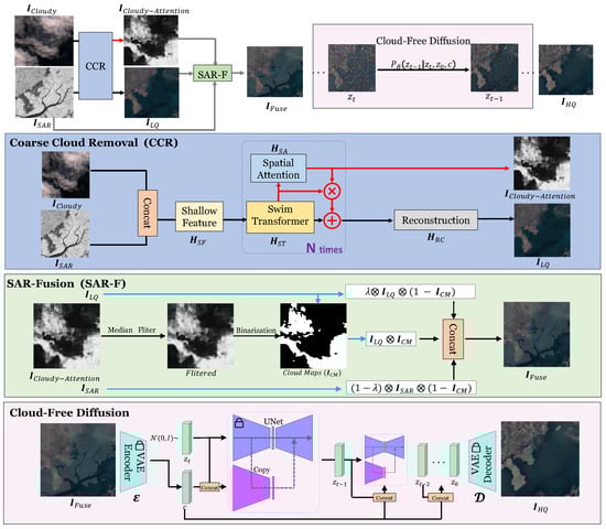
Figure 1.
Illustration of the flow of SAR-DeCR. Our proposed a three-stage model consists of to coarse cloud removal, SAR-Fusion, and cloud-free diffusion. In the coarse cloud removal state, SAR information is concatenated with thick cloud data, and cloud cover is mitigated through the feature extractor and the spatial attention module . In the subsequent stage, SAR-Fusion focuses on refining cloud attention to create a mask , which is then employed to selectively integrate SAR information, producing specifically in regions affected by cloud cover. In the final stage, the cloud-free diffusion (CF-D) module uses as an input, which acts as a visual condition. During training, is derived from a cloud-free image, and only the model weights of the duplicates are updated. In the inference phase, is randomly sampled from .
3.2. Coarse Cloud Removal
In the initial stage, as depicted in Figure 1, our methodology involves processing a cloud-obscured satellite remote sensing image, denoted as , alongside a SAR image, , which is rich in ground information. The primary goal in this stage is to perform a coarse cloud removal from . Given that lacks detailed ground information in areas covered by thick clouds, for this we concatenate with . Here, serves as a discriminative reference to supplement obscured ground information. This strategic combination enables the network to accomplish a preliminary texture reconstruction.
where Concat(·) denotes the concatenation of channels. The represents a 3 × 3 convolutional layer used to extract the initial shallow features, aiming to obtain . The deep feature extraction module is utilized to extract profound features from . Feature extraction is conducted to assimilate representative and distinctive textures from into ; simultaneously, provides essential color information. The module is primarily comprised of the Swin transformer and spatial attention components. First, the features are extracted through the Swin transformer, and then spatial guidance is performed through the use of spatial attention. The deep feature extraction module is expressed as follows:
where the Swin transformer block, denoted as , is conducted using Swin transformers [13]. represents the spatial attention block [13], and denotes the features at the corresponding i-th layer. The iteration, denoted N times in Figure 1, represents a Cloud attention module aimed at discerning and extracting the attention embedded within the deep features. This attention mechanism elucidates the spatial distribution of clouds, thereby guiding the network to effectively remove cloud coverage. The cloud attention module specifically highlights cloud dense areas within the network, aiming to direct enhanced focus towards these regions. It is expressed as follows:
Finally, a convolutional layer as a reconstruction module to restore depth features to the image , represented as
where is a 3 × 3 convolutional layer, and is the feature of the N-th layer.
3.3. SAR-Fusion
In the second stage, in Figure 2, the regions in corresponding to cloud-covered areas in display boxed shadows and noticeable blurring. These regions also show a significant lack of structural coherence.
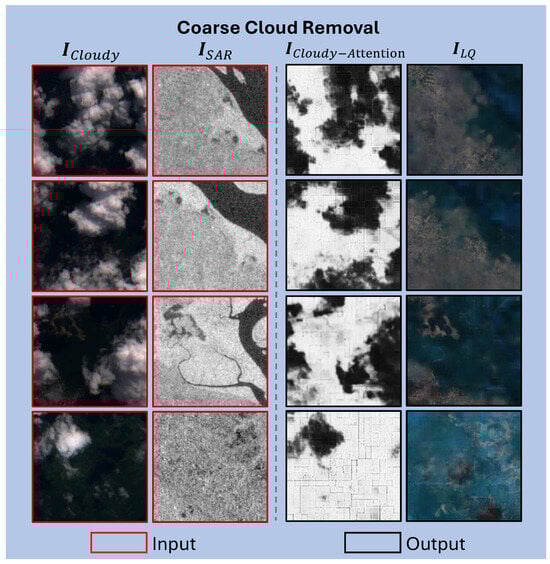
Figure 2.
Inputs and outputs of our coarse cloud removal (CCR) module. The inputs consist of (first column) and (second column), while the outputs are (third column) and (fourth column). Each row represents a different visualization example. When compared to , successfully recovers most information obstructed by clouds, including ground texture and color.
Specifically, these are the areas in that are covered by clouds, whereas areas not covered by clouds are restored. Our goal is to integrate ground structure information specifically in the regions affected by clouds, using data from . It is important to note that while effectively removes clouds, it often introduces blurry artifacts and noise. Additionally, it fails to reconstruct complex textures accurately. SAR-F includes filtering, binarization, and mixup operations. The primary function of SAR-F is to introduce more targeted ground information into areas where clouds have been removed by , guiding the learning process of the assisted diffusion model while ensuring minimal impact on other, cloud-free areas. The primary function of SAR-F is to provide targeted ground information to areas where clouds have been removed by . This guides the learning process of the assisted diffusion model while minimizing its impact on cloud-free regions.
The first step is to identify the locations of clouds as detected by the results of . Then, a median filter operation is applied to to reduce the impact of redundant artifacts, followed by binarization to produce the cloud map . The black area in (with a value of 0) indicates the presence of clouds, while the opposite represents cloud-free areas. We then use to segment . Firstly, the cloud area is preserved, as expressed by the formula: ). Next, we introduce SAR information into the cloud-occupied regions using a simple mixup operation with a mixing scale factor , which can be expressed as
where denotes the regions occupied by clouds, and 1 − represents the proportion of SAR information introduced.
3.4. Cloud-Free Diffusion
As shown in Figure 3, generated by SAR-Fusion in the previous state exhibits numerous blocky shadows and lacks intricate ground texture. To address this, we have introduced the cloud-free diffusion (CF-D) module, which utilizes the powerful texture generation capacities of diffusion models to further eliminate these shadows. In the third stage of our process, in Figure 4, we aim to restore a high-quality, clear image () from .
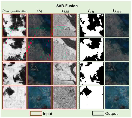
Figure 3.
Inputs and outputs of our SAR-Fusion (SAR-F) module. Initially, (first column) is filtered and binarized, resulting in the generation of (fourth column). Subsequently, (second column) and (third column) are combined under the guidance of to restore the missing complex texture in , thereby generating (fifth column).
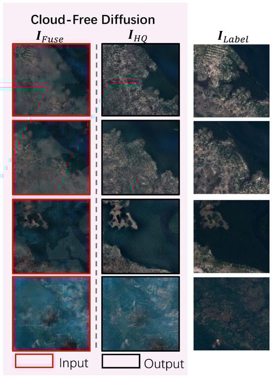
Figure 4.
Inputs and outputs of our cloud-free diffusion (CF-D) module. The diffusion model generates the (second column) and closely resembles the label (third column), exhibiting a notable enhancement in detail compared to (first column).
The CF-D module employs the robust generative capabilities of diffusion to reconstruct into a high-quality, cloud-free image. Specifically, we use a pre-trained variational autoencoder (VAE) [38] encoder to convert and into discrete vectors, c and , respectively, within the latent space. We replicate the encoder and middle layers of the U-Net to serve as trainable components. The input to this replica is a concatenation of c and , and the outputs are resized by a convolutional layer before being reintegrated into the U-Net decoder.
During training, a ground cloud-free image is transformed into the variable within the latent space via the VAE encoder. Then, noise is introduced to the variable. c represents the result () from the second stage (SAR-F) obtained through the encoder. Additionally, the weights of U-Net are frozen, while only the weights of the replica are updated. This strategy ensures that the robust generative capabilities acquired through stable diffusion are maintained. The replica plays a vital role in regulating the generation process. During inference, is randomly sampled from , following DDPM [9]. The is then reconstructed by mapping back to pixel space using a pre-trained VAE decoder.
3.5. Loss Function
Our model undergoes training in two stages, as outlined in Section 3.1, focusing on coarse cloud removal and high-quality image reconstruction in Algorithms 1 and 2.
Coarse Cloud Removal. The model is trained for coarse cloud removal to produce , which serves as a precursor to the subsequent stage of high-quality image reconstruction training. The loss associated with coarse cloud removal is bifurcated into two components. The first component involves pixel reconstruction, where the loss pertains to the output of the cloud removal process, , and the cloud-free image, . The subsequent component comprises the loss function related to cloudy attention, which aligns with the outputs of spatial attention and the binary map M. The map M is generated based on the difference between and , where represents a cloud-free image captured at the same location as within a time gap of fewer than 15 days [39]. The corresponding loss for coarse cloud removal is expressed as follows:
where and represent L1 regularization and L2 regularization, respectively.
Reconstruction via Latent Diffusion. The diffusion model is employed for the high-quality image reconstruction stage. This phase can be divided into two key processes: the forward diffusion phase and the backward sampling phase. In the forward diffusion phase, the initial data are corrupted by the addition of normal noise over a sequence of T iterations. The state of the data at time t can be represented as follows:
where indicates the weight term. The backward sampling process involves an iterative denoising procedure that transitions given noise to a clean state :
where , , and , with being the cumulative product from to .
represents a trainable noise estimate. The training loss of the diffusion model, encompassing both the real noise and the network predicted noise , is expressed as follows:
| Algorithm 1 SAR-DeCR Training. |
|
| Algorithm 2 DDPM sampling process. |
|
3.6. Discussion with Other Diffusion-Based DC Methods
Our approach introduces key innovations in data integration, generation mechanisms, and prior-guided enhancement. Unlike DiffCR [10] and DE [36], which depend solely on optical imagery, we incorporate SAR data to exploit their unique ability to penetrate dense clouds and retain ground information. A cloud-mask-based dynamic fusion strategy (SAR-F module) is developed. It effectively merges optical and SAR data, ensuring optimal performance in both cloudy and cloud-free regions. In the generation process, we use a cloud-free diffusion (CF-D) model in latent space. This model is guided by a pre-trained VEA, which transitions generation from pixel space to latent space for enhanced semantic coherence. To further refine detail generation in complex scenarios, we integrate ControlNet to streamline the process, reducing computational steps while maintaining precision. Additionally, we leverage preliminary results from the coarse cloud removal (CCR) stage as priors. These outputs are incorporated into the diffusion process, ensuring more robust structural and textural fidelity for heavily clouded areas. These advancements enable our method to deliver substantial improvements in texture, semantic richness, and detail fidelity for the generated images.
4. Experiment
4.1. Dataset
SEN12MS-CR Dataset. The dataset utilized, designated SEN12MS-CR, enhances the previously established SEN12MS dataset [40]. This research conducted in this study centers on satellite imagery sourced from the Sentinel satellites of the European Copernicus Earth observation program [41]. These data are selected due to their global availability and user-friendly access, making them highly suitable for our analytical purposes.
SEN12MS-CR [39] consists of 169 distinct regions of interest (ROIs) sampled from all inhabited continents and during meteorological seasons. Scene locations are randomly selected from two uniform distributions: one covering all landmasses and another focusing solely on urban areas. This introduces a bias toward urban landscapes, which are often the focus of remote sensing studies due to their more complex patterns. Each ROI measures approximately pixels, translating to km on the ground, with each pixel representing a 10-m ground sampling distance. Each ROI includes a triplet of orthorectified, georeferenced images: cloudy and cloud-free Sentinel-2 images, along with the corresponding Sentinel-1 image. To minimize the effects of surface changes, all images are captured within the same meteorological season. Cloud-free Sentinel-2 images are selected based on a maximum of 10% cloud coverage, while the selection for cloudy images ranges from 20% to 70% cloud coverage. The Sentinel-2 data are derived from the Level-1C top-of-atmosphere reflectance product, encompassing a range from 0 to 10,000 and including all 13 original bands. The Sentinel-1 data originate from the Level-1 GRD product, acquired in IW mode with two polarization channels (VV and VH).
Synthetic Dataset. The most effective strategy for classifying cloudy images involves assessing the percentage of cloud coverage. When cloud cover exceeds 60%, the optical image is predominantly obscured, rendering the underlying scene largely inaccessible [42]. To address this challenge, the SEN12MS-CR cloud-free image dataset has been augmented with clouds at 30%, 60%, and 90% coverage, with the 90% addition specifically designed to simulate more complex cloud conditions. To demonstrate that our module surpasses other SOTA methods in cloud removal, we conducted an experiment using a cloud-augmented dataset. The process of adding clouds was carried out using the satellite cloud generator [43] (satellite cloud generator https://github.com/strath-ai/SatelliteCloudGenerator, accessed on 23 August 2023), which facilitates the creation of synthetic cloud environments. A single experiment focused on removing clouds from the SEN12MS-CR dataset.
4.2. Implementation Details
Parameter Settings. The model’s training phase is structured in two stages, each tailored to address specific elements of the loss function.
The first training stage, focused on coarse cloud removal, employs the Adam optimizer [44]. This stage involves training over 200 epochs, beginning with a learning rate of and a batch size of 4. The feature extraction layer utilizes a Swin transformer [12], comprising three layers with a window size of 16 and dimensions for the intermediate and embedding layers set at 96. The feature extraction layer consists of 3 layers with a window size of 16.
For the second training stage, which focuses on image reconstruction, we employ both UNet and Replica networks, adhering to the setup specified by DiffBIR [45]. For the VAE, we utilize an encoder and decoder architecture based on the VQ-VAE [38]. This stage of training encompasses 100 epochs, starting with a learning rate of and a batch size of 8. During inference, we set the number of samples for the DDPM to 50. The weighting factor is initially set at 1.0.
Benchmarks and Metrics. To assess the effectiveness of our approach, we conduct both training and testing using the extensive SEN12MS-CR dataset [39], which consists of triplets of cloudy images, cloud-free images, and their SAR counterparts, each with dimensions of pixels.
To evaluate the efficacy of SOTA methods, we utilize two reference metrics, peak signal-to-noise ratio (PSNR) and structural similarity index (SSIM), and two no-reference metrics, natural image quality evaluator (NIQE) [46] and multidimension attention network for no-reference image quality assessment (MANIQA) [47]. The reference metrics assess the accuracy of pixel recovery in the reconstructed image, whereas the no-reference metrics gauge the realism and overall quality of the image. To ensure the impartiality and accuracy of our assessment, we employ Tool IQA [48,49] (IQA Tool https://github.com/chaofengc/IQA-PyTorch, accessed on 31 August 2022) to compute these four key indicators.
4.3. Comparison with the State of the Art
We conduct a comparison of our method with other SOTA cloud removal methods to provide a thorough analysis. These methods include Spa-GAN [50], which does not utilize SAR guidance, and more recently introduced SAR-guided methods such as DSen2-CR [3], GLF-CR [7], and UnCRtainTS L2 [8]. The evaluation encompasses both quantitative and qualitative analyses.
Quantitative analysis: SEN12MS-CR Dataset. Table 1 presents the quantitative metrics for our method alongside other SOTA methods, incorporating both reference and no-reference metrics. The data in Table 1 underscore the superior performance of our method, which notably achieves a PSNR above 20 and an SSIM above 0.55, figures that are significantly higher than those recorded for competing methods. Additionally, when compared to other methods like Spa-GAN (0.22M), DSen2-CR (18.95M), GLF-CR (14.83M), and UnCRtainTS L2 (0.57M). Our approach uses a much larger model, with a total of 852.03 million parameters. This total is made up of two components: the parameters from the CCR in the first stage and the U-Net (copy) portion in the CF-D of the third stage. Moreover, at the juncture where reference metrics are optimized, no-reference metrics similarly peak. Notably, MANIQA is the only metric exceeding 0.5 across all methods, affirming the robustness of our approach.

Table 1.
The quantitative comparison of our proposed method with other cloud removal methods. Our method (SAR-DeCR) exhibits superior performance compared to all other methods on the SEN12MS-CR dataset.
Synthetic Dataset. The quantitative results, shown in Table 2, indicate that as cloud coverage increases (from 30% to 60% and 90%), our method consistently outperforms others, such as SPA-GAN and UnCRtainTS L2, in terms of PSNR and SSIM. Remarkably, at 90% cloud coverage, our method achieves PSNR and SSIM values of 20.9157 and 0.5530, respectively, demonstrating its robustness in restoring the original image even under heavy cloud conditions. Additionally, our method excels in no-reference quality metrics (NIQE and MANIQA), with lower NIQE and higher MANIQA scores, indicating superior visual quality and fidelity.
Table 2.
In the SEN12MS-CR dataset, our proposed method demonstrates superior performance compared to other cloud removal methods. Additionally, a percentage addition cloud experiment is conducted on the cloud-free data in the dataset. The addition of clouds at 30%, 60%, and 90%, respectively, yields results that closely resemble those of the original dataset.
Qualitative analysis: SEN12MS-CR Dataset. Figure 5 provides a visual comparison of the cloud removal capabilities of the discussed methods. Spa-GAN demonstrates limited effectiveness in removing thick clouds, thereby highlighting the value of SAR guidance. Conversely, while SAR-guided methods manage coarse cloud removal, they significantly lack in detail reconstruction within the cloudy regions. In stark contrast, our method not only effectively removes clouds but also excels in reconstructing detailed textures within these regions.
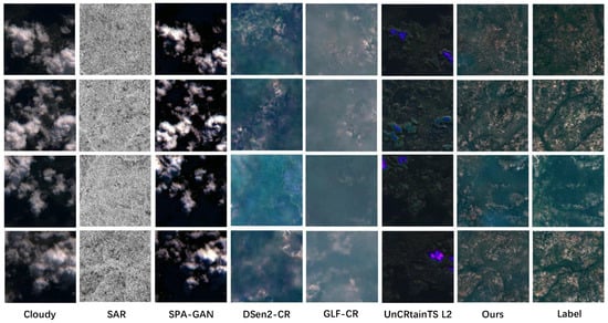
Figure 5.
The qualitative analysis of the proposed and existing methods: Spa-GAN [50], DSen2-CR [3], GLF-CR [7], and UnCRtainTS L2 [8], for thick cloud removal performance in different natural environments on the SEN12MS-CR dataset [39].
Synthetic Dataset. Figure 6 illustrates that our method can accurately restore ground truth textures and details in images with varying cloud coverages. In contrast, SPA-GAN tends to blur and distort under high cloud cover, and UnCRtainTS L2 struggles with detail processing. Our algorithm consistently produces generating results that closely resemble the original cloud-free images under various cloud coverage scenarios. Notably, under 90% cloud coverage, the images are essentially consistent with the cloud-free label images, showcasing exceptional capabilities in overcoming cloud occlusion.
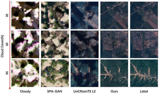
Figure 6.
This figure visually compares the cloud removal performance of three methods: SPA-GAN, UnCRtainTS L2, and our proposed method across different levels of cloud coverage (30%, 60%, and 90%). The first column shows the synthetic cloudy images at each coverage level, while the second and third columns show the results from SPA-GAN and UnCRtainTS L2, respectively. The fourth column presents the results from our method, which closely resemble the ground truth images shown in the fifth column. As cloud coverage increases, our method consistently produces clearer and more accurate images, effectively restoring details even with 90% cloud coverage.
4.4. Ablation Study
We conduct ablation experiments on our proposed modules using the processed SEN12MS-CR dataset.
As depicted in Table 3, (1) “#1” tests the CCR process without the implementation of the SAR-F and CF-D modules we proposed. This experiment aims to verify the individual effectiveness of the CF-D and SAR-F modules. (2) “#2” evaluates the impact of our proposed SAR-F module in isolation. Unlike the full implementation of our method, “#2” omits SAR-F while maintaining the rest of the experimental setup identical to the full configuration. (3) “#3” underscores the significance of CF-D to our model. The enhancements in detail and texture observed in our results would not have been achievable without the integration of CF-D.
Table 3.
Ablation study of SAR-F and CF-D. Each proposed component is analyzed independently. The row in bold in the table has the best indicator.
The quantitative results in Table 3 for “#1” and “#2” show a marked improvement in performance metrics for “#2”, underscoring the substantial impact of the CF-D module on image reconstruction quality. Furthermore, the comparisons between “#3” and “ours full” demonstrate that the robust generative capabilities of the diffusion model are a key component of our methodology, significantly enhancing the overall efficacy of the model. The CF-D module leverages the diffusion model’s capabilities to reconstruct complex details in cloudy regions effectively. Additionally, the metric improvements observed in “#2” and “ours full” indicate that integrating specific SAR ground information through the SAR-F module enables the diffusion model to generate more refined details leading to the synthesis of more realistic and precise texture details. The data for “#1” and “#3” further confirm that SAR-F’s guidance significantly enhances the model’s ability to render detailed and appropriate textures. The indispensable roles of both SAR-F and CF-D modules are evident when comparing the results across “our full”, “#2”, and “#3”.
Cloud Attention. To illustrate the enhanced performance of our approach, we undertake a comparative of the binary images generated by s2cloudless [51] with . In s2cloudless, cloud masking requires Sentinel-2 data (from digital numbers to reflectances), posing a significant limitation as only a few products meet these conditions and many sensors are not designed to capture such spectral details. So our method has more advantages in channels. Additionally, the availability and range of spectral bands may vary between sensors. For example, lower-resolution imaging platforms like Landsat-8 and Sentinel-2 typically provide broader, though distinct, spectrum coverage. In contrast, higher-resolution imagery from platforms such as SkySat may only include visible RGB channels and near-infrared [52]. We have pre-processed the test dataset according to the product baseline 04.00. Additional harmonization adjustments were applied to the data following ESA guidelines (https://sentinels.copernicus.eu/en/web/sentinel/-/copernicus-sentinel-2-major-products-upgrade-upcoming, accessed on 29 September 2021). In the second stage of SAR-Fusion, the input image, designated as , is converted into a binary image using the s2cloudless algorithm. Subsequent experiments follow this same methodology.
As shown in Table 4, our model demonstrates modest improvements across all metrics, including PSNR, SSIM, NIQE, and MANIQA. This indicates that the images generated by our model more accurately represent cloudy regions. The final visualization, presented in Figure 7, shows that the overall differences are not substantial. However, discrepancies in texture preservation suggest that our method is more effective at retaining detail. The binary results reveal that the cloud mask generated by the s2cloudless method lacks detail compared to the mask produced by our method. Furthermore, the output from the s2cloudless method results in coarser cloud occlusion area with unclear boundaries, which diminishes its ability to accurately depict the complex morphology of cloud formations. In contrast, our method generates a more detailed cloud structure in the binary results. This allows for more accurate separation of cloud blocks from non-cloud areas, producing a refined cloud mask with smoother edges.
Table 4.
Quantitative comparison of our proposed cloud attention and s2cloudless. All four values show a small improvement.

Figure 7.
Cloudy is the original cloud map. The third column represents the binary image obtained by applying the s2cloudless method [51] to the cloud map. The following visualization demonstrates the discrepancy between the outcomes yielded by the cloud mask (s2cloudless) and our cloud attention approach. All experimental parameters remain constant, with the exception of the replacement of with the output of s2cloudless. As shown in the figure, the results obtained by the two methods are roughly similar. Comparing the second and third columns, we can see that the cloud attention method provides a more complete representation of some details. The fourth column shows the results generated by s2cloudless, and the fifth column shows the images generated by our method (SAR-DeCR). The last column shows the integrated cloud-free ground image.
SAR Coefficient. The analyses presented in Table 5 and Figure 8, demonstrate that varying the values of significantly impacts the effectiveness of image fusion.
Table 5.
In the SAR-Fusion module, we set to 1 to exclude . The results are presented in the following table, which demonstrates that all four indicators achieve optimal performance when is set to 0.9. The best indicators in the table are in bold.
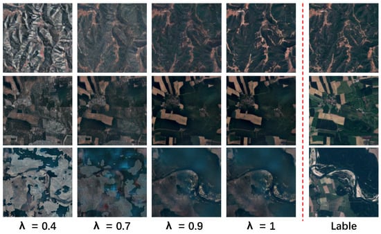
Figure 8.
This figure illustrates the impact of varying the parameter on the visualization results of images when employing SAR data for cloud removal. The first three columns display results with different values (0.4, 0.7, and 0.9), demonstrating progressive improvements in detail and texture as increases. The fourth column shows the results without SAR data ( = 1), which lack the same level of detail. The final column displays the cloud-free ground truth image. When is set to 0.9, the generated image closely matches the ground truth in terms of texture and detail, underscoring the benefits of integrating SAR data with an optimal setting.
From a visual perspective, as shown in Figure 8, adjusting the value of allows for the manipulation of details and textures within the image. At = 0.4, the image contains more numerous fused SAR components, resulting in greater roughness in its details and textures. Conversely, at = 0.9, the image more closely approximates the details and texture of the real cloud-free image, displaying enhanced clarity and authenticity. In conclusion, the value of is crucial in determining both the quality and visual attributes of the fused image. This study identifies = 0.9 as the optimal parameter setting for the SAR fusion module, yielding the most favorable quantitative and qualitative results.
Quantitative evaluations shown in Figure 9 reveal that as the value of increases, both the PSNR and the SSIM of the image exhibit a gradual upward trend. At a value of 0.9, these indicators reach their peak values, 21.3601 and 0.5784, respectively. Additionally, as depicted in Table 5, the non-reference quality evaluation metrics NIQE and MANIQA show improved performance at = 0.9, indicating an increase in resemblance to the actual cloud-free image.
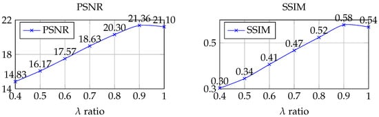
Figure 9.
During the process of selecting in accordance with Equation (5), numerous tests were conducted. Considering that the FR method depends on reference images and is applicable to scenarios with available reference data, we ultimately selected PSNR and SSIM as the preferred evaluation metrics. The overall results indicate that the impact of is inversely proportional to the size of . As increases, the image quality indicators PSNR and SSIM also show improvement.
5. Conclusions
We introduce a method for removing thick clouds from satellite remote-sensing imagery, termed SAR-DeCR. This approach is designed to restore high-quality images that are recognizably guided by SAR ground information, ensuring accurate geographic information retrieval. Our method begins with the integration of the thick cloud image and the SAR image to effectively eliminate cloud obstructions, which typically obscure ground information, called coarse cloud removal (CCR). In CCR, the Swin transformer serves as the feature extractor, and the spatial attention model provides the Swin transformer with the approximate location information of the cloud. Subsequently, we introduce the SAR-Fusion (SAR-F) module to refine the initial output of the coarse cloud removal and to enhance the influence of SAR data. SAR-F effectively incorporates SAR data into cloud positions in an unsupervised manner, thereby augmenting the guidance provided by SAR information. Lastly, to capitalize on the powerful generative capabilities of expansive vision-text models, and to use the fused images as conditional supervision, we develop a high-fidelity information reconstruction module based on the diffusion model, called cloud-free diffusion (CF-D). CF-D is specifically designed to preserve accurate SAR ground information and to complement the remaining high-frequency information. Our experiments clearly demonstrate the superiority of our approach over other SOTA SAR-guided methods. Notably, our proposed model is the first application of diffusion modeling in the realm of SAR-guided thick cloud removal, providing valuable insights for future research.
Author Contributions
All authors designed the methodology. Y.S. (Yexing Song) implemented the methodology and performed the statistical analysis; all authors contributed to the analysis of the data, interpretation of the results, and the writing of the paper. All authors have read and agreed to the published version of the manuscript.
Funding
This research received no external funding.
Data Availability Statement
The source code of SAR-DeCR can be found at https://github.com/hshhhhhh123/SAR-DeCR, accessed on 25 June 2025.
Conflicts of Interest
The authors declare no conflicts of interest.
References
- Bermudez, J.; Happ, P.; Oliveira, D.; Feitosa, R. SAR to optical image synthesis for cloud removal with generative adversarial networks. ISPRS Ann. Photogramm. Remote Sens. Spat. Inf. Sci. 2018, 4, 5–11. [Google Scholar] [CrossRef]
- Goodfellow, I.; Pouget-Abadie, J.; Mirza, M.; Xu, B.; Warde-Farley, D.; Ozair, S.; Courville, A.; Bengio, Y. Generative adversarial networks. Commun. ACM 2020, 63, 139–144. [Google Scholar] [CrossRef]
- Meraner, A.; Ebel, P.; Zhu, X.X.; Schmitt, M. Cloud removal in Sentinel-2 imagery using a deep residual neural network and SAR-optical data fusion. ISPRS J. Photogramm. Remote Sens. 2020, 166, 333–346. [Google Scholar] [CrossRef] [PubMed]
- He, K.; Zhang, X.; Ren, S.; Sun, J. Deep residual learning for image recognition. In Proceedings of the IEEE Conference on Computer Vision and Pattern Recognition 2016, Las Vegas, NV, USA, 27–30 June 2016; pp. 770–778. [Google Scholar]
- Han, S.; Wang, J.; Zhang, S. Former-CR: A Transformer-Based Thick Cloud Removal Method with Optical and SAR Imagery. Remote Sens. 2023, 15, 1196. [Google Scholar] [CrossRef]
- Vaswani, A.; Shazeer, N.; Parmar, N.; Uszkoreit, J.; Jones, L.; Gomez, A.N.; Kaiser, Ł.; Polosukhin, I. Attention is all you need. Adv. Neural Inf. Process. Syst. 2017, 30, 6000–6010. [Google Scholar]
- Xu, F.; Shi, Y.; Ebel, P.; Yu, L.; Xia, G.S.; Yang, W.; Zhu, X.X. GLF-CR: SAR-enhanced cloud removal with global–local fusion. ISPRS J. Photogramm. Remote Sens. 2022, 192, 268–278. [Google Scholar] [CrossRef]
- Ebel, P.; Garnot, V.S.F.; Schmitt, M.; Wegner, J.D.; Zhu, X.X. UnCRtainTS: Uncertainty Quantification for Cloud Removal in Optical Satellite Time Series. In Proceedings of the IEEE/CVF Conference on Computer Vision and Pattern Recognition 2023, Vancouver, BC, Canada, 17–24 June 2023; pp. 2085–2095. [Google Scholar]
- Ho, J.; Jain, A.; Abbeel, P. Denoising diffusion probabilistic models. Adv. Neural Inf. Process. Syst. 2020, 33, 6840–6851. [Google Scholar]
- Zou, X.; Li, K.; Xing, J.; Zhang, Y.; Wang, S.; Jin, L.; Tao, P. DiffCR: A Fast Conditional Diffusion Framework for Cloud Removal From Optical Satellite Images. IEEE Trans. Geosci. Remote Sens. 2024, 62, 5612014. [Google Scholar] [CrossRef]
- Xiao, Y.; Yuan, Q.; Jiang, K.; He, J.; Jin, X.; Zhang, L. EDiffSR: An Efficient Diffusion Probabilistic Model for Remote Sensing Image Super-Resolution. IEEE Trans. Geosci. Remote Sens. 2024, 62, 5601514. [Google Scholar] [CrossRef]
- Liu, Z.; Lin, Y.; Cao, Y.; Hu, H.; Wei, Y.; Zhang, Z.; Lin, S.; Guo, B. Swin transformer: Hierarchical vision transformer using shifted windows. In Proceedings of the IEEE/CVF International Conference on Computer Vision 2021, Montreal, QC, Canada, 10–17 October 2021; pp. 10012–10022. [Google Scholar]
- Wang, T.; Yang, X.; Xu, K.; Chen, S.; Zhang, Q.; Lau, R.W. Spatial attentive single-image deraining with a high quality real rain dataset. In Proceedings of the IEEE/CVF Conference on Computer Vision and Pattern Recognition 2019, Long Beach, CA, USA, 15–20 June 2019; pp. 12270–12279. [Google Scholar]
- Zhang, L.; Rao, A.; Agrawala, M. Adding conditional control to text-to-image diffusion models. In Proceedings of the IEEE/CVF International Conference on Computer Vision 2023, Paris, France, 1–6 October 2023; pp. 3836–3847. [Google Scholar]
- Zhang, Y.; Guindon, B.; Cihlar, J. An image transform to characterize and compensate for spatial variations in thin cloud contamination of Landsat images. Remote Sens. Environ. 2002, 82, 173–187. [Google Scholar] [CrossRef]
- Shen, H.; Li, H.; Qian, Y.; Zhang, L.; Yuan, Q. An effective thin cloud removal procedure for visible remote sensing images. ISPRS J. Photogramm. Remote Sens. 2014, 96, 224–235. [Google Scholar] [CrossRef]
- Li, J.; Hu, Q.; Ai, M. Haze and thin cloud removal via sphere model improved dark channel prior. IEEE Geosci. Remote Sens. Lett. 2018, 16, 472–476. [Google Scholar] [CrossRef]
- He, K.; Sun, J.; Tang, X. Single image haze removal using dark channel prior. IEEE Trans. Pattern Anal. Mach. Intell. 2010, 33, 2341–2353. [Google Scholar] [PubMed]
- Shen, H.; Zhang, C.; Li, H.; Yuan, Q.; Zhang, L. A spatial–spectral adaptive haze removal method for visible remote sensing images. IEEE Trans. Geosci. Remote Sens. 2020, 58, 6168–6180. [Google Scholar] [CrossRef]
- Han, Y.; Yin, M.; Duan, P.; Ghamisi, P. Edge-preserving filtering-based dehazing for remote sensing images. IEEE Geosci. Remote Sens. Lett. 2021, 19, 8019105. [Google Scholar] [CrossRef]
- Xu, M.; Jia, X.; Pickering, M.; Jia, S. Thin cloud removal from optical remote sensing images using the noise-adjusted principal components transform. ISPRS J. Photogramm. Remote Sens. 2019, 149, 215–225. [Google Scholar] [CrossRef]
- Li, B.; Gou, Y.; Gu, S.; Liu, J.Z.; Zhou, J.T.; Peng, X. You only look yourself: Unsupervised and untrained single image dehazing neural network. Int. J. Comput. Vis. 2021, 129, 1754–1767. [Google Scholar] [CrossRef]
- Gandelsman, Y.; Shocher, A.; Irani, M. “Double-DIP”: Unsupervised image decomposition via coupled deep-image-priors. In Proceedings of the IEEE/CVF Conference on Computer Vision and Pattern Recognition, Long Beach, CA, USA, 15–20 June 2019; pp. 11026–11035. [Google Scholar]
- Li, B.; Gou, Y.; Liu, J.Z.; Zhu, H.; Zhou, J.T.; Peng, X. Zero-shot image dehazing. IEEE Trans. Image Process. 2020, 29, 8457–8466. [Google Scholar] [CrossRef]
- Yu, X.; Pan, J.; Wang, M.; Xu, J. A curvature-driven cloud removal method for remote sensing images. Geo-Spat. Inf. Sci. 2024, 27, 1326–1347. [Google Scholar] [CrossRef]
- Chen, Y.; Chen, M.; He, W.; Zeng, J.; Huang, M.; Zheng, Y.B. Thick cloud removal in multitemporal remote sensing images via low-rank regularized self-supervised network. IEEE Trans. Geosci. Remote Sens. 2024, 62, 5506613. [Google Scholar] [CrossRef]
- Jin, M.; Wang, P.; Li, Y. HyA-GAN: Remote sensing image cloud removal based on hybrid attention generation adversarial network. Int. J. Remote Sens. 2024, 45, 1755–1773. [Google Scholar] [CrossRef]
- Jia, J.; Pan, M.; Li, Y.; Yin, Y.; Chen, S.; Qu, H.; Chen, X.; Jiang, B. GLTF-Net: Deep-learning network for thick cloud removal of remote sensing images via global–local temporality and features. Remote Sens. 2023, 15, 5145. [Google Scholar] [CrossRef]
- Zhang, Y.; Ji, L.; Xu, X.; Zhang, P.; Jiang, K.; Tang, H. A flexible spatiotemporal thick cloud removal method with low requirements for reference images. Remote Sens. 2023, 15, 4306. [Google Scholar] [CrossRef]
- Xiang, X.; Tan, Y.; Yan, L. Cloud-Guided Fusion with SAR-to-Optical Translation for Thick Cloud Removal. IEEE Trans. Geosci. Remote Sens. 2024, 62, 5633715. [Google Scholar] [CrossRef]
- Liu, G.; Qiu, J.; Yuan, Y. A Multi-Level SAR-Guided Contextual Attention Network for Satellite Images Cloud Removal. Remote Sens. 2024, 16, 4767. [Google Scholar] [CrossRef]
- Rombach, R.; Blattmann, A.; Lorenz, D.; Esser, P.; Ommer, B. High-resolution image synthesis with latent diffusion models. In Proceedings of the IEEE/CVF Conference on Computer Vision and Pattern Recognition 2022, New Orleans, LA, USA, 18–24 June 2022; pp. 10684–10695. [Google Scholar]
- Esser, P.; Rombach, R.; Ommer, B. Taming transformers for high-resolution image synthesis. In Proceedings of the IEEE/CVF Conference on Computer Vision and Pattern Recognition 2021, Nashville, TN, USA, 20–25 June 2021; pp. 12873–12883. [Google Scholar]
- Song, J.; Meng, C.; Ermon, S. Denoising diffusion implicit models. arXiv 2020, arXiv:2010.02502. [Google Scholar]
- Zhao, X.; Jia, K. Cloud removal in remote sensing using sequential-based diffusion models. Remote Sens. 2023, 15, 2861. [Google Scholar] [CrossRef]
- Sui, J.; Ma, Y.; Yang, W.; Zhang, X.; Pun, M.O.; Liu, J. Diffusion Enhancement for Cloud Removal in Ultra-Resolution Remote Sensing Imagery. IEEE Trans. Geosci. Remote Sens. 2024, 62, 5405914. [Google Scholar] [CrossRef]
- Jing, R.; Duan, F.; Lu, F.; Zhang, M.; Zhao, W. Denoising diffusion probabilistic feature-based network for cloud removal in Sentinel-2 imagery. Remote Sens. 2023, 15, 2217. [Google Scholar] [CrossRef]
- Van Den Oord, A.; Vinyals, O. Neural discrete representation learning. Adv. Neural Inf. Process. Syst. 2017, 30, 6309–6318. [Google Scholar]
- Ebel, P.; Meraner, A.; Schmitt, M.; Zhu, X.X. Multisensor data fusion for cloud removal in global and all-season sentinel-2 imagery. IEEE Trans. Geosci. Remote Sens. 2020, 59, 5866–5878. [Google Scholar] [CrossRef]
- Schmitt, M.; Hughes, L.H.; Qiu, C.; Zhu, X.X. SEN12MS–A curated dataset of georeferenced multi-spectral sentinel-1/2 imagery for deep learning and data fusion. arXiv 2019, arXiv:1906.07789. [Google Scholar] [CrossRef]
- Desnos, Y.L.; Borgeaud, M.; Doherty, M.; Rast, M.; Liebig, V. The European Space Agency’s earth observation program. IEEE Geosci. Remote Sens. Mag. 2014, 2, 37–46. [Google Scholar] [CrossRef]
- Maalouf, A.; Carré, P.; Augereau, B.; Fernandez-Maloigne, C. A bandelet-based inpainting technique for clouds removal from remotely sensed images. IEEE Trans. Geosci. Remote Sens. 2009, 47, 2363–2371. [Google Scholar] [CrossRef]
- Czerkawski, M.; Atkinson, R.; Michie, C.; Tachtatzis, C. SatelliteCloudGenerator: Controllable Cloud and Shadow Synthesis for Multi-Spectral Optical Satellite Images. Remote Sens. 2023, 15, 4138. [Google Scholar] [CrossRef]
- Kingma, D.P.; Ba, J. Adam: A method for stochastic optimization. arXiv 2014, arXiv:1412.6980. [Google Scholar]
- Lin, X.; He, J.; Chen, Z.; Lyu, Z.; Fei, B.; Dai, B.; Ouyang, W.; Qiao, Y.; Dong, C. DiffBIR: Towards Blind Image Restoration with Generative Diffusion Prior. arXiv 2023, arXiv:2308.15070. [Google Scholar]
- Mittal, A.; Soundararajan, R.; Bovik, A.C. Making a “completely blind” image quality analyzer. IEEE Signal Process. Lett. 2012, 20, 209–212. [Google Scholar] [CrossRef]
- Yang, S.; Wu, T.; Shi, S.; Lao, S.; Gong, Y.; Cao, M.; Wang, J.; Yang, Y. Maniqa: Multi-dimension attention network for no-reference image quality assessment. In Proceedings of the IEEE/CVF Conference on Computer Vision and Pattern Recognition, New Orleans, LA, USA, 18–24 June 2022; pp. 1191–1200. [Google Scholar]
- Chen, C.; Mo, J.; Hou, J.; Wu, H.; Liao, L.; Sun, W.; Yan, Q.; Lin, W. TOPIQ: A Top-Down Approach From Semantics to Distortions for Image Quality Assessment. IEEE Trans. Image Process. 2024, 33, 2404–2418. [Google Scholar] [CrossRef]
- Wu, H.; Zhang, Z.; Zhang, W.; Chen, C.; Li, C.; Liao, L.; Wang, A.; Zhang, E.; Sun, W.; Yan, Q.; et al. Q-Align: Teaching LMMs for Visual Scoring via Discrete Text-Defined Levels. In Proceedings of the International Conference on Machine Learning (ICML) 2024, Vienna, Austria, 21–27 July 2024. [Google Scholar]
- Pan, H. Cloud removal for remote sensing imagery via spatial attention generative adversarial network. arXiv 2020, arXiv:2009.13015. [Google Scholar]
- Skakun, S.; Wevers, J.; Brockmann, C.; Doxani, G.; Aleksandrov, M.; Batič, M.; Frantz, D.; Gascon, F.; Gómez-Chova, L.; Hagolle, O.; et al. Cloud Mask Intercomparison eXercise (CMIX): An evaluation of cloud masking algorithms for Landsat 8 and Sentinel-2. Remote Sens. Environ. 2022, 274, 112990. [Google Scholar] [CrossRef]
- Xie, Y.; Li, Z.; Bao, H.; Jia, X.; Xu, D.; Zhou, X.; Skakun, S. Auto-CM: Unsupervised deep learning for satellite imagery composition and cloud masking using spatio-temporal dynamics. In Proceedings of the AAAI Conference on Artificial Intelligence 2023, Washington DC, USA, 7–14 February 2023; Volume 37, pp. 14575–14583. [Google Scholar]
Disclaimer/Publisher’s Note: The statements, opinions and data contained in all publications are solely those of the individual author(s) and contributor(s) and not of MDPI and/or the editor(s). MDPI and/or the editor(s) disclaim responsibility for any injury to people or property resulting from any ideas, methods, instructions or products referred to in the content. |
© 2025 by the authors. Licensee MDPI, Basel, Switzerland. This article is an open access article distributed under the terms and conditions of the Creative Commons Attribution (CC BY) license (https://creativecommons.org/licenses/by/4.0/).