Article

Burned Area Detection in the Eastern Canadian Boreal Forest Using a Multi-Layer Perceptron and MODIS-Derived Features

1
Institute of Environment Sciences, Department of Biology Sciences, University of Quebec at Montreal, Montreal, QC H2X 3Y7, Canada
2
Ontario Forest Research Institute, Ministry of Natural Resources, 1235 Queen Street East, Sault Ste. Marie, ON P6A 2E5, Canada
3
Department of Computer Science, University of Quebec at Montreal, Montreal, QC H2X 3Y7, Canada
*
Author to whom correspondence should be addressed.
Remote Sens. 2025, 17(13), 2162; https://doi.org/10.3390/rs17132162
Submission received: 4 May 2025 / Revised: 14 June 2025 / Accepted: 21 June 2025 / Published: 24 June 2025

Abstract

Wildfires play a critical role in boreal forest ecosystems, yet their increasing frequency poses significant challenges for carbon emissions, ecosystem stability, and fire management. Accurate burned area detection is essential for assessing post-fire landscape recovery and fire-induced carbon fluxes. This study develops, compares, and optimizes machine learning (ML)-based models for burned area classification in the eastern Canadian boreal forest from 2000 to 2023 using MODIS-derived features extracted from Google Earth Engine (GEE), and the feature extraction includes maximum, minimum, mean, and median values per feature to enhance spectral representation and reduce noise. The dataset was randomly split into training (70%), validation (15%), and testing (15%) sets for model development and assessment. Combined labels were used due to class imbalance, and the model performance was assessed using kappa and the F1-score. Among the ML techniques tested, deep learning (DL) with a Multi-Layer Perceptron (MLP) outperformed Support Vector Machines (SVMs) and Random Forest (RF) by demonstrating superior classification accuracy in detecting burned area. It achieved an F1-score of 0.89 for burned pixels, confirming its potential for improving the long-term wildfire monitoring and management in boreal forests. Despite the computational demands of processing large-scale remote sensing data at 250 m resolution, the MLP modeling approach that we used provides an efficient, effective, and scalable solution for long-term burned area detection. These findings underscore the importance of tuning both network architecture and regularization parameters to improve the classification of burned pixels, enhancing the model robustness and generalizability.

1. Introduction

Wildfires are among the most destructive natural disturbances, profoundly affecting terrestrial ecosystems, air quality, biodiversity, and human safety. In recent decades, the frequency, intensity, and scale of wildfires have increased globally, primarily due to multiple global change drivers, such as climate change [1], land use changes, and direct human action [2]. While globally, wildfire trends do not always show a uniform increase in burned area, many regions have experienced more frequent and intense fires, leading to larger and more severe wildfires [3]. Recent assessments suggest that changes in fire regimes have accelerated nearly ten-fold over the past 250 years, compared to rates during the rest of the Holocene. Boreal forests, tropical ecosystems, and fire-prone temperate regions are particularly vulnerable to future intensification—especially under high-emission scenarios [4]. This is particularly evident in Canada, which is home to over 28% of the global boreal forest [5] and has witnessed a marked rise in high-severity fire events, especially in its fire-prone forested landscapes [6]. In combination with warmer temperatures, prolonged fire seasons, reduced precipitation, and increased lightning activity [7], accidental or deliberate human-induced fire ignition [8] are further exacerbating the wildfire risks and have contributed to larger burned areas and intensified fire behavior [9]. However, fire regimes across Canada vary spatially due to the differences in land cover, ignition sources, and fire suppression strategies, highlighting the interplay between natural climatic factors and human-driven influences, necessitating region-specific wildfire management strategies [10]. The role of fire in boreal forest ecosystems is well-documented, including influencing carbon dynamics, altering net primary productivity (NPP), and affecting long-term ecosystem stability [11,12]. Recent studies emphasize that frequent and high-intensity wildfires are disrupting the boreal carbon balance, as fire disturbances accelerate forest carbon release, alter biomass recovery patterns, and shift the long-term carbon storage dynamics [13,14]. The increasing prevalence of such wildfires was exemplified by the 2023 wildfire season in Canada, which was unprecedented, with approximately 15 million hectares burned—nearly seven times the historical average recorded from 1986 to 2022 [15]. This escalation in fire activity reflects a broader trend in which Canadian forests have become more prone to high-severity fires over the past few decades, driven by changes in vegetation structure, fuel availability, and climate-induced drying patterns, all of which have contributed to greater fire intensity and larger burned areas in recent years [16]. These alarming trends underscore the urgent need for advanced and accurate burned area detection techniques to enhance fire management, ecological recovery planning, and long-term wildfire mitigation strategies.
Remote sensing is a crucial tool in wildfire detection, providing high-resolution, real-time data that enhance the monitoring and management efforts [17]. Wildfires are among the most significant disturbances affecting forest ecosystems, while other environmental stressors, such as droughts and insect infestations, indirectly contribute to the fire risk by altering the fuel availability. Traditional methods often fail to capture these subtle changes, but advancements in remote sensing techniques, including time series-based algorithms such as Composite2Change and Landsat imagery, have significantly improved disturbance detection and wildfire monitoring [18]. Satellite-based remote sensing products such as MODIS [19], Sentinel [20], and Landsat [21] are widely used for wildfire detection [20] due to their extensive coverage, rapid data acquisition, and availability [22]. Canada’s National Burned Area Composite integrates both Landsat and MODIS satellite datasets to achieve high accuracy in burned area mapping [23]. Similarly, the Canada Landsat Disturbance product was developed to track boreal forest disturbances and post-fire vegetation recovery using Landsat imagery [24]. The FireCCI51 algorithm, developed within an ESA’s Climate Change Initiative, enhances burned area detection by leveraging spatio-temporal clustering and near-infrared reflectance (NIR) from MODIS, minimizing both commission and omission errors [25]. An algorithm that combines hotspot detection with Normalized Difference Vegetation Index (NDVI) differencing can accurately estimate burned areas in Canada’s boreal forests, aligning with official wildfire statistics [26]. Several MODIS-derived indices play a key role in wildfire detection, the NDVI, Land Surface Temperature (LST), and Shortwave Infrared (SWIR). The NDVI is widely used to assess vegetation health, providing insight into pre-fire and post-fire conditions [27]. The LST serves as a fire risk indicator by capturing surface heating and temperature anomalies, with increases observed during and after fire events due to vegetation loss and bare ground exposure [22,28]. SWIR reflectance is highly sensitive to active fire detection and the burn severity, playing a key role in monitoring moisture content and thermal anomalies [22]. The interrelationships among the NDVI, SWIR reflectance, and LST are sometimes complex and non-linear. The NDVI, derived from near-infrared and red band reflectance, acts as a proxy for vegetation greenness, with its correlation to the LST varying across environmental conditions [29]. SWIR reflectance is particularly sensitive to moisture availability, further influencing the NDVI and LST relationships [30,31,32]. These complexities pose challenges for traditional analytical methods, making it essential to adopt advanced modeling techniques for more effective wildfire assessment. Given the increasing frequency and severity of wildfires, integrating MODIS data with machine learning (ML) and deep learning (DL) approaches enhances the accuracy of burned area detection by capturing the intricate spatial and temporal patterns in vegetation and surface conditions [33]. Improved detection is critical for supporting post-fire ecosystem monitoring, evaluating fire-induced carbon emissions, and informing timely fire management decisions.
DL techniques have demonstrated superior performance in the segmentation of burned areas by classifying each pixel as burned or unburned, enabling the precise mapping of wildfire-affected regions [34] while outperforming traditional ML methods [33]. Recent studies highlight the potential of advanced DL architectures for wildfire detection and mapping; for instance, FirePred, a hybrid multi-temporal DL model, effectively captures wildfire dynamics by integrating temporal patterns and environmental variables [35]. Similarly, CNN-based models leveraging Sentinel-2 and SAR time-series data have improved near real-time wildfire monitoring, enhancing detection precision over conventional approaches [36]. Moreover, the integration of explainable AI and feature selection techniques has further refined wildfire mapping accuracy, as demonstrated by [20], who utilized mono-temporal Sentinel-2 data to optimize model interpretability. Other DL-based frameworks, such as BA-Net (a U-Net with LSTM) and the Probabilistic U-Net, have shown remarkable efficiency in burned area mapping and uncertainty quantification [34,37].
Integrating MODIS data with DL-based models may further enhance the accuracy and efficiency of burned area detection. Despite the significant advancements in wildfire monitoring and burned area detection, key research gaps remain—particularly in large-scale, long-term studies of boreal forest fires. Despite the increasing adoption of machine ML and DL techniques for burned area detection, most existing studies remain constrained by limited temporal coverage or restricted spatial extent, which undermines their capacity to assess the long-term climate-driven trends in wildfire occurrence. Many studies utilize short time spans, such as less than five years [38,39,40,41] or even uni-temporal datasets focused on specific fire events [42,43,44,45,46]. Others, like [34], applied DL over a relatively longer period (7 years), but still covered limited geographic regions (e.g., Portugal, California). Even studies involving longer durations are often constrained in regard to spatial extent and ecological variability. Ref. [21] used 16 years of Landsat data for burned area detection in only two provinces of southern Burkina Faso. Ref. [33] reviewed several studies using 10–20 years of data, yet many focused on specific ecosystems or regional fire events, limiting their generalizability across large biomes such as the boreal forest. While deep learning models such as CNNs and U-Net have become widely used for wildfire detection and burned area mapping using satellite imagery [47,48], Multi-Layer Perceptron (MLP) models remain underexplored, particularly in large-scale boreal forest applications. Given their simplicity, lower computational demands, and suitability for structured input like MODIS-derived metrics, MLP models offer a practical alternative. However, their potential has not been fully examined in regions where challenges such as data imbalance and seasonal variability persist. The boreal forest presents unique challenges for burned area detection, including persistent cloud cover, limited field accessibility, and strong imbalance between burned and unburned pixels, which complicate burned area detection [49]. Many studies rely solely on raw spectral indices, without incorporating statistical aggregations (e.g., maximum, minimum, mean, and median), which could improve robustness by reducing noise and capturing seasonal patterns. Given the high interannual variability in wildfire behavior and environmental conditions, it is also critical to evaluate whether models trained on multi-year data can generalize effectively across time and space.
This study addresses these challenges by assessing the robustness of an MLP model using cross-validation to ensure consistent performance across diverse fire scenarios. The specific objectives are as follows: (1) apply and optimize a DL-based MLP model to detect burned areas in Canada’s eastern boreal forest using temporally aggregated MODIS features (see Section 2.2) from 2000 to 2023, in order to evaluate the utility of long-term satellite-derived indicators for large-scale wildfire detection; (2) assess the impact of different feature selection strategies on burned area detection accuracy by comparing raw spectral indices with aggregated representations to understand their relative contributions to model performance; and (3) evaluate the model’s robustness and generalization using cross-validation, while comparing the performance of MLP with traditional machine learning models such as Support Vector Machines (SVMs) and Random Forest (RF) to determine their relative effectiveness in burned area detection.

2. Materials and Methods
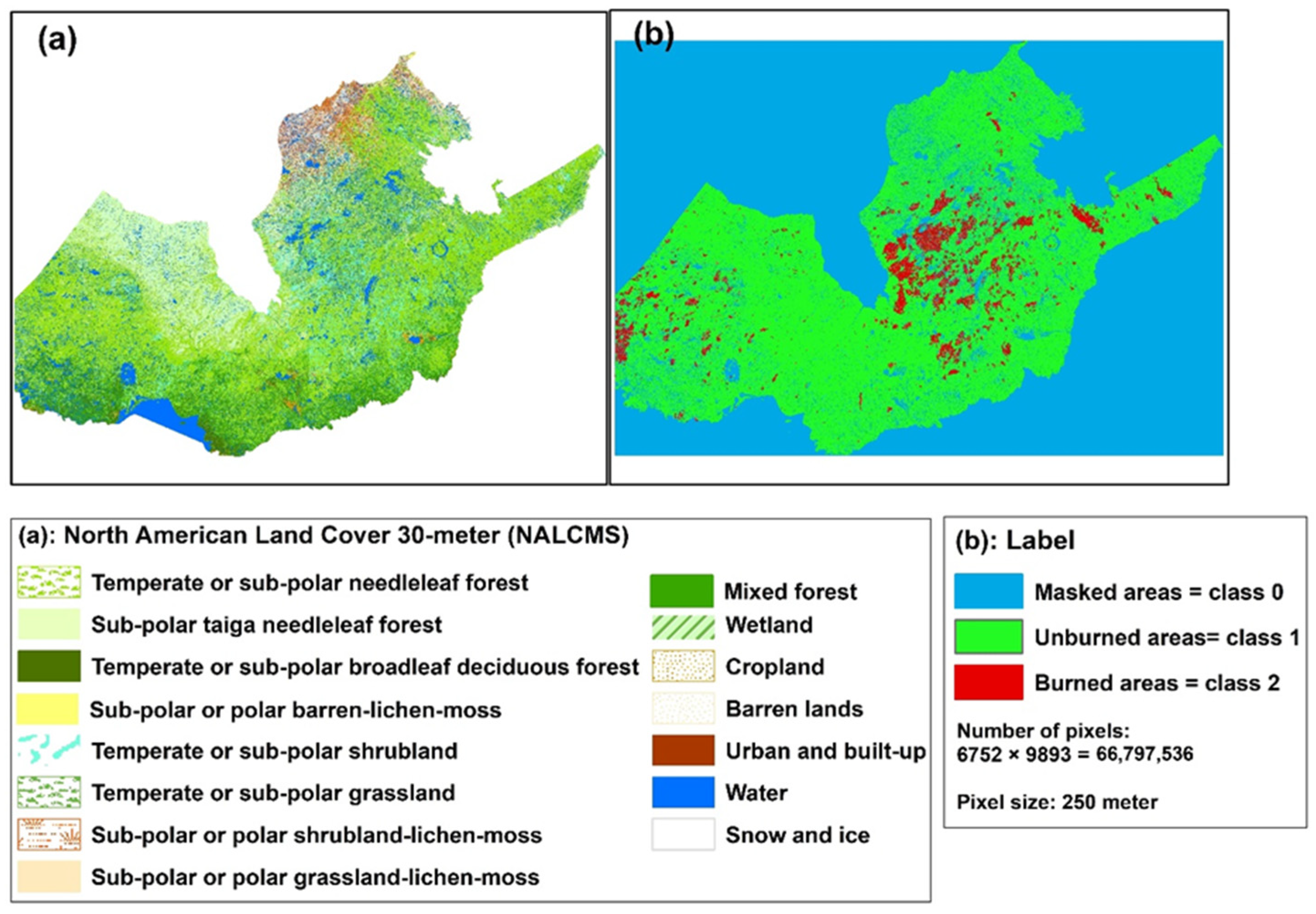
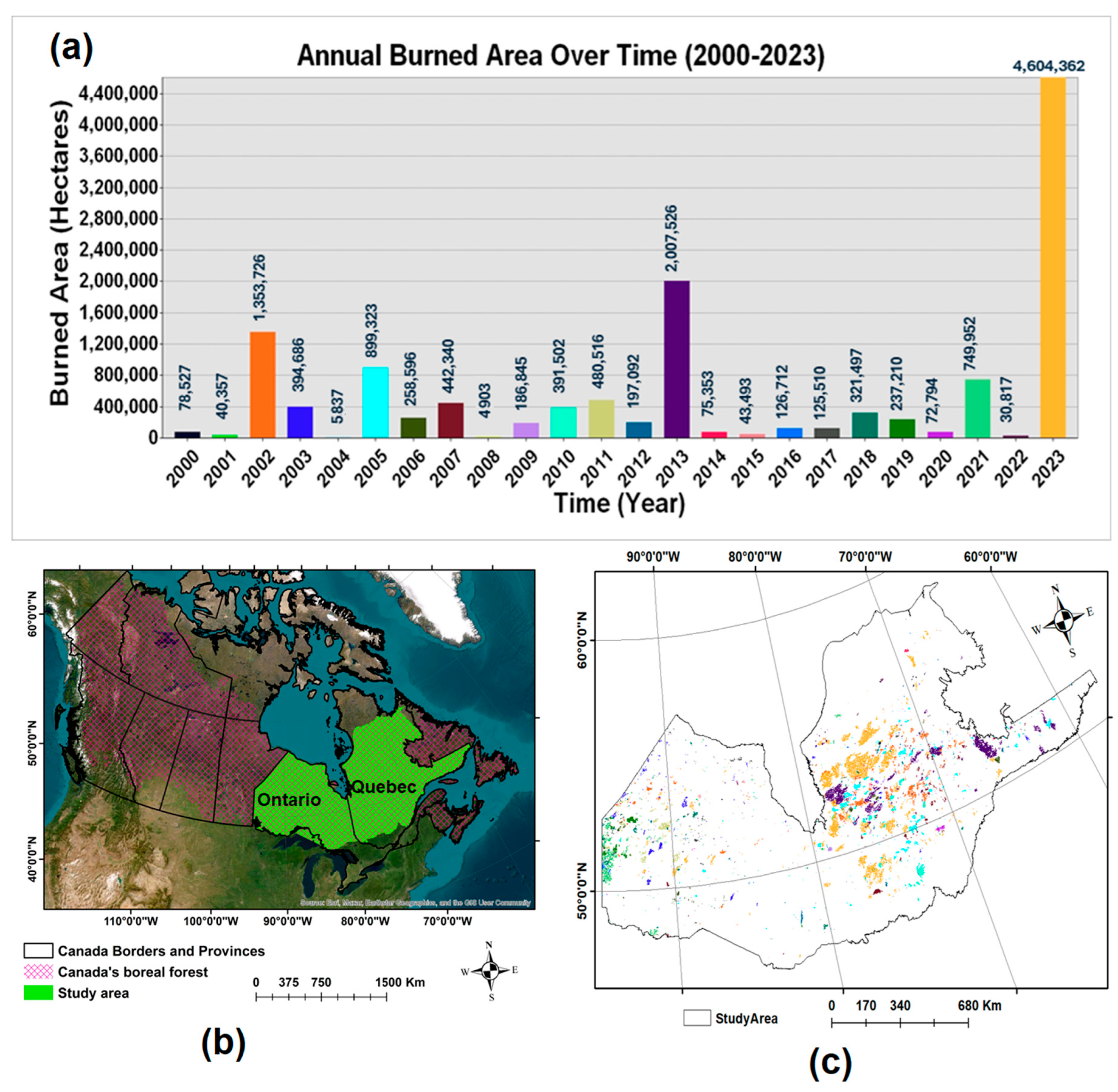
2.1. Study Area

The study area was located in the boreal forest of Eastern Canada, covering approximately 175 million hectares across the provinces of Quebec and Ontario. This region is predominantly composed of coniferous forests, including black spruce (Picea mariana), white spruce (Picea glauca), balsam fir (Abies balsamea), tamarack (Larix laricina), and jack pine (Pinus banksiana). Additionally, some broad-leaved species are present, such as trembling aspen (Populus tremuloides), large-toothed aspen (Populus grandidentata), Eastern cottonwood (Populus deltoides), white birch (Betula papyrifera), and balsam poplar (Populus balsamifera) [5]. Figure 1 illustrates the location of the study area, along with the annual total burned area from 2000 to 2023, based on data from the National Burned Area Composite of Natural Resources Canada [50].
Over this period, large wildfires have become more frequent and intense, reflecting the increasing severity of fire activity in recent decades. Notably, 2023 recorded the highest burned area (4,604,362 hectares). This accounts for approximately one-third of the total area affected by wildfires across Canada in 2023, underscoring the national significance of the study region in the national wildfire context. This trend reinforces the urgent need for improved wildfire prediction and management strategies to mitigate the ecological and economic consequences of wildfires in boreal ecosystems.

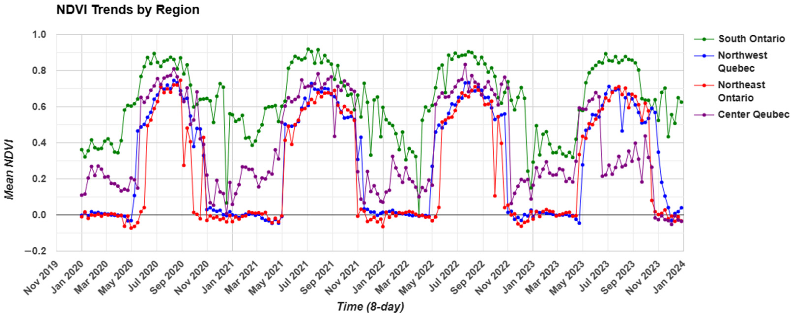
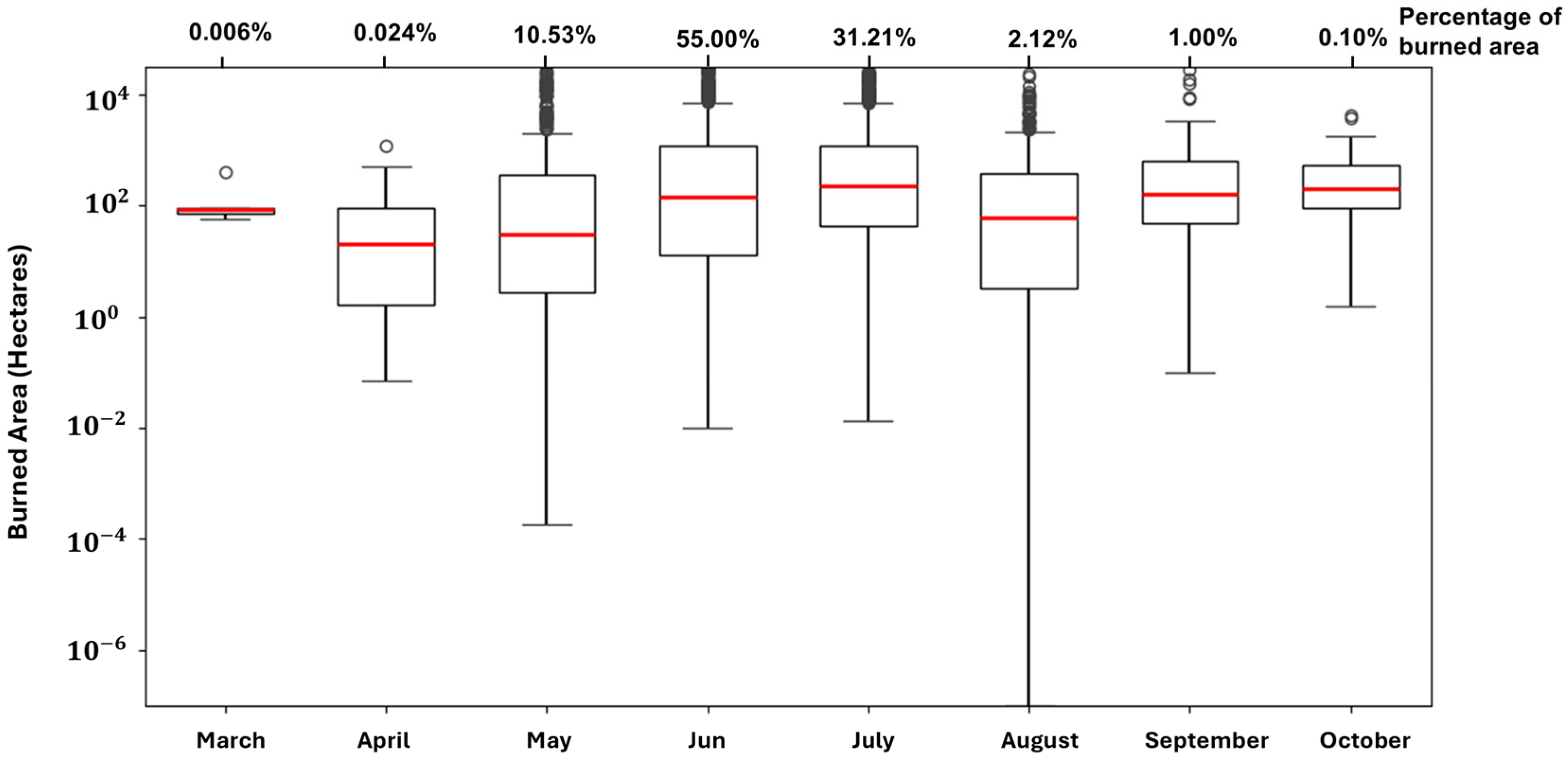
Seasonal Vegetation Dynamics and Wildfire Activity in the Eastern Canadian Boreal Forest

Research focusing on boreal ecosystems [51,52] underscores the importance of considering seasonal dynamics when assessing wildfire impacts. The selected time period from 15 June to 1 September was chosen to align with the peak growing season of the boreal forest in Canada, where vegetation is most active. Studies such as [53] have emphasized the utility of vegetation indices like the NDVI in monitoring ecological changes during active growing seasons. The trends of the mean NDVI (Figure 2) exhibit a pronounced seasonal pattern in different regions of the study area (South of Ontario, Northwest of Quebec, Northeast of Ontario, and Center of Quebec) and clearly illustrate the vegetation activity peaks during the summer months across these regions, highlighting the ecological significance of the summer period. Thus, this period (15 June–1 September) captures the maximum vegetation greenness, which is essential for accurately analyzing the effects of wildfires on vegetation [54].
Due to the substantial variation in burned area across different months, a logarithmic scale was applied to the box plot in Figure 3 to enhance visualization, allowing for a more accurate representation of the data distribution. This seasonal wildfire activity, predominantly from May to September, coincides with periods of elevated temperatures and extended dry conditions, particularly in June, July, and August. These months exhibit a broad interquartile range in burned area and a higher frequency of extreme fire events, suggesting that the hot and dry climate during this period contributes significantly to both the frequency and severity of wildfires which is overlapped with the growing season. In contrast, months such as March and October show minimal wildfire occurrence with relatively stable burned area distributions. During this period, wildfires account for over 88% of the total burned area, with June contributing 55%, followed by July (31.2%) and August (2.13%). By focusing on this critical fire season, the study ensures that wildfire activity is assessed during its most impactful period, thereby optimizing the computational efficiency and predictive accuracy. Furthermore, this targeted timeframe effectively captures vegetation changes associated with fire events, facilitating a more precise assessment of wildfire impacts on ecosystem dynamics [55,56].

2.2. Source Materials

This study employed remote sensing data from MODIS products, specifically the NDVI, LST, and SWIR, which are critical variables influencing wildfire dynamics [48]. The reflectance bands—referred to in GEE by their product-specific names as sur_refl_b01, b02, b03, and b07, corresponding to standard MODIS Bands 1, 2, 3, and 7, respectively—were obtained from the MOD13Q1 V6.1 (Terra) and MYD13Q1 V6.1 (Aqua) products in GEE. GEE allows users to efficiently search and access satellite imagery based on customizable parameters such as geographic boundaries, temporal range, and cloud cover thresholds. This functionality is particularly advantageous for studies requiring consistent and long-term temporal coverage, like those examining seasonal variations or long-term environmental trends [57]. For MODIS data, the NDVI is derived using Band 1 and Band 2 (Table 1). These bands are specifically designed to capture the variations in vegetation reflectance, where healthy vegetation absorbs red light for photosynthesis and reflects NIR light due to its internal leaf structure. In this study, NDVI values were derived from the MOD13Q1.061 (Terra) and MYD13Q1.061 (Aqua) Vegetation Indices Global datasets in GEE, calculated using Equation (1) [53]:
N D V I = N I R R E D N I R + R E D
LST values were sourced from the MOD11A1 V6.1 (Terra) and MYD11A1 V6.1 (Aqua) products within GEE. These values, originally in Kelvin, were converted to Celsius using a scaling factor (0.02) and an offset (−273.15). This conversion allowed for an intuitive interpretation of temperature data. The analysis conducted in GEE with a comprehensive spatiotemporal evaluation of LST changes, facilitates a better understanding of fire-induced thermal anomalies. Such insights are crucial for wildfire risk assessment, management, and post-fire vegetation recovery monitoring [58,59].
Data were processed for the period between 15 June and 1 September each year, corresponding to the peak wildfire and growing seasons in the boreal forests of eastern Canada, specifically in Quebec and Ontario. Initially, the datasets had different spatial resolutions of the NDVI: 250 m, Band 7: 500 m and LST: 1 km (see Table 1). To ensure consistency and facilitate analysis, Band 7 and LST datasets were resampled to a uniform spatial resolution of 250 m using bilinear interpolation in GEE, aligning it with the native resolution of the NDVI. This standardization allows for seamless integration of the variables and ensures compatibility in the subsequent processing and modeling steps.
Using the 2020 North American Land Cover 30 m dataset [60], produced as part of the North American Land Change Monitoring System (NALCMS) (see Appendix A.1, Figure A1a), non-relevant land cover types—such as water bodies, urban zones, croplands, and anthropogenic disturbances—were masked using GEE, ensuring that all the remaining areas were retained for analysis. To reduce the influence of seasonal noise and non-fire periods, data were aggregated annually using only observations from the growing season (15 June to 1 September). For each year, maximum, minimum, mean, and median values of the NDVI, LST, and Band 7 reflectance were computed within GEE to characterize the key environmental conditions associated with wildfire activity. Table 1 provides a summary of the selected features used in the model.
Annual NDVI, LST, and Band 7 metrics were generated for each year in the study period. These features served as inputs for the MLP model, with their relevance supported by previous studies demonstrating their effectiveness in wildfire detection [33]. The processed annual datasets were exported in GeoTIFF format using GEE’s export functions. Each dataset was clipped to the study area geometry and prepared for integration into the MLP model.
The overall methodology for burned area detection using a DL-based MLP model is illustrated in Figure 4. The workflow includes MODIS-derived feature extraction, land cover masking, data preprocessing, feature standardization, and classification using an MLP model. Additionally, the process incorporates hyperparameter tuning, cross-validation, and performance evaluation to optimize the model for accurate burned area detection.

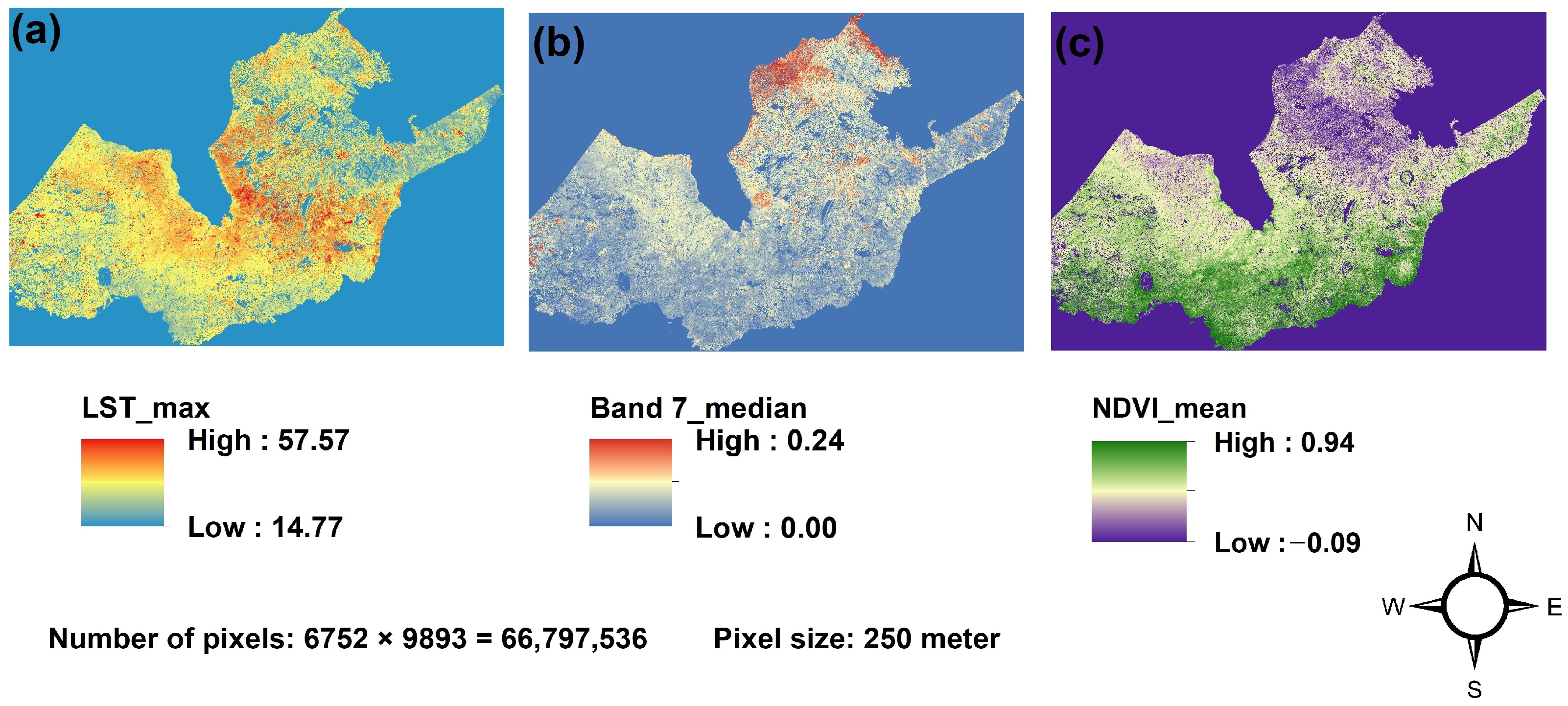
2.3. Spatial Data Extracted from the Dataset Spanning from 2000 to 2023
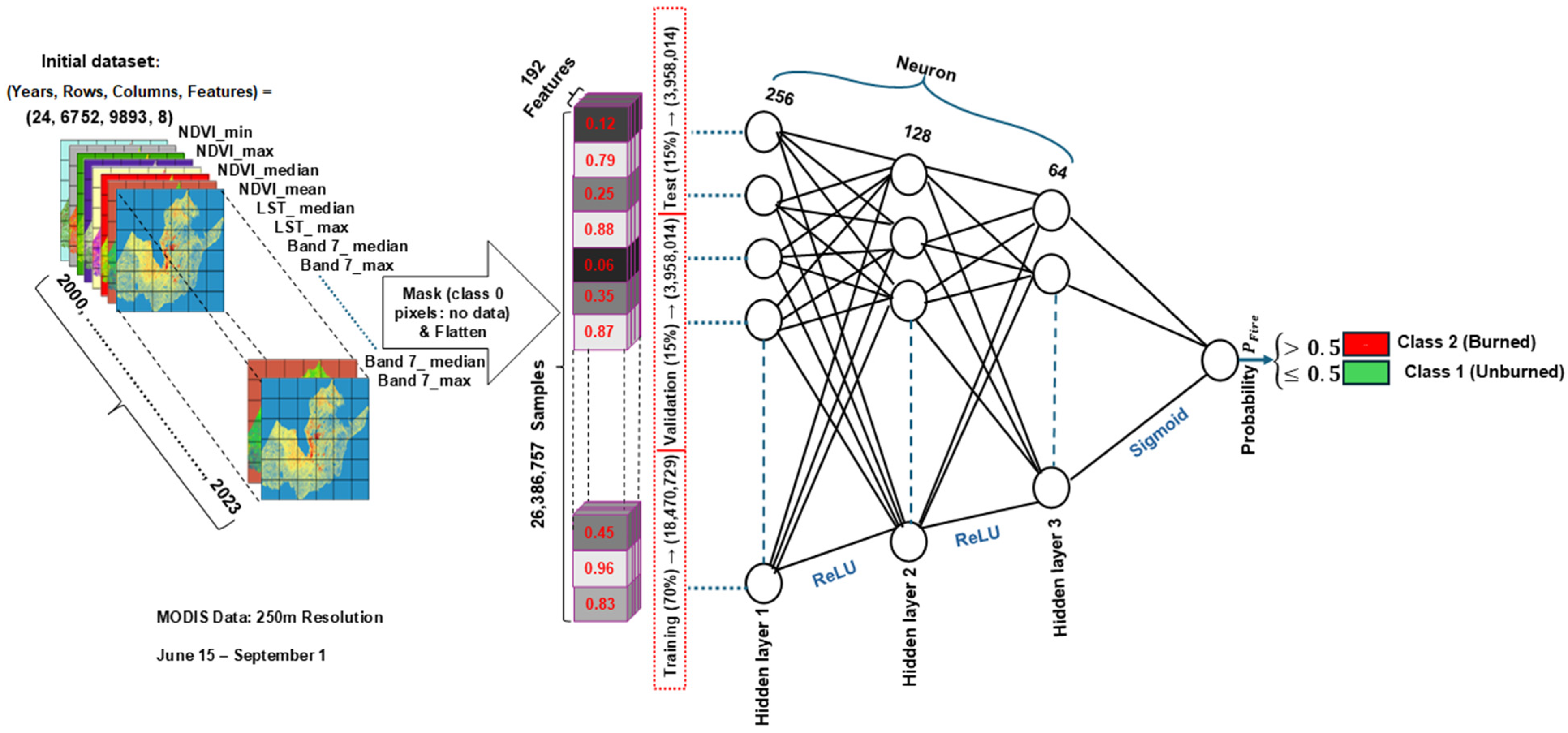
The dataset used in this study spanned the period from 2000 to 2023 and included the annual values of eight environmental features (see Table 1), derived from MODIS imagery and processed using GEE. With a spatial resolution of 250 m, the dataset comprised 66,797,536 pixels (6752 × 9893), ensuring detailed spatial coverage across the study region. Figure 5 illustrates a representative subset of this dataset using sample data from the year 2020. Selected features—LST_max, B7_median, and NDVI_mean—are shown to demonstrate the environmental variability and spatial gradients captured by the dataset.
The spatial distribution of labels used for the DL classification in this study was derived from merged burned area data spanning from 2000 to 2023 (Figure 1 and Figure A1b in the Appendix A.1). Rasterization was performed using the rasterio.mask.mask function in Python (version 3.12), which masked wildfire shapefiles based on their spatial geometry. This process produced raster labels where unburned areas were assigned a value of 1 (green), burned areas a value of 2 (red) and non-relevant regions a value of 0 (blue). The final raster labels were saved as GeoTIFF files, with georeferencing information—including the affine transformation and coordinate reference system (CRS)—preserved. The CRS was explicitly set to NAD83/Canada Atlas Lambert, ensuring spatial consistency with the input features. After masking out irrelevant pixels, the final study area contained 26,926,757 pixels. Among these, 24,504,452 pixels (91%) were classified as unburned areas (Class 1), while 1,882,305 pixels (9.0%) represented burned areas (Class 2). This distribution reflects the spatial extent of wildfire activity within the region and highlights the class imbalance in the dataset, which was accounted for in subsequent modeling and analysis.

2.4. Preprocessing

The dataset preparation for developing the burned area detection model involved a series of preprocessing steps to ensure data consistency and quality. To address missing data in the feature set, a systematic gap-filling approach was implemented. The presence of missing or undefined values in the dataset arose due to various factors, including sensor limitations, cloud cover, and atmospheric interference—common issues in remote sensing data acquisition [61]. Since DL models such as MLP models require complete datasets for effective learning, handling missing data was a critical preprocessing step [33]. For pixels categorized as class 1 (unburned) and class 2 (burned), missing values were replaced with the temporal mean of that pixel across all available years. This method ensured that the replacement value retained the trend over the study period for that specific pixel rather than introducing values from other locations. This is particularly important in wildfire modeling, where land surface characteristics (e.g., NDVI, LST, Band 7) can vary significantly across space but tend to follow temporal patterns at specific locations. In cases where a pixel had missing values in all years (i.e., there were no valid data for that location in the period time), a mean for the corresponding feature was computed from all the available valid pixels in the dataset. Using the above mean values as a fallback ensured that no empty values remained in the feature set, thereby preventing computational errors during model training. Specifically, the fallback was applied to 268,441 pixels for the LST, 29,747 pixels for the NDVI, and 29,312 pixels for Band 7.
To standardize the feature values, min–max normalization was applied independently to each feature across all years and all pixels. This process scaled all the feature values to a range of [0, 1], using Equation (2) [62], improving the stability and performance of the MLP model.
X = X X m i n X m a x X m i n
where X = original data value of a feature; X m i n = minimum value of the feature; X m a x = maximum value of the feature; X = scaled data value.
This transformation ensured that all features contributed equally during model training by normalizing their numerical ranges, which improved the numerical stability and convergence for ML and DL models while preserving the relative structure of the data [63]. This workflow ensured that the input data were normalized, masked, and spatially consistent, ready for burned area detection tasks.
After normalization, the data were reshaped into a flat format suitable for input into the MLP model. Pixels labeled as class 0 were masked to exclude non-relevant areas from further analysis, aligning with previous studies emphasizing the importance of excluding such areas in wildfire modeling [64], and the remaining valid pixels (Classes 1 and 2) were flattened to create structured arrays suitable for model input. The final feature matrix contained 192 values per sample (8 features × 24 years). The dataset was divided into training (70%), validation (15%), and testing (15%) subsets using a stratified split to maintain the proportional distribution of burned and unburned pixels [65]. This approach ensured that each subset adequately represented the data variability, supporting effective model training and evaluation. An overview of this preprocessing pipeline is illustrated in Figure 6.

2.5. Model Selection and Performance Evaluation (2016–2018)

Before applying the model to the entire study period (2000–2023), an initial evaluation was conducted on a subset of both the study area and study period (2016–2018) to identify the most effective machine learning model for wildfire detection. This period was selected randomly from recent years and provided a manageable yet representative dataset in terms of both burned and unburned areas. Due to computational constraints associated with the full dataset, this preliminary phase allowed for rapid model comparison and tuning before full-scale implementation. To ensure comprehensive representation of wildfire activity, all burned pixels from the 2016–2018 period were included, while a stratified sample of unburned pixels was drawn at a 5:1 unburned-to-burned ratio, following the approach used by [66]. This sampling strategy ensured that wildfire-affected areas were fully represented while maintaining a balanced and computationally efficient dataset. To compare the model performance, three machine learning models—Multilayer Perceptron (MLP), Support Vector Machine (SVM), and Random Forest (RF)—were trained using this subset. Each pixel was represented by eight features derived from the NDVI, LST, and Band 7 (maximum, minimum, mean, and median values). All the models were trained using default hyperparameters, as summarized in Appendix A.5, to enable consistent comparison prior to full hyperparameter tuning.

2.6. Training and Hyperparameter Tuning of the Multilayer Perceptron (MLP) Model

The MLP model, a feedforward artificial neural network [67], was selected for this study due to its capacity to learn complex, non-linear patterns, making it well-suited for burned area detection [68], where features such as the NDVI, Band 7, and LST exhibit non-linear relationships. To effectively develop and optimize the MLP model, a systematic workflow was implemented, including hyperparameter tuning, model training, and validation. The training and validation datasets, preprocessed and stored as NumPy arrays, contained essential features designed to capture patterns indicative of burned areas during the growing season. Labels representing burned and unburned pixels were included to facilitate supervised learning, while preprocessing ensured computational efficiency and data integrity. The MLP architecture consists of an input layer, three hidden layers, and an output layer (Figure 6).
The input layer processes the selected features, while the hidden layers transform inputs into abstract representations by applying weights ( w ) and biases ( b ) , adjusted during training using backpropagation and stochastic gradient descent. For a specific layer l + 1 , the output activation a ( l + 1 ) is calculated using Equation (3) [66,69]:
a ( l + 1 ) = f w ( l ) a ( l ) + b ( l ) )
where f denotes the nonlinear activation function, such as ReLU, and a ( l ) represents the activation of the previous layer. For a given set of input features x , the output of the MLP model ( h w , b ( x ) ) is expressed as:
h w , b x = a ( m )
where m is the number of layers in the network. The learning objective is to minimize the difference between the predicted outputs h w , b x and the true labels ( y ) , achieved by minimizing the mean squared error:
J w , b ; x , y = 1 2 h w , b x y 2 .
In this study, the output layer consisted of a single neuron with a sigmoid activation function, designed to detect burned areas by estimating the probability that a given pixel is burned. Pixels with probabilities greater than 0.5 were classified as burned (class 2), while those below this threshold were classified as unburned (class 1). This architecture allowed the MLP model to capture complex nonlinear relationships among the input features, resulting in accurate pixel-level burned area detection [66,70].

2.6.1. Hyperparameter Tuning and Selection

Hyperparameter optimization plays a crucial role in enhancing the performance of ML and DL models, particularly Multi-Layer Perceptrons (MLPs) [71]. Selecting the number of hidden layers and neurons in a neural network remains a challenging task without an exact solution, especially in remote sensing applications. While a single hidden layer can theoretically approximate continuous functions, practical applications often require deeper architectures to enhance accuracy and efficiency. To systematically identify the best architecture, GridSearchCV was used for hyperparameter tuning, evaluating all possible combinations within a predefined search space [72]. The hyperparameter grid included three hidden layer configurations—(128, 64, 32), (256, 128, 64), and (64, 32)—chosen to balance model capacity and computational efficiency. These configurations align with remote sensing best practices, where multi-layer architectures effectively capture complex spatial patterns while mitigating overfitting and computational costs [73,74]. The systematic reduction in neurons across layers enhances hierarchical feature learning, making these configurations [75] particularly well-suited for burned area detection tasks.
The ReLU activation function was selected for its efficiency and ability to prevent vanishing gradients, making it well-suited for large-scale wildfire detection [76]. L2 regularization was applied to reduce overfitting, with strengths (α = [0.0001, 0.001, 0.01]) tested during tuning [73]. Both SGD [77] and Adam [78] optimizers were evaluated to ensure flexible and stable convergence. Hyperparameter combinations were assessed using the F1-score for burned pixels and Cohen’s kappa to ensure balanced and robust classification performance [79]. This comprehensive exploration (Table 2) of the hyperparameter space ensured the selection of an optimal MLP architecture tailored to the specific dataset and burned area detection. The best-performing model was then identified and used for further analysis in cross-validation.

2.6.2. Cross-Validation for Evaluating Model Robustness and Performance on Unseen Test Data

Cross-validation is a crucial step in ML and DL workflows to assess the robustness and generalization capabilities of a model [80]. It involves partitioning the dataset into multiple subsets (folds) and iteratively training and validating the model on different data splits. This method ensures that the model’s performance is evaluated comprehensively across various data subsets, reducing the risk of overfitting and providing a reliable estimate of its effectiveness [81,82]. In this study, a Stratified K-fold cross-validation approach was employed with five folds (n_splits = 5). This method ensures that the class distribution is preserved in both training and validation datasets within each fold, which is particularly important for imbalanced datasets like burned area detection [83,84]. Prior to cross-validation, the original dataset was randomly divided into three subsets: training (70%), validation (15%), and testing (15%). The initial training and validation sets were used for model tuning and hyperparameter selection. After tuning, the training and validation sets were merged and divided into five stratified folds for cross-validation. In each fold, 85% of the combined dataset was used for training and 15% for validation. This process was repeated five times, ensuring that each fold served as the validation set once. After ensuring the robustness and generalization of the MLP model through cross-validation, the model was evaluated on an unseen test dataset to assess its predictive performance.

2.7. Assessment of MLP Model Performance

The performance of the MLP model was evaluated using a range of statistical metrics to assess its accuracy and effectiveness in wildfire prediction. These metrics included overall accuracy, precision, recall, F1-score, Macro Average, weighted average and Cohen’s kappa coefficient. Each metric provided a unique perspective on the model’s performance, addressing challenges posed by class imbalance and the spatial complexity of wildfire occurrences [38,45,85]. Given the class imbalance, particular attention was given to the F1-score for the burned class and the Kappa coefficient, both of which provide a more balanced assessment of the model’s effectiveness. These metrics collectively offered a comprehensive evaluation of the model’s ability to detect the burned areas in unseen data [86]. Table A1 presents the confusion matrix, and the corresponding explanation is provided in Appendix A.2.

3. Results

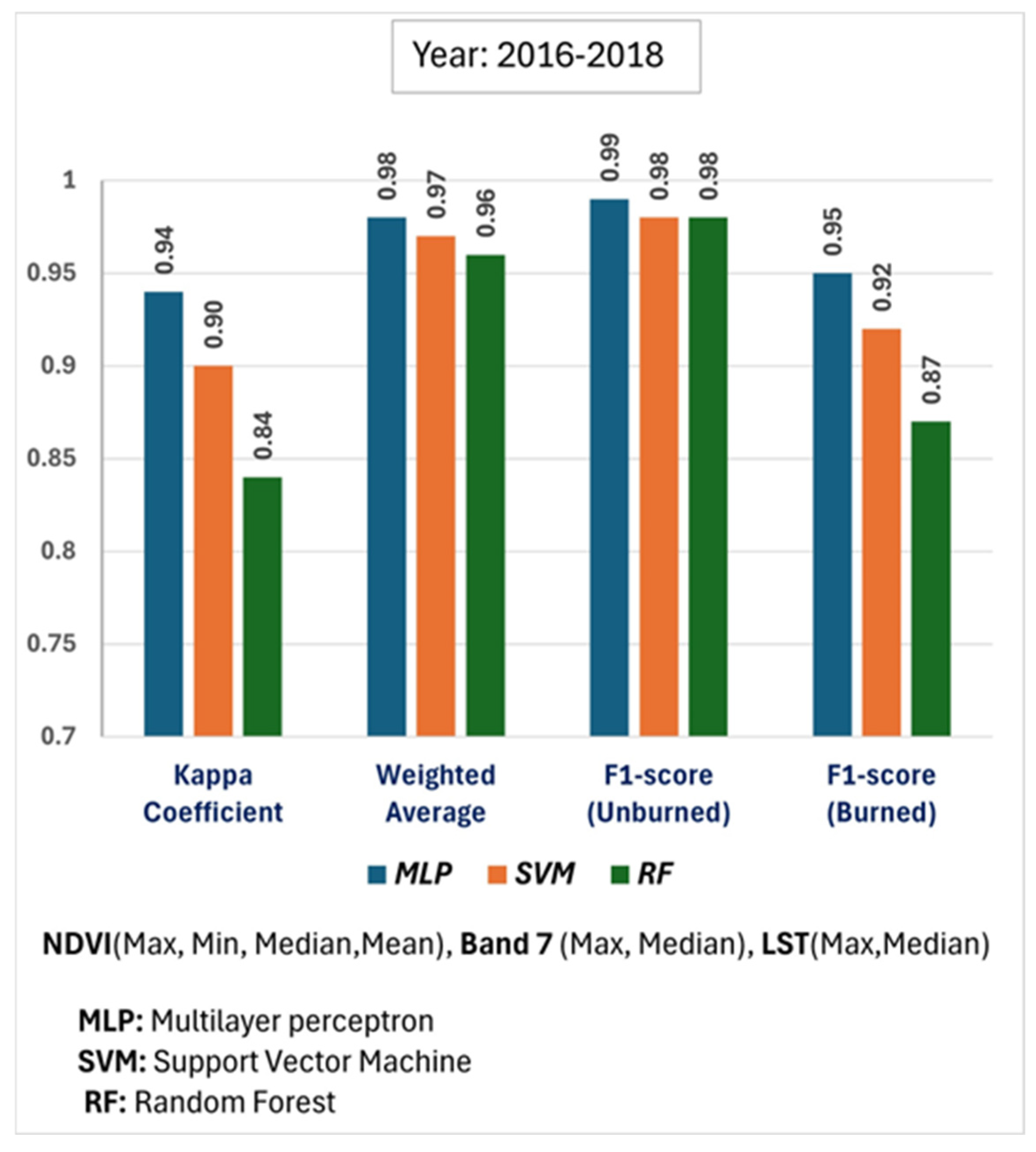
3.1. Comparative Model Performance (2016–2018)

3.1.1. Comparison of Performance Metrics Across Machine Learning Models

To compare the effectiveness of the models, we evaluated their performance using key metrics. Figure 7 illustrates the accuracy metrics for each model, showing that the MLP consistently outperformed SVM and RF across all the evaluation criteria. Although more computationally demanding than SVM and RF, the MLP model achieved higher classification accuracy—particularly for burned pixels—making it well-suited for burned area detection tasks where accuracy is prioritized over processing speed.
It achieved the highest Kappa coefficient (0.94), significantly outperforming SVM (0.90) and RF (0.84), indicating stronger agreement between predictions and actual labels. Additionally, the weighted average F1-score for MLP was 0.98, compared to 0.97 for SVM and 0.96 for RF, highlighting its superior generalization across classes. When focusing on classification, MLP achieved the highest F1-score for burned areas (0.95), outperforming SVM (0.92) and RF (0.87). Similarly, for unburned areas, all three models performed comparably, with F1-scores above 0.97. The superior performance of MLP can be attributed to its ability to capture non-linear relationships and adapt to high-dimensional input features. These findings align with [74], who also reported MLP’s superiority over other models in predicting forest fires, further supporting its effectiveness for burned area detection.

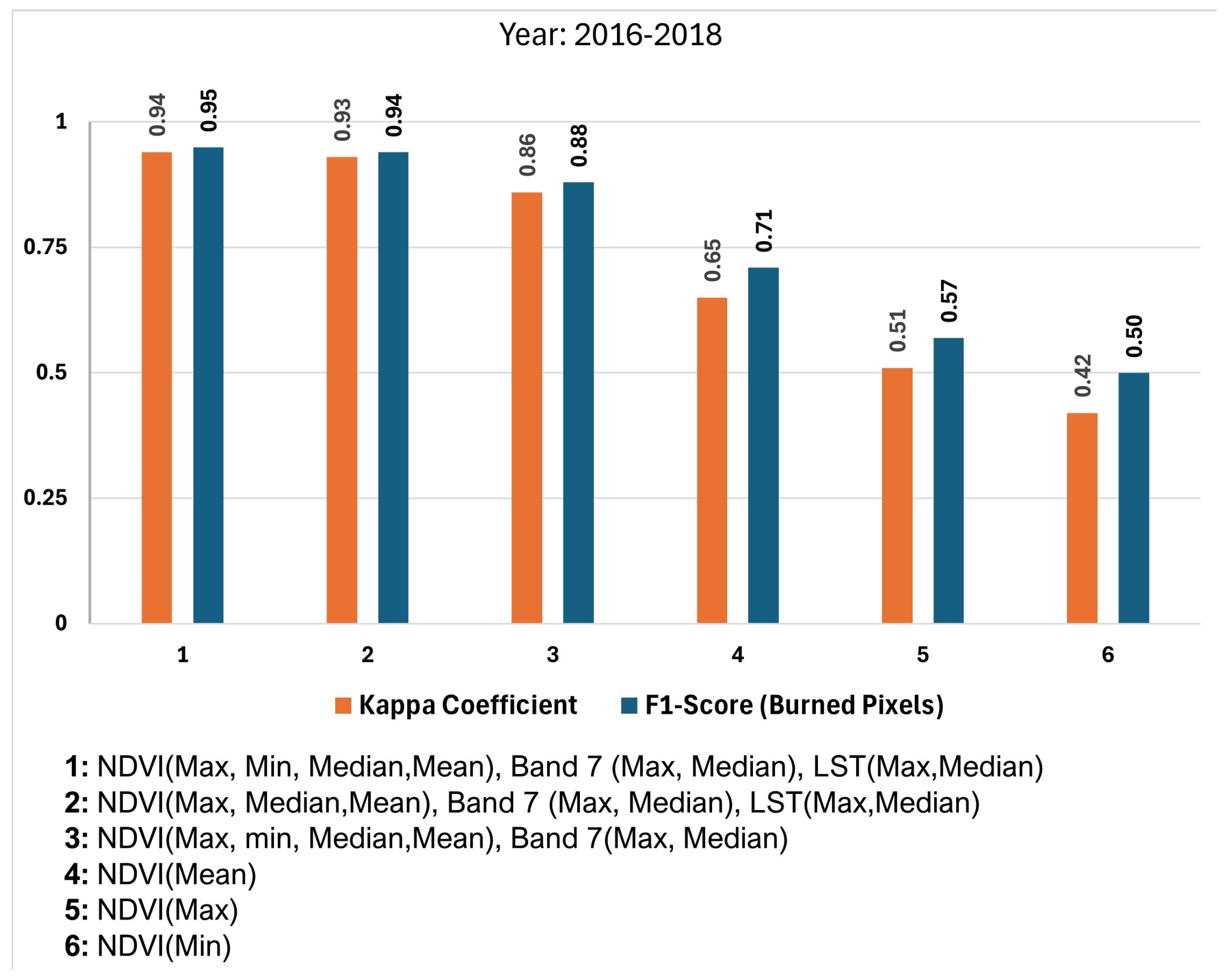
3.1.2. The Importance of Combining Multiple Biophysical Indicators for Accurate Burned Area Detection

The MLP model, using default hyperparameter settings, was included in the comparative analysis to assess its effectiveness in burned area classification. As illustrated in Figure 8, the analysis evaluated the burned area detection performance for the years 2016–2018, demonstrating the superior performance of models that incorporate a combination of the NDVI, Band 7, and LST metrics over models relying on individual features. The figure assesses six feature sets, progressively removing indicators to analyze their impact on classification performance. The first category (All Features) includes NDVI (Max, Min, Median, Mean), Band 7 (Max, Median), and LST (Max, Median), achieving the highest Kappa coefficient (0.94) and F1-score for burned pixels (0.95). The second category, which removes NDVI_min and retains the other seven features, exhibits a slight decrease in performance (Kappa: 0.93, F1-score: 0.94), indicating that NDVI_min contributes less significantly to burned area classification for this period. A more noticeable decline is observed in the third category, where LST is removed, leaving only the NDVI and Band 7. The performance drops to (Kappa: 0.86, F1-score: 0.88), emphasizing the importance of thermal data (LST) in burned area detection. The fourth category, which isolates NDVI_mean as the sole feature, shows a further decline (Kappa: 0.65, F1-score: 0.71), demonstrating that using only an annual mean of vegetation index is insufficient for reliable classification. The last two categories analyze NDVI_max and NDVI_min individually, with both performing significantly worse (Kappa: 0.51 and 0.42, F1-score: 0.57 and 0.50, respectively), confirming that a single vegetation indicator does not provide enough discriminative power for burned area detection. Given the computational constraints, selecting only the Max and Median values for Band 7 and LST optimizes efficiency while retaining the most relevant wildfire indicators. Overall, Figure 8 reveals that feature reduction progressively weakens the classification performance over the 2016–2018 period, reinforcing the necessity of integrating multiple biophysical indicators for accurate and robust burned area detection.

3.2. MLP Model Performance and Evaluation Across the Entire Study Area and Study Period (2000–2023)

Min-max normalization was applied to all eight environmental features, rescaling their values to a standardized range of 0 to 1 while preserving their original distribution and variability. A visualization of this normalization process for three representative features (LST_max, B7_median, and NDVI_mean) is provided in Appendix A.3 Figure A2. The results of the model tuning configurations are summarized in Table 3, ranked according to Cohen’s kappa and F1-score (Burned Pixels). Among the tested configurations, Tuning 14 achieved the best performance, with a Cohen’s kappa of 0.8890 and an F1-score of 0.90. This configuration utilized a network architecture with three hidden layers [(256, 128, 64)], the SGD optimizer, and a regularization parameter (α) of 0.0001. Close behind, Tuning 15 also showed excellent performance (kappa = 0.8847, F1-score = 0.89) with the same architecture and optimizer but a higher regularization (α = 0.001). Configurations Tuning 11 and Tuning 12 ranked third and fourth, respectively, maintaining competitive performance with slightly smaller hidden layer sizes [(128, 64, 32)] and similar regularization settings. The results highlight that the SGD optimizer, combined with appropriately chosen regularization, outperformed configurations using the Adam optimizer. Notably, the top-performing configurations used deeper architectures with larger hidden layer sizes [(256, 128, 64)], suggesting that more complex models were effective in capturing the underlying patterns in the data. In contrast, configurations with shallower architectures [(64, 32)] or higher regularization (α = 0.01) demonstrated lower performance, as observed in the rankings of Tuning 16 and below. These findings underscore the importance of optimizing both the network architecture and regularization parameters to achieve robust wildfire prediction based on burned pixel classification.
To evaluate the robustness and generalizability of the burned area detection model, a five-fold cross-validation was conducted. The model demonstrated consistent performance across all folds, with Cohen’s kappa values ranging from 0.8834 to 0.8862, reflecting excellent agreement beyond chance. This consistency indicates the model’s reliability in correctly distinguishing between burned and unburned areas. Additionally, the F1-score for the burned class (Class 2) remained stable at 0.89 across all folds, further showcasing the model’s robustness in identifying burned pixels despite the significant class imbalance. These metrics highlight the effectiveness of the proposed MLP architecture in addressing the challenges of burned area detection.
A comprehensive evaluation of the final model’s performance on the test data was conducted using multiple metrics, as detailed in Table 4. The model achieved a Cohen’s kappa value of 0.8839, indicating strong agreement between predictions and actual labels beyond chance. The overall accuracy was 0.9846, reflecting the model’s high capability in correctly classifying both burned and unburned pixels. For individual class performance, Class 2 (burned areas), which is of primary interest, had an F1-score of 0.89, with precision and recall both at 0.89, indicating reliable performance in detecting wildfire-affected areas despite class imbalance. Additionally, the macro-average F1-score was 0.94, reflecting the model’s balanced performance across both classes, while the weighted average F1-score was 0.98, confirming the overall strong predictive capability of the model. These results, as shown in Table 4, validate the model’s robustness, ensuring both high sensitivity in detecting burned pixels and strong generalization across the dataset.

4. Discussion

4.1. Comparative Analysis of the MLP Model for Burned Area Detection

The proposed MLP model achieved a Cohen’s kappa of 0.8839 and an F1-score of 0.89 for burned pixels, demonstrating competitive performance compared to other state-of-the-art DL architectures for burned area detection. For instance, U-Net achieved kappa coefficients as high as 90% on Sentinel-2 data in Mediterranean fire sites [39], while Burnt-Net reported accuracies up to 98.08% on post-fire Sentinel-2 images [43]. Similarly, BA-Net achieved a Dice coefficient of 92% using datasets from multiple regions [34].
By focusing on computational efficiency, the MLP model achieves a strong balance between simplicity and predictive power. It outperforms simpler architectures like CNNs [47] and hybrid unsupervised methods [87] while maintaining scalability. Fast-SCNN achieved a kappa coefficient of over 79% in a compact boreal forest fire site in Sweden [39], whereas our MLP model achieved a higher kappa of 88% without relying on high-resolution spatial features. Likewise, hybrid unsupervised methods such as in [87], which utilized VGG16-based feature extraction and achieved an F1-score of 87%, were comparable to our MLP model. The computational efficiency of the MLP model becomes particularly critical when scaling to large regions, such as the boreal forest of eastern Canada, which includes over 66 million pixels.
Deep learning architectures like U-Net [40,44] and Burnt-Net [43] depend on high-resolution datasets such as Sentinel-2 and Landsat-8. For instance, U-Net achieved F1-scores ranging from 91.8% to 93.8% using PlanetScope imagery (3 m resolution) [44] and 82% to 92% on Sentinel-2 (10 m resolution) data in Central Africa and Indonesia [42]. While these models excel in detecting fine-grained spatial patterns, their scalability is constrained by the computational burden of high-resolution imagery and deep architectures. In contrast, the MLP model, by focusing on coarse-resolution MODIS data, provides a scalable and efficient alternative for burned area detection, achieving competitive accuracy with substantially lower computational requirements.
Additionally, the MLP model compares favorably with recent DL architectures such as deep residual U-Net and BA-Net. Deep residual U-Net achieved F1-scores of 78.07% and 84.23% on the Chuckegg Creek and Sydney fire datasets, respectively [65], while BA-Net attained a Dice coefficient of 92% across multiple regions [34]. Furthermore, DSMNN-Net demonstrated high accuracies of 90.24% and 97.46% using pre- and post-fire Sentinel-2 and PRISMA datasets [41]. However, these models rely on high-resolution imagery, 3D convolutional layers, encoder–decoder structures, transposed convolutions, and morphological operations, all of which are computationally expensive and require large-scale datasets with advanced spatiotemporal processing. By contrast, the MLP model does not depend on pre- and post-fire imagery but instead utilizes annual aggregated features, providing a more efficient and scalable approach for burned area detection across large regions. This trade-off between spatial resolution and computational efficiency highlights the versatility of the MLP model, which effectively processes coarse-resolution data while maintaining strong predictive accuracy.
Unlike CNN-based architectures, which automatically learn spatial features from high-resolution images, the MLP model relies on feature engineering to extract meaningful wildfire-related patterns. By aggregating annual MODIS-derived features, the model ensures the inclusion of critical variables while minimizing data noise and redundancy. Effective preprocessing and feature selection played a crucial role in optimizing the model’s performance. Studies such as [39,87] have demonstrated that feature extraction techniques (e.g., VGG16) and preprocessing methods (e.g., GLCM dissimilarity, topographic normalization) can significantly enhance the model accuracy.

4.2. Selecting Statistical Metrics (Max, Min, Mean, Median) for the MLP Model in Burned Area Detection

Statistical metrics such as maximum, minimum, mean, and median were chosen for features like the NDVI, Band 7, and LST to capture the temporal and spatial variability essential for burned area detection. These metrics summarize the key aspects of vegetation and surface conditions, which are critical factors influencing wildfire areas. Maximum and minimum values provide insights into the extremes of vegetation health and surface reflectance or temperature. For example, maximum NDVI values are commonly associated with peak vegetation greenness, while maximum LST reflects surface heating hotspots often associated with fire activity. Minimum values highlight areas of stressed vegetation or cooler surface conditions. Mean values capture the overall conditions across the growing season, offering a general understanding of vegetation and temperature dynamics that contribute to wildfire. Median values reduce the influence of short-term anomalies, such as those caused by clouds or sensor noise, while preserving important biological signals like partial burns. This balance ensures that the MLP model receives a robust yet ecologically meaningful representation of the landscape, aiding in distinguishing between burned and unburned areas. These metrics provide complementary information, helping the MLP model to effectively distinguish between burned and unburned areas. Our experimental results (Section 3.1.2, Figure 8) confirm the practical value of this multi-metric approach. Models that integrated all statistical summaries—the NDVI (Max, Min, Mean, Median), Band 7 (Max, Median), and LST (Max, Median)—achieved the highest performance, with a kappa coefficient of 0.94 and F1-score of 0.95 for burned pixels. As features were progressively removed, especially the LST and NDVI_min, the performance declined, reinforcing the importance of thermal and spectral variability in fire detection. Models using only a single NDVI metric (e.g., mean, max, or min) performed significantly worse, confirming that no single indicator adequately captures the complex spatial–temporal signals of burned areas. These findings highlight that the combination of extreme values (max/min) and central tendencies (mean/median) enables the MLP model to more accurately distinguish between burned and unburned pixels, while maintaining robustness against seasonal anomalies or sensor noise. This observation aligns with [88], who demonstrated that changes in the mean, minimum, and maximum values of the NDVI and LST effectively captured fire-induced vegetation loss and surface temperature rise. Their analysis confirmed that these statistical summaries are ecologically informative and useful for monitoring both the immediate fire impact and long-term forest regeneration. Similar approaches have been used in biomass estimation, where statistical summaries like max, min, and mean NDVI were shown to improve the model accuracy by highlighting key environmental patterns [89].

4.3. Limitations and Future Research Directions

Despite the strong performance of the proposed MLP model in burned area detection, several limitations remain. In particular, the Canadian National Fire Database (CNFDB) may contain missing or inaccurate records—especially for smaller or unreported fire events—introducing uncertainty into the training labels. Additionally, MODIS spatial resolution imposes constraints that hinder the detection of small fires. As illustrated in Figure 9a, 99.69% of the total burned area is attributed to large fires (>100 ha), while small-to-medium fires (<100 ha), though frequent (1656 occurrences), contribute negligibly to the total burned area. This underdetection stems from the mixed-pixel problem, where burned and unburned surfaces within a single pixel reduce the spectral contrast. Figure 9b further emphasizes the detection bias, showing that despite their frequency, smaller fires are systematically underrepresented in MODIS-derived burned area estimates. To address these challenges, future research can incorporate higher-resolution satellite data such as Sentinel-2 (10 m) or Landsat (30 m) to better capture fine-scale fire disturbances. Integrating radar data from Sentinel-1 may also help overcome cloud cover limitations in optical imagery.
A key limitation of the MLP model lies in the severe class imbalance, where unburned pixels dominate the dataset—accounting for 91% (24.5 million pixels), while burned pixels represent only 9% (1.88 million pixels). In some years, like 2000, the imbalance was even more pronounced, with only 11,477 burned compared to over 26 million unburned pixels (see Appendix A.4, Table A2). Although the model performed well (F1-score: 0.89, Kappa: 0.8839), such imbalance may reduce its sensitivity to rare fire events. Additionally, the model does not explicitly account for spatial or temporal dependencies; while yearly MODIS-derived metrics are efficient, they do not capture evolving fire patterns over time. To address this, future work could adopt a year-specific sampling strategy: retain all burned pixels from each year and randomly sample unburned pixels to ensure spatial diversity without overlap. This approach allows the model to learn the fire behavior specific to each year—capturing variations in climate, vegetation, and fire dynamics—while avoiding overfitting to repeated regions. It also preserves temporal consistency and improves generalizability. Moreover, standard techniques such as class weighting, oversampling, or cost-sensitive learning can be combined with this per-year strategy to further enhance the model robustness. Comparing this approach with the current combined-label method may reveal improvements in burned area detection accuracy and consistency across years. In addition, advanced deep learning models such as Recurrent Neural Networks (RNNs), Long Short-Term Memory (LSTM) networks [90], and Convolutional Long Short-Term Memory (ConvLSTM) networks [91] have demonstrated strong capabilities in modeling time series data related to wildfire occurrence, progression, and severity. These models are particularly promising for burned area detection when class imbalance issues are adequately addressed. Among them, ConvLSTM models—which combine the spatial feature extraction power of Convolutional Neural Networks (CNNs) with the temporal learning capability of LSTMs—have shown superior performance in fire danger forecasting using time series data. Additionally, hybrid architectures such as CNN2D-LSTM have achieved notable success in predicting global wildfires by leveraging multi-year satellite-based predictors [91].
In addition to model selection, feature engineering plays a crucial role in enhancing the accuracy of burned area detection. Ref. [92] demonstrated that novel feature indices, such as COSI1 and COSI2, significantly improved the estimation of above-ground biomass (AGB) by integrating spectral and structural information from multi-source remote sensing data. These indices reduced the information redundancy and enhanced the predictive performance. Similarly, applying feature engineering techniques like COSI1 (multiplicative combination of spectral and SAR features) and COSI2 (normalized difference of SAR and optical indices) could strengthen burned area detection models by capturing both vegetation conditions and fire-induced structural changes. Such methods are essential for improving the robustness of burned area classification, particularly in fire-prone and heterogeneous landscapes.
By integrating these advancements, future burned area prediction models can achieve higher accuracy, improved small fire detection, and enhanced temporal forecasting, ultimately contributing to more effective wildfire monitoring, management, and mitigation strategies.

5. Conclusions

This study evaluated the effectiveness of an MLP model for burned area detection in the boreal forests of eastern Canada using MODIS-derived features. The key findings are summarized as follows:
  • Superior classification performance: The MLP model consistently outperformed Support Vector Machine (SVM) and Random Forest (RF) classifiers in detecting burned areas, even under conditions of significant class imbalance.
  • Multi-source feature integration: Combining biophysical indicators—the NDVI, Band 7, and LST—led to substantially higher classification accuracy than using individual features alone, highlighting the importance of integrating vegetation, spectral, and thermal data.
  • Model optimization: Careful feature selection, hyperparameter tuning, and the use of deeper architectures with appropriate regularization contributed to improved model stability and predictive performance.
  • Generalizability: The model demonstrated consistent and reliable performance across five-fold cross-validation, confirming its applicability for operational burned area mapping.
  • Limitations: The 250 m spatial resolution of MODIS may restrict the detection of small fire events or fine-scale burn patterns. Additionally, the MLP model lacks inherent temporal modeling capabilities.
  • Future research: Subsequent studies should explore temporal deep learning architectures such as Long Short-Term Memory (LSTM) or Convolutional LSTM (ConvLSTM) to capture dynamic wildfire behavior. Incorporating data from additional sensors such as Sentinel-1 SAR may further improve the detection accuracy, particularly in cloud-prone areas.
Overall, the results demonstrate that accurate and robust burned area detection requires both comprehensive feature integration and a well-optimized model design.

Author Contributions

Conceptualization, H.M.M. and C.P.; methodology, H.M.M., M.B. and C.P.; software, H.M.M. and M.B.; formal analysis, H.M.M., M.B., C.P., J.C. and D.K.; data curation, H.M.M.; writing—original draft preparation, H.M.M.; writing—review and editing, H.M.M., J.C., D.K. and C.P.; supervision, C.P.; project administration, H.M.M. and C.P.; funding acquisition, C.P. All authors have read and agreed to the published version of the manuscript.

Funding

This research was funded by the Fonds de recherche du Québec—Nature et technologies (FRQNT), doctoral research scholarship, grant number B2X-336235, and by the Natural Sciences and Engineering Research Council of Canada (NSERC), grant number 371706.

Data Availability Statement

Publicly available datasets were analyzed in this study. Burned area data were obtained from the National Burned Area Composite (NBAC) dataset. MODIS products for the NDVI, LST, and Band 7 were accessed via the Google Earth Engine (GEE) platform. Land cover data were retrieved from the North American Land Cover 30 m dataset (NALCMS) through GEE. All datasets are freely available online.

Acknowledgments

The authors would like to thank Compute Canada for providing access to high-performance computing resources, including GPU-accelerated systems, which facilitated the training and evaluation of deep learning models on large-scale wildfire datasets. During the preparation of this manuscript, the first author used ChatGPT (OpenAI, GPT-4) to assist with language editing. The authors have reviewed and edited the output and take full responsibility for the content of this publication.

Conflicts of Interest

The authors declare no conflicts of interest.

Abbreviations

The following abbreviations are used in this manuscript:
DLDeep Learning
GEEGoogle Earth Engine
HPCHigh-Performance Computing
MLPMultilayer Perceptron
NALCMSNorth American Land Cover Monitoring System
NBACNational Burned Area Composite
NDVINormalized Difference Vegetation Index
RFRandom Forest
LSTLand Surface Temperature
SVMSupport Vector Machines

Appendix A

Appendix A.1

Figure A1. Land cover and spatial distribution of labels for deep learning (DL) classification. (a) North American Land Cover 30 m dataset (NALCMS), showing different land cover types within the study area using distinct colors. (b) Final labeled dataset (250 m) representing masked areas (blue), unburned areas (green), and burned areas (red) based on historical wildfire data from 2000 to 2023. Note: Color schemes in (a) and (b) are unrelated and used independently for different datasets.
Remotesensing 17 02162 g0a1

Appendix A.2

Table A1. The confusion matrix for calculating metrics: r = the total number of classes; n j j : the number of true positives for class j (i.e., the number of instances correctly classified as class j); n i j = number of instances predicted as class j (including both true positives and false positives); n i = total number of observations in row i ; n j = total number of observations in column j ; M = total number of observations in matrix; support ( j ) = the number of true instances for class j .
Reference
Class12 r Ʃ
Prediction1 n 11 n 12 n 1 r
2 n 21 n 22 n 2 r
r n r 1 n r 2 n r r
Ʃ M
The overall accuracy (OA) quantifies the proportion of correctly classified pixels among the total number of pixels and is computed as:
Overall   accuracy   = i = 1 r n i i i = 1 r j = 1 r n i j
The precision for a given class j is calculated as:
Precision   class   ( j ) = n j j i = 1 r n i j
Recall (or Sensitivity/True Positive Rate) for a given class i is calculated as:
Recall   class   ( i ) = n i i j = 1 r n i j
The F1-score, a harmonic mean of precision and recall, evaluates the balance between these metrics and is particularly useful for imbalanced datasets:
F 1   score ( i )   = 2   ×   Precision ( i )   ×   Recall ( i )   Precision ( i ) + Recall ( i )
The Macro Average is calculated as the unweighted mean of metrics across all classes:
Macro   Average = j = 1 r M j r M P e r c i s i o n , R e c a l l , F 1 s c o r e
The weighted average accounts for class distribution by weighting metrics based on class support:
Weighted   average = j = 1 r M j   ×   Support   j j = 1 r Support   j   M P e r c i s i o n , R e c a l l , F 1 s c o r e
Finally, the kappa coefficient ( K ^ ) measures the agreement between predicted and observed classifications, accounting for agreement that could occur by chance.
K a p p a C o e f f i c i e n t ( K ^ ) =   i = 1 r n i i i = 1 r j = 1 r n i j ( i = j = 1 r n i n j ) i = 1 r n i i 2 ( i = j = 1 r n i n j )

Appendix A.3

Figure A2. Distribution of selected features (LST_max, B7_median, and NDVI_mean) before and after min–max normalization.
Remotesensing 17 02162 g0a2

Appendix A.4

Table A2. Class distribution of waterbody and out of study area (Class 0), and unburned (Class 1) and burned pixels (Class 2) across all years.
YearClass 0 (Water/Non-Study)Class 1 (Unburned)Class 2 (Burned)
200040,410,77926,375,28011,477
200140,410,77926,380,3096448
200240,410,77926,182,241204,516
200340,410,77926,324,31462,443
200440,410,77926,385,843914
200540,410,77926,253,981132,776
200640,410,77926,347,76638,991
200740,410,77926,319,59667,161
200840,410,77926,386,030727
200940,410,77926,359,11327,644
201040,410,77926,329,98956,768
201140,410,77926,316,36370,394
201240,410,77926,357,70429,053
201340,410,77926,097,745289,012
201440,410,77926,376,8329925
201540,410,77926,379,8656892
201640,410,77926,370,34516,412
201740,410,77926,367,13719,620
201840,410,77926,341,62345,134
201940,410,77926,346,65040,107
202040,410,77926,375,59311,164
202140,410,77926,277,629109,128
202240,410,77926,382,5944163
202340,410,77925,700,600686,157
Combined Labels40,410,77924,504,4521,882,305

Appendix A.5

Default hyperparameters used for the initial model comparison:
  • Multilayer Perceptron (MLP):
    • Hidden layers: 2;
    • Neurons per layer: 100;
    • Activation: ReLU;
    • Solver: Adam;
    • Alpha (L2 penalty): 0.0001.
  • Support Vector Machine (SVM):
    • Penalty parameter (C): 2;
    • Kernel: Polynomial;
    • Degree: 3;
    • Coef0: 1.
  • Random Forest (RF):
    • Number of estimators: 200;
    • Criterion: Gini;
    • Max depth: 10;
    • Min samples split: 2.

References

  1. Flannigan, M.; Stocks, B.; Turetsky, M.; Wotton, M. Impacts of Climate Change on Fire Activity and Fire Management in the Circumboreal Forest. Glob. Chang. Biol. 2009, 15, 549–560. [Google Scholar] [CrossRef]
  2. Rogers, B.M.; Balch, J.K.; Goetz, S.J.; Lehmann, C.E.R.; Turetsky, M. Focus on Changing Fire Regimes: Interactions with Climate, Ecosystems, and Society. Environ. Res. Lett. 2020, 15, 030201. [Google Scholar] [CrossRef]
  3. Lee, H.; Calvin, K.; Dasgupta, D.; Krinner, G.; Mukherji, A.; Thorne, P.; Trisos, C.; Romero, J.; Aldunce, P.; Barret, K.; et al. Climate Change 2023: Synthesis Report. In Contribution of Working Groups I, II and III to the Sixth Assessment Report of the Intergovernmental Panel on Climate Change; IPCC: Geneva, Switzerland, 2023. [Google Scholar] [CrossRef]
  4. Sayedi, S.S.; Abbott, B.W.; Vannière, B.; Leys, B.; Colombaroli, D.; Romera, G.G.; Słowiński, M.; Aleman, J.C.; Blarquez, O.; Feurdean, A.; et al. Assessing Changes in Global Fire Regimes. Fire Ecol. 2024, 20, 18. [Google Scholar] [CrossRef]
  5. Brandt, J.P. The Extent of the North American Boreal Zone. Environ. Rev. 2009, 17, 101–161. [Google Scholar] [CrossRef]
  6. Wang, Y. The Effect of Climate Change on Forest Fire Danger and Severity in the Canadian Boreal Forests for the Period 1976–2100. J. Geophys. Res. Atmos. 2024, 129, 1–20. [Google Scholar] [CrossRef]
  7. Veraverbeke, S.; Rogers, B.M.; Goulden, M.L.; Jandt, R.R.; Miller, C.E.; Wiggins, E.B.; Randerson, J.T. Lightning as a Major Driver of Recent Large Fire Years in North American Boreal Forests. Nat. Clim. Chang. 2017, 7, 529–534. [Google Scholar] [CrossRef]
  8. Coogan, S.C.P.; Robinne, F.N.; Jain, P.; Flannigan, M.D. Scientists’ Warning on Wildfire—A Canadian Perspective. Can. J. For. Res. 2019, 49, 1015–1023. [Google Scholar] [CrossRef]
  9. Hanes, C.C.; Wang, X.; Jain, P.; Parisien, M.A.; Little, J.M.; Flannigan, M.D. Fire-Regime Changes in Canada over the Last Half Century. Can. J. For. Res. 2019, 49, 256–269. [Google Scholar] [CrossRef]
  10. Villaverde Canosa, I.; Ford, J.; Paavola, J.; Burnasheva, D. Community Risk and Resilience to Wildfires: Rethinking the Complex Human-Climate-Fire Relationship in High-Latitude Regions. Sustainability 2024, 16, 957. [Google Scholar] [CrossRef]
  11. Xu, Y.; Zhuang, Q.; Zhao, B.; Billmire, M.; Cook, C.; Graham, J.; French, N.H.; Prinn, R. Impacts of Wildfires on Boreal Forest Ecosystem Carbon Dynamics from 1986 to 2020. Environ. Res. Lett. 2024, 19, 064023. [Google Scholar] [CrossRef]
  12. Peng, C.; Apps, M.J. Modelling the Response of Net Primary Productivity (NPP) of Boreal Forest Ecosystems to Changes in Climate and Fire Disturbance Regimes. Ecol. Modell. 1999, 122, 175–193. [Google Scholar] [CrossRef]
  13. Bowman, D.M.J.S.; Kolden, C.A.; Abatzoglou, J.T.; Johnston, F.H.; van der Werf, G.R.; Flannigan, M. Vegetation Fires in the Anthropocene. Nat. Rev. Earth Environ. 2020, 1, 500–515. [Google Scholar] [CrossRef]
  14. Byrne, B.; Liu, J.; Bowman, K.W.; Pascolini-Campbell, M.; Chatterjee, A.; Pandey, S.; Miyazaki, K.; van der Werf, G.R.; Wunch, D.; Wennberg, P.O.; et al. Carbon Emissions from the 2023 Canadian Wildfires. Nature 2024, 633, 835–839. [Google Scholar] [CrossRef] [PubMed]
  15. Jain, P.; Barber, Q.E.; Taylor, S.W.; Whitman, E.; Castellanos Acuna, D.; Boulanger, Y.; Chavardès, R.D.; Chen, J.; Englefield, P.; Flannigan, M.; et al. Drivers and Impacts of the Record-Breaking 2023 Wildfire Season in Canada. Nat. Commun. 2024, 15, 6764. [Google Scholar] [CrossRef]
  16. Wang, W.; Wang, X.; Flannigan, M.D.; Guindon, L.; Swystun, T.; Castellanos-Acuna, D.; Wu, W.; Wang, G. Canadian Forests Are More Conducive to High-Severity Fires in Recent Decades. Science 2025, 387, 91–97. [Google Scholar] [CrossRef]
  17. Marceau, D.J.; Hay, G.J. Remote Sensing Contributions to the Scale Issue. Can. J. Remote Sens. 1999, 25, 357–366. [Google Scholar] [CrossRef]
  18. Coops, N.C.; Shang, C.; Wulder, M.A.; White, J.C.; Hermosilla, T. Change in Forest Condition: Characterizing Non-Stand Replacing Disturbances Using Time Series Satellite Imagery. For. Ecol. Manag. 2020, 474, 118370. [Google Scholar] [CrossRef]
  19. Gómez, I.; Pilar Martín, M. Prototyping an Artificial Neural Network for Burned Area Mapping on a Regional Scale in Mediterranean Areas Using MODIS Images. Int. J. Appl. Earth Obs. Geoinf. 2011, 13, 741–752. [Google Scholar] [CrossRef]
  20. Van, L.N.; Tran, V.N.; Nguyen, G.V.; Yeon, M.; Do, M.T.T.; Lee, G. Enhancing Wildfire Mapping Accuracy Using Mono-Temporal Sentinel-2 Data: A Novel Approach through Qualitative and Quantitative Feature Selection with Explainable AI. Ecol. Inform. 2024, 81, 102601. [Google Scholar] [CrossRef]
  21. Liu, J.; Heiskanen, J.; Maeda, E.E.; Pellikka, P.K.E. Burned Area Detection Based on Landsat Time Series in Savannas of Southern Burkina Faso. Int. J. Appl. Earth Obs. Geoinf. 2018, 64, 210–220. [Google Scholar] [CrossRef]
  22. Giglio, L.; Schroeder, W.; Justice, C.O. The Collection 6 MODIS Active Fire Detection Algorithm and Fire Products. Remote Sens. Environ. 2016, 178, 31–41. [Google Scholar] [CrossRef] [PubMed]
  23. Hall, R.J.; Skakun, R.S.; Metsaranta, J.M.; Landry, R.; Fraser, R.H.; Raymond, D.; Gartrell, M.; Decker, V.; Little, J. Generating Annual Estimates of Forest Fire Disturbance in Canada: The National Burned Area Composite. Int. J. Wildland Fire 2020, 29, 878–891. [Google Scholar] [CrossRef]
  24. Guindon, L.; Bernier, P.; Gauthier, S.; Stinson, G.; Villemaire, P.; Beaudoin, A. Missing Forest Cover Gains in Boreal Forests Explained. Ecosphere 2018, 9, e02094. [Google Scholar] [CrossRef]
  25. Lizundia-Loiola, J.; Otón, G.; Ramo, R.; Chuvieco, E. A Spatio-Temporal Active-Fire Clustering Approach for Global Burned Area Mapping at 250 m from MODIS Data. Remote Sens. Environ. 2020, 236, 111493. [Google Scholar] [CrossRef]
  26. Fraser, R.H.; Li, Z.; Cihlar, J. Hotspot and NDVI Differencing Synergy (HANDS): A New Technique for Burned Area Mapping over Boreal Forest. Remote Sens. Environ. 2000, 74, 362–376. [Google Scholar] [CrossRef]
  27. Verbesselt, J.; Zeileis, A.; Herold, M. Near Real-Time Disturbance Detection Using Satellite Image Time Series. Remote Sens. Environ. 2012, 123, 98–108. [Google Scholar] [CrossRef]
  28. Wan, Z.; Zhang, Y.; Zhang, Q.; Li, Z.L. Quality Assessment and Validation of the MODIS Global Land Surface Temperature. Int. J. Remote Sens. 2004, 25, 261–274. [Google Scholar] [CrossRef]
  29. Karnieli, A.; Agam, N.; Pinker, R.T.; Anderson, M.; Imhoff, M.L.; Gutman, G.G.; Panov, N.; Goldberg, A. Use of NDVI and Land Surface Temperature for Drought Assessment: Merits and Limitations. J. Clim. 2010, 23, 618–633. [Google Scholar] [CrossRef]
  30. Joshi, R.C.; Ryu, D.; Sheridan, G.J.; Lane, P.N.J. Modeling Vegetation Water Stress over the Forest from Space: Temperature Vegetation Water Stress Index (TVWSI). Remote Sens. 2021, 13, 4635. [Google Scholar] [CrossRef]
  31. Van Leeuwen, W.J.D.; Orr, B.J.; Marsh, S.E.; Herrmann, S.M. Multi-Sensor NDVI Data Continuity: Uncertainties and Implications for Vegetation Monitoring Applications. Remote Sens. Environ. 2006, 100, 67–81. [Google Scholar] [CrossRef]
  32. Abuzar, M.; Sheffield, K.; McAllister, A. Feasibility of Using SWIR-Transformed Reflectance (STR) in Place of Surface Temperature (Ts) for the Mapping of Irrigated Landcover. Land 2024, 13, 633. [Google Scholar] [CrossRef]
  33. Ghali, R.; Akhloufi, M.A. Deep Learning Approaches for Wildland Fires Remote Sensing: Classification, Detection, and Segmentation. Remote Sens. 2023, 15, 1821. [Google Scholar] [CrossRef]
  34. Pinto, M.M.; Libonati, R.; Trigo, R.M.; Trigo, I.F.; DaCamara, C.C. A Deep Learning Approach for Mapping and Dating Burned Areas Using Temporal Sequences of Satellite Images. ISPRS J. Photogramm. Remote Sens. 2020, 160, 260–274. [Google Scholar] [CrossRef]
  35. Marjani, M.; Ahmadi, S.A.; Mahdianpari, M. FirePred: A Hybrid Multi-Temporal Convolutional Neural Network Model for Wildfire Spread Prediction. Ecol. Inform. 2023, 78, 102282. [Google Scholar] [CrossRef]
  36. Al-Dabbagh, A.M.; Ilyas, M. Uni-Temporal Sentinel-2 Imagery for Wildfire Detection Using Deep Learning Semantic Segmentation Models. Geomat. Nat. Hazards Risk 2023, 14, 2196370. [Google Scholar] [CrossRef]
  37. Akbari Asanjan, A.; Memarzadeh, M.; Lott, P.A.; Rieffel, E.; Grabbe, S. Probabilistic Wildfire Segmentation Using Supervised Deep Generative Model from Satellite Imagery. Remote Sens. 2023, 15, 2718. [Google Scholar] [CrossRef]
  38. Kang, Y.; Jang, E.; Im, J.; Kwon, C. A Deep Learning Model Using Geostationary Satellite Data for Forest Fire Detection with Reduced Detection Latency. GISci Remote Sens. 2022, 59, 2019–2035. [Google Scholar] [CrossRef]
  39. Hu, X.; Ban, Y.; Nascetti, A. Uni-Temporal Multispectral Imagery for Burned Area Mapping with Deep Learning. Remote Sens. 2021, 13, 1509. [Google Scholar] [CrossRef]
  40. Prabowo, Y.; Sakti, A.D.; Pradono, K.A.; Amriyah, Q.; Rasyidy, F.H.; Bengkulah, I.; Ulfa, K.; Candra, D.S.; Imdad, M.T.; Ali, S. Deep Learning Dataset for Estimating Burned Areas: Case Study, Indonesia. Data 2022, 7, 78. [Google Scholar] [CrossRef]
  41. Seydi, S.T.; Hasanlou, M.; Chanussot, J. Dsmnn-Net: A Deep Siamese Morphological Neural Network Model for Burned Area Mapping Using Multispectral Sentinel-2 and Hyperspectral Prisma Images. Remote Sens. 2021, 13, 5138. [Google Scholar] [CrossRef]
  42. Brand, A.K.; Manandhar, A. Semantic Segmentation of Burned Areas in Satellite Images Using a U-Net-Based Convolutional Neural Network. In Proceedings of the XXIV ISPRS Congress (2021 Edition), The International Archives of the Photogrammetry, Remote Sensing and Spatial Information Sciences, Nice, France, 5–9 July 2021; Volume XLIII-B3-2021, pp. 47–53. [Google Scholar] [CrossRef]
  43. Seydi, S.T.; Hasanlou, M.; Chanussot, J. Burnt-Net: Wildfire Burned Area Mapping with Single Post-Fire Sentinel-2 Data and Deep Learning Morphological Neural Network. Ecol. Indic. 2022, 140, 108999. [Google Scholar] [CrossRef]
  44. Cho, A.Y.; Park, S.E.; Kim, D.J.; Kim, J.; Li, C.; Song, J. Burned Area Mapping Using Unitemporal PlanetScope Imagery with a Deep Learning Based Approach. IEEE J. Sel. Top. Appl. Earth Obs. Remote Sens. 2023, 16, 242–253. [Google Scholar] [CrossRef]
  45. Padilla, M.; Stehman, S.V.; Ramo, R.; Corti, D.; Hantson, S.; Oliva, P.; Alonso-Canas, I.; Bradley, A.V.; Tansey, K.; Mota, B.; et al. Comparing the Accuracies of Remote Sensing Global Burned Area Products Using Stratified Random Sampling and Estimation. Remote Sens. Environ. 2015, 160, 114–121. [Google Scholar] [CrossRef]
  46. Badda, H.; Cherif, E.K.; Boulaassal, H.; Wahbi, M.; Yazidi Alaoui, O.; Maatouk, M.; Bernardino, A.; Coren, F.; El Kharki, O. Improving the Accuracy of Random Forest Classifier for Identifying Burned Areas in the Tangier-Tetouan-Al Hoceima Region Using Google Earth Engine. Remote Sens. 2023, 15, 4226. [Google Scholar] [CrossRef]
  47. Belenguer-Plomer, M.A.; Tanase, M.A.; Chuvieco, E.; Bovolo, F. CNN-Based Burned Area Mapping Using Radar and Optical Data. Remote Sens. Environ. 2021, 260, 112468. [Google Scholar] [CrossRef]
  48. Ghali, R.; Akhloufi, M.A. Deep Learning Approaches for Wildland Fires Using Satellite Remote Sensing Data: Detection, Mapping, and Prediction. Fire 2023, 6, 192. [Google Scholar] [CrossRef]
  49. Boucher, J.; Beaudoin, A.; Hébert, C.; Guindon, L.; Bauce, É. Assessing the Potential of the Differenced Normalized Burn Ratio (DNBR) for Estimating Burn Severity in Eastern Canadian Boreal Forests. Int. J. Wildland Fire 2017, 26, 32–45. [Google Scholar] [CrossRef]
  50. Skakun, R.; Castilla, G.; Metsaranta, J.; Whitman, E.; Rodrigue, S.; Little, J.; Groenewegen, K.; Coyle, M. Extending the National Burned Area Composite Time Series of Wildfires in Canada. Remote Sens. 2022, 14, 3050. [Google Scholar] [CrossRef]
  51. Pettorelli, N.; Ryan, S.; Mueller, T.; Bunnefeld, N.; Jedrzejewska, B.; Lima, M.; Kausrud, K. The Normalized Difference Vegetation Index (NDVI): Unforeseen Successes in Animal Ecology. Clim. Res. 2011, 46, 15–27. [Google Scholar] [CrossRef]
  52. Jones, M.W.; Abatzoglou, J.T.; Veraverbeke, S.; Andela, N.; Lasslop, G.; Forkel, M.; Smith, A.J.P.; Burton, C.; Betts, R.A.; van der Werf, G.R.; et al. Global and Regional Trends and Drivers of Fire Under Climate Change. Rev. Geophys. 2022, 60, 1–76. [Google Scholar] [CrossRef]
  53. Huete, A.; Didan, K.; Miura, T.; Rodriguez, E.P.; Gao, X.; Ferreira, L.G. Overview of the Radiometric and Biophysical Performance of the MODIS Vegetation Indices. Remote Sens. Environ. 2002, 83, 195–213. [Google Scholar] [CrossRef]
  54. Chuvieco, E.; Yue, C.; Heil, A.; Mouillot, F.; Alonso-Canas, I.; Padilla, M.; Pereira, J.M.; Oom, D.; Tansey, K. A New Global Burned Area Product for Climate Assessment of Fire Impacts. Glob. Ecol. Biogeogr. 2016, 25, 619–629. [Google Scholar] [CrossRef]
  55. Goetz, S.J.; Bunn, A.G.; Fiske, G.J.; Houghton, R.A. Satellite-Observed Photosynthetic Trends across Boreal North America Associated with Climate and Fire Disturbance. Proc. Natl. Acad. Sci. USA 2005, 102, 13521–13525. [Google Scholar] [CrossRef]
  56. Smith, C.W.; Panda, S.K.; Bhatt, U.S.; Meyer, F.J.; Badola, A.; Hrobak, J.L. Assessing Wildfire Burn Severity and Its Relationship with Environmental Factors: A Case Study in Interior Alaska Boreal Forest. Remote Sens. 2021, 13, 1966. [Google Scholar] [CrossRef]
  57. Gorelick, N.; Hancher, M.; Dixon, M.; Ilyushchenko, S.; Thau, D.; Moore, R. Google Earth Engine: Planetary-Scale Geospatial Analysis for Everyone. Remote Sens. Environ. 2017, 202, 18–27. [Google Scholar] [CrossRef]
  58. Justice, C.O.; Giglio, L.; Korontzi, S.; Owens, J.; Morisette, J.T.; Roy, D.; Descloitres, J.; Alleaume, S.; Petitcolin, F.; Kaufman, Y. The MODIS Fire Products. Remote Sens. Environ. 2002, 83, 244–262. [Google Scholar] [CrossRef]
  59. Hawbaker, T.J.; Radeloff, V.C.; Syphard, A.D.; Zhu, Z.; Stewart, S.I. Detection Rates of the MODIS Active Fire Product in the United States. Remote Sens. Environ. 2008, 112, 2656–2664. [Google Scholar] [CrossRef]
  60. Wang, L.; Bartlett, P.; Pouliot, D.; Chan, E.; Lamarche, C.; Wulder, M.A.; Defourny, P.; Brady, M. Comparison and Assessment of Regional and Global Land Cover Datasets for Use in CLASS over Canada. Remote Sens. 2019, 11, 2286. [Google Scholar] [CrossRef]
  61. Zhang, Q.; Yuan, Q.; Zeng, C.; Li, X.; Wei, Y. Missing Data Reconstruction in Remote Sensing Image with a Unified Spatial-Temporal-Spectral Deep Convolutional Neural Network. IEEE Trans. Geosci. Remote Sens. 2018, 56, 4274–4288. [Google Scholar] [CrossRef]
  62. Shalabi, L.A.; Shaaban, Z.; Kasasbeh, B. Data Mining: A Preprocessing Engine. J. Comput. Sci. 2006, 2, 735–739. [Google Scholar] [CrossRef]
  63. Cabello-Solorzano, K.; Ortigosa de Araujo, I.; Peña, M.; Correia, L.; Tallón-Ballesteros, A.J. The Impact of Data Normalization on the Accuracy of Machine Learning Algorithms: A Comparative Analysis. In Proceedings of the 18th International Conference on Soft Computing Models in Industrial and Environmental Applications (SOCO 2023), Cáceres, Spain, 12–14 September 2023; Rivas, A.P., García, G.C., Abraham, A., De Paz Santana, J.F., Eds.; Lecture Notes in Networks and Systems. Springer: Cham, Switzerland, 2023; Volume 750, pp. 344–353. [Google Scholar] [CrossRef]
  64. Chuvieco, E.; Giglio, L.; Justice, C. Global Characterization of Fire Activity: Toward Defining Fire Regimes from Earth Observation Data. Glob. Change Biol. 2008, 14, 1488–1502. [Google Scholar] [CrossRef]
  65. Zhang, P.; Ban, Y.; Nascetti, A. Learning U-Net without Forgetting for near Real-Time Wildfire Monitoring by the Fusion of SAR and Optical Time Series. Remote Sens. Environ. 2021, 261, 112467. [Google Scholar] [CrossRef]
  66. Zhang, G.; Wang, M.; Liu, K. Deep Neural Networks for Global Wildfire Susceptibility Modelling. Ecol. Indic. 2021, 127, 107735. [Google Scholar] [CrossRef]
  67. Murat, H.S. A Brief Review of Feed-Forward Neural Networks. Commun. Fac. Sci. Univ. Ank. 2006, 50, 11–17. [Google Scholar] [CrossRef]
  68. Florath, J.; Keller, S. Supervised Machine Learning Approaches on Multispectral Remote Sensing Data for a Combined Detection of Fire and Burned Area. Remote Sens. 2022, 14, 657. [Google Scholar] [CrossRef]
  69. Rumelhart, D.E.; Hinton, G.E.; Williams, R.J. Learning Representations by Back-Propagating Errors. Nature 1986, 323, 533–536. [Google Scholar] [CrossRef]
  70. Atkinson, P.M.; Tatnall, A.R.L. Introduction Neural Networks in Remote Sensing. Int. J. Remote Sens. 1997, 18, 699–709. [Google Scholar] [CrossRef]
  71. El-Hassani, F.Z.; Amri, M.; Joudar, N.E.; Haddouch, K. A New Optimization Model for MLP Hyperparameter Tuning: Modeling and Resolution by Real-Coded Genetic Algorithm. Neural Process Lett. 2024, 56, 105. [Google Scholar] [CrossRef]
  72. Bergstra, J.; Bengio, Y. Random Search for Hyper-Parameter Optimization. J. Mach. Learn. Res. 2012, 13, 281–305. [Google Scholar]
  73. Stathakis, D. How Many Hidden Layers and Nodes? Int. J. Remote Sens. 2009, 30, 2133–2147. [Google Scholar] [CrossRef]
  74. Gao, K.; Feng, Z.; Wang, S. Using Multilayer Perceptron to Predict Forest Fires in Jiangxi Province, Southeast China. Discret. Dyn. Nat. Soc. 2022, 2022, 6930812. [Google Scholar] [CrossRef]
  75. Lecun, Y.; Bengio, Y.; Hinton, G. Deep Learning. Nature 2015, 521, 436–444. [Google Scholar] [CrossRef] [PubMed]
  76. Ni, S.; Wei, X.; Zhang, N.; Chen, H. Algorithm-Hardware Co-Optimization and Deployment Method for Field-Programmable Gate-Array-Based Convolutional Neural Network Remote Sensing Image Processing. Remote Sens. 2023, 15, 5784. [Google Scholar] [CrossRef]
  77. Bottou, L. Large-Scale Machine Learning with Stochastic Gradient Descent. In Proceedings of the 19th International Conference on Computational Statistics (COMPSTAT 2010), Paris, France, 22–27 August 2010; Lechevallier, Y., Saporta, G., Eds.; Physica-Verlag HD: Heidelberg, Germany, 2010; pp. 177–186. [Google Scholar] [CrossRef]
  78. Kingma, D.P.; Ba, J. Adam: A Method for Stochastic Optimization. In Proceedings of the 3rd International Conference on Learning Representations (ICLR 2015), San Diego, CA, USA, 7–9 May 2015. [Google Scholar]
  79. Saito, T.; Rehmsmeier, M. The Precision-Recall Plot Is More Informative than the ROC Plot When Evaluating Binary Classifiers on Imbalanced Datasets. PLoS ONE 2015, 10, e0118432. [Google Scholar] [CrossRef]
  80. Stone, M. Cross-Validatory Choice and Assessment of Statistical Predictions. J. R. Stat. Society Ser. B (Methodol.) 1974, 36, 111–133. [Google Scholar] [CrossRef]
  81. Kohavi, R. A Study of Cross-Validation and Bootstrap for Accuracy Estimation and Model Selection. In Proceedings of the 14th International Joint Conference on Artificial Intelligence (IJCAI 1995), Montreal, QC, Canada, 20–25 August 1995; Volume 2, pp. 1137–1145. [Google Scholar]
  82. Agrawal, N.; Nelson, P.V.; Low, R.D. A Novel Approach for Predicting Large Wildfires Using Machine Learning towards Environmental Justice via Environmental Remote Sensing and Atmospheric Reanalysis Data across the United States. Remote Sens. 2023, 15, 5501. [Google Scholar] [CrossRef]
  83. He, H.; Garcia, E.A. Learning from Imbalanced Data. IEEE Trans. Knowl. Data Eng. 2009, 21, 1263–1284. [Google Scholar] [CrossRef]
  84. Ghorbanzadeh, O.; Blaschke, T.; Gholamnia, K.; Aryal, J. Forest Fire Susceptibility and Risk Mapping Using Social/Infrastructural Vulnerability and Environmental Variables. Fire 2019, 2, 50. [Google Scholar] [CrossRef]
  85. Pontius, R.G.; Millones, M. Death to Kappa: Birth of Quantity Disagreement and Allocation Disagreement for Accuracy Assessment. Int. J. Remote Sens. 2011, 32, 4407–4429. [Google Scholar] [CrossRef]
  86. Kondylatos, S.; Prapas, I.; Ronco, M.; Papoutsis, I.; Camps-Valls, G.; Piles, M.; Fernández-Torres, M.Á.; Carvalhais, N. Wildfire Danger Prediction and Understanding With Deep Learning. Geophys. Res. Lett. 2022, 49, 1–11. [Google Scholar] [CrossRef]
  87. Abid, N.; Malik, M.I.; Shahzad, M.; Shafait, F.; Ali, H.; Ghaffar, M.M.; Liwicki, M. Burnt Forest Estimation from Sentinel-2 Imagery of Australia Using Unsupervised Deep Learning. In Proceedings of the 2021 Digital Image Computing: Techniques and Applications (DICTA), Gold Coast, Australia, 29 November–1 December 2021; IEEE: New York, NY, USA, 2021; pp. 1–8. [Google Scholar] [CrossRef]
  88. Digavinti, J.; Manikiam, B. Satellite Monitoring of Forest Fire Impact and Regeneration Using NDVI and LST. J. Appl. Remote Sens. 2021, 15, 042412. [Google Scholar] [CrossRef]
  89. Tang, Z.; Xia, X.; Huang, Y.; Lu, Y.; Guo, Z. Estimation of National Forest Aboveground Biomass from Multi-Source Remotely Sensed Dataset with Machine Learning Algorithms in China. Remote Sens. 2022, 14, 5487. [Google Scholar] [CrossRef]
  90. Omar, N.; Al-Zebari, A.; Sengur, A. Deep Learning Approach to Predict Forest Fires Using Meteorological Measurements. In Proceedings of the 2021 2nd International Informatics and Software Engineering Conference (IISEC), Ankara, Turkey, 16–17 December 2021; IEEE: New York, NY, USA, 2021; pp. 1–4. [Google Scholar] [CrossRef]
  91. Zhang, G.; Wang, M.; Liu, K. Dynamic Prediction of Global Monthly Burned Area with Hybrid Deep Neural Networks. Ecol. Appl. 2022, 32, 1–18. [Google Scholar] [CrossRef] [PubMed]
  92. Zhang, J.; Zhou, C.; Zhang, G.; Yang, Z.; Pang, Z.; Luo, Y. A Novel Framework for Forest Above-Ground Biomass Inversion Using Multi-Source Remote Sensing and Deep Learning. Forests 2024, 15, 456. [Google Scholar] [CrossRef]
Figure 1. (a) Annual burned area (in hectares) from 2000 to 2023, illustrating wildfire trends over time within the study area. (b) The geographical location of the study area within the boreal forest of Canada, highlighting its extent across the provinces of Quebec and Ontario, as well as the broader boreal forest region of the country. (c) The spatial distribution of wildfires within the study area, with fire occurrences corresponding to the burned area values shown in (a), where colors indicate individual years matching the bar chart, providing a geographic representation of wildfire activity over the years.
Remotesensing 17 02162 g001
Figure 2. Temporal trends in mean NDVI values for different regions (South Ontario (83°00′22′′W, 46°37′04′′N), Northwest Quebec (88°53′20′′W, 56°17′21′′N), Northeast Ontario (66°41′27′′W, 58°09′44′′N), and Center Quebec (75°57′42′′W, 53°24′24′′N)) over the study period, highlighting seasonal vegetation dynamics and growing seasons in the boreal forest.
Remotesensing 17 02162 g002
Figure 3. Box plot of burned area by month with logarithmic scale illustrating the monthly distribution of burned area (in hectares) from March to October. Due to substantial variation in burned area across months, a logarithmic scale is applied to enhance visualization and allow for a clearer representation of data distribution. In each box plot, the red line indicates the median, and the dots represent individual data points that fall outside the interquartile range, commonly interpreted as outliers.
Remotesensing 17 02162 g003
Figure 4. Workflow diagram of the deep learning-based (MLP) burned area detection methodology. NBAC: National Burned Area Composite; NaN: missing or undefined values.
Remotesensing 17 02162 g004
Figure 5. Sample spatial patterns of environmental features derived from MODIS data by Google Earth Engine in 2020 for the study area: (a) LST_max (Land Surface Temperature maximum), (b) Band 7_median (Shortwave Infrared (SWIR) median), and (c) NDVI_mean (Normalized Difference Vegetation Index mean).
Remotesensing 17 02162 g005
Figure 6. Overview of the data preprocessing and deep learning model used for burned and unburned area classification. The initial dataset consisted of MODIS-derived features from 2000 to 2023 with a spatial resolution of 250 m. Each image contains eight features: the NDVI (minimum, maximum, median, mean), LST (median, maximum), and Band 7 (median, maximum). Class 0 pixels (no data) were masked and removed, and the remaining data were flattened into feature vectors with 192 features per sample. The dataset was split into training (70%), validation (15%), and test (15%) sets, with a total of 26,386,757 samples. The classification model was a Multi-Layer Perceptron (MLP) with three hidden layers (256, 128, and 64 neurons), using ReLU activation in the hidden layers and a sigmoid activation in the output layer. The model detected the burned areas, with predictions greater than 0.5 classified as burned areas (Class 2, red) and values equal or below 0.5 classified as unburned areas (Class 1, green).
Remotesensing 17 02162 g006
Figure 7. Comparison of performance metrics for machine learning models (2016–2018). This figure illustrates the performance metrics of three machine learning models—MLP, Support Vector Machine (SVM), and Random Forest (RF)—evaluated using Kappa coefficient, weighted average, F1-score (Unburned), and F1-score (Burned). The MLP model demonstrates superior performance across all metrics, making it the most suitable model for wildfire detection in the given dataset.
Remotesensing 17 02162 g007
Figure 8. Comparison of Kappa coefficient and F1-score (Burned Pixels) for six categories of features from 2016–2018. The performance of the metrics decreases as the number of features is reduced, with the lowest values observed when only the NDVI minimum is used. The highest performance is achieved using the full set of features, including NDVI (Max, Min, Median, Mean), Band 7 (Max, Median), and LST (Max, Median). This trend highlights the importance of combining multiple biophysical indicators for accurate burned area detection.
Remotesensing 17 02162 g008
Figure 9. Comparison of burned area contribution and fire frequency across different size categories. (a) Burned area distribution across four fire size classes, showing that large fires (>100 ha) account for 99.69% of the total burned area, despite being fewer in number. (b) Burned area comparison between small-to-medium fires (<100 ha) and large fires (>100 ha), highlighting the detection bias of MODIS data in underrepresenting smaller fires due to spatial resolution limitations. Note: Dots above each box represent statistical outliers beyond the interquartile range.
Remotesensing 17 02162 g009
Table 1. Abbreviations and sources of the 8 features. NDVI (Normalized Difference Vegetation Index), LST (Land Surface Temperature), and B7 (Shortwave Infrared Reflectance); (15 June–1 September).
Feature NameSource
Google Earth Engine
Bands UsedSpatial
Resolution
Temporal Resolution
NDVI_max
NDVI_min
NDVI_median
NDVI_mean
MOD13Q1.061
&
MYD13Q1.061
Band 1 (Red, 620–670 nm) & Band 2 (NIR, 841–876 nm)250 m16-Day
B7_max
B7_median
MOD13Q1 V6.1
&
MYD13Q1 V6.1
Band 7
(Shortwave Infrared)
(2.105–2.155 µm)
500 m16-Day
LST_max
LST_median
MOD11A1.061
&
MYD11A1.061
Thermal Infrared (TIR):
Band 31 (10.78–11.28 µm)
Band 32 (11.77–12.27 µm)
1 KmDaily
Table 2. Hyperparameter optimization for MLP classifier in burned area detection.
HyperparameterValues2
Hidden Layer Sizes[(128, 64, 32), (256, 128, 64), (64, 32)]
Alpha (Regularization Strength)[0.0001, 0.001, 0.01]
Activation Functions[‘ReLU’]
Solvers (Optimization Algorithms)[‘Adam’, ‘SGD’]
Table 3. Performance summary of 18 MLP model configurations evaluated across the entire study area and study period (2000–2023). The configurations varied in network architecture (e.g., number of hidden layers), optimizer (SGD or Adam), and regularization parameter (α). Results are ranked based on Cohen’s kappa and F1-score for burned pixels, highlighting the impact of architectural complexity and regularization strength on model performance.
RankTuning ConfigurationCohen’s Kappa F1-Score (Burned Pixels)Hidden LayersOptimizerRegularization (α)
1Tuning 140.88900.90(256, 128, 64)SGD0.0001
2Tuning 150.88470.89(256, 128, 64)SGD0.001
3Tuning 110.88900.89(128, 64, 32)SGD0.0001
4Tuning 120.88110.89(128, 64, 32)SGD0.001
5Tuning 160.87750.89(256, 128, 64)SGD0.01
6Tuning 130.87500.88(128, 64, 32)SGD0.01
7Tuning 050.87040.88(256, 128, 64)Adam0.001
8Tuning 170.86970.88(64, 32)SGD0.0001
9Tuning 010.86920.88(128, 64, 32)Adam0.0001
10Tuning 180.86840.88(64, 32)SGD0.001
11Tuning 070.86660.88(64, 32)Adam0.0001
12Tuning 040.86640.88(256, 128, 64)Adam0.0001
13Tuning 020.86630.88(128, 64, 32)Adam0.001
14Tuning 190.86310.87(64, 32)SGD0.01
15Tuning 080.85920.87(64, 32)Adam0.001
16Tuning 060.85020.86(256, 128, 64)Adam0.01
17Tuning 090.84170.85(64, 32)Adam0.01
18Tuning 030.83990.85(128, 64, 32)Adam0.01
Table 4. Performance metrics of the final model on the test dataset.
PrecisionRecallF1-ScoreSupport
Class 10.990.990.993,675,668
Class 20.890.890.89282,346
Macro average0.940.940.943,958,014
Weighted average0.980.980.98
Overall Accuracy0.9846
Kappa Coefficient0.8839
Disclaimer/Publisher’s Note: The statements, opinions and data contained in all publications are solely those of the individual author(s) and contributor(s) and not of MDPI and/or the editor(s). MDPI and/or the editor(s) disclaim responsibility for any injury to people or property resulting from any ideas, methods, instructions or products referred to in the content.

