Article

PCA Weight Determination-Based InSAR Baseline Optimization Method: A Case Study of the HaiKou Phosphate Mining Area in Kunming, Yunnan Province, China

Faculty of Geography, Yunnan Normal University, Kunming 650500, China
*
Author to whom correspondence should be addressed.
Remote Sens. 2025, 17(13), 2163; https://doi.org/10.3390/rs17132163
Submission received: 19 May 2025 / Revised: 11 June 2025 / Accepted: 22 June 2025 / Published: 24 June 2025

Abstract

In InSAR processing, optimizing baselines by selecting appropriate interferometric pairs is crucial for ensuring interferogram quality and improving InSAR monitoring accuracy. However, in multi-temporal InSAR processing, the quality of interferometric pairs is constrained by spatiotemporal baseline parameters and surface scattering characteristics. Traditional selection methods, such as those based on average coherence thresholding, consider only a single factor and do not account for the interactions among multiple factors. This study introduces a principal component analysis (PCA) method to comprehensively analyze four factors: temporal baseline, spatial baseline, NDVI difference, and coherence, scientifically setting weights to achieve precise selection of interferometric pairs. Additionally, the GACOS (Generic Atmospheric Correction Online Service) atmospheric correction product is applied to further enhance data quality. Taking the Haikou Phosphate Mine area in Kunming, Yunnan, as the study area, surface deformation information was extracted using the SBAS-InSAR technique, and the spatiotemporal characteristics of subsidence were analyzed. The research results show the following: (1) compared with other methods, the PCA-based interferometric pair optimization method significantly improves the selection performance. The minimum value decreases to 0.248 rad, while the mean and standard deviation are reduced to 1.589 rad and 0.797 rad, respectively, effectively suppressing error fluctuations and enhancing the stability of the inversion; (2) through comparative analysis of the effective pixel ratio and standard deviation of deformation rates, as well as a comprehensive evaluation of the deformation rate probability density function (PDF) distribution, the PCA optimization method maintains a high effective pixel ratio while enhancing sensitivity to surface deformation changes, indicating its advantage in deformation monitoring in complex terrain areas; (3) the combined analysis of spatial autocorrelation (Moran’s I coefficient) and spatial correlation coefficients (Pearson and Spearman) verified the advantages of the PCA optimization method in maintaining spatial structure and result consistency, supporting its ability to achieve higher accuracy and stability in complex surface deformation monitoring. In summary, the PCA-based baseline optimization method significantly improves the accuracy of SBAS-InSAR in surface subsidence monitoring, fully demonstrating its reliability and stability in complex terrain areas, and providing a solid technical support for dynamic monitoring of surface subsidence in mining areas.

1. Introduction

Traditional surface deformation monitoring techniques, such as levelling and GNSS (Global Navigation Satellite System), can provide high-precision data but are limited by factors such as spatial coverage, cost, and temporal continuity in large-scale, long-term monitoring. These limitations make it difficult to meet the demands for wide-area and high-frequency monitoring, especially in mining areas where frequent mining activities pose significant threats to ecological environments and infrastructure safety [1,2]. In contrast, interferometric synthetic aperture radar (InSAR) technology, with its advantages of high spatial resolution, high temporal frequency, wide-area coverage, and cost-effectiveness, has become an efficient and widely recognized method for surface deformation monitoring [3].
In InSAR data processing, baseline parameters (including spatial and temporal baselines) are critical determinants of monitoring accuracy. The length, orientation, and geometric configuration of baselines directly influence interferometric pair coherence and interferogram quality [4]. Selecting appropriate interferometric pairs during baseline optimization is therefore critical. Current baseline optimization methods for pair selection can be categorized into four types:
The first approach involves visual interpretation-based pair screening. This method relies on manual coherence map analysis and expert experience to retain high-coherence pairs. For instance, Lin et al. [5] improved deformation monitoring accuracy in Xinjiang’s plain reservoir areas by manually excluding low-coherence pairs. However, this labor-intensive approach suffers from subjectivity and inefficiency, particularly in large-scale or long-term monitoring scenarios.
The second approach utilizes threshold-based screening of temporal and spatial baselines. By setting empirical thresholds for baselines, this method filters pairs to balance coherence and data integrity. Pan et al. [6] successfully inverted surface deformation using optimized baseline thresholds. While more efficient than manual screening, its performance hinges on threshold rationality, where overly strict thresholds reduce usable pairs, whereas lenient thresholds degrade coherence. Moreover, threshold determination remains experience-dependent and vulnerable to environmental variability. Meanwhile, Duan et al. [7] proposed an adaptive interferogram selection method based on graph theory and an atmospheric turbulence model, which automatically optimizes temporal and spatial baseline thresholds, significantly improving the scientific rigor and flexibility of interferogram selection.
The third approach focuses on coherence-driven pair selection. Statistical analysis of coherence distributions enhances InSAR accuracy, as demonstrated by Wang [8], who replaced temporal thresholds with coherence to improve subsidence inversion in Houston, Sydney, and Pingxiang mining areas. However, seasonal or abrupt environmental changes can destabilize coherence-based networks, limiting reliability in dynamic regions. In contrast, Falabella et al. [9] proposed the WAVE method, which adaptively adjusts the weighting of interferometric pairs and optimizes weight distribution based on coherence distribution, effectively enhancing the stability and accuracy of deformation inversion.
The fourth type is selecting interferometric pairs by considering environmental factors. This method comprehensively accounts for the influence of environmental factors on coherence during the selection of interferometric pairs, such as vegetation coverage, topographic variation, and atmospheric conditions. For example, Guo et al. [10] filtered interferometric pairs based on the average coherence within vegetation coverage zones, effectively reducing the interference of vegetation changes on coherence and improving inversion accuracy. However, this method typically focuses on a single environmental factor (e.g., vegetation coverage) without fully integrating other potential influencing factors, limiting its applicability in complex surface conditions. In contrast, Lee and Shirzaei [11] proposed an improved method that overcomes the limitations of single-factor consideration by incorporating pixel consistency and atmospheric error correction. By employing multi-factor joint selection of interferometric pairs, this method achieves more comprehensive and robust pair selection in complex surface areas.
In summary, existing interferometric pair selection methods have achieved certain success in InSAR baseline optimization. However, selecting pairs to establish baselines based solely on spatiotemporal baselines or coherence is insufficient. Considering the influence of multiple factors in pair selection has become the current development trend. Studies reveal that vegetation dynamics critically impact InSAR coherence; radar signal refraction within vegetation layers induces phase ambiguity [12], while growth-dependent density variations attenuate signal strength [13]. Additionally, temporal baselines exacerbate phase differences through cumulative surface changes and atmospheric effects [14], whereas excessive spatial baselines amplify geometric decorrelation, particularly in rugged terrains [15,16]. A holistic approach integrating vegetation indices (e.g., NDVI differences), temporal/spatial baselines, and coherence is thus imperative for precision enhancement.
To this end, this study introduces a principal component analysis (PCA)-weighted framework that synergistically optimizes temporal baseline, spatial baseline, NDVI difference, and coherence parameters for intelligent pair selection. Using 2018–2023 Sentinel-1A ascending data from the HaiKou Phosphate Mining Area in Kunming, China, we implemented the small baseline subset InSAR (SBAS-InSAR) technique to evaluate four scenarios: unprocessed data, average coherence-based selection, vegetation-adjusted selection, and the proposed PCA method. Results demonstrate that PCA-driven optimization significantly improves deformation extraction accuracy in low-coherence regions, offering robust technical support for mining area ecological management and sustainable development.

2. Study Area and Data Sources

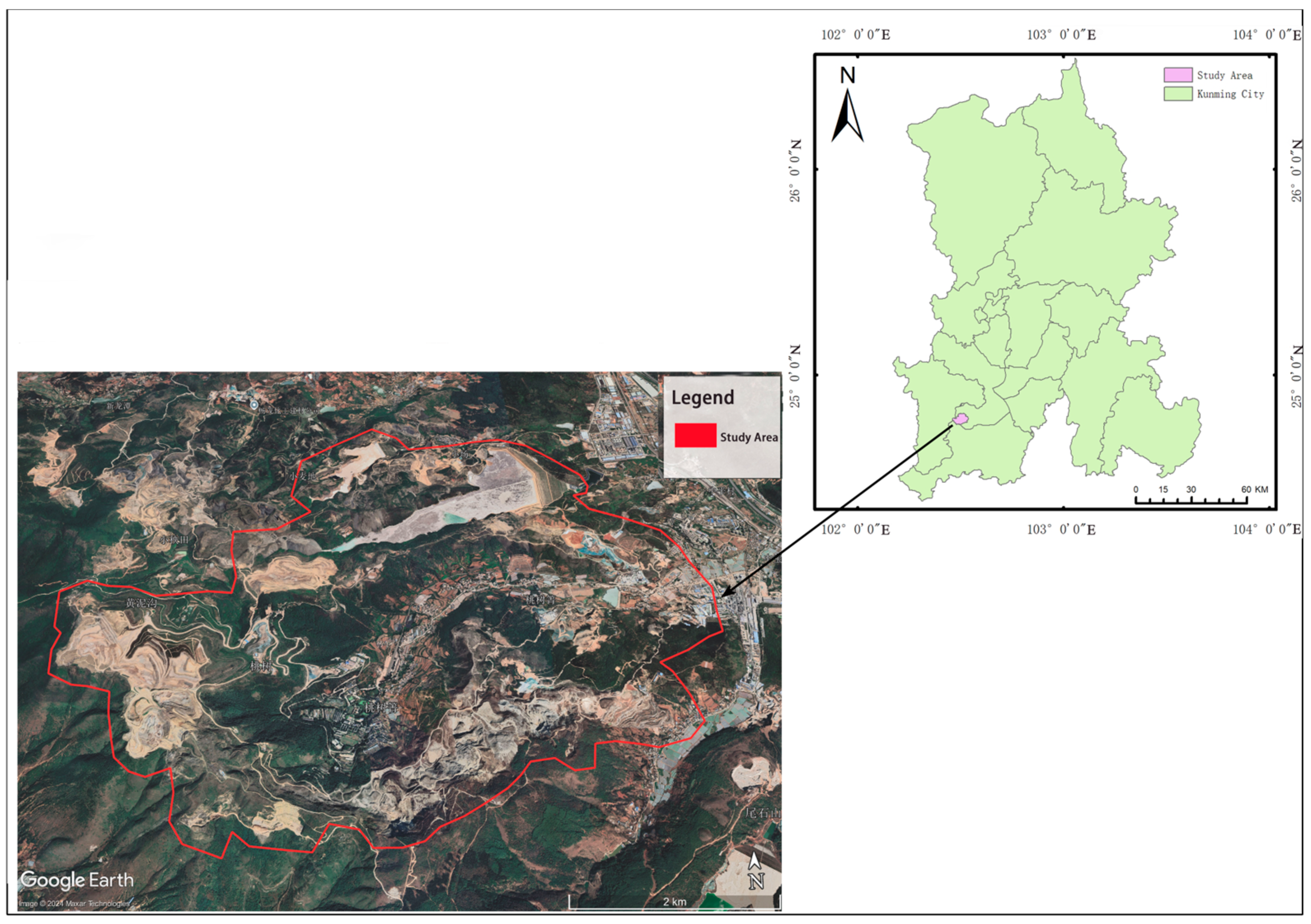
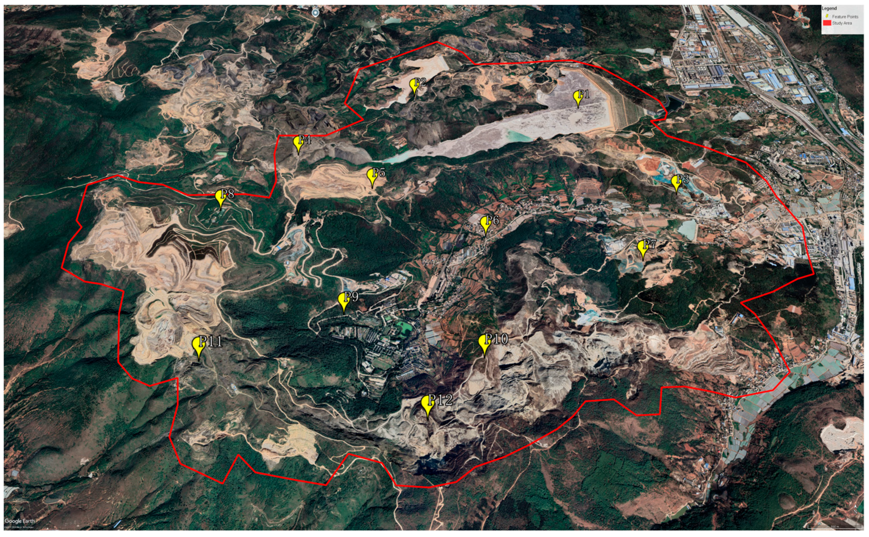
2.1. Study Area Description

Yunnan Province hosts China’s largest phosphate reserves, with Kunming, its capital city, serving as a primary production hub. The study area focuses on the HaiKou Phosphate Mine in Haikou Township, Xishan District, Kunming. The mining area is situated at the southwestern outlet of Lake Dianchi, bordering Jinning and Anning districts to the south and the Xishan Longmen scenic area to the north. Characterized by a northern subtropical plateau monsoon climate, the region exhibits a mean annual temperature of 13.2 °C and annual precipitation of approximately 1000 mm, predominantly occurring from May to September.
Topographically, the mining area features a narrow eastern section and expansive central-western zones, with undulating mountainous terrain typical of plateau landscapes. Vegetation predominantly consists of mid-subtropical mixed coniferous and broadleaf forests, with Pinus armandii (Hua Shan pine) as a representative species. These geomorphological and ecological conditions provide both opportunities and challenges for surface deformation monitoring.
The geographical location of the study area is illustrated in Figure 1.

2.2. Data Sources

This study utilized 82 scenes of C-band ascending Sentinel-1A Synthetic Aperture Radar (SAR) images from the European Space Agency (ESA) Copernicus Programme, spanning January 2018 to May 2023. The data were acquired in Interferometric Wide (IW) swath mode with a 24-day temporal resolution, stored as Single Look Complex (SLC) products in VV polarization, and characterized by a spatial resolution of 5 m × 20 m (range × azimuth). These data provided the foundational input for baseline optimization and surface deformation inversion.
Supplementary datasets included the following:
  • Landsat-8 optical imagery (30 m spatial resolution);
  • Precise orbit determination (POD) ephemeris data from the Copernicus Sentinel missions;
  • ALOS World 3D-30m digital elevation model (DEM);
  • Generic Atmospheric Correction Online Service (GACOS) atmospheric delay products;
  • The data sources and applications are summarized in Table 1.

3. Method

The overall technical workflow of this study is illustrated in Figure 2.

3.1. Interferometric Pair Stacking with Sentinel-1A Data and GACOS Atmospheric Correction

Constructing an InSAR baseline network requires maximizing interferometric pair connections to enhance optimization flexibility. However, increasing temporal intervals exacerbate temporal and spatial decorrelation, rendering many low-coherence pairs unusable [17,18]. To balance data redundancy with the usability of interferograms, a spatial baseline threshold of 2% and a temporal baseline limit of 180 days were set, while requiring each scene to retain at least 20 interferometric connections [19,20]. Ultimately, 495 high-quality interferometric pairs were selected, establishing a robust foundation for subsequent baseline optimization and deformation analysis [21]. The baseline connectivity is visualized in Figure 3.
In interferogram stacking processing, the GACOS atmospheric model is applied for atmospheric phase correction. GACOS (Generic Atmospheric Correction Online Service), developed by Li et al., employs the iterative tropospheric decomposition (ITD) model to separate stratified and turbulent components from tropospheric delay, generating 90-m resolution zenith troposphere delay (ZTD) correction images [22,23].
The GACOS products corresponding to each SAR image were downloaded separately, and atmospheric delay phase correction was applied to the generated interferometric pairs during interferogram stacking, aiming to mitigate the impact of atmospheric effects on InSAR monitoring results.

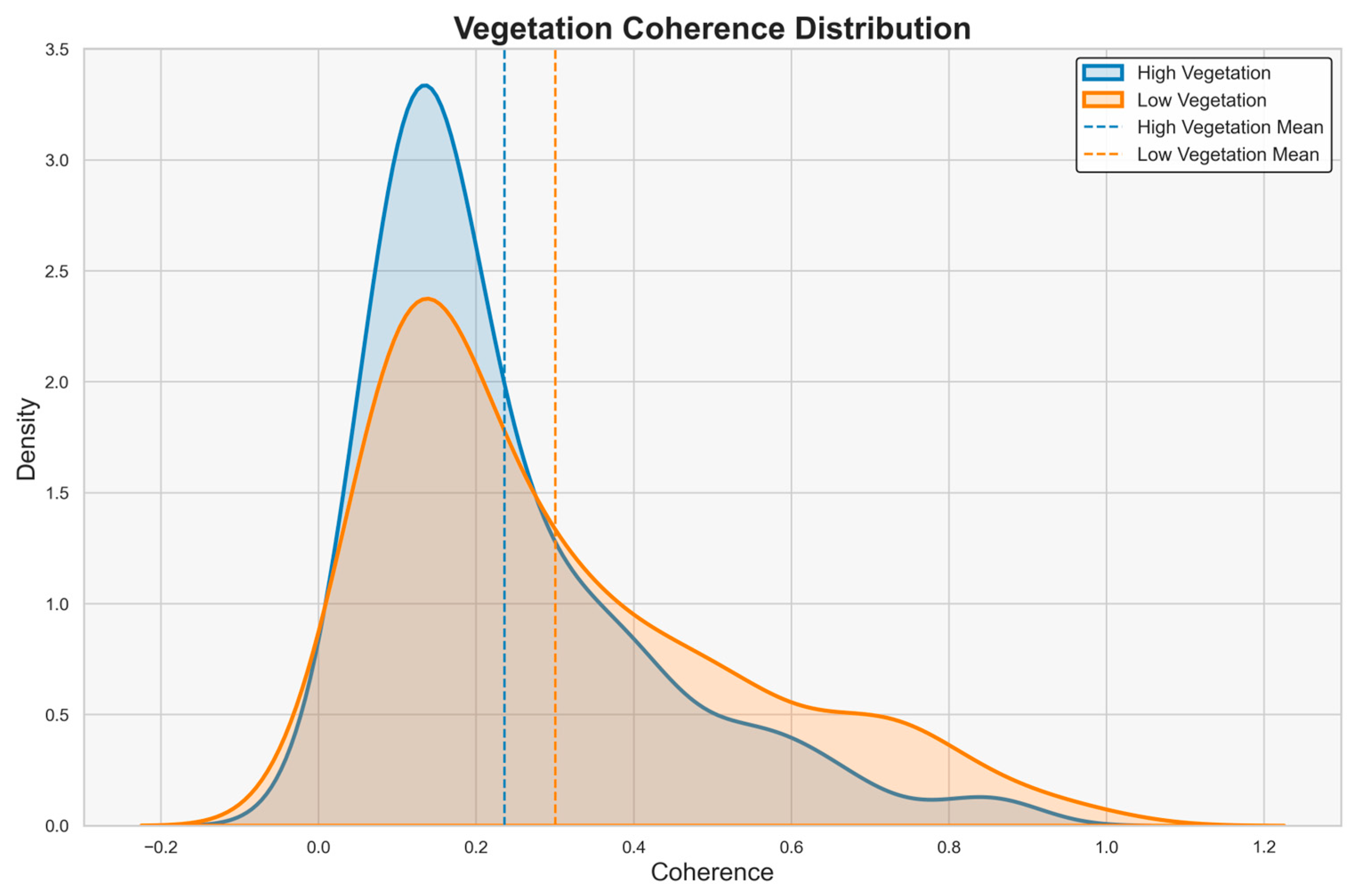
3.2. Spatiotemporal Baselines, Coherence, and NDVI Difference Calculations

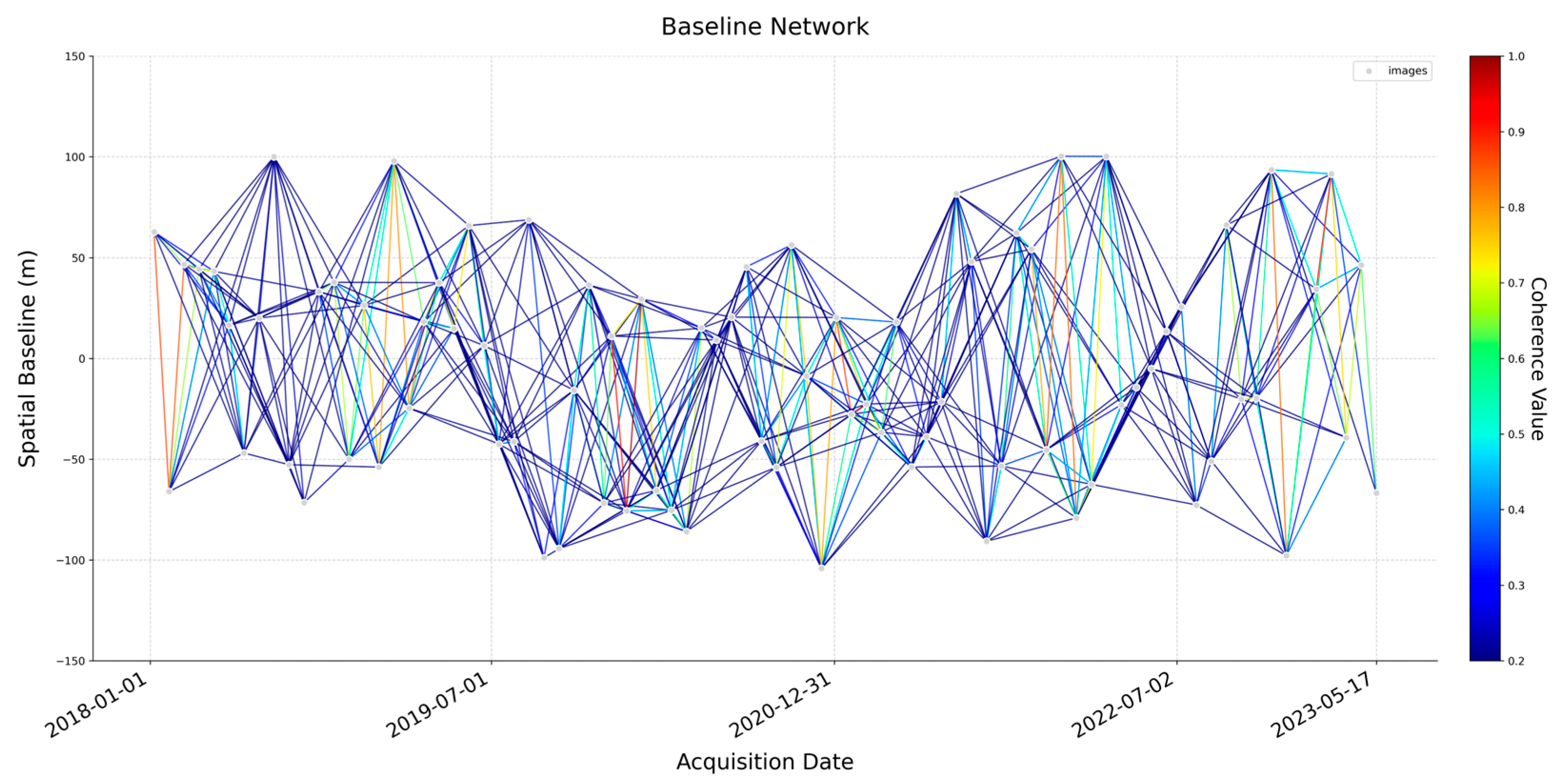
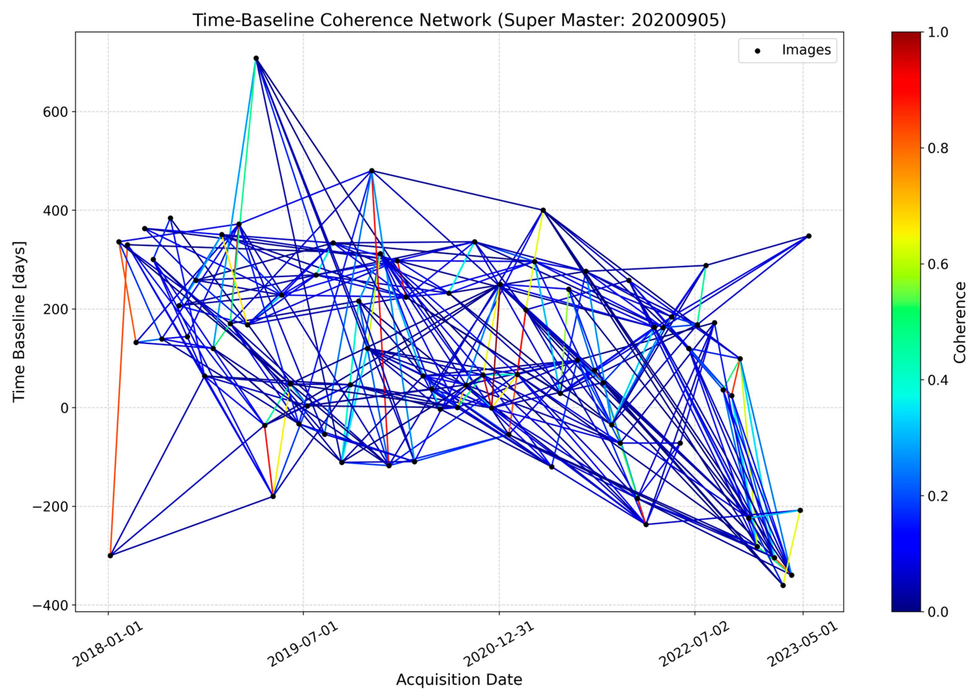
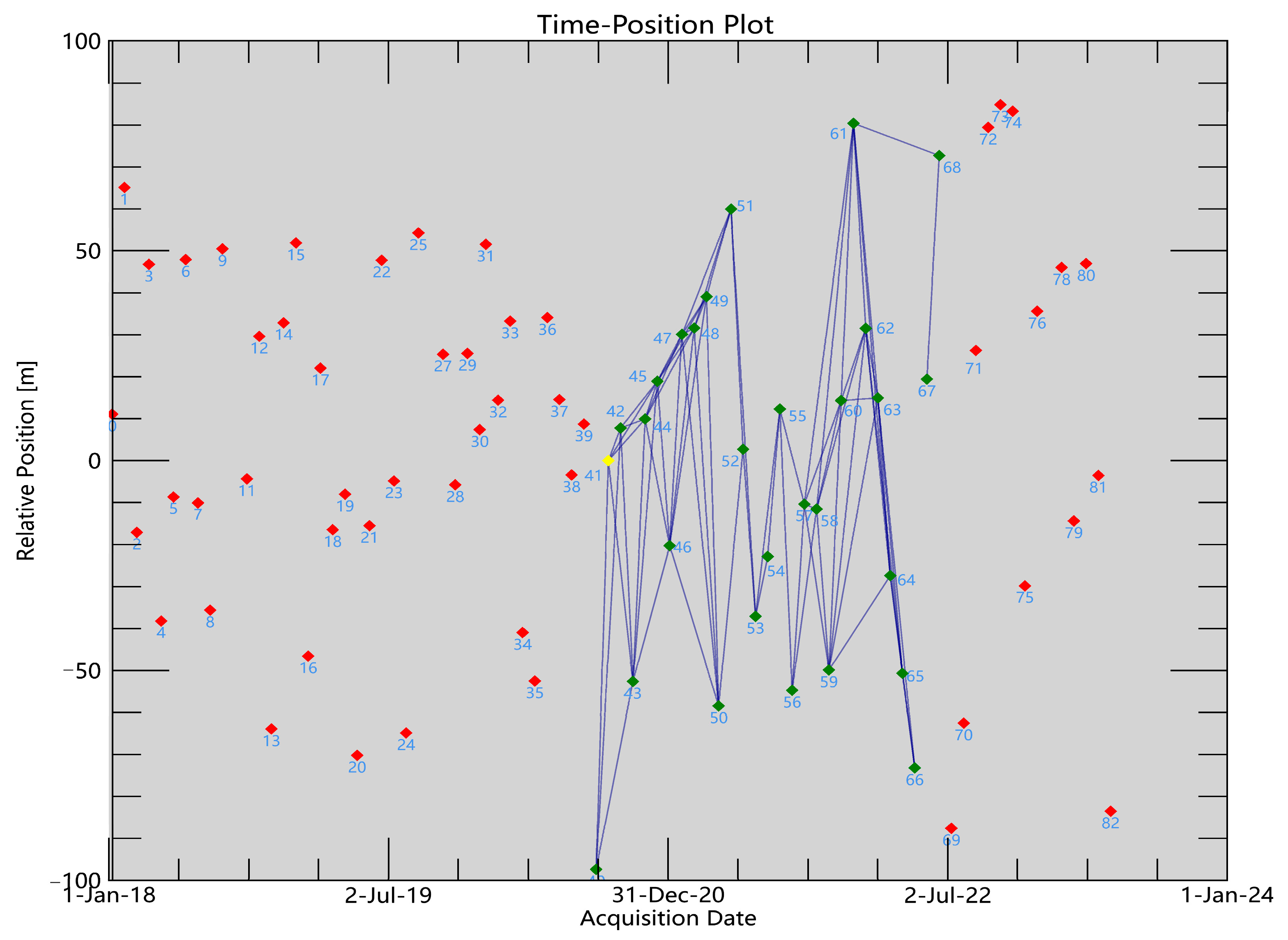
3.2.1. Spatiotemporal Baselines and Coherence Calculation

In interferometric synthetic aperture radar (InSAR), spatial baseline, temporal baseline, and coherence are the core parameters affecting interferogram quality. By integrating spatial baseline, temporal baseline, and coherence, it is possible to optimize the selection of interferometric pairs from multiple dimensions, including geometry, time, and signal stability, thereby improving the accuracy and reliability of deformation monitoring.
In the SBAS-InSAR processing workflow, spatial and temporal baseline data are typically derived from the geometric information of interferometric pairs and are included in the connection graph report. The spatial and temporal baseline information of each interferometric pair can be extracted from the connection graph report, providing the geometric differences between image pairs.
Meanwhile, the coherence coefficient map reflects the coherence between different image pairs, essentially measuring the similarity between two images, typically calculated based on phase differences. Specifically, each pair of images is first precisely registered, and then the phase difference is calculated pixel by pixel, followed by determining the coherence value based on the phase difference. In Python 3.8, this process is efficiently achieved through pixel-wise operations. The commonly used coherence measurement method is the standard coherence coefficient formula:
γ = i = 1 N S 1 ( i ) S 2 * ( i ) i = 1 N S 1 ( i ) 2 i = 1 N S 2 ( i ) 2
where S 1 ( i ) and S 2 * ( i ) represent the complex pixel values of the master and slave images, respectively; the asterisk ( * ) denotes the complex conjugate; and N is the total number of pixels within the calculation window. By obtaining the coherence information and spatiotemporal baseline data of each interferometric pair through the above methods, a quantitative basis is provided for subsequent baseline optimization.

3.2.2. NDVI Difference Calculation

The normalized difference vegetation index (NDVI), proposed by Tucker et al. [24], quantifies vegetation coverage using near-infrared (NIR) and red band reflectance.
N D V I = N I R R E D N I R + R E D
Healthy vegetation exhibits strong NIR reflectance and red light absorption, resulting in high NDVI values, whereas non-vegetated or degraded areas show lower or negative values. To investigate the vegetation dynamics’ impact on deformation, the NDVI difference (ΔNDVI) between master and slave images was calculated as follows:
Δ N D V I = N D V I m a s t e r N D V I s l a v e
Specifically, Landsat-8 optical remote sensing images were first used to obtain the closest observation dates of the master and secondary images for each interferometric pair via the Google Earth Engine (GEE) platform. Then, for each master-secondary image pair, NDVI raster data were calculated for the corresponding areas, and the overall mean NDVI difference was derived from pixel-wise subtraction to reflect the degree of vegetation cover change. Deformation-prone areas typically exhibit decreased ΔNDVI, reflecting vegetation degradation or reduced coverage. ΔNDVI was incorporated as a critical screening criterion to mitigate vegetation-induced decorrelation during interferometric pair selection.

3.3. PCA-Based Baseline Optimization

Principal component analysis (PCA), proposed by Hotelling [25], is a classical method for data dimensionality reduction and feature extraction. PCA projects high-dimensional data onto a set of mutually orthogonal new variables (principal components) through a linear transformation and ranks these components based on the amount of variance they explain. The first few principal components can capture the primary information in the data, simplifying its structure while retaining key features [26].
The significance of PCA lies not only in dimensionality reduction but also in its ability to optimize weight allocation. As noted by Jolliffe [27], PCA provides a clear framework for transforming the intrinsic relationships between complex variables into principal components that are easier to analyze. This characteristic is particularly useful in surface deformation monitoring, where it effectively reduces errors caused by fluctuations in interferogram quality, making it especially suitable for complex monitoring environments [28].
In this study, PCA is used to optimize the selection of interferometric pairs, addressing the complex associations among multiple variables, including temporal baseline, spatial baseline, coherence, and ΔNDVI [27].

3.3.1. Data Preprocessing and PCA Calculation

1.
Data Preparation and Standardization
In this study, PCA is employed to comprehensively evaluate the following four key factors for each interferometric pair. The NDVI difference is obtained by calculating the pixel-wise difference between the NDVI rasters of the master and slave images over the corresponding region, followed by extracting the overall mean value as a statistical indicator of vegetation change. This results in a single numerical value and does not involve direct fusion at the pixel level. The other factors—spatial baseline, temporal baseline, and coherence—are statistical parameters at the regional scale, all sharing a consistent spatial reference framework. Since all factors are extracted and analyzed at the regional level, the issue of inconsistent spatial resolution among multi-source data is effectively avoided, ensuring the rationality of feature integration and the comparability of results.
  • Temporal Baseline (D): The time difference (days) between the master and slave images;
  • Spatial Baseline (S): The geometric distance (meters) between the master and slave images;
  • NDVI Difference (ΔNDVI): The difference in NDVI between the master and slave images, representing vegetation change;
  • Coherence (C): The average coherence of each interferometric pair, indicating image quality.
To eliminate the dimensional differences among these variables, all variables are first standardized using the Z-score method:
X i , j s t d = X i , j μ j σ j
where: X i , j is the element of the original data matrix X in the i-th row and j-th column. μ j is the mean of the j-th column (the j-th variable). σ j is the standard deviation of the j-th column. X i , j s t d is the standardized value of the element in the standardized data matrix.
2.
Calculation of Covariance Matrix
The standardized data matrix X is used to calculate the covariance matrix C, as defined by:
C = 1 n 1 X T X
where C is a 4 × 4 times 4 × 4 square matrix. Each element C i j represents the covariance between the i-th and j-th variables: diagonal elements C i i indicate the variance of each variable; off-diagonal elements C i j indicate the covariance between two variables.
The covariance matrix reveals the linear relationships between variables and serves as the foundation for feature extraction in PCA.
3.
Eigenvalue and Eigenvector Decomposition
Principal components are extracted from the covariance matrix C through eigenvalue decomposition, which yields the eigenvalues and eigenvectors of the matrix. The decomposition is expressed as follows:
C V i = λ i V i
where: V i is the eigenvector of the i-th principal component. λ i is the corresponding eigenvalue, representing the proportion of variance explained by this component.
4.
Calculation of Explained Variance Ratio
The eigenvalues obtained from the decomposition are further used to calculate the explained variance ratio for each principal component. The formula is defined as follows:
E x p l a i n e d   V a r i a n c e   R a t i o = λ i j = 1 n λ j
where λ i is the eigenvalue of the i-th principal component. j = 1 n λ j represents the total number of components.
The principal components are then sorted in descending order based on the explained variance ratio, ensuring that the first few components capture the majority of data variance. Finally, the calculated principal components and their corresponding explained variance ratios are shown in Table 2.

3.3.2. Principal Component Analysis and Weight Calculation

The PCA results demonstrate significant differences among the principal components in explaining data variance. Principal component 1 (PC1, 51.03%) is primarily governed by coherence (+0.6279) and temporal baseline (−0.6295), indicating that the quality of interferometric image pairs is influenced by a combined effect of coherence and temporal interval. Principal component 2 (PC2, 24.97%) is determined by spatial baseline (+0.9989), reflecting its substantial contribution to data variance as an independent variable. Although spatial baseline may theoretically cause baseline decorrelation, its positive weight does not directly indicate a positive or negative impact on interferometric quality. This result may be attributed to the distribution characteristics of spatial baselines and the interactions with other factors in the dataset. Principal component 3 (PC3, 18.17%) is primarily controlled by NDVI difference (+0.8897), revealing the importance of vegetation dynamics within the data. Principal component 4 (PC4, 5.83%) is composed of temporal baseline (+0.7091) and coherence (+0.7046), explaining a smaller proportion of the variance, potentially representing noise components in the data.
Based on the weights of each principal component and their explained variance ratios, the final weight coefficients can be calculated using the following method:
W i = j = 1 m V i j × E V j
where W i is the final weight of the i-th variable, V i j is the weight of the i-th variable in the j-th principal component, and E V j is the explained variance ratio of the j-th principal component.
Based on the results of the principal component analysis, the final weight coefficients are obtained as shown in Table 3.
A comprehensive weighting formula for interferometric pairs was derived as follows:
ω ( u , ν ) = α t ( μ , ν ) + β d ( μ , ν ) + γ Δ N D V I ( μ , ν ) + δ ρ ( μ , ν )
In the equation, ω ( u , ν ) represents the comprehensive weight of interferometric pair ( u , ν ) , where t ( μ , ν ) , d ( μ , ν ) , Δ N D V I ( μ , ν ) , and ρ ( μ , ν ) represent the temporal baseline, spatial baseline, NDVI difference, and coherence of each interferometric pair, respectively. The coefficients α , β , γ , and δ are PCA-derived weight coefficients. The weights determined by PCA only represent the relative contribution of each factor to the principal components (data variance) rather than directly measuring signal quality. The positive weight of the spatial baseline indicates that it carries significant characteristic information within the principal component. Our weighting formula uses the weights determined by PCA to measure the richness of characteristic information in the image pairs, rather than solely focusing on signal fidelity. A higher comprehensive weight indicates that the image pair contains richer “characteristic information” across various factors. Image pairs with richer “characteristic information” exhibit higher quality in InSAR monitoring, especially in complex surface areas.
Pairs were ranked based on their comprehensive weights ω ( u , ν ) , and the lowest 30% of quality were excluded. This screening process resulted in 347 optimized interferometric pairs. The refined baseline network is illustrated in Figure 4.

3.4. SBAS-InSAR Surface Deformation Monitoring Results

The optimized interferometric pairs were subsequently processed using Sarscape 5.6 software to derive surface deformation via the small baseline subset interferometric synthetic aperture radar (SBAS-InSAR) technique. SBAS-InSAR, a time-series InSAR method pioneered by Berardino et al. [29] and Lanari et al. [30] enables high-precision deformation monitoring at centimeter to millimeter-level resolution through temporal phase analysis. This method is particularly suited for large-scale, long-term deformation studies, serving as a critical tool for investigating geological hazards, urban subsidence, and mining-induced deformation.
SBAS-InSAR utilizes multi-temporal SAR images (total N + 1 scenes) from the same orbit to generate interferometric pairs. For the i-th interferogram formed from SAR images acquired at epochs T A and T B , the interferometric phase can be expressed as follows [29]:
Φ ( x , y ) = 4 π λ δ R ( x , y ) + Φ a t m o s ( x , y ) + Φ n o i s e ( x , y )
where λ is the wavelength of the SAR signal, δ R ( x , y ) represents line-of-sight deformation-induced range change, Φ a t m o s ( x , y ) denotes phase contributions from atmospheric delay and sensor errors, and Φ n o i s e ( x , y ) corresponds to phase noise from temporal decorrelation and random effects.
By constructing a time-series interferogram network, SBAS-InSAR extracts deformation signals while mitigating atmospheric and noise artifacts using least-squares inversion and singular value decomposition (SVD) [30]. This approach effectively isolates deformation from non-deformation phase components, making it robust for long-term surface displacement monitoring.

3.5. Comparative Experiment Design

To verify the accuracy of the PCA-optimized SBAS-InSAR deformation results, four comparative experiments were implemented:
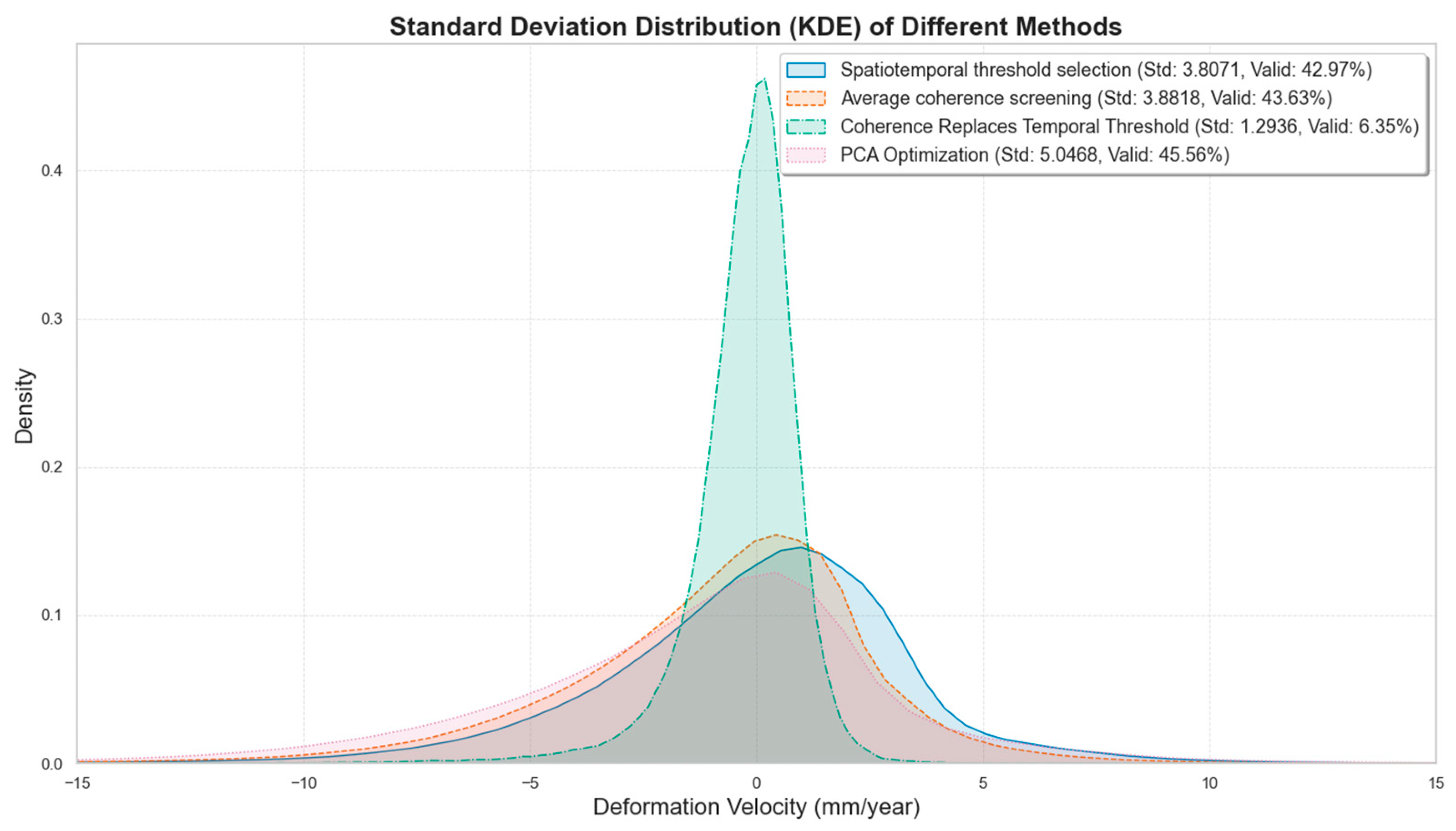
  • Spatiotemporal threshold selection method: All interferometric pairs generated under temporal (180 days) and spatial baseline (2%) thresholds without further screening, followed by SBAS-InSAR processing (Method 1);
  • Average coherence-based screening: Based on the spatiotemporal threshold selection method, all image pairs are ranked in descending order of their average coherence. A 30% threshold (consistent with the PCA method) is set, and the image pairs with lower coherence are removed, followed by SBAS-InSAR processing (Method 2);
  • Coherence-replaced temporal thresholding: Keeping other parameters unchanged from the non-optimized settings, coherence is used instead of the time threshold. By calculating the average coherence of all image pairs and sorting them in descending order, the top 347 pairs (consistent with the number of pairs after PCA optimization) are selected, followed by SBAS-InSAR processing (Method 3);
  • Vegetation-adjusted optimization: Based on the spatiotemporal threshold selection method, the study area is divided into high and low vegetation coverage zones using the fractional vegetation coverage (FVC). Within each zone, image pairs are filtered based on the average coherence of that zone, retaining only those with coherence higher than the average to obtain the final set of pairs, followed by SBAS-InSAR processing (Method 4).
The comparative analysis demonstrated that the PCA-weighted method significantly improved deformation monitoring accuracy by integrating multi-dimensional factors (temporal/spatial baselines, coherence, and ΔNDVI). It effectively reduced the impact of low-coherence pairs, enhanced baseline network robustness, and provided reliable inversion results in complex mining environments.

4. Result

4.1. RMSE Results

The accuracy of SBAS-InSAR inversion using different methods is evaluated by RMSE-RAD (root mean square error of angular deviation), with the results expressed in radians (rad). This metric quantifies the error in InSAR phase estimation, where a smaller value indicates higher inversion accuracy.
Based on the data in Table 4, it can be seen that the PCA-optimized method demonstrates significant advantages in interferogram pair optimization, with overall performance surpassing that of the spatiotemporal threshold selection method, the average coherence screening method, and the coherence-replaced temporal thresholding method. The PCA method reduces the minimum value to 0.248 rad, while the mean and standard deviation decrease to 1.589 rad and 0.797 rad, respectively, clearly outperforming the other methods. Compared to the others, it more effectively suppresses error fluctuations and improves the stability of the results [31,32].
The spatiotemporal threshold selection method shows overall higher indicator values, with relatively large standard deviation and mean, indicating high error levels and poor stability. Although the average coherence screening method reduces the minimum value to 0.335 and lowers the mean to some extent, the maximum value actually increases, and the standard deviation slightly rises, suggesting that relying on a single indicator is insufficient to effectively control error fluctuations [33,34]. The coherence-replaced temporal thresholding method further lowers the minimum value to 0.287; however, both the mean and standard deviation increase significantly, resulting in greater fluctuations and insufficient stability. Additionally, experiments considering vegetation effects failed to extract long-term time series subsidence information, so no further specific results were obtained.
The PCA method achieved optimal performance by scientifically weighting multi-dimensional factors (temporal/spatial baselines, coherence, and ΔNDVI), thereby balancing their impacts on interferogram accuracy.

4.2. Analysis of Other Indicators

Figure 5 and Figure 6 present a comparison of the four methods in terms of deformation rate distribution (probability density function, PDF), effective pixel ratio, and standard deviation. The spatiotemporal threshold selection method and the average coherence threshold method have effective pixel ratios of 42.97% and 43.63%, with standard deviations of 3.8071 mm/year and 3.8818 mm/year, respectively. The coherence-based time threshold method has the lowest effective pixel ratio (6.35%) and the lowest standard deviation (1.2936 mm/year). The PCA-optimized method has the highest effective pixel ratio (45.56%) and the highest standard deviation (5.0468 mm/year).
In the probability density distribution (Figure 6), the spatiotemporal threshold selection method and the average coherence threshold method show distributions concentrated around zero, indicating that most pixel variations are small. The coherence-based time threshold method has a steeper peak, reflecting the strict coherence selection. The distribution curve of the PCA-optimized method is relatively broader, suggesting its ability to capture a wider range of deformation changes. Figure 5 further illustrates the differences among the four methods in terms of valid pixel ratio and standard deviation. Although the PCA method exhibits a slightly higher standard deviation compared to the others, this does not indicate a decline in inversion performance. The increase in standard deviation is primarily due to the inclusion of more low-coherence pixels in edge regions, which, despite introducing some phase noise, also contain real deformation signals. Benefiting from the synergistic effect of multiple factors, the PCA method does not compromise inversion accuracy while enhancing the sensitivity to surface deformation.
Overall, the PCA-optimized method not only maintains a higher effective pixel ratio but also enhances sensitivity to surface deformation changes, indicating its advantage in deformation monitoring in complex terrain areas.
The spatial autocorrelation indicator (Moran’s I) is used to assess the spatial continuity and structural rationality of deformation velocity maps (Table 5). Higher Moran’s I values indicate smoother deformation fields with significant spatial clustering, which aligns with the continuous characteristics of natural processes such as surface subsidence, while also reflecting lower noise levels. By calculating the Moran’s I values for each method, we found that the PCA optimization method not only maintains a high level of spatial autocorrelation but also closely matches the values of traditional methods. This suggests that the deformation velocity data extracted by this method exhibit reasonable and continuous spatial distribution, effectively mitigating the impact of random noise.
In addition, the spatial correlation coefficients between different methods (including Pearson and Spearman coefficients) further validate the consistency of spatial distribution in deformation velocity maps (Table 6). The PCA optimization method demonstrates high spatial correlation with other methods, particularly with the spatiotemporal threshold selection and average coherence screening methods, indicating that it preserves spatial structural characteristics while effectively inheriting the valid information from traditional methods. This suggests that the PCA optimization method improves accuracy without losing the spatial characteristics and physical meaning of the deformation field.
In conclusion, the combined analysis of spatial autocorrelation and spatial correlation coefficients among different methods confirms the advantages of the PCA optimization method in maintaining spatial structure and ensuring result consistency. This supports its capability to achieve higher accuracy and stability in complex surface subsidence monitoring.

4.3. Comparative Experiment Analysis

The study reveals that the HaiKou phosphate mining area is predominantly characterized by low coherence values. As shown in Figure 7, most coherence values are below 0.4, likely due to complex terrain and dense vegetation cover, which induce significant signal scattering and attenuation, resulting in low-coherence features across most interferometric pairs.
In the coherence-replaced temporal thresholding method, 828 interferometric pairs were initially generated (with other parameters unchanged), of which 347 high-coherence pairs were retained after screening (Figure 8). However, the long-term monitoring nature of this approach introduced extended temporal baselines. The network shows pairs with temporal baselines exceeding 200 days, with some surpassing 400 days, leading to pronounced temporal decorrelation—particularly in areas with vegetation dynamics or frequent surface changes. This exacerbates low-coherence phenomena in the study area. Consequently, while the method performs well in regions with high coherence and short temporal baselines, its efficacy remains limited in the HaiKou mining context.
In the HaiKou mining area, the vegetation-adjusted optimization method underperformed in comparative experiments. While this approach partially mitigated vegetation-induced coherence degradation (as shown in Figure 9), the study area’s inherently low-coherence characteristics persisted post-partitioning. Specifically, the method screened 234 pairs in high-vegetation zones and 261 pairs in low-vegetation zones, ultimately retaining only 79 and 101 pairs, respectively.
By applying zone-specific average coherence thresholds, the optimization enhanced the overall mean coherence but excessively excluded low-coherence pairs. This over-filtering led to an overly sparse temporal baseline network (as depicted in Figure 10), ultimately hindering the extraction of long-term deformation time series. Despite its potential efficacy in other regions, the method’s utility remains limited in low-coherence-dominated environments like the HaiKou mining area.

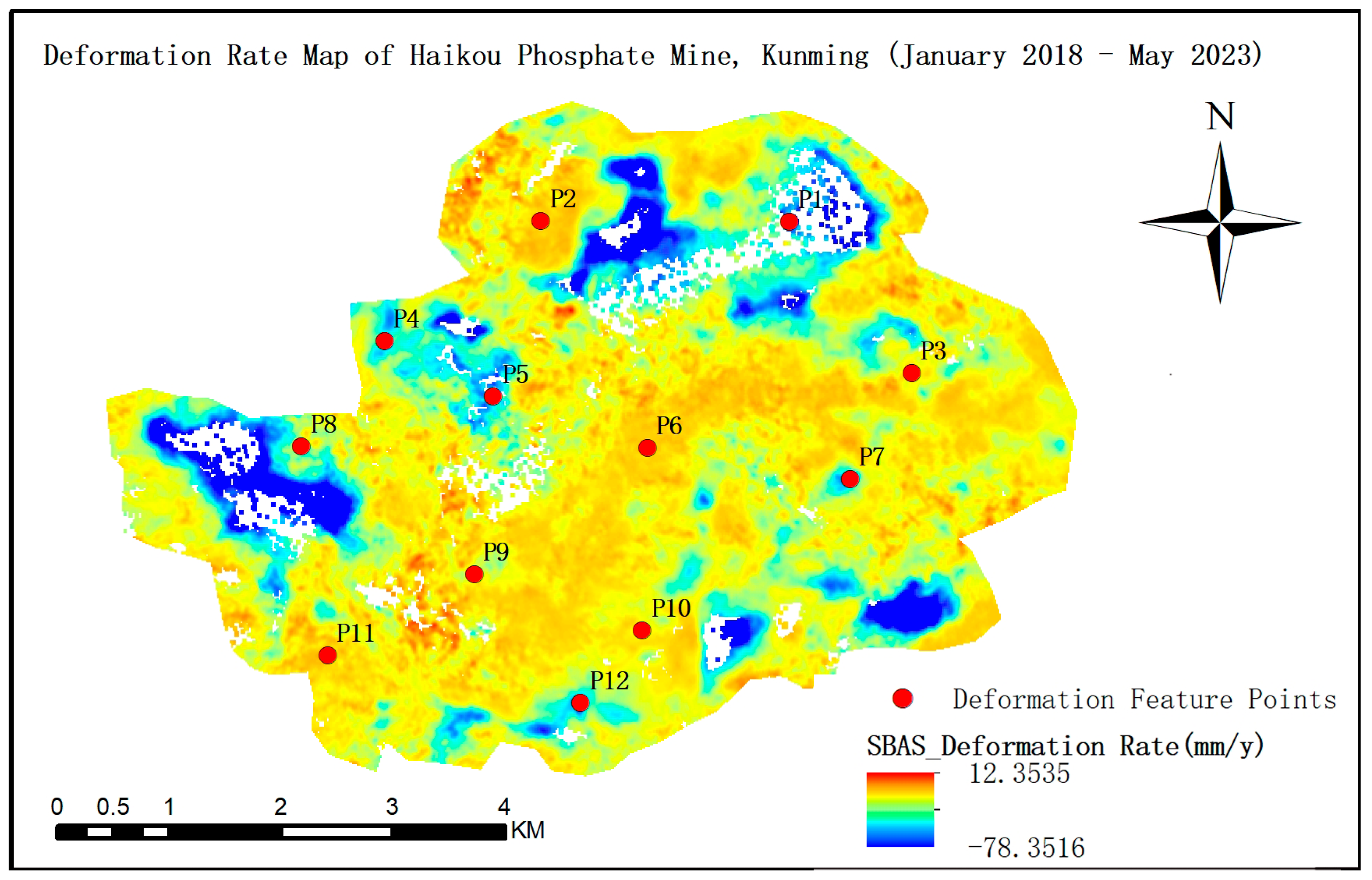
4.4. Analysis of Deformation Results

Based on the PCA-optimized results, Figure 11 and Figure 12 respectively illustrate the cumulative deformation and deformation rate of the Kunming Haikou phosphate mining area from January 2018 to May 2023, clearly revealing the key characteristics of surface deformation in the region. The cumulative deformation map (Figure 11) demonstrates predominant subsidence across the region, with maximum cumulative subsidence exceeding −446 mm in central and southern mining zones. These subsidence features were likely directly linked to prolonged mineral extraction and groundwater depletion [35,36].
The deformation velocity map (Figure 12) further delineates dynamic deformation evolution, showing maximum subsidence rates of −78.351 mm/yr and localized uplift up to +12.353 mm/yr. This indicates sustained subsidence trends coexisting with partial surface rebound phenomena [37]. High-subsidence-rate areas predominantly cluster in zones of intense mining activity, while uplift signals may correlate with ecological restoration efforts or reduced mining intensity [38].
To reveal the spatiotemporal evolution of surface deformation in the study area, 12 representative monitoring points were selected for time series analysis (see Figure 13 and Figure 14). The results show that from January 2018 to May 2023, surface deformation exhibited significant spatial heterogeneity and dynamic variation. Points P2, P6, and P11, located in mountainous areas, generally showed slow uplift, with slight subsidence during the rainy season (April to October), possibly related to rainfall-induced surface disturbances or changes in soil moisture. In contrast, points P1, P4, P5, P7, and P12 within active mining zones showed clear subsidence, reflecting the strong influence of mining activities. Notably, the subsidence rate at point P5 decreased after April 2023, which may be associated with the implementation of ecological restoration measures.
Points P3 and P10, located near the post-mining areas, exhibited minimal deformation, indicating surface stability. Although point P8 is close to the mining zone, its good vegetation coverage led to periodic fluctuations in deformation, suggesting that vegetation played a moderating role and partially offset the impact of mining. Point P9 experienced initial subsidence followed by gradual stabilization and slight rebound, indicating the positive effects of mining cessation and ongoing ecological restoration on surface recovery.

5. Discussion

This study proposes an optimized interferometric pair selection method based on principal component analysis (PCA) weighting, aiming to improve the discriminative accuracy and monitoring stability of interferometric pair selection in InSAR time-series analysis through multi-factor collaborative modeling. Unlike traditional selection strategies that mainly rely on coherence or baseline constraints, the proposed method focuses more on the “information expression capability” of interferometric pairs in a multidimensional feature space. Specifically, a PCA-based weighting system is constructed using NDVI difference, temporal baseline, spatial baseline, and coherence as input factors. The comprehensive weight of each interferometric pair is calculated based on principal component scores. This weight reflects the overall strength of the feature information contained in the pair, rather than the fidelity of a single-dimensional signal. A higher weight indicates that the pair carries more abundant and effective information under the influence of multiple factors, and is therefore more likely to maintain high interferometric quality under complex surface conditions, providing stable support for subsequent deformation monitoring.
From the inversion results, the PCA-optimized method achieves lower RMSE values and a more stable error distribution, outperforming other methods overall. It is worth noting that although the standard deviation of deformation rates is relatively large, this does not indicate a lack of model robustness. Rather, it reflects the higher sensitivity of the multi-factor collaborative weighting mechanism to dynamic surface changes. While ensuring overall inversion accuracy, the method is capable of more sensitively identifying subtle deformation regions, thereby significantly enhancing the adaptability and deformation monitoring sensitivity of InSAR time-series analysis under complex surface conditions. In addition, to address the potential spatial resolution inconsistency in multi-source data fusion, the NDVI difference calculation strategy adopted in this study avoids pixel-level direct fusion between datasets of different resolutions, thereby preventing error propagation and ensuring the scale consistency and reliability of multi-factor integrated analysis.
Of course, the proposed method also has certain limitations. On the one hand, the PCA model does not characterize the causal relationships between factors when performing dimensional weighting, leaving room for improvement in the interpretability of feature contributions. On the other hand, remote sensing indicators such as NDVI are still primarily represented by regional averages, making it difficult to capture local heterogeneity. Future research could further introduce local weighting modeling methods based on regional sliding windows or integrate interpretable machine learning algorithms (such as Random Forest and SHAP value analysis) to enhance understanding and refinement of the contribution mechanisms of different factors. In addition, incorporating more ecological and climatic variables (such as soil moisture, precipitation, and land surface temperature) to construct a more universal interferometric pair selection framework will also be one of the key directions for future optimization.

6. Conclusions

This study proposes an interferometric pair selection method based on principal component analysis (PCA) weighting, establishing a multi-factor collaborative weighted evaluation system combined with a threshold-based filtering mechanism, which effectively improves the quality of interferometric pairs used in SBAS-InSAR deformation inversion. In an empirical study conducted in the Kunming Haikou phosphate mining area, characterized by notably low coherence, the selected interferometric pairs demonstrated significant advantages in deformation inversion accuracy and error control, thereby enhancing the stability and reliability of time-series monitoring results. The inversion outcomes revealed the surface deformation patterns of the mining area from 2018 to 2023, with subsidence zones closely associated with mining activities and ecological restoration efforts.
However, the proposed method still has certain limitations. For instance, its weighting strategy relies on linear combinations of principal components, which may be constrained when dealing with high-dimensional features or strongly nonlinear inter-factor relationships. Future research could consider incorporating nonlinear dimensionality reduction techniques (such as t-SNE, autoencoders) or ensemble learning strategies to improve feature integration capabilities and the adaptive performance of pair selection.
Despite these limitations, this study confirms the applicability of the PCA-based optimization method in InSAR time-series analysis, demonstrating high monitoring accuracy and sensitivity under complex surface conditions—particularly in low-coherence areas. The PCA-based interferometric pair optimization strategy effectively adapts to the complex geological conditions of mining regions and significantly enhances surface deformation monitoring capabilities, offering reliable technical support for ecological restoration assessments. It holds both theoretical significance and practical value, and provides a novel perspective for addressing interferometric pair selection and baseline optimization in InSAR processing.

Author Contributions

The conceptual framework was established by W.X. and J.Z., with research design developed by W.X. and H.M. Experimental execution involved data collection and processing by W.X., X.O. and B.L., while core data analysis was conducted by W.X. The manuscript was drafted by W.X., under academic supervision from J.Z. and J.W., who ensured methodological rigor. Final revisions were completed by J.Z. All authors have read and agreed to the published version of the manuscript.

Funding

This work was supported by the Yunnan Provincial Science and Technology Project at Southwest United Graduate School [grant numbers 202302A037003].

Data Availability Statement

The Sentinel-1A SAR data used in the study are available through https://search.asf.alaska.edu/#/ (accessed on 1 July 2024); the Landsat 8 imagery and NDVI calculation are available through the Google Earth Engine platform https://earthengine.google.com/ (accessed on 1 September 2024); the Sentinel Precise Orbit Ephemerides (POD) data are available through https://dataspace.copernicus.eu/ (accessed on 1 July 2024); the ALOS World 3D DEM is available through https://www.eorc.jaxa.jp/ALOS/en/aw3d30/data/index.htm (accessed on 1 July 2024); and the GACOS atmospheric correction data are available through http://www.gacos.net/ (accessed on 1 September 2024).

Acknowledgments

We would like to acknowledge the ESA (European Space Agency), JAXA (Japan Aerospace Exploration Agency), and Google Earth for providing open-access data. Additionally, we sincerely appreciate the editors and reviewers for their expertise and constructive suggestions.

Conflicts of Interest

The authors declare no conflicts of interest.

References

  1. Erban, L.E.; Gorelick, S.M.; Zebker, H.A. Groundwater extraction, land subsidence, and sea-level rise in the Mekong Delta, Vietnam. Environ. Res. Lett. 2014, 9, 084010. [Google Scholar] [CrossRef]
  2. Hu, B.; Wang, H.S.; Sun, Y.L.; Hou, J.G.; Liang, J. Long-term land subsidence monitoring of Beijing (China) using the small baseline subset (SBAS) technique. Remote Sens. 2014, 6, 3648–3661. [Google Scholar] [CrossRef]
  3. Hanssen, R.F. Radar Interferometry: Data Interpretation and Error Analysis; Springer: Dordrecht, The Netherlands, 2001. [Google Scholar] [CrossRef]
  4. Smittarello, D.; d’Oreye, N.; Jaspard, M.; Derauw, D.; Samsonov, S. Pair selection optimization for InSAR time series processing. J. Geophys. Res. Solid Earth 2022, 127, e2021JB022825. [Google Scholar] [CrossRef]
  5. Lin, F.; Dong, W.M.; Huang, J.; Zhang, H.Z. Application of deformation monitoring in dam area of Xinjiang Plain Reservoir based on SBAS-InSAR method. Geomat. Sci. Technol. 2024, 12, 150–158. [Google Scholar] [CrossRef]
  6. Pan, G.Y.; Tao, Q.X.; Chen, Y.; Wang, K. Subsidence monitoring and analysis of Jiyang mining area in Shandong Province based on SBAS-InSAR. Chin. J. Geol. Hazard Control. 2020, 31, 100–106. [Google Scholar]
  7. Duan, M.; Xu, B.; Li, Z.W.; Wu, W.H.; Wei, J.C.; Cao, Y.M.; Liu, J.H. Adaptively selecting interferograms for SBAS-InSAR based on graph theory and turbulence atmosphere. IEEE Access 2020, 8, 112898–112909. [Google Scholar] [CrossRef]
  8. Wang, S.; Zhang, G.; Chen, Z.; Cui, H.; Zheng, Y.; Xu, Z.; Li, Q. Surface deformation extraction from small baseline subset synthetic aperture radar interferometry (SBAS-InSAR) using coherence-optimized baseline combinations. GISci. Remote Sens. 2022, 59, 295–309. [Google Scholar] [CrossRef]
  9. Falabella, F.; Serio, C.; Zeni, G.; Pepe, A. On the use of weighted least-squares approaches for differential InSAR analyses: The weighted adaptive variable-lEngth (WAVE) technique. Sensors 2020, 20, 1103. [Google Scholar] [CrossRef]
  10. Guo, J.; Xi, W.; Yang, Z.; Huang, G.; Xiao, B.; Jin, T.; Hong, W.; Gui, F.; Ma, Y. Study on optimization method for InSAR baseline considering changes in vegetation coverage. Sensors 2024, 24, 4783. [Google Scholar] [CrossRef]
  11. Lee, J.C.; Shirzaei, M. Novel algorithms for pair and pixel selection and atmospheric error correction in multitemporal InSAR. Remote Sens. Environ. 2023, 286, 113447. [Google Scholar] [CrossRef]
  12. Chen, Y.; Sun, Q.; Hu, J. Quantitatively estimating of InSAR decorrelation based on Landsat-derived NDVI. Remote Sens. 2021, 13, 2440. [Google Scholar] [CrossRef]
  13. Lemmetyinen, J.; Ruiz, J.J.; Cohen, J.; Haapamaa, J.; Kontu, A.; Pulliainen, J.; Praks, J. Attenuation of radar signal by a boreal forest canopy in winter. IEEE Geosci. Remote Sens. Lett. 2022, 19, 2505905. [Google Scholar] [CrossRef]
  14. HZebker, A.; Villasenor, J. Decorrelation in interferometric radar echoes. IEEE Trans. Geosci. Remote Sens. 1992, 30, 950–959. [Google Scholar] [CrossRef]
  15. Massonnet, D.; Feigl, K.L. Radar interferometry and its application to changes in the Earth’s surface. Rev. Geophys. 1998, 36, 441–500. [Google Scholar] [CrossRef]
  16. Ferretti, A.; Prati, C.; Rocca, F. Permanent scatterers in SAR interferometry. IEEE Trans. Geosci. Remote Sens. 2001, 39, 8–20. [Google Scholar] [CrossRef]
  17. Jolivet, R.; Agram, P.S.; Lin, N.Y.; Simons, M.; Doin, M.P.; Peltzer, G.; Li, Z. Improving InSAR geodesy using global atmospheric models. J. Geophys. Res. Solid Earth 2014, 119, 2324–2341. [Google Scholar] [CrossRef]
  18. De Zan, F.; Guarnieri, A.M. TOPSAR: Terrain observation by progressive scans. IEEE Trans. Geosci. Remote Sens. 2006, 44, 2352–2360. [Google Scholar] [CrossRef]
  19. Morishita, Y.; Hanssen, R.F. Temporal decorrelation in L-, C-, and X-band satellite radar interferometry for pasture on drained peat soils. IEEE Trans. Geosci. Remote Sens. 2014, 53, 1096–1104. [Google Scholar] [CrossRef]
  20. Pepe, A.; Lanari, R. On the extension of the minimum cost flow algorithm for phase unwrapping of multitemporal differential SAR interferograms. IEEE Trans. Geosci. Remote Sens. 2006, 44, 2374–2383. [Google Scholar] [CrossRef]
  21. Morishita, Y. Nationwide urban ground deformation monitoring in Japan using Sentinel-1 LiCSAR products and LiCSBAS. Prog. Earth Planet. Sci. 2021, 8, 6. [Google Scholar] [CrossRef]
  22. Xiao, R.; Yu, C.; Li, Z.; He, X. Statistical assessment metrics for InSAR atmospheric correction: Applications to generic atmospheric correction online service for InSAR (GACOS) in Eastern China. Int. J. Appl. Earth Obs. Geoinf. 2021, 96, 102289. [Google Scholar] [CrossRef]
  23. Wang, Q.; Yu, W.; Xu, B.; Wei, G. Assessing the use of GACOS products for SBAS-INSAR deformation monitoring: A case in Southern California. Sensors 2019, 19, 3894. [Google Scholar] [CrossRef] [PubMed]
  24. Tucker, C.J. Red and photographic infrared linear combinations for monitoring vegetation. Remote Sens. Environ. 1979, 8, 127–150. [Google Scholar] [CrossRef]
  25. Hotelling, H. Analysis of a complex of statistical variables into principal components. J. Educ. Psychol. 1933, 24, 417–441. [Google Scholar] [CrossRef]
  26. Abdi, H.; Williams, L.J. Principal component analysis. WIREs Comput. Stat. 2010, 2, 433–459. [Google Scholar] [CrossRef]
  27. Jolliffe, I.T.; Cadima, J. Principal component analysis: A review and recent developments. Philos. Trans. R. Soc. A Math. Phys. Eng. Sci. 2016, 374, 20150202. [Google Scholar] [CrossRef]
  28. Ansari, H.; De Zan, F.; Bamler, R. Efficient phase estimation for interferogram stacks. IEEE Trans. Geosci. Remote Sens. 2018, 56, 4109–4125. [Google Scholar] [CrossRef]
  29. Berardino, P.; Fornaro, G.; Lanari, R.; Sansosti, E. A new algorithm for surface deformation monitoring based on small baseline differential SAR interferograms. IEEE Trans. Geosci. Remote Sens. 2002, 40, 2375–2383. [Google Scholar] [CrossRef]
  30. Lanari, R.; Lundgren, P.; Manzo, M.; Casu, F. Satellite radar interferometry time series analysis of surface deformation for Los Angeles, California. Geophys. Res. Lett. 2004, 31, L23613. [Google Scholar] [CrossRef]
  31. Ferretti, A.; Fumagalli, A.; Novali, F.; Prati, C.; Rocca, F.; Rucci, A. A new algorithm for processing interferometric data-stacks: SqueeSAR. IEEE Trans. Geosci. Remote Sens. 2011, 49, 3460–3470. [Google Scholar] [CrossRef]
  32. Perissin, D.; Wang, T. Time-series InSAR applications over urban areas in China. IEEE J. Sel. Top. Appl. Earth Obs. Remote Sens. 2010, 4, 92–100. [Google Scholar] [CrossRef]
  33. Hooper, A.; Zebker, H.; Segall, P.; Kampes, B. A new method for measuring deformation on volcanoes and other natural terrains using InSAR persistent scatterers. Geophys. Res. Lett. 2004, 31, L23611. [Google Scholar] [CrossRef]
  34. Zhao, R.; Li, Z.; Feng, G.; Wang, Q.J.; Hu, J. Monitoring surface deformation over permafrost with an improved SBAS-InSAR algorithm: With emphasis on climatic factors modeling. Remote Sens. Environ. 2016, 184, 276–287. [Google Scholar] [CrossRef]
  35. Ferretti, A.; Prati, C.; Rocca, F. Nonlinear subsidence rate estimation using permanent scatterers in differential SAR interferometry. IEEE Trans. Geosci. Remote Sens. 2000, 38, 2202–2212. [Google Scholar] [CrossRef]
  36. Cigna, F.; Osmanoğlu, B.; Cabral-Cano, E.; Dixon, T.H.; Ávila-Olivera, J.A.; Garduño-Monroy, V.H.; DeMets, C.; Wdowinski, S. Monitoring land subsidence and its induced geological hazard with Synthetic Aperture Radar Interferometry: A case study in Morelia, Mexico. Remote Sens. Environ. 2012, 117, 146–161. [Google Scholar] [CrossRef]
  37. FRaspini; Bianchini, S.; Ciampalini, A.; Del Soldato, M.; Solari, L.; Novali, F.; Del Conte, S.; Rucci, A.; Ferretti, A.; Casagli, N. Continuous, semi-automatic monitoring of ground deformation using Sentinel-1 satellites. Sci. Rep. 2018, 8, 7253. [Google Scholar] [CrossRef]
  38. Li, D.; Deng, K.; Gao, X.; Niu, H. Monitoring and analysis of surface subsidence in mining area based on SBAS-InSAR. Geomat. Inf. Sci. Wuhan Univ. 2018, 43, 1531–1537. [Google Scholar] [CrossRef]
Figure 1. Geographical location of the study area.
Remotesensing 17 02163 g001
Figure 2. Overall technical workflow of the study.
Remotesensing 17 02163 g002
Figure 3. Unoptimized coherence-baseline network of the interferometric pairs.
Remotesensing 17 02163 g003
Figure 4. PCA-optimized coherence baseline network.
Remotesensing 17 02163 g004
Figure 5. Comparison of effective pixel ratio and standard deviation.
Remotesensing 17 02163 g005
Figure 6. Probability density distribution of deformation rate.
Remotesensing 17 02163 g006
Figure 7. Spatial coherence distribution map.
Remotesensing 17 02163 g007
Figure 8. Baseline network optimized by replacing temporal thresholds with coherence-based selection.
Remotesensing 17 02163 g008
Figure 9. Vegetation-partitioned coherence map.
Remotesensing 17 02163 g009
Figure 10. Temporal baseline distribution post-zoning.
Remotesensing 17 02163 g010
Figure 11. Cumulative deformation map.
Remotesensing 17 02163 g011
Figure 12. Deformation velocity map.
Remotesensing 17 02163 g012
Figure 13. Distribution of monitoring points.
Remotesensing 17 02163 g013
Figure 14. Time series of cumulative deformation.
Remotesensing 17 02163 g014
Table 1. Summary of data sources and applications.
DatasetTime SpanResolutionSourceApplication
Sentinel-1A SARMay 2018–May 20235 × 20 m (range × azimuth)ESA Copernicus ProgrammePrimary dataset for SBAS-InSAR baseline optimization and deformation inversion
Landsat-8May 2018–May 202330 mUSGS/NASANDVI difference calculation
Precise Orbit Determination (POD)May 2018–May 2023N/AESA Copernicus SentinelOrbital error correction
ALOS World 3D-30 m DEMMay 2018–May 202330 mJapan Aerospace Exploration Agency (JAXA)Topographic phase removal
GACOS atmospheric productsMay 2018–May 202390 mUniversity of Newcastle, UKAtmospheric delay mitigation
Table 2. Principal component analysis (PCA) results.
Principal ComponentExplained Variance RatioTemporal Baseline (Days)Spatial Baseline (m)ΔNDVICoherence
PC10.5103−0.6295−0.4000−0.45590.6279
PC20.2497−0.04040.9989−0.02180.0073
PC30.1817−0.31500.00430.88970.3304
PC40.05830.70910.0233−0.01070.7046
Table 3. Final weights of influencing factors.
FactorWeight
Temporal Baseline (days)−0.3472
Spatial Baseline (m)0.2311
ΔNDVI−0.0770
Coherence0.4234
Table 4. RMSE comparison results.
MethodMinMaxMeanStd
Spatiotemporal threshold selection method0.5787.6692.0980.842
Average coherence screening0.3358.0801.7950.859
Coherence-replaced temporal thresholding0.2877.8412.3240.932
Vegetation-adjusted methodN/AN/AN/AN/A
PCA-optimized method0.2487.6001.5890.797
Table 5. Moran’s I results.
MethodsMoran’s I
Spatiotemporal threshold selection method3.7510
Average coherence screening3.7289
Coherence Replaces Temporal Threshold3.6110
PCA Optimization3.7221
Table 6. Spatial correlation coefficients between different methods.
Method PairPearsonSpearman
Spatiotemporal threshold selection method vs. Average Coherence Screening0.88110.8232
Spatiotemporal threshold selection method vs. Coherence Replaces Temporal Threshold0.66980.4627
Spatiotemporal threshold selection method vs. PCA Optimization0.80130.7199
Average Coherence Screening vs. Coherence Replaces Temporal Threshold0.64950.4466
Average Coherence Screening vs. PCA Optimization0.81040.7272
Coherence Replaces Temporal Threshold vs. PCA Optimization0.66370.5280
Disclaimer/Publisher’s Note: The statements, opinions and data contained in all publications are solely those of the individual author(s) and contributor(s) and not of MDPI and/or the editor(s). MDPI and/or the editor(s) disclaim responsibility for any injury to people or property resulting from any ideas, methods, instructions or products referred to in the content.

