Bayesian Denoising Algorithm for Low SNR Photon-Counting Lidar Data via Probabilistic Parameter Optimization Based on Signal and Noise Distribution

Abstract

The Ice, Cloud, and land Elevation Satellite-2 has provided unprecedented global surface elevation measurements through photon-counting Lidar (Light detection and ranging), yet its low signal-to-noise ratio (SNR) poses significant challenges for denoising algorithms. Existing methods, relying on fixed parameters, struggle to adapt to dynamic noise distribution in rugged mountain regions where signal and noise change rapidly. This study proposes an adaptive Bayesian denoising algorithm integrating minimum spanning tree (MST) -based slope estimation and probabilistic parameter optimization. First, a simulation framework based on ATL03 data generates point clouds with ground truth labels under varying SNRs, achieving correlation coefficients > 0.9 between simulated and measured distributions. The algorithm then extracts surface profiles via MST and coarse filtering, fits slopes with >0.9 correlation to reference data, and derives the probability distribution function (PDF) of neighborhood photon counts. Bayesian estimation dynamically selects optimal clustering parameters (search radius and threshold), achieving F-scores > 0.9 even at extremely low SNR (1 photon/10 MHz noise). Validation against three benchmark algorithms (OPTICS, quadtree, DRAGANN) on simulated and ATL03 datasets demonstrates superior performance in mountainous terrain, with precision and recall improvements of 10–20% under high noise conditions. This work provides a robust framework for adaptive parameter selection in low-SNR photon-counting Lidar applications.

1. Introduction

On 15 September 2018, NASA launched the Ice, Cloud, and land Elevation Satellite-2 (ICESat-2), a state-of-the-art mission designed to measure and detect changes in ice sheet elevation, land elevation, and global vegetation height [1,2,3,4,5,6,7,8,9]. Equipped with the Advanced Topographic Laser Altimeter System (ATLAS), ICESat-2 generates six laser beams comprising three strong and three weak beams arranged in three pairs. By leveraging the photon-counting system, ICESat-2 operates at a frequency of 10 kHz at 500 km, resulting in a footprint spacing of ~0.7 m on Earth’s surface [10,11]. This advanced capability extends the applications of ICESat-2 to many other fields, including determining shallow water bathymetry [12,13,14], monitoring water level and ocean dynamics [15,16,17], and detecting the structure of cloud and water column profiles [18,19,20,21]. However, a significant challenge arises from the photon-counting detectors’ sensitivity to solar background radiation, where the signal-to-noise ratio (SNR) during the daytime can degrade by a factor of more than 100 compared to the traditional full-waveform Lidar [22,23,24,25,26]. Therefore, distinguishing signal photons from noise photons under strong solar background conditions remains a critical challenge for ICESat-2 data applications.

To address this issue, several photon-counting Lidar denoising algorithms have been proposed, capitalizing on the fact of a typically higher density for signal photons in point clouds. For instance, the ATL03 product employs an adaptive grid method for signal extraction [27]. While computationally efficient for large-scale applications, this algorithm performs poorly under low SNR conditions. Building on this, the Differential, Regressive, and Gaussian Adaptive Nearest Neighbor (DRAGANN) filtering technique was developed to produce ATL08 product [28], yet its denoising efficacy remains limited in rugged mountainous regions with low SNR. Further advancements include the work of Xiao et al. [29] and Ma et al. [30], who derived the probability distribution function (PDF) of the KNN (K-Nearest Neighbors) distance for two-dimensional space points and applied Bayesian estimation to distinguish between signal and noise photons, thereby identifying optimal denoising threshold for different noise rates. However, the derivation process of PDF assumes that photons are uniformly distributed in space and does not take into account the distribution characteristics of signal and noise photons.

In addition, a spatial density-based clustering algorithm (the Density-Based Spatial Clustering of Applications with Noise, DBSCAN) originally developed for image processing was introduced to photon-counting Lidar by Zhang et al. [31,32,33]. After careful refinement, this method has been successfully applied to the MABLE and ICESat-2 datasets [34,35], enabling signal photon extraction, particularly in complex environments with forest vegetation [35,36]. Subsequent studies have further enhanced the algorithm’s capabilities, including rotating the ellipse in all directions to search for neighbors of DBSCAN [37], which improves adaptability to varying surface slopes, using strong beam information to estimate the slope of the weak beam to select the direction parameters [38]. Other recently developed methods include the optical-based signal extraction algorithm (OPTICS) proposed by Zhu et al. [39] and the quadtree method to transform the spatial coordinates of photons into a tree-like structure proposed by Zhang et al. [40]. Despite these advancements, most existing methods rely on empirical selection of search neighborhoods. In rugged mountainous regions with rapidly changing slopes, fixed search neighborhoods fail to meet the denoising requirements, making slope estimation an indispensable step in denoising algorithms.

This study addresses two critical gaps in photon-counting Lidar denoising: (1) the inability of existing methods to adaptively select parameters under rapidly changing slopes and noise levels, and (2) the scarcity of validation datasets with ground truth labels. To bridge these gaps, we propose a MST Bayesian framework that synergizes slope-aware feature extraction with probabilistic parameter optimization. The framework operates in three phases: (1) rough surface profile extraction using MST; (2) slope estimation from extracted feature points; and (3) adaptive parameter optimization using Bayesian estimation from signal and noise distribution. The algorithm is rigorously evaluated on both simulated data (correlation > 0.9 between simulation and ICESat-2 measurements) and real ATLAS datasets, demonstrating robust performance in steep slopes (>40°) and extreme noise environments. This study can provide theoretical guidance for optimal parameter selection.

2. Materials

2.1. Datasets

2.1.1. ATLAS Data

The ICESat-2/ATLAS instrument is equipped with a green laser at 532 nm with a repetition frequency of 10 kHz, producing footprints with a spacing of 0.7 m in the along-track direction. Each emitted laser pulse is separated by diffractive optical elements, resulting in the generation of six beams (consisting of three strong and three weak beams). In the cross-track direction, the separation between the beam pairs is approximately 3.3 km, while the distance between the strong and weak beams is about 90 m [41]. The data products are categorized into different levels to meet the specific application requirements. In this study, we utilize the Level 2 ATL03 product [42] and Level 3A ATL08 product [43]. The ATL03 data product provides the time tag, longitude, latitude, height, and ancillary data for each photon that ICESat-2 downlinks. In addition, the ATL03 algorithm classifies each photon event as either a noise photon event or a signal photon event, and assigns a confidence label to each photon. The ATL08 product, on the other hand, employs the Differential, Regressive, and Gaussian Adaptive Nearest Neighbor (DRAGANN) filtering algorithm to identify and remove noise photons from the ATL03 point cloud data [28], providing estimations of terrain heights, canopy heights, and canopy cover at fine spatial scales in the along-track direction.

In this study, eight tracks of ATL03 and ATL08 data were selected from three regions (as illustrated in Figure 1 and

Table 1. Information of the used ICESat-2/ATL03 data in this study.

Area	Name	Track Number	Track Used	Date
Eastern Utah	Data 1	ATL03_20231018193445_04552106_006_02	gt3L	2023.10.18
	Data 2	ATL03_20220121015652_04551406_005_01	gt2L	2022.01.21
	Data 3	ATL03_20200425081752_04550706_005_01	gt3L	2020.04.25
	Data 4	ATL03_20210821091308_08971206_005_01	gt3R	2021.08.21
	Data 5	ATL03_20220421213643_04551506_005_02	gt3R	2022.04.21
Altun Mountain in Tibet	Data 6	ATL03_20221001003812_01571706_005_01	gt2L	2022.10.01
	Data 7	ATL03_20210926055926_00581302_005_01	gt2L	2021.09.26
Southern Nevada	Data 8	ATL03_20220613192251_12631506_005_01	gt2L	2022.06.13

). D1–D4 are utilized to generate simulation data and validate the simulation data, which in turn validates the effectiveness of the denoising algorithm under different noise scenarios. Specifically, Data 1 was used to verify the correctness of the simulation method. Data 2 served as the reference track for generating simulated data based on airborne point cloud data. To create ICESat-2/ATLAS simulation data, noise photon clouds with varying noise rates were added to Data 3 and Data 4 (which are nighttime data). Data 5–8 consist of daytime point clouds from the ATL03 weak beams. These beams were used to validate the algorithm’s extraction effect in real-life scenarios with low signal-to-noise ratios. In addition, the true classification labels of daytime point clouds were manually marked to evaluate the denoising performance of the proposed algorithm.

2.1.2. Airborne Data

From 10 June to 29 July 2020, the Utah Automated Geographic Reference Center completed the collection of topographic Lidar data for Eastern Utah and the surrounding area. The data collection was primarily conducted using the Leica TerrainMapper airborne Lidar system. A 32-bit GeoTIFF digital surface model (DSM) was constructed from the initial return points in the processed Lidar dataset, with all overlapping points excluded. Each pixel (1 m × 1 m) in the DSM represents an elevation value. The accuracy of airborne Lidar elevation data was assessed by comparing it with the ground control point elevations, which indicates better than 0.20 m (at 95% confidence level) in non-vegetated areas and better than 0.30 m in vegetated areas. The data was downloaded from The National Map (TNM) download application (https://apps.nationalmap.gov, accessed on 5 January 2024).

2.2. Photon Event Simulation Method of a Lidar

For denoising algorithms, the ergodic and abundant test data are crucial to verifying and improving the algorithms. Although ICESat-2/ATLAS has operated in orbit for many years and provides extensive point cloud data, it is difficult to obtain all possible scenarios for fixed areas of interest. Additionally, determining all signal photons from measured photon clouds is challenging, as the manual labeling used in many studies requires significant efforts and carries inherent subjectivity [38,44]. To address these issues, a simulation method is employed to generate datasets with correct classification labels for all photons, which can significantly expand the amount of data available for performance testing of algorithms in different scenarios.

The energy distribution of the laser pulse emitted by a photon-counting Lidar can be represented by a two-dimensional Gaussian function in the cross section, while its temporal distribution can be described by a one-dimensional Gaussian function approximation. The normalized energy distribution of the emitted pulse in the space domain and in the time domain are shown in Equations (1) and (2).

$${\left|a(l,R_h)\right|}^2={\displaystyle \frac{1}{2\pi {(R_h\tan {\theta }_T)}^2}}\exp \left(-l^2/2R_h^2{\tan }^2{\theta }_T\right).$$

(1)

θ_T is the beam divergence angle, R_h is the flight height, and l is the distance to the spot center in the reflected target cross section. If the target can be considered as Lambertian, the time distribution of the expected photon numbers received by the receiving telescope can be approximated as [45,46,47].

$$N_0(t)=N_0{{\displaystyle {\iint }_{\Sigma }\left|a(l,R_h)\right|}}^2\cdot {\left|f[t-{\displaystyle \frac{2R_h}{c}}-{\displaystyle \frac{l^2}{c{R}_h}}+{\displaystyle \frac{2\xi (l)}{c}}]\right|}^2{d}^{2}l.$$

(2)

N₀ is the total number of received signal photons, c is the speed of light, and ξ(l) is the surface roughness within the spot range.

For a photon-counting Lidar, the number of received photons per the unit time interval satisfies the Poisson distribution. Due to the additivity of the Poisson distribution and considering the noise rate f_n, the number of the total received photons N within the range gate, T_gate obeys the Poisson distribution as [48,49].

$$N~Poisson\left(f_n\cdot T_{gate}+N_{gat\mathrm{e}}\right),$$

(3)

where N_gate represents the expected number of received signal photons within the range gate T_gate. The response characteristics of the PMT (photo-multiplier tube) detector are simulated based on the previously established pileup effect [50,51,52,53]. Specifically, when a photon strikes the detector and triggers the generation of a current pulse, subsequently arriving photons within a defined time window will exhibit temporal overlap with the initial pulse. This superposition effect renders the rising-edge detection method ineffective in recording subsequent photon events. In consideration of the aforementioned factors, the flowchart for simulating the point cloud is shown in Figure 2. The simulation process can be summarized as follows [52].

Step (1): Set the necessary parameters for the simulation: noise rate f_n, the expected number of received signal photons N_gate, the quantity of pulses n_pulse, rise time of the output current t_rise, the tail time of the output current t_rise, and the range gate T_gate. Step (2): The simulated echo waveform is generated using Equation (2). Step (3): The numbers of noise photons and signal photons are randomly generated based on Equation (3). Step (4): The simulated waveforms are discretized into successive time bins, and the expected number of received photons within each time bin is calculated. Step (5): The time tags of signal photons are determined according to the probability distribution and assigned to each bin. Then the time tags of the noise are determined randomly according to uniform distribution. Step (6): The output current is obtained by convolving the photon distribution with the current output response function. Finally, the time tag when the rising edge of the output current exceeds the discrimination threshold is taken as the time tag of the recorded photon event based on the output current.

2.3. Test Dataset

To evaluate the performance of the denoising algorithm, a test dataset was constructed using ICESat-2 data with true values manually labeled, along with simulated data. Simulated data were generated using Data 2–4 to validate the theoretical model of the algorithm and the performance of the algorithm. The simulation point clouds with different signal and noise levels are generated based on the reference track of Data 2 based on the local DSM, as shown in Figure 3. Since Data 3 and Data 4 are nighttime data, there are only very few background noise photons (~10 kHz), so the photon events in the data with a confidence level greater than 3 are selected as the reference signal photons (the average signal photon number of Data 2 is about 0.64, and the average signal photon number of Data 3 is about 1.35) and the ATL03-Simulated data are generated by adding the noise photon clouds with different noise ratios based on the noise model (Figure 4). In addition to the simulation data, 10 km segments of weak beam data from four ICEat-2 tracks were used to verify the denoising performance of the algorithm at low SNR conditions. The weak-beam data of the four tracks are shown in Figure 5.

3. Denoising Method

3.1. PDF Model of Signal and Noise Photons

A key challenge in effectively utilizing the clustering algorithm lies in selecting the critical parameters, i.e., the radius of the search neighborhood (Dia, or the semi-major a and semi-minor axes b for elliptical search neighborhoods) and threshold (Minpts). For each point in the point cloud used for classification, the number of points within the search region is counted. If the number of points is greater than the threshold Minpts, the point is marked as a signal photon; otherwise, it is marked as a noise photon. For different searched neighborhoods, photons can be classified into six categories depending on their position. As shown in Figure 6, the six cases are represented by w_ij, where i represents the signal or noise (1 for noise and 2 for signal) and j represents the position of the photon in the point cloud which is divided according to the position of the photon and the size of the search neighborhood.

3.1.1. PDF of Noise Photons

For different searched neighborhoods, noise photons can be classified into two categories depending on their positions, i.e., the noise photons far from the signal (w₁₁) and noise photons close to the signal (w₁₂ and w₁₃). The calculation of the PDF can be calculated as follows.

w₁₁: According to Section 2.2, the number of photon events recorded in multiple time intervals still satisfies the Poisson distribution, and thus the PDF of the number of recorded photons in the elliptical neighborhood can be approximated as follows:

$$p(Num=k|w_{11})={\displaystyle \frac{{\lambda }^k}{k!}}{e}^{-\lambda },\lambda ={\displaystyle \frac{2\pi ab{k}_{laser}{f}_n}{cv}},k=1,2,3\dots$$

(4)

where a is the half-long axis of the ellipse, b is the half-short axis of the ellipse, k_laser is the frequency of the laser, c is the speed of light, v is the velocity of the Lidar, and f_n is the noise rate.

w₁₂: As shown in Figure 7, when the half-length axis of the search neighborhood satisfies $b-l\le P_{W}c/2$ ($P_W$ is six times of the root-mean-square pulse width, l is the distance between the center photon and the signal region boundary), the neighborhood can be divided into a noise region and a signal region (the same treatment is used in other cases). The area of the noise region can be expressed as follows:

$$S_{12}=\pi ab+2la\sqrt{1-{\displaystyle \frac{l^2}{b^2}}}-{\displaystyle {\int }_{-a\sqrt{1-\frac{l^2}{b^2}}}^{a\sqrt{1-\frac{l}{b^2}}}b\sqrt{1-\frac{x^2}{a^2}}}\mathrm{d}x.$$

(5)

The distribution of photons in the signal region is counted using a hierarchical model. For the signal region, since the density of signal photons is much higher than that of noise photons, the effect of dead time cannot be ignored in the calculation. The resolution dh is set to $dh=0.1\cdot c.$ If the dead time of the detector is t_d, according to the dead time model of photon-counting detectors [50,51,52], the expected value N_k of the number of photons responding to a single pulse in the kth layer can be expressed as follows:

$$\begin{array}{l}{N}_{k_{th}}=(n_s(k_{th})+2f_{n}dh/c)\cdot (1-e^{-{\lambda }_{td}}),\\ {\lambda }_{td}={\displaystyle \sum _{i=k_{th}-t_d/0.1}^{k_{th}-1}{N}_i},\\ N_1=(n_s(1)+2f_{n}dh/c)\cdot (1-e^{-f_n{t}_d}),\\ {\displaystyle \sum N_i}=n_{total}-f_n\cdot {\displaystyle \frac{L{k}_{laser}}{v}}\cdot (2H/c-P_W).\end{array}$$

(6)

n_s(kth) is the expected value of the signal photons received in the kth layer, λ_td is the expected value of the number of photons responding in the dead time range before the kth layer, n_total is the total number of photons in the point cloud, L is the distance in the along-track direction, and H is the elevation range of the point cloud. An iterative solution based on Equation (6) yields the expected value of the number of photons responding to a single shot pulse at each layer.

For the hierarchical model of the signal region, the area of layer i can be expressed as follows:

$$\begin{array}{l}{S}_i={\displaystyle {\int }_{-aX[i-1]}^{aX[i-1]}b\sqrt{1-\frac{x^2}{a^2}}}\mathrm{d}x-2[l+(i-1)dh]aX[i-1]-{\displaystyle {\int }_{-aX[i]}^{aX[i]}b\sqrt{1-\frac{x^2}{a^2}}}\mathrm{d}x+2(l+idh)aX[i],\\ X[i]=\sqrt{1-{\displaystyle \frac{{[l+idh]}^2}{b^2}}},X[i-1]=\sqrt{1-{\displaystyle \frac{{[l+(i-1)dh]}^2}{b^2}}}.\end{array}$$

(7)

The number of photon events recorded in layer i satisfies the Poisson distribution and can be represented as follows:

$$\begin{array}{l}{p}_i(Num=k|w_{12})={\displaystyle \frac{{(\lambda )}^k}{k!}}{e}^{-\lambda },\lambda ={\displaystyle \frac{N_i{k}_{laser}{S}_i}{vdh}}\\ \end{array}$$

(8)

Then, based on the additivity of the Poisson distribution, the PDF of the number of photons in this case can be represented as follows:

$$p(Num=k|w_{12})={\displaystyle \frac{{(\lambda )}^k}{k!}}{e}^{-\lambda },\lambda ={\displaystyle \frac{2S_{12}{k}_{laser}{f}_n}{cv}}+{\displaystyle \sum _{i=1}^{(b-l)/dh}\frac{N_i{k}_{laser}{S}_i}{vdh}.}$$

(9)

w₁₃: When the half-length axis of the search neighborhood satisfies $b-l>P_{W}c/2$, the PDF of the number of photons in the signal region can be represented by Equation (8) and the area of the noise region can be expressed by Equation (9).

$$p(Num=k|w_{13})={\displaystyle \frac{{(\lambda )}^k}{k!}}{e}^{-\lambda },\lambda ={\displaystyle \sum _{i=1}^{(P_{w}c/2)/dh}\frac{N_i{k}_{laser}{S}_i}{vdh}}+{\displaystyle \frac{2S_{13}{k}_{laser}{f}_n}{cv}}.$$

(10)

$$\begin{array}{l}{S}_{13}=\pi ab+2la\sqrt{1-{\displaystyle \frac{l^2}{b^2}}}+{\displaystyle {\int }_{-a\sqrt{1-\frac{{(l+P_{w}c/2)}^2}{b^2}}}^{a\sqrt{1-\frac{{(l+P_{w}c/2)}^2}{b^2}}}b\sqrt{1-\frac{x^2}{a^2}}}\mathrm{d}x-{\displaystyle {\int }_{-a\sqrt{1-\frac{l^2}{b^2}}}^{a\sqrt{1-\frac{l}{b^2}}}b\sqrt{1-\frac{x^2}{a^2}}}\mathrm{d}x\\ -2(l+P_{w}c/2)a\sqrt{1-{\displaystyle \frac{{(l+P_{w}c/2)}^2}{b^2}}}.\end{array}$$

(11)

3.1.2. PDF of Signal Photons

w₂₁: When the half-length axis of the search neighborhood satisfies the following:

$$l\ge b$$

At this time, the neighborhood lies completely in the signal interval, and the PDF of the number of responding photons in the elliptical neighborhood at this time can be approximated by Equation (12).

$$p(Num=k|w_{21})={\displaystyle \frac{{\lambda }^k}{k!}}{e}^{-\lambda },\lambda ={\displaystyle \sum _{i=1}^{b/dh}\frac{N_i{k}_{laser}{S}_i}{vdh}}+{\displaystyle \frac{2\pi ab{k}_{laser}{f}_n}{cv}}+{\displaystyle \sum _{i=b/dh+1}^{2b/dh}\frac{N_i{k}_{laser}{S}_i}{vdh}}.$$

(12)

w₂₂: When the half-length axis of the search neighborhood satisfies $l+b\le P_{w}c/2,l<b$. The PDF of the number of photons in the signal region can be expressed by Equation (13).

$$p(Num=k|w_{22})={\displaystyle \frac{{(\lambda )}^k}{k!}}{e}^{-\lambda },\lambda ={\displaystyle \sum _{i=1}^{l/dh}\frac{N_i{k}_{laser}{S}_i}{vdh}}+{\displaystyle \frac{2S_{22}{k}_{laser}{f}_n}{cv}}+{\displaystyle \sum _{i=l/dh+1}^{(l+b)/dh}\frac{N_i{k}_{laser}{S}_i}{vdh}}.$$

(13)

$$S_{22}={\displaystyle {\int }_{-a\sqrt{1-\frac{l^2}{b^2}}}^{a\sqrt{1-\frac{l}{b^2}}}b\sqrt{1-\frac{x^2}{a^2}}}\mathrm{d}x-2la\sqrt{1-{\displaystyle \frac{l^2}{b^2}}}.$$

(14)

w₂₃: The half-length axis of the search neighborhood satisfies $l+b>P_{w}c/2$. The PDF of the number of photons in the signal region can be represented by Equation (15).

$$p(Num=k|w_{23})={\displaystyle \frac{{(\lambda )}^k}{k!}}{e}^{-\lambda },\lambda ={\displaystyle \sum _{i=1}^{(P_{w}c/2)/dh}\frac{N_i{k}_{laser}{S}_i}{vdh}}+{\displaystyle \frac{2S_{23}{k}_{laser}{f}_n}{cv}}.$$

(15)

$$\begin{array}{l}{S}_{23}={\displaystyle {\int }_{-a\sqrt{1-\frac{l^2}{b^2}}}^{a\sqrt{1-\frac{l}{b^2}}}b\sqrt{1-\frac{x^2}{a^2}}}\mathrm{d}x+{\displaystyle {\int }_{-a\sqrt{1-\frac{{(P_{w}c/2-l)}^2}{b^2}}}^{a\sqrt{1-\frac{{(P_{w}c/2-l)}^2}{b^2}}}b\sqrt{1-\frac{x^2}{a^2}}}\mathrm{d}x\\ -2la\sqrt{1-{\displaystyle \frac{l^2}{b^2}}}-2(P_{w}c/2-l)a\sqrt{1-{\displaystyle \frac{{(P_{w}c/2-l)}^2}{b^2}}}.\end{array}$$

(16)

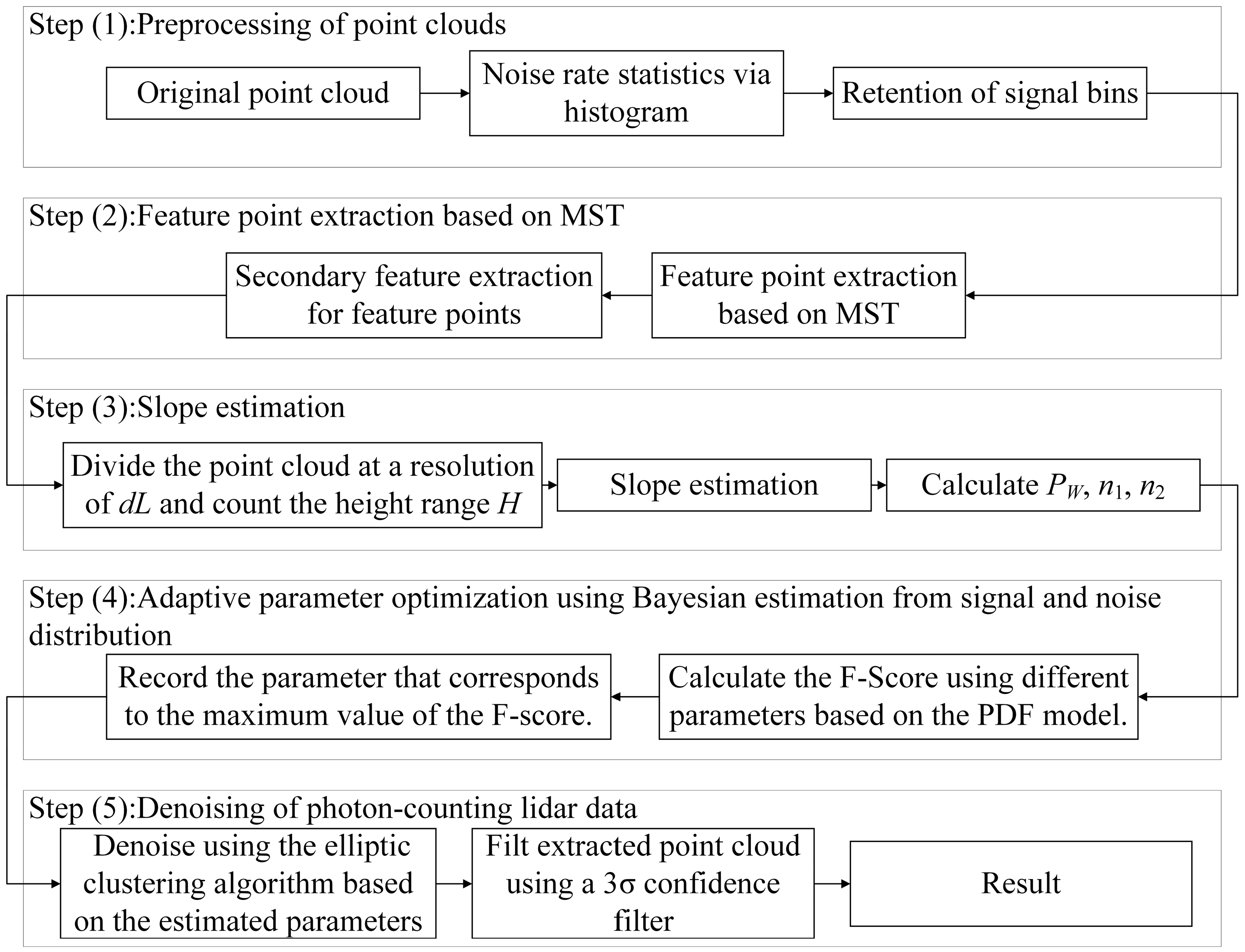
3.2. Denoising Algorithm Based on a MST Bayesian Framework

The denoising algorithm consists of five steps, of which Steps 2–4 are the MST Bayesian framework. The flowchart for the denoising algorithm is shown in Figure 8. The denoising process can be summarized as follows.

Step (1): Preprocessing of point clouds. Referring to the point cloud processing method in ATL03 [27], the original point cloud is segmented in the along-track direction with a step of 60 m. For each segment, a statistical histogram is generated with an elevation resolution of 30 m (i.e., the bin has a width of 60 m and a height of 30 m). The mean and standard deviation of the number of photons in all bins in the histogram are calculated, and the noise rate f_n for the segment is calculated using the portion of the histogram that is less than the mean plus three times of the standard deviations. If there are only noise photons in the data, the distribution of the number of histogram bins with the number of photons in the histogram bin can be calculated as follows:

$$BI{N}_{num}(k)=Nu{m}_{total}\cdot P(Num=k;bin\_w,bin\_h,f_n)$$

(17)

where BIN_num is the number of histogram bins with the number of photons equal to k in a frame range, and Num_total is the number of total histogram bins. Since the theoretical curve is calculated assuming that the point cloud consists only of noisy photons following a Poisson distribution, the statistical values of the bin in which the signal is present will differ from the theoretical curve. Based on this difference, bins that deviate from the theoretical curve are retained as signal bins. Furthermore, the coarsely filtered point cloud undergoes further refinement by assessing the continuity of the point cloud elevation in the along track direction, and the bins that are not retained at the first instance but exhibit continuous elevation are retained.

Step (2): Feature point extraction based on MST. A loop-free connected subgraph G consisting of n nodes and n − 1 edges of a graph G′ is called a spanning tree of the graph G′ (G′ represents a fully connected graph, i.e., all nodes in the graph are connected by edges) [54]. A graph G is a minimal spanning tree of a graph G′ if it is the one with the smallest sum of weights of cost functions among all spanning trees of the graph G. If the graph G is a loop-free connected subgraph generated by point cloud, the cost function between interconnected photons u and v can be defined as the Euclidean distance between them.

$$w(u,v)=\sqrt{{(u_x-v_x)}^2+{(u_y-v_y)}^2},$$

(18)

$$w_G={\displaystyle \sum _{u,v\in G}w(u,v)},$$

(19)

w_G is the total cost of the spanning tree. When w_G reaches the minimum value, the graph G is the minimum spanning tree of the point cloud. There are several existing algorithms to solve the MST problem. In this study, the Prim algorithm is used to generate the MST [54,55], and the MST is generated separately for each 60 m segment of the point cloud. The Prim algorithm is essentially a greedy algorithm that progressively connects the points closest to the generated tree until all points are connected. Considering the density of signal photons is greater than that of noise photons, photons that lie on the longest path (where the path means the number of edges passed from one photon to another in the tree) are extracted as a feature point. If such a path is not unique, the cost function and the smallest one are kept. In addition, to remove the edge effect caused by segmentation, the extracted feature points are resegmented to generate a new MST with a segment length of 1.5 times, followed by secondary feature extraction using the above judgment method.

Step (3): Slope estimation. The slope is estimated by linear fitting using the feature points obtained in Step (2) at a resolution of dL 30 m. The estimated slope values are used to estimate the pulse width P_W [45,46], noise photon count n₁, and signal photon count n₂. n₁ and n₂ can be expressed as Equation (20).

$$\begin{array}{l}{n}_1=f_n\cdot {\displaystyle \frac{dL\cdot k_{laser}}{v}}\cdot (2H/c-P_W),\\ n_2=n_{total}-f_n\cdot {\displaystyle \frac{dL\cdot k_{laser}}{v}}\cdot (2H/c-P_W).\end{array}$$

(20)

Step (4): Adaptive parameter optimization using Bayesian estimation from signal and noise distribution. To optimize the search neighborhood and threshold for the final clustering algorithm, the Bayesian estimation theory is employed to analyze the photon distribution in the point cloud [56]. According to the sub-case of photons in the point cloud, it is assumed that the number of each type of photon in the point cloud is n_ij, where i is taken as 1 or 2 (1 represents the noise photons, 2 represents the signal photons) and j represents the index of a signal or noise photon in the point cloud. When the subscript is only i, n_i represents the total number of noise or signal photons like Equation (20). Then, the prior probability of that type of photon is $p_{ij}=n_{ij}/n_{total}$, where n_total is the total number of photons in the point cloud.

For the photons in the point cloud, when the long axis of the search neighborhood is 2a, the short axis length is 2b, and the number of photons in the neighborhood is k, its posterior probability can be expressed as Equation (21).

$$\begin{array}{l}P(w_1|Num=k)={\displaystyle \frac{{\displaystyle {\sum }_{j}p(Num=k|w_{1j})p_{1j}}}{p(Num=k)}},\\ P(w_2|Num=k)={\displaystyle \frac{{\displaystyle {\sum }_{j}p(Num=k|w_{2j})p_{2j}}}{p(Num=k)}},\\ p(Num=k)={\displaystyle {\sum }_{i,j}p(Num=k|w_{ij})p_{ij}},\end{array}$$

(21)

where $p(Num=k|w_{ij})$ can be obtained from Equations (4)–(16), and w_i indicates a noise photon or a signal photon.

By analyzing the posterior probability distribution, a curve can be generated that relates the photon posterior probability to the number of photons in the neighborhood. This curve is crucial for determining the optimal parameters for the clustering algorithm. To evaluate the performance of the denoising algorithm, three metrics are typically used: the precision (Pre), recall (Rec), and F-score (F) [38,57]. Precision represents the probability of correctly extracted signal photons, while recall denotes the percentage of signal photons in the extracted point cloud. The F-score, which combines precision and recall, is defined as Equation (22).

$$\begin{array}{l}\mathrm{Rec}={\displaystyle \sum _{k\ge Minpts}\frac{P(w_2|Num=k)p(Num=k)}{p(w_2)}},\\ \mathrm{Pre}={\displaystyle \sum _{k\ge Minpts}\frac{P(w_2|Num=k)p(Num=k)}{p(w_2)}}{n}_2/\\ ({\displaystyle \sum _{k\ge Minpts}\frac{P(w_2|Num=k)p(Num=k)}{p(w_2)}}{n}_2\\ +{\displaystyle \sum _{k\ge Minpts}\frac{P(w_1|Num=k)p(Num=k)}{p(w_1)}{n}_1}),\\ \mathrm{F}={\displaystyle \frac{2\cdot \mathrm{Rec}\cdot \mathrm{Pre}}{\mathrm{Rec}+\mathrm{Pre}}},\\ \{a,b,Minpts\}=\mathrm{argmax}\left(\mathrm{F}\right(a,b,Minpts\left)\right).\end{array}$$

(22)

Then, the parameters of the clustering algorithms (a, b, and Minpts) are chosen to distinguish the signal photons when the F-score takes the maximum value.

Step (5): Denoising of photon-counting Lidar data. Based on the parameters estimated by Step (4), the elliptic clustering algorithm is used for denoising, and finally the extracted point cloud is filtered using a three-sigma confidence filter to remove the outliers [38].

4. Model Validation

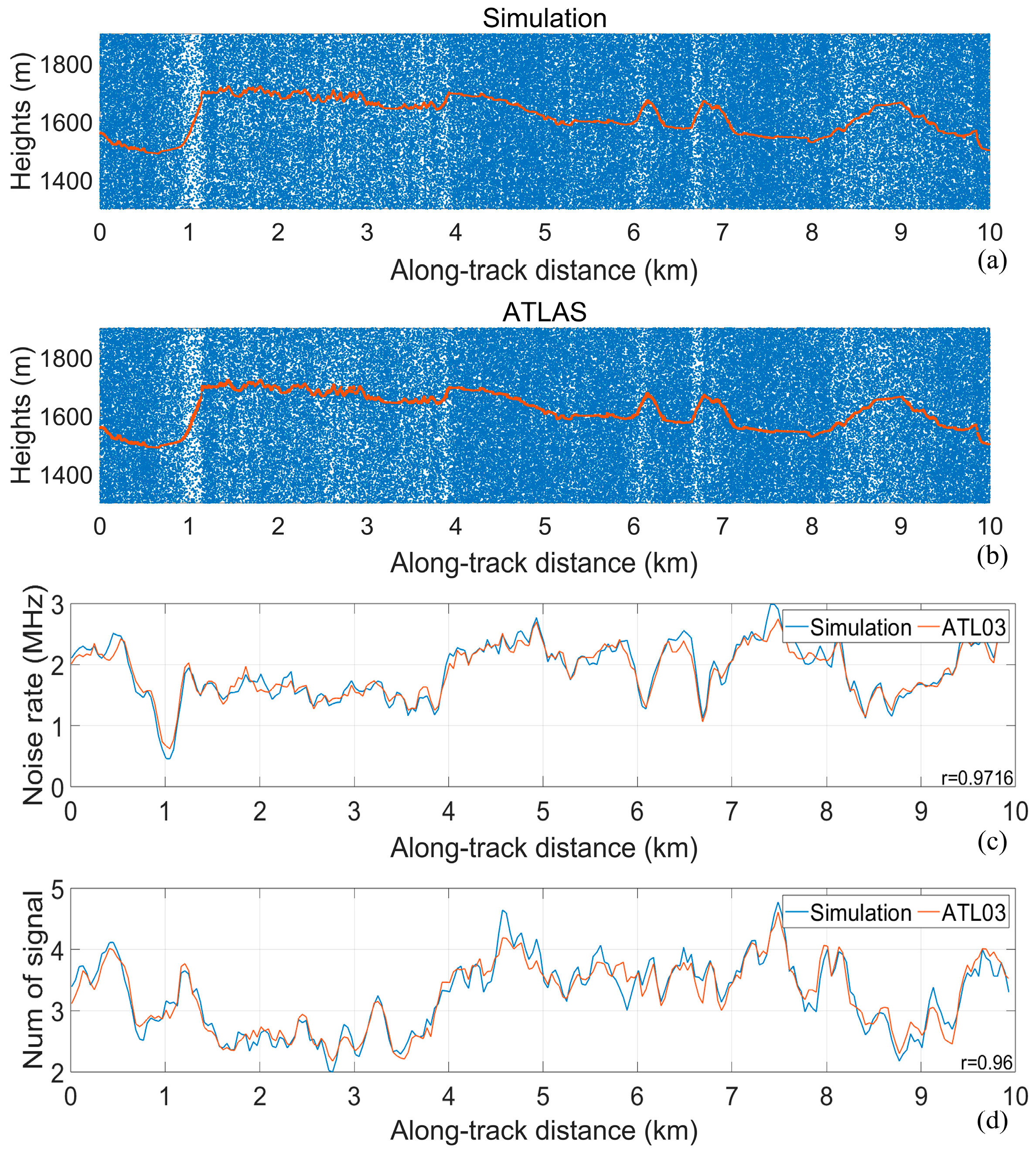
4.1. Validation of the Simulation Results

To validate the model proposed in this study, two tracks of simulation data, Data-s1 and Data-s2, were generated from ICESat-2 measured Data 1 (as shown in Figure 9a,b). The signal and noise distributions of Data 1 were used as inputs for Data-s1. Data1-s2 are simulated by fixing the echo signal strength and noise rate with an average signal photon count of 1 along the track with a noise rate of 5 MHz. In order to verify the correctness of the simulated point clouds, we counted the noise rate and signal photon number distributions along the track direction of Data-s1 and the measured point cloud (Figure 9c,d), where the correlation coefficients of the signal and noise distributions are 0.97 and 0.96, respectively, indicating a high degree of consistency between the simulated and measured data.

Next, the derived elevations of the simulated data were compared with those of the ICESat-2 data. Figure 10a,b show the elevation contour lines of the simulated and ICESat-2 point clouds. Figure 11 shows the scatter plot of the surface elevations of the simulated and ICESat-2 point clouds, with a correlation coefficient of 0.9995 and an RMSE of 1.03 m between the simulated and measured elevations.

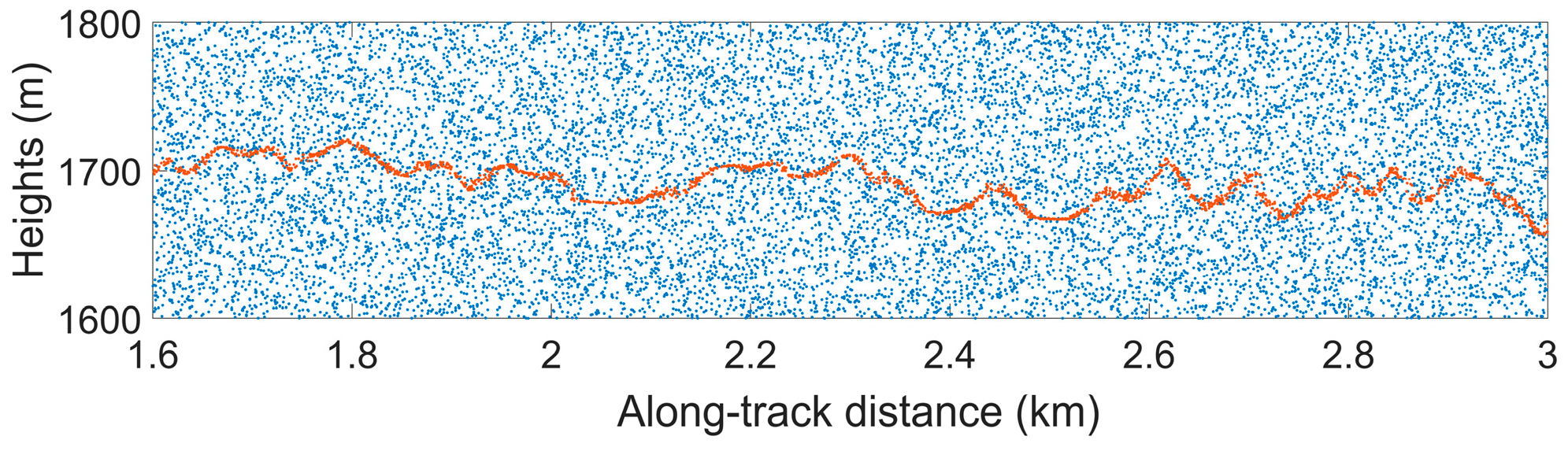
4.2. Validation of Feature Point Extraction

Figure 12 shows the feature point extraction results of the two-track simulation data, where the orange points are the feature points at the extraction. It can be seen that the feature points can basically reflect the distribution characteristics of the surface contour, although the feature points are somewhat intermittent in the along-track direction at a lower signal-to-noise ratio (Data-s2). To prove the reliability of the feature points for slope fitting, we use the linear fitting method to fit the slope to the simulated and feature point clouds, respectively, with a resolution of 30 m (The results are shown in Figure 13). The correlation coefficients between the slopes fitted to the two tracks of the simulation data and the slopes fitted to their corresponding feature points are 0.98 and 0.95, respectively.

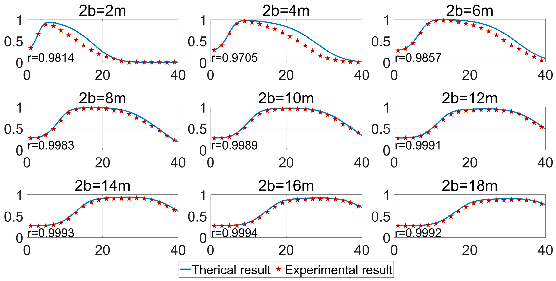
4.3. Validation of the PDF Model

Due to the variations in surface reflectivity and terrain relief, the distribution characteristics of signal and noise in the along-track direction are constantly changing. Validating the statistical model requires data with consistent distribution characteristics, which is challenging for long-distance ATL03 data in mountainous regions. This is because signal and noise distributions can only be approximated as consistent over shorter along-track distances. To address this, a segment of Data-s2 (1.6–3 km) was selected for PDF model validation. Data-s2 was simulated with a fixed average signal photon count and noise rate (Ns = 1, Nn = 5 MHz) The selected segment has a horizontal distribution range of 1400 m and an elevation distribution range of 200 m. The point cloud for this segment is shown in Figure 14.

Figure 15 compares the theoretical and experimental distributions of the F-score when the long axis is fixed at 10 m and the short axis takes different values (1–9 m). The red stars represent the experimental results, while the solid blue line represents the theoretical curve. The mean Pearson correlation coefficient r of the F-score is 0.9780, indicating excellent agreement between the theoretical and experimental results. Similarly, Figure 16 shows the theoretical and actual distributions of the F-score when the length of the long axis is fixed at 20 m and the short axis takes different values (2–18 m). The mean correlation coefficient r of the F-score is 0.9924.

The distribution of the maximum values of F-score for different search neighborhoods is shown in Figure 17, and its correlation coefficient r is 0.9, confirming the correctness of the proposed model. In the figure, we plotted the range of F equal to 0.9 and 0.95 using contour lines. However, variations in slope cause changes in pulse width over long distances, which increases the deviation between the theoretical calculations and the statistical results. To verify this point of view, we choose to shorten the length of data and use the point cloud of the first 400 m of the data for verification. Figure 18 shows the final results. The r of the F-score is 0.9697. The improved correlation between theoretical and statistical results further verifies the model’s accuracy and highlights the influence of pulse width consistency on the validation process.

5. Results

5.1. Results of Slope Estimation

The proposed feature point extraction algorithm was applied to the dataset, and the final results of the slope distribution between the slope fitted with feature points and the slope fitted with signal photons are shown in Figure 19, Figure 20 and Figure 21. The Pearson correlation coefficients r between the slopes fitted with feature points and the slopes fitted with signal photons were calculated for all the single-track data. r is basically above 0.9 for all the data used, and the value of r is only slightly reduced for very low signal-to-noise ratios (N_s = 1, f_n = 10 MHz). Figure 22 shows a scatter plot of the slope fitted using the feature points and the slope fitted using the labeled signal photons, with a correlation coefficient r of 0.9545 and a root mean square error RMSE of 5.26°, indicating that the slope can be accurately estimated using the extracted feature points.

While feature points demonstrate strong fidelity in capturing surface profile curvatures, some deviation exists between the slopes estimated using feature points and those estimated using the signal photons. These deviations arise because the feature points were selected based on the longest edge in the minimum spanning tree, which tends to pass near the center of the signal pulse width. As a result, the number of feature points is typically smaller than the number of signal photons, leading to slight inaccuracies in slope estimation. Additionally, the selected datasets are not entirely bare ground, and the presence of vegetation within the 30 m resolution segments can introduce some bias in slope estimation. Since a simple linear fit can achieve a correlation of more than 0.9, a more complex slope fitting method was not chosen for this study.

5.2. Denoising Results

To comprehensively evaluate the performance of the proposed denoising algorithm, simulated data, and ICESat-2 ATL03 data were used. For the simulated data, the ground truth signal values were determined during the simulation process. However, for the ATL03 data, the confidence labels provided are not always accurate. Therefore, manual labeling was performed based on the surface type confidence to obtain reliable ground truth values. The results of the proposed algorithm were compared with those of three other denoising algorithms, as well as with the ATL08 dataset. The denoising performance was quantitatively evaluated using three metrics: precision (Pre), recall (Rec), and F-score. The evaluation results are summarized in

Table 2. Denoising results of ATL03 data.

	Track Used	Quantitative Parameter	OPTICS	Quadtree	ATL08	Proposed Algorithm
Data 5	ATL03_20220421213643_ 04551506_005_02_GT3L	REC	0.9957	0.7908	0.9681	0.9301
		PRE	0.8372	0.8903	0.9119	0.9416
		F	0.9096	0.8376	0.9391	0.9358
Data 6	ATL03_20221001003812_ 01571706_005_01_GT2L	REC	0.9929	0.7661	0.7351	0.9292
		PRE	0.8727	0.9904	0.9640	0.9929
		F	0.9289	0.8639	0.8341	0.9600
Data 7	ATL03_20210926055926_ 00581302_005_01_GT2L	REC	0.9942	0.7964	0.8182	0.9030
		PRE	0.7244	0.7925	0.8091	0.9450
		F	0.8381	0.7945	0.8136	0.9235
Data 8	ATL03_20220613192251_ 12631506_005_01_GT2L	REC	0.9992	0.8079	0.9784	0.9136
		PRE	0.6707	0.7666	0.8440	0.9373
		F	0.8027	0.7867	0.9062	0.9253

and

Table 3. Denoising results of simulation data.

	NS	FN	Quantitative Parameter	OPTICS	Quadtree	DRAGANN	Proposed Algorithm
Data 2	1	0.5 MHZ	REC	0.9913	0.8932	0.9876	0.9816
			PRE	0.9152	0.9745	0.9145	0.9807
			F	0.9517	0.9321	0.9497	0.9812
		2 MHZ	REC	0.9841	0.8494	0.9440	0.9733
			PRE	0.8335	0.8890	0.8280	0.9218
			F	0.9026	0.8687	0.8822	0.9468
		10 MHZ	REC	0.9573	0.7929	0.9008	0.9049
			PRE	0.6737	0.6579	0.7765	0.8985
			F	0.7908	0.7191	0.8340	0.9017
	2	0.5 MHZ	REC	0.9847	0.8973	0.9960	0.9949
			PRE	0.9524	0.9764	0.9541	0.9887
			F	0.9683	0.9352	0.9746	0.9918
		2 MHZ	REC	0.9839	0.8552	0.9755	0.9908
			PRE	0.9048	0.9470	0.8939	0.9550
			F	0.9427	0.8988	0.9329	0.9726
		10 MHZ	REC	0.9730	0.8419	0.9691	0.9362
			PRE	0.7611	0.6050	0.7309	0.9328
			F	0.8541	0.7041	0.8333	0.9345
Data 3	0.64	0.5 MHZ	REC	0.9955	0.8044	0.9494	0.9252
			PRE	0.8575	0.9428	0.8233	0.9857
			F	0.9213	0.8681	0.8818	0.9545
		1 MHZ	REC	0.9915	0.8054	0.8859	0.8965
			PRE	0.7969	0.8595	0.7727	0.9752
			F	0.8836	0.8316	0.8255	0.9342
		2 MHZ	REC	0.9879	0.7816	0.9104	0.8803
			PRE	0.6780	0.6973	0.6824	0.9426
			F	0.8041	0.7371	0.7801	0.9104
Data 4	1.35	1 MHZ	REC	1	0.8947	0.9913	0.9973
			PRE	0.9225	0.9688	0.9225	0.9613
			F	0.9597	0.9303	0.9557	0.9789
		5 MHZ	REC	0.9976	0.8249	0.9847	0.9825
			PRE	0.8606	0.8690	0.7925	0.9295
			F	0.9240	0.8464	0.8782	0.9553
		10 MHZ	REC	0.9936	0.8337	0.9551	0.9773
			PRE	0.8438	0.6006	0.7372	0.9062
			F	0.9126	0.6982	0.8321	0.9404

. The proposed algorithm achieves an F-score greater than 0.9 even under very low signal-to-noise ratio (SNR) conditions, demonstrating its robustness and effectiveness.

6. Discussion

6.1. Analysis of Denoising Results

As shown in Figure 1, the track of Data 7 includes a segment of snow-covered mountains (located in the range of 7~10 km), and the acquisition time of this data is at noon in September, resulting in a low SNR and significant variations in noise level along the track, which increases the difficulty of denoising the point cloud. Figure 23 compares the denoising results of the proposed algorithm with those of three other methods (ATL08, quadtree, and OPTICS) for Data 7. The proposed algorithm demonstrates superior performance, particularly in challenging regions with low SNR and steep slopes.

To further analyze the denoising results, two 2 km long segments were selected from Data 7 and enlarged to be shown in Figure 24 and Figure 25. These segments include areas with slopes exceeding 40° and regions with snow cover (highlighted by green boxes). The results reveal that (1) the ATL08 algorithm is prone to signal leakage, resulting in broken signal profiles with steep slopes (e.g., 2 km in Figure 24c and 8.2 km in Figure 25c); (2) the quadtree algorithm struggles to reject locally dense noise photons and may miss sparser signal photons due to their shallow node positions in the quadtree structure (e.g., 1.4 km in Figure 24b and 8.2 km in Figure 25b); (3) the OPTICS algorithm has overall better performance, with a very high recall, but it may misclassify some noise photons in the vicinity of the signal as the signal; and (4) the algorithm proposed in this study has fewer outliers and breakpoints even in regions with weak signals and steep slopes, demonstrating its robustness.

The proposed algorithm employs optimal neighborhood and threshold values derived from theoretical calculations. This approach offers two key advantages: (1) Adaptive Parameter Selection: the algorithm can dynamically adjust parameters based on changes in point cloud slope, noise rate, and signal strength, ensuring optimal performance across varying conditions. (2) Accurate estimation of the slope: the algorithm can give the distribution of slopes in the along-track direction via MST-based slope estimation. This feature allows the algorithm to demonstrate superior performance in mountainous terrain.

6.2. The Robustness to Mislabeled Signal/Noise in Validation Datasets

To investigate the robustness to mislabeled signal/noise in validation datasets, we utilized one track of Data 2 to simulate mislabeling scenarios. As shown in Figure 26, the labeled signal photon count reached 6065, compared to the pre-labeled count of 5620 (indicating a 7.92% mislabeling rate). The denoising results are shown in

Table 4. Denoising results.

System Parameter	Pre	Rec	F
Truth	0.9218	0.9733	0.9468
Mislabeled	0.9234	0.9057	0.9147
Error	0.17%	6.95%	3.39%

.

Furthermore, the impact of mislabeling can be mathematically characterized as follows: let N denote the number of signal photons in the point cloud, NF represent the number of mislabeled photons, and NS indicate the total number of photons extracted by the denoising algorithm (where TP denotes correctly identified signal photons, FP corresponds to noise photons falsely classified as signal photons, and FN represents correctly identified noise photons). Under this framework, the authentic Precision (Pre), Recall (Rec), and F-score (F) can be expressed as follows:

$$\begin{array}{l}\mathrm{Pre}=TP/NS,\\ \mathrm{Rec}=TP/N,\\ \mathrm{F}={\displaystyle \frac{2\cdot \mathrm{Rec}\cdot \mathrm{Pre}}{\mathrm{Rec}+\mathrm{Pre}}},\end{array}$$

(23)

Under the influence of mislabeling effects, the evaluation metrics can be expressed as follows:

$$\begin{array}{l}{\mathrm{Pre}}_f=(TP+FP)/NS,\\ {\mathrm{Rec}}_f=(TP+FP)/(N+NF),\\ {\mathrm{F}}_f={\displaystyle \frac{2\cdot {\mathrm{Rec}}_f\cdot {\mathrm{Pre}}_f}{{\mathrm{Rec}}_f+{\mathrm{Pre}}_f}},\end{array}$$

(24)

The mathematical formulation reveals that mislabeling exerts a relatively minor influence on precision (Pre), while inducing more pronounced effects on recall (Rec). The systematic error in recall calculation attributable to mislabeling can be expressed as follows:

$$\Delta \mathrm{Rec}=|{\displaystyle \frac{TP+FP}{N+NF}}-{\displaystyle \frac{TP}{N}}|/({\displaystyle \frac{TP}{N}})\approx {\displaystyle \frac{NF}{N+NF}}={\displaystyle \frac{\Delta N}{1+\Delta N}},\Delta N={\displaystyle \frac{NF}{N}}.$$

(25)

The results demonstrate that when the ratio of mislabeled photons to signal photons remains below 10%, the computational error does not exceed 10%. The results clearly demonstrate that an 8% error (as shown in Figure 26) represents a substantial deviation which significantly exceeds the typical error range achievable through manual labeling (The error typically remains below 5%). Moreover, similar to many deep learning algorithms [58,59], manual annotations are conventionally adopted as ground truth. This quantitative comparison confirms the superior reliability of manual labeling.

7. Conclusions

This study presents an adaptive Bayesian denoising framework for low-SNR photon-counting Lidar data. Two primary contributions have been made: (1) an ATL03-based photon cloud simulation method was provided to generate different signal and noise levels with true labels for verifying and improving the denoising algorithms; and (2) dynamic parameter selection via MST-based slope estimation and probabilistic PDF modeling was performed, achieving F-scores > 0.9 even at 1 photon/10 MHz noise. Experimental results demonstrate 10% higher precision than ATL08, OPTICS, and Quadtree in steep terrain with low SNR, enabled by elliptical neighborhoods aligned with local slopes and optimized parameters in different SNR. The proposed algorithm can provide theoretical guidance for optimal parameter selection of point cloud denoising algorithms. Although the analytical expressions in this study are derived from the elliptic clustering algorithm, the underlying methodology of modeling probability density functions for signal and noise photon distributions may be extended to other approaches, such as selecting optimal thresholds in KNN methods or determining optimal pixel sizes in image-based denoising algorithms.

References

1. Markus, T.; Neumann, T.; Martino, A.; Abdalati, W.; Brunt, K.; Csatho, B.; Farrell, S.; Fricker, H.; Gardner, A.; Harding, D.; et al. The Ice, Cloud, and land Elevation Satellite-2 (ICESat-2): Science requirements, concept, and implementation. Remote Sens. Environ. 2017, 190, 260–273. [Google Scholar] [CrossRef]
2. Neumann, T.A.; Martino, A.J.; Markus, T.; Bae, S.; Bock, M.R.; Brenner, A.C.; Brunt, K.M.; Cavanaugh, J.; Fernandes, S.T.; Hancock, D.W.; et al. The Ice, Cloud, and Land Elevation Satellite-2 mission: A global geolocated photon product derived from the Advanced Topographic Laser Altimeter System. Remote Sens. Environ. 2019, 233, 111325. [Google Scholar] [CrossRef] [PubMed]
3. Smith, B.; Fricker, H.A.; Gardner, A.S.; Medley, B.; Nilsson, J.; Paolo, F.S.; Holschuh, N.; Adusumilli, S.; Brunt, K.; Csatho, B.; et al. Pervasive ice sheet mass loss reflects competing ocean and atmosphere processes. Science 2020, 368, 1239. [Google Scholar] [CrossRef]
4. Popescu, S.C.; Zhou, T.; Nelson, R.; Neuenschwande, A.; Sheridan, R.; Narine, L.; Walsh, K.M. Photon counting LiDAR: An adaptive ground and canopy height retrieval algorithm for ICESat-2 data. Remote Sens. Environ. 2018, 208, 154–170. [Google Scholar] [CrossRef]
5. Narine, L.L.; Popescu, S.; Neuenschwander, A.; Zhou, T.; Srinivasan, S.; Harbeck, K. Estimating aboveground biomass and forest canopy cover with simulated ICESat-2 data. Remote Sens. Environ. 2019, 224, 1–11. [Google Scholar] [CrossRef]
6. Fan, Y.; Ke, C.; Shen, X.; Xiao, Y.; Livingstone, S.J.; Sole, A.J. Subglacial lake activity beneath the ablation zone of the Greenland Ice Sheet. Cryosphere Discuss. 2022, 17, 1775–1786. [Google Scholar] [CrossRef]
7. Xu, Y.; Li, H.; Liu, B.; Xie, H.; Ozsoy Cicek, B. Deriving Antarctic sea-ice thickness from satellite altimetry and estimating consistency for NASA’s ICESat/ICESat-2 missions. Geophys. Res. Lett. 2021, 48, e2021GL093425. [Google Scholar] [CrossRef]
8. Feng, T.; Duncanson, L.; Montesano, P.; Hancock, S.; Minor, D.; Guenther, E.; Neuenschwander, A. A systematic evaluation of multi-resolution ICESat-2 ATL08 terrain and canopy heights in boreal forests. Remote Sens. Environ. 2023, 291, 113570. [Google Scholar] [CrossRef]
9. Zhu, X.X.; Nie, S.; Wang, C.; Xi, X.H.; Lao, J.Y.; Li, D. Consistency analysis of forest height retrievals between GEDI and ICESat-2. Remote Sens. Environ. 2022, 281, 113244. [Google Scholar] [CrossRef]
10. Martino, A.J.; Neumann, T.A.; Kurtz, N.T.; Mclennan, D. ICESat-2 mission overview and early performance. In Proceedings of the Sensors, Systems, and Next-Generation Satellites XXIII, Strasbourg, France, 9–12 September 2019; pp. 68–77. [Google Scholar]
11. Magruder, L.A.; Brunt, K.M.; Alonzo, M. Early ICESat-2 on-orbit geolocation validation using ground-based corner cube retro-reflectors. Remote Sens. 2020, 12, 3653. [Google Scholar] [CrossRef]
12. Parrish, C.E.; Magruder, L.A.; Neuenschwander, A.L.; Forfinski-Sarkozi, N.; Alonzo, M.; Jasinski, M. Validation of ICESat-2 ATLAS Bathymetry and Analysis of ATLAS’s Bathymetric Mapping Performance. Remote Sens. 2019, 11, 1634. [Google Scholar] [CrossRef]
13. Ranndal, H.; Sigaard Christiansen, P.; Kliving, P.; Baltazar Andersen, O.; Nielsen, K. Evaluation of a statistical approach for extracting shallow water bathymetry signals from ICESat-2 ATL03 photon data. Remote Sens. 2021, 13, 3548. [Google Scholar] [CrossRef]
14. Lee, Z.; Shangguan, M.; Garcia, R.A.; Lai, W.; Lu, X.; Wang, J.; Yan, X. Confidence measure of the shallow-water bathymetry map obtained through the fusion of Lidar and multiband image data. J. Remote Sens. 2021, 2021, 9841804. [Google Scholar] [CrossRef]
15. Franze, S.E.; Andersen, O.B.; Nilsson, B.; Nielsen, K. Lake gravity anomalies from ICESat-2 laser altimetry and geodetic radar altimetry. Adv. Space Res. 2024, 74, 4487–4501. [Google Scholar] [CrossRef]
16. Horvat, C.; Blanchard Wrigglesworth, E.; Petty, A. Observing waves in sea ice with ICESat-2. Geophys. Res. Lett. 2020, 47, e2020GL087629. [Google Scholar] [CrossRef]
17. Bagnardi, M.; Kurtz, N.T.; Petty, A.A.; Kwok, R. Sea Surface Height Anomalies of the Arctic Ocean from ICESat-2: A First Examination and Comparisons with CryoSat-2. Geophys. Res. Lett. 2021, 48, e2021GL093155. [Google Scholar] [CrossRef]
18. Herzfeld, U.; Hayes, A.; Palm, S.; Hancock, D.; Vaughan, M.; Barbieri, K. Detection and Height Measurement of Tenuous Clouds and Blowing Snow in ICESat-2 ATLAS Data. Geophys. Res. Lett. 2021, 48, e2021GL093473. [Google Scholar] [CrossRef]
19. Palm, S.P.; Yang, Y.K.; Herzfeld, U.; Hancock, D.; Hayes, A.; Selmer, P.; Hart, W.; Hlavka, D. ICESat-2 Atmospheric Channel Description, Data Processing and First Results. Earth Space Sci. 2021, 8, e2020EA001470. [Google Scholar] [CrossRef]
20. Palm, S.P.; Selmer, P.; Yorks, J.; Nicholls, S.; Nowottnick, E. Planetary Boundary Layer Height Estimates from ICESat-2 and CATS Backscatter Measurements. Front. Remote Sens. 2021, 2, 716951. [Google Scholar] [CrossRef]
21. Xu, N.; Ma, Y.; Zhou, H.; Zhang, W.; Zhang, Z.; Wang, X.H. A method to derive bathymetry for dynamic water bodies using ICESat-2 and GSWD data sets. IEEE Geosci. Remote Sens. Lett. 2020, 19, 1500305. [Google Scholar] [CrossRef]
22. Winker, D.M.; Vaughan, M.A.; Omar, A.; Hu, Y.; Powell, K.A.; Liu, Z.; Hunt, W.H.; Young, S.A. Overview of the CALIPSO mission and CALIOP data processing algorithms. J. Atmos. Ocean. Technol. 2009, 26, 2310–2323. [Google Scholar] [CrossRef]
23. Palm, S.P.; Yang, Y.U.; Herzfeld, C. ICESat-2 Algorithm Theoretical Basis Document for Atmospheric Data Products (ATL04 & ATL09), version 8.3; Technical Report; NASA National Snow and Ice Data Center, Distributed Active Archive Center: Washington, DC, USA, 2020. [Google Scholar]
24. Yang, J.; Zheng, H.Y.; Ma, Y.; Zhao, P.F.; Zhou, H.; Li, S.; Wang, X.H. Background noise model of spaceborne photon-counting lidars over oceans and aerosol optical depth retrieval from ICESat-2 noise data. Remote Sens. Environ. 2023, 299, 113858. [Google Scholar] [CrossRef]
25. Abshire, J.B.; Sun, X.; Riris, H.; Sirota, J.M.; Mcgarry, J.F.; Palm, S.; Yi, D.; Liiva, P. Geoscience laser altimeter system (GLAS) on the ICESat mission: On-orbit measurement performance. Geophys. Res. Lett. 2005, 32, 21–22. [Google Scholar] [CrossRef]
26. Horan, K.H.; Kerekes, J.P. An automated statistical analysis approach to noise reduction for photon-counting lidar systems. In Proceedings of the 2013 IEEE International Geoscience and Remote Sensing Symposium-IGARSS, Melbourne, Australia, 21–26 July 2013; pp. 4336–4339. [Google Scholar]
27. Luthcke, S.B.; Pennington, T.; Rebold, T.; Thomas, T. Algorithm Theoretical Basis Document (ATBD) for ATL03g ICESat-2 Receive Photon Geolocation; NASA Goddard Space Flight Center: Greenbelt, MD, USA, 2019; p. 53. [Google Scholar]
28. Neuenschwander, A.; Pitts, K. The ATL08 land and vegetation product for the ICESat-2 Mission. Remote Sens. Environ. 2019, 221, 247–259. [Google Scholar] [CrossRef]
29. Wang, X.; Pan, Z.G.; Glennie, C. A Novel Noise Filtering Model for Photon-Counting Laser Altimeter Data. IEEE Geosci. Remote Sens. Lett. 2016, 13, 947–951. [Google Scholar] [CrossRef]
30. Ma, R.J.; Kong, W.; Chen, T.; Shu, R.; Huang, G.H. KNN Based Denoising Algorithm for Photon-Counting LiDAR: Numerical Simulation and Parameter Optimization Design. Remote Sens. 2022, 14, 6236. [Google Scholar] [CrossRef]
31. Zhang, J.; Kerekes, J.; Csatho, B.; Schenk, T.; Wheelwright, R. A clustering approach for detection of ground in micropulse photon-counting LiDAR altimeter data. In Proceedings of the 2014 IEEE Geoscience and Remote Sensing Symposium, Quebec City, QC, Canada, 13–18 July 2014; pp. 177–180. [Google Scholar]
32. Zhang, J.S.; Kerekes, J. An Adaptive Density-Based Model for Extracting Surface Returns from Photon-Counting Laser Altimeter Data. IEEE Geosci. Remote Sens. Lett. 2015, 12, 726–730. [Google Scholar] [CrossRef]
33. Ester, M.; Kriegel, H.; Sander, J.; Xu, X. A density-based algorithm for discovering clusters in large spatial databases with noise. In Proceedings of the KDD-96: The Second International Conference on Knowledge Discovery and Data Mining, Miinchen, Germany, 2 August 1996; pp. 226–231. [Google Scholar]
34. Ma, Y.; Zhang, W.; Sun, J.; Li, G.; Wang, X.H.; Li, S.; Xu, N. Photon-counting Lidar: An adaptive signal detection method for different land cover types in coastal areas. Remote Sens. 2019, 11, 471. [Google Scholar] [CrossRef]
35. Huang, J.; Xing, Y.; You, H.; Qin, L.; Tian, J.; Ma, J. Particle swarm optimization-based noise filtering algorithm for photon cloud data in forest area. Remote Sens. 2019, 11, 980. [Google Scholar] [CrossRef]
36. Zhang, J. Analytical Modeling and Performance Assessment of Micropulse Photon-Counting Lidar System; Rochester Institute of Technology: Rochester, NY, USA, 2014; ISBN 1321453779. [Google Scholar]
37. Nie, S.; Wang, C.; Xi, X.; Luo, S.; Li, G.; Tian, J.; Wang, H. Estimating the vegetation canopy height using micro-pulse photon-counting LiDAR data. Opt. Express 2018, 26, A520–A540. [Google Scholar] [CrossRef]
38. Zhang, Z.Y.; Liu, X.Y.; Ma, Y.; Xu, N.; Zhang, W.H.; Li, S. Signal Photon Extraction Method for Weak Beam Data of ICESat-2 Using Information Provided by Strong Beam Data in Mountainous Areas. Remote Sens. 2021, 13, 863. [Google Scholar] [CrossRef]
39. Zhu, X.X.; Nie, S.; Wang, C.; Xi, X.H.; Wang, J.S.; Li, D.; Zhou, H.Y. A Noise Removal Algorithm Based on OPTICS for Photon-Counting LiDAR Data. IEEE Geosci. Remote Sens. Lett. 2021, 18, 1471–1475. [Google Scholar] [CrossRef]
40. Zhang, G.P.; Xu, Q.; Xing, S.; Li, P.C.; Zhang, X.L.; Wang, D.D.; Dai, M.F. A Noise-Removal Algorithm Without Input Parameters Based on Quadtree Isolation for Photon-Counting LiDAR. IEEE Geosci. Remote Sens. Lett. 2022, 19, 1–5. [Google Scholar] [CrossRef]
41. Neumann, T.; Brenner, A.; Hancock, D.; Robbins, J.; Saba, J.; Harbeck, K.; Gibbons, A. ICE, CLOUD, and Land Elevation Satellite-2 (ICESat-2) Project Algorithm Theoretical Basis Document (ATBD) for Global Geolocated Photons ATL03; National Aeronautics and Space Administration, Goddard Space Flight Center: Greenbelt, MD, USA, 2019. [Google Scholar]
42. Neumann, T.A.; Brenner, A.; Hancock, D.; Robbins, J.; Saba, J.; Harbeck, K.; Gibbons, A.; Lee, J.; Luthcke, S.B.; Rebold, T. ATLAS/ICESat-2 L2A Global Geolocated Photon Data, version 3; NASA National Snow and Ice Data Center Distributed Active Archive Center: Boulder, CO, USA, 2021. [Google Scholar]
43. Neuenschwander, A.L.; Pitts, K.L.; Jelley, B.P.; Robbins, J.; Klotz, B.; Popescu, S.C.; Nelson, R.F.; Harding, D.; Pederson, D.; Sheridan, R. ATLAS/ICESat-2 L3A Land and Vegetation Height, version 3; NASA National Snow and Ice Data Center Distributed Active Archive Center: Boulder, CO, USA, 2021. [Google Scholar]
44. Malambo, L.; Popescu, S. Photonlabeler: An inter-disciplinary platform for visual interpretation and labeling of icesat-2 geolocated photon data. Remote Sens. 2020, 12, 3168. [Google Scholar] [CrossRef]
45. Gardner, C.S. Target Signatures for Laser Altimeters—An analysis. Appl. Opt. 1982, 21, 448–453. [Google Scholar] [CrossRef]
46. Gardner, C.S. Ranging performance of satellite laser altimeters. IEEE Trans. Geosci. Remote Sens. 1992, 30, 1061–1072. [Google Scholar] [CrossRef]
47. Degnan, J.J. Photon-counting multikilohertz microlaser altimeters for airborne and spaceborne topographic measurements. J. Geodyn. 2002, 34, 503–549. [Google Scholar] [CrossRef]
48. Liu, X.; Ma, Y.; Li, S.; Yang, J.; Zhang, Z.; Tian, X. Photon counting correction method to improve the quality of reconstructed images in single photon compressive imaging systems. Opt. Express 2021, 29, 37945–37961. [Google Scholar] [CrossRef]
49. Li, S.; Liu, X.; Xiao, Y.; Ma, Y.; Yang, J.; Zhu, K.; Tian, X. 3D compressive imaging system with a single photon-counting detector. Opt. Express 2023, 31, 4712–4738. [Google Scholar] [CrossRef]
50. Müller, J.W. Dead-time problems. Nucl. Instrum. Methods 1973, 112, 47–57. [Google Scholar] [CrossRef]
51. Gatt, P.; Johnson, S.; Nichols, T. Geiger-mode avalanche photodiode ladar receiver performance characteristics and detection statistics. Appl. Opt. 2009, 48, 3261–3276. [Google Scholar] [CrossRef] [PubMed]
52. Zhang, Z.; Ma, Y.; Li, S.; Zhao, P.; Xiang, Y.; Liu, X.; Zhang, W. Ranging performance model considering the pulse pileup effect for PMT-based photon-counting lidars. Opt. Express 2020, 28, 13586–13600. [Google Scholar] [CrossRef]
53. Ma, Y.; Li, S.; Zhang, W.; Zhang, Z.; Liu, R.; Wang, X.H. Theoretical ranging performance model and range walk error correction for photon-counting lidars with multiple detectors. Opt. Express 2018, 26, 15924–15934. [Google Scholar] [CrossRef]
54. Marpaung, F.; Arnita. Comparative of prim’s and boruvka’s algorithm to solve minimum spanning tree problems. J. Phys. Conf. Ser. 2020, 1462, 012043. [Google Scholar] [CrossRef]
55. Sedgewick, R.; Wayne, K. Algorithms; Addison-Wesley Professional: Boston, MA, USA, 2011; ISBN 032157351X. [Google Scholar]
56. Gelman, A.; Carlin, J.B.; Stern, H.S.; Rubin, D.B. Bayesian Data Analysis; Chapman and Hall/CRC: Boca Raton, FL, USA, 1995; ISBN 0429258410. [Google Scholar]
57. Hripcsak, G.; Rothschild, A.S. Agreement, the f-measure, and reliability in information retrieval. J. Am. Med. Inf. Assoc. 2005, 12, 296–298. [Google Scholar] [CrossRef] [PubMed]
58. Lin, Y.; Knudby, A.J. Global automated extraction of bathymetric photons from icesat-2 data based on a pointnet++ model. Int. J. Appl. Earth Obs. Geoinf. 2023, 124, 103512. [Google Scholar] [CrossRef]
59. Velikova, M.; Fernandez-Diaz, J.; Glennie, C. ICESat-2 noise filtering using a point cloud neural network. ISPRS Open J. Photogramm. Remote Sens. 2024, 11, 100053. [Google Scholar] [CrossRef]
Figure 1. Overview of the experimental areas. (a) Eastern Utah. (b,c) Altun Mountain in Tibet. (d) Southern Nevada.
Remotesensing 17 02182 g001
Figure 2. Generation process of simulation point clouds for a photon-counting Lidar.
Remotesensing 17 02182 g002
Figure 3. Point clouds generated using DSM simulation based on the Data 1 trajectory. (a) Ns = 1, Nn = 0.5 MHz; (b) Ns = 1, Nn = 2 MHz; (c) Ns = 1, Nn = 10 MHz; (d) Ns = 2, Nn = 0.5 MHz; (e) Ns = 2, Nn = 2 MHz; (f) Ns = 2, Nn = 10 MHz.
Remotesensing 17 02182 g003
Figure 4. Simulated point clouds generated from ATL03 data. (ac) are generated based on Data 2. (df) are generated based on Data 3. (a) Nn = 0.5 MHz; (b) Nn = 1 MHz; (c) Nn = 2 MHz; (d) Nn = 1 MHz; (e) Nn = 5 MHz; (f) Nn = 10 MHz.
Remotesensing 17 02182 g004
Figure 5. ICESat-2 weak-beam data in the test dataset. (a) Data5; (b) data6; (c) data7; (d) data8.
Remotesensing 17 02182 g005
Figure 6. Positions of the six classes of photons in the point cloud. (a) Noise region; (b) signal region.
Remotesensing 17 02182 g006
Figure 7. Schematic diagram of the hierarchical model of the signal region.
Remotesensing 17 02182 g007
Figure 8. The flowchart for the denoising algorithm.
Remotesensing 17 02182 g008
Figure 9. (a,b) are the simulated and measured point cloud, (c) is the noise rate distribution of the point cloud in the along-track direction, and (d) is the signal distribution of the point cloud in the along-track direction.
Remotesensing 17 02182 g009
Figure 10. (a,b) are the signal elevation contour lines of the simulated and ICESat-2 point clouds.
Remotesensing 17 02182 g010
Figure 11. The scatter plot of the surface elevations of the simulated and ICESat-2 point clouds.
Remotesensing 17 02182 g011
Figure 12. The feature point extraction results of Data-s1 and Data-s2. (a) Feature point extraction results of Data-s1; (b) feature point extraction results of Data-s2.
Remotesensing 17 02182 g012
Figure 13. The results of slope estimation. (a) Slope estimation results of Data-s1; (b) slope estimation results of Data-s2.
Remotesensing 17 02182 g013
Figure 14. Simulated point cloud for model validation.
Remotesensing 17 02182 g014
Figure 15. Theoretical and experimental results of F-score of Data-s1 for long axis value of 10 m.
Remotesensing 17 02182 g015
Figure 16. Theoretical and experimental results of F-score of Data-s1 for long axis value of 20 m.
Remotesensing 17 02182 g016
Figure 17. Distribution of maximum values of F corresponding to different search neighborhoods (1400 m). (a) Theoretical result; (b) experimental result.
Remotesensing 17 02182 g017
Figure 18. Distribution of maximum values of F corresponding to different search neighborhoods (400 m). (a) Theoretical result; (b) experimental result.
Remotesensing 17 02182 g018
Figure 19. Slope estimation results for simulated point clouds.
Remotesensing 17 02182 g019
Figure 20. Slope estimation results for ATL03-simulation point cloud. (ac) are the results of Data 2. (df) are the results of Data 3. (a) Nn = 0.5 MHz; (b) Nn = 1 MHz; (c) Nn = 2 MHz; (d) Nn = 1 MHz; (e) Nn = 5 MHz; (f) Nn = 10 MHz.
Remotesensing 17 02182 g020
Figure 21. Slope estimation results for ATL03 data. (a) Data5; (b) data6; (c) data7; (d) data8.
Remotesensing 17 02182 g021
Figure 22. Scatterplot of slope estimation.
Remotesensing 17 02182 g022
Figure 23. Denoising results of four methods for Data 6.
Remotesensing 17 02182 g023
Figure 24. Local enlargement of the denoising results in the region corresponding to the orange box. (a) OPTICS; (b) Quadtree; (c) ATL08; (d) Our method.
Remotesensing 17 02182 g024
Figure 25. Local enlargement of the denoising results in the region corresponding to the green box. (a) OPTICS; (b) Quadtree; (c) ATL08; (d) Our method.
Remotesensing 17 02182 g025
Figure 26. Result of mislabeling.
Remotesensing 17 02182 g026