Article

A Unified Multi-Target Clever Eye Algorithm: Analytical Solutions and Application

by
Lei Wang
1,
Xiurui Geng
2,3,4,* and
Luyan Ji
2,4
1
The School of Microelectronics and Communication Engineering, Chongqing University, Chongqing 400044, China
2
Aerospace Information Research Institute, Chinese Academy of Sciences, Beijing 100094, China
3
The School of Electronic, Electrical and Communication Engineering, University of the Chinese Academy of Sciences, Beijing 100049, China
4
The Key Laboratory of Technology in Geo-Spatial Information Processing and Application System, Chinese Academy of Sciences, Beijing 100864, China
*
Author to whom correspondence should be addressed.
Remote Sens. 2025, 17(13), 2148; https://doi.org/10.3390/rs17132148
Submission received: 24 March 2025 / Revised: 24 May 2025 / Accepted: 29 May 2025 / Published: 23 June 2025

Abstract

The clever eye (CE) algorithm has been introduced for target detection in remote sensing image processing. It originally proposes the concept of data origin and can achieve the lowest average output energy compared to both the classical constrained energy minimization (CEM) and matched filter (MF) methods. In addition, it has been theoretically proven that the solutions of the best data origins can be attributed to solving a linear equation, which makes it computationally efficient. However, CE is only designed for single-target detection cases, while multiple-target detection is more demanding in real applications. In this paper, by naturally extending CE to a multiple-target case, we propose a unified algorithm termed multi-target clever eye (MTCE). The theoretical results in CE prompt us to consider an interesting question: do the MTCE solutions also share a similar structure to those of CE? Aiming to answer this question, we investigate a class of unconstrained non-convex optimization problems, where both the CE and MTCE models serve as special cases, which, interestingly, can also be utilized to solve a more generalized linear system. In addition, we further prove that all these solutions are globally optimal. In this sense, the analytical solutions of this generalized model can be deduced. Therefore, a unified framework is provided to deal with such a non-convex optimization problem, where both the solutions of MTCE and CE can be succinctly derived. Furthermore, its computational complexity is of the same magnitude as that of the other multiple-target-based methods. Experiments on both simulations and real hyperspectral remote sensing data verify our theoretical conclusions, and the comparison of quantitative metrics also demonstrates the advantage of our proposed MTCE method in multiple-target detection.

1. Introduction

Since remote sensing imagery consists of tens or hundreds of bands with a very high spectral resolution, it has prompted the development of various applications over the past decades. Target detection is one of the most important tasks in the field of remote sensing image processing, which aims to detect and highlight the specified target of interest and to distinguish it from the background pixels within a given environment or dataset. This task has a broad range of real applications, such as camouflage target detection [1], agricultural production [2], land use [3], climate change [4], urban monitoring [5], ship detection [6], etc.
Currently, existing target detection methods can be divided into the following four categories: (1) Algorithms based on the spectral similarity index, which aim to calculate the spectral difference between the target and background pixels. The most commonly used one is the spectral angle mapping [7]; (2) Linear mixing model (LMM)-based algorithms, which assume that any mixed pixel can be regarded as a linear combination of endmembers that can be viewed as targets of interest [8]. The represented algorithms are orthogonal subspace projection [9,10], and non-negative matrix factorization [11,12]; (3) Learning-based algorithms, such as multitasking and metric learning [13,14,15,16]. (4) Algorithms based on statistical metrics. Currently, the second-order statistic is widely applied, and the classical methods include constrained energy minimization (CEM) [17] and the matched filter (MF) method [18]; except for the second-order statistic, higher-order statistics have also been introduced for this task [19,20]. In recent years, deep learning-based methods such as [21,22,23,24,25,26,27] have emerged and been developed for target detection tasks.
However, they require supervised pre-training via a large number of labeled samples to learn good representation and thus also suffer from a high computational burden. In this paper, we will focus on the last class for discussion, which can be grouped into the unsupervised learning type. As opposed to the deep learning class, this branch does not require a pre-training process and has received more attention in small-sample scenarios.
The most classical statistic-based target detection algorithm is CEM, which was developed from the field of signal processing. To detect targets of interest, it aims to find a projection direction to keep the output of the target as a constant while suppressing the average filter output energy of the data to a minimum level. In this way, the target can be highlighted. Though MF is designed from the perspective of the binary statistical hypothesis, the MF detector is very similar to that of CEM, only differing in that the data should first be centralized for MF. From the perspective of the optimization model, both of them can be viewed as a convex optimization model with a linear constraint. Formally, a convex function is defined as follows: let f be a function defined on a subset I of the real numbers R . If for all x 1 , x 2 I and for all t [ 0 , 1 ] , the following inequality holds, f ( t x 1 + ( 1 t ) x 2 ) t f ( x 1 ) + ( 1 t ) f ( x 2 ) , then the function f is said to be convex on the interval I. However, they have different levels of performance, caused by the change of the data’s origin. This means that the selection of the data’s origin will have an impact on the performance of target detection.
In this sense, the clever eye (CE) algorithm, which originally introduces the concept of the data’s origin as a new variable, has been proposed, where both CEM and MF can be viewed as special cases [28]. Compared to CEM and MF, there are two coupled variables to be optimized in the CE model, leading to a non-convex optimization model. In [28], the authors adopted an iterative gradient method in order to obtain a feasible solution. More interestingly, after rigid theoretical analysis, the non-convex optimization model of CE can be attributed to solving a system of linear equations. Meanwhile, they further show that all of these stationary points are globally optimal [29] (see Theorems 1 and 2 later for details). In this sense, there exist analytical solutions for CE, making it computationally efficient and also theoretically guaranteed.
However, the above model is only limited to single-target detection tasks, and may not satisfy demands in real applications. Therefore, previous works have extended some models to multiple-target cases, including both linear and non-linear types. For the linear class, multi-target CEM (MTCEM) and multi-target MF (MTMF) can be easily generalized in a natural way. The non-linear type incorporates some non-linear operations into target detection, such as Sum CEM (SCEM) [30], Winner-Takes-All CEM (WTACEM) [30], and Revised MTCEM (RMTCEM) [31]. Following the linear class, the CE model can also be extended into multiple-target cases, which is considered and analyzed in this work and is termed the multi-target CE (MTCE) algorithm for consistency. Inspired by theoretical results in CE, we consider an interesting question: do the MTCE solutions also share a similar structure to those of CE? In this paper, we investigate this issue and establish a theoretical analysis of it. Then, we evaluate the performance of MTCE in target detection tasks for a remote sensing dataset.
The rest of this paper is organized as follows. In Section 2, we briefly review some classical algorithms and present existing theoretical results for CE. In Section 3, we propose the generalized MTCE model and derive its simplified model. In Section 4, we give a detailed theoretical analysis of a class of unconstrained non-convex models, where both the CE and MTCE models are classed as special cases. Finally, the computational complexity of MTCE is also presented. Some experimental results that focus on the application of MTCE in target detection are given in Section 5. The conclusions and some possible future works are presented in Section 6.

2. Preliminaries

In this part, we introduce several classical algorithms for target detection tasks and discuss existing theoretical results for CE. For intuition, the notations used in this article are defined in Table 1.

2.1. CEM

CEM comes from linear constrained minimum variance beamforming in the field of digital signal processing, which was proposed by Harsanyi in 1993. It has also become one of the most important target detection methods in the field of remote sensing image processing [17]. Mathematically, it is designed to find a direction w in order to minimize the average output energy of the data projected along w while keeping the output of the target of interest constant. We denote the hyperspectral (or multispectral) data T = [ t 1 , t 2 , , t N ] R L × N , where L , N are the number of bands and pixels, respectively. d = [ d 1 , d 2 , , d L ] T R L × 1 is the target vector to be detected. The CEM model is
min w 1 N ( i = 1 N y i 2 ) = min w w T R w s . t . d T w = 1 ,
where y i = w T t i , R = 1 N i = 1 N t i t i T is the correlation matrix of T . (1) is a quadratic convex model with an equality constraint. By using the Lagrangian method, the solution of (1) can be obtained by w = R 1 d d T R 1 d . Then, the objective function is calculated by
f ( w ) = w T R w = 1 d T R 1 d .
The CEM output is given by
y = w T T = d T R 1 d T R 1 d T

2.2. Multi-Target CEM (MTCEM)

CEM is only designed for single- target detection situations. However, in many scenarios, multiple-target detection applications are more demanding. In this way, multi-target CEM (MTCEM) is proposed by adding more target signatures to the CEM constraint. We assume that D p = [ d 1 , d 2 , , d p ] R L × p is a p target spectrum selected from N ones, where p L in general. Then, the MTCEM model is
min w 1 N ( i = 1 N y i 2 ) = min w w T R w s . t . D p T w = 1 p ,
where 1 p R p × 1 is a vector with all of the elements equal to 1. By similarly using the Lagrangian method, the solution of (4) can be obtained:
w MTCEM = R 1 D p ( D p T R 1 D p ) 1 1 p ,

2.3. Clever Eyes (CE) Algorithm

It is easy to find that the performance of CEM is influenced by the selection of the data’s origin, and different origins usually lead to different results. To search for the best data origin, an algorithm termed the clever eyes (CE) algorithm is proposed. It simultaneously finds the optimal data origin (denoted u ) and the projection direction w to minimize the average output energy of the data projected along w at position u and to maintain the output of the selected samples d at a constant. The model of CE is formulated as [28]
min w , u 1 N ( i = 1 N z i 2 ) = min w , u w T R u w s . t . ( d u ) T w = 1 ,
where z i = w T ( t i u ) , and
R u = 1 N [ i = 1 N ( t i u ) ( t i u ) T ] = K + ( m u ) ( m u ) T ,
where m = 1 N i = 1 N t i is the mean vector of T , and
K = 1 N [ i = 1 N ( t i m ) ( t i m ) T ]
is the covariance matrix of T . Similarly, by introducing the Lagrangian method, the filter vector corresponding to (6) can be obtained:
w CE = R u 1 ( d u ) ( d u ) T R u 1 ( d u ) .
Then, the objective function in (6) is transformed into
f ( u ) = w CE T R u w CE = 1 ( d u ) T R u 1 ( d u ) ,
Since the numerator is a constant, equivalently, minimizing (10) is transformed into maximizing the following function:
max u g ( u ) = ( d u ) T R u 1 ( d u ) .
The solution of (11) is called the best data origin.

2.4. The Analytical Solutions of CE

With rigid theoretical analysis, it has been proven that searching for the stationary points of (11) is similar to solving a system of linear equations, which makes the CE algorithm computationally efficient. Meanwhile, theoretical results show that all of these stationary points are globally optimal. The results are presented as the following two theorems.
Theorem 1 
([29]). To achieve the optimal target detector from the perspective of the filter output energy, the target vector, d ; data mean vector, m ; the data covariance matrix, K ; and data origin, u must satisfy the following linear equation (represented in the matrix form):
( d m ) T K 1 ( m u ) = 1 ,
which is named the clever eye equation.
Theorem 2 
([29]). For any u that satisfies the clever eye Equation (10) or (11), the corresponding detector and filter output energy are both u -irrelevant, which are
w CE = K 1 ( d m ) ( d m ) T K 1 ( d m ) + 1 ,
g ( u ) = ( d m ) T K 1 ( d m ) + 1 .

3. Unified Multi-Target CE (MTCE)

3.1. Model Formulation

Similar to extending CEM into MTCEM, it is natural to generalize CE to the multi-target case, which is termed the multi-target CE (MTCE) algorithm and is better adapted to real applications. In the following, we will focus on this algorithm and further derive its simplified version.
More specifically, the MTCE model is intended to simultaneously find a data origin direction u and a projection one w to minimize the variance of the data projected along w when observing the data “standing” at u and also to maintain the output of the selected samples D p at a constant. And it can be formulated as follows:
min w , u 1 N ( i = 1 N η i 2 ) = min w , u w T R u w ( D p u l p T ) T w = l p ,
in which, η i = w T ( t i u ) , and R u is defined in (7).
It should be noted that MTCEM can be viewed as a case of MTCE when the data origin is set to u = 0 , and MTMF can be viewed as a case of MTCE when u = m . CE can be viewed as a case of MTCE when p = 1 . Furthermore, when u = 0 and p = 1 , it is classed as a CEM model. When u = m and p = 1 , it is classed as an MF model. Thus, the proposed MTCE model provides a more unified framework which can incorporate many presented models as its special cases. An intuitive table is provided in Table 2.

3.2. Model Simplication

The Lagrangian function of (15) is defined as
f ( w , u ) = 1 2 w T R u w + Λ T [ l p ( D p u l p T ) T w ] ,
where Λ R p × 1 is the Lagrangian multiplier. By firstly fixing u , the gradient f w = 0 leads to
w u = R u 1 ( D p u l p T ) Λ ,
where we use the subscript to indicate that w is a function of u . Substituting (17) into the constraint in (15), it follows that
( D p u l p T ) T R u 1 ( D p u l p T ) Λ = l p ,
Λ = [ ( D p u l p T ) T R u 1 ( D p u l p T ) ] 1 l p .
Thus, the MTCE detector w u is given by
w u = R u 1 ( D p u l p T ) [ ( D p u l p T ) T R u 1 ( D p u l p T ) ] 1 l p .
and the objective function in (15) can be transformed into
min u f ( u ) = w u T R u w u = l p T [ ( D p u l p T ) T R u 1 ( D p u l p T ) ] 1 l p .
The solution of (21) is the best data origin (denoted u * ) for the MTCE model.
Motivated by the theoretical results in the CE model, as presented in Theorems 1 and 2, we were inspired to consider the following interesting question: as MTCE is a more generalized version of CE, do the solutions of the MTCE model also have a similar structure to that of the CE algorithm? In this paper, we focus on this question and provide a positive answer to it.
Note that the MTCE model is more complicated than that of CE, since when extending the single-target case into the multiple-target case, the reciprocal in (10) turns into the inverse of a square matrix in (21). Thus, the equivalent transformation from (10) and (11) cannot make sense for (21). As will be seen in the later analysis from (A29)–(A31), dealing with the inverse of the square matrix with the form in (21) becomes a key step in deducing our theoretical results.

4. Theoretical Analysis

In this section, inspired by the optimization model of MTCE, i.e., (21), we will investigate a class of non-convex problems taking the following more generalized form:
min x f ( x ) = l p T ( ( D x l p T ) T Q 1 ( D x l p T ) ) 1 l p ,
where x R n × 1 is the variable vector to be optimized, l p is a p × 1 column vector with all elements equal to 1, D is an n × p matrix. Some assumptions on these variables are made as follows: D x l p T is column full rank, indicating that p n . Q R n × n takes the form of Q = B + ( c x ) ( c x ) T , where B R n × n is assumed to be symmetric positive definite, and c R n × 1 is known. It is easily checked that Q is invertible. We have some remarks concerning the model (22):
  • Model (11) can be viewed as a special case of (22) when p = 1 ; D is considered the target vector d ; c is the mean vector m of the data T ; and B is the covariance matrix K of the data T . The variable x to be optimized corresponds to the data origin u . The above assumptions can be easily checked and satisfied.
  • Model (21) can also be viewed as a special case of (22) when D is considered the target vector D p , and the other parameter settings are the same as those above. The condition of p L on D p can also be met when the target pixels are appropriately selected.
In this way, (22) is a more generalized model, where both MTCE and CE serve as its special case, and these assumptions on variables also fit to the practical target detection task. Thus, in the following analysis, we mainly focus on analyzing (22). After some algebraic derivations, we present the following two main theorems.

4.1. The Stationary Points of Model (22)

Theorem 3. 
Regarding the stationary points of model (22) where f ( x ) = 0 and M = ( D c l p T ) T B 1 ( D c l p T ) , the solution x must satisfy the following linear equation:
l p T M 1 ( D c l p T ) T B 1 ( c x ) = l p T M 1 l p .
The proof is given in Appendix A.3. Based on Theorem 3, we successfully transform the non-convex model (22) into the solutions of one system of linear Equations (23), which is similar to the single target case presented in Theorem 1 in [29]. One can refer to Section IV of [29] to intuitively understand the geometrical explanation of such a linear system. Our generalized MTCE method shares a similar structure. In detail, denoting A = l p T W 1 ( D p m l p T ) T K 1 and τ = l p T W 1 l p , it holds that A ( c x ) = τ and A x = A c τ . Then, the solutions of x can be given by x = A ( A c τ ) . Because here there are n variables and only one equation, (23) is an under-determined system. Therefore, it has an infinite number of solutions. The following theorem further shows that all these solutions are globally optimal.

4.2. Global Optimality

Theorem 4. 
All the stationary points of model (22) correspond to its globally optimal solutions, and the corresponding objective function f ( x ) is equal to
f ( x ) = τ 1 + τ ,
where τ = l p T M 1 l p is a constant irrelevant to x .
The proof is given in Appendix A.4. Combining Theorems 3 with 4, we obtain the analytical solutions of the non-convex optimization model (22). In addition, we have some remarks concerning the above two theorems:
  • Model (12) is a special case of (23) when p = 1 , since M = ( D c l p T ) T B 1 ( D c l p T ) is reduced to a non-zero constant ( d m ) T K 1 ( d m ) that can be eliminated, which then corresponds to (12). Consistently, (14) is also the special case of (24). In this way, Theorems 1 and 2 can also viewed as a special case of Theorems 3 and 4, respectively.
  • Since (21) can also be viewed as a special case of (22), based on Theorems 3 and 4, minimizing (10) can be transformed into solving the following linear equation:
    l p T W 1 ( D p m l p T ) T K 1 ( m u ) = l p T W 1 l p .
    where
    W = ( D p m l p T ) T K 1 ( D p m l p T ) .
  • In addition, similar to (13), the MTCE detector w u can be rewritten as
    w u = R u 1 ( D p u l p T ) [ ( D p u l p T ) T R u 1 ( D p u l p T ) ] 1 l p . = K 1 ( D p m l p T ) W 1 l p 1 + l p T W 1 l p = 1 1 + l p T W 1 l p w MTMF ,
    where w MTMF = K 1 ( D p m l p T ) W 1 l p is the MTMF detector. The detailed derivations of (27) are given in Appendix A.5.
In this way, instead of adopting an iterative optimization algorithm such as the gradient descent algorithm, we can obtain the best data origin u * of the MTCE model by merely solving (25), which is computationally cheap. In addition, though there are infinite solutions for the best data origin, it is sufficient to only select one of them based on the conclusion in Theorem 4. Then, we can obtain the MTCE detector and the corresponding target detection result.
Finally, the pseudo-code of MTCE is summarized in Algorithm 1.
Algorithm 1 Multi-target clever eye (MTCE)
Require: the dataset T R L × N , and the target sample matrix D p R L × p .
1:
compute the mean vector m of the data T : m = 1 N i = 1 N t i .
2:
calculate the covariance matrix K of T by (8): K = 1 N [ i = 1 N ( t i m ) ( t i m ) T ]
3:
calculate the inverse matrix K 1 and construct the matrix W based on (26).
4:
calculate l p T W 1 ( D p m l p T ) T K 1 and l p T W 1 l p .
5:
obtain the best data origin u by solving (25) via linear algebra.
6:
calculate R u 1 based on the SMW formula (A6), and the matrix Λ by (19).
7:
calculate the projection detector w u by (17): w u = R u 1 ( D p u l p T ) Λ .
Ensure: 
the detection result y = w u T ( T u 1 N T ) .

4.3. Computational Complexity Analysis

In this part, we will analyze the computational complexity of the proposed MTCE algorithm. Based on the framework in Algorithm 1, the complexity mainly includes the following parts:
  • compute m : O ( L N ) .
  • compute K and K 1 : O ( L 2 N ) , O ( L 3 ) .
  • compute R u 1 : O ( 4 L 2 + L ) .
  • compute W and W 1 : O ( L p + L 2 p + L p 2 ) , O ( p 3 ) .
  • obtain the best data origin u : O ( p 2 + L p + L 2 p + L p 2 + p 2 + p + L ) .
  • compute w u : O ( L 2 p + L p 2 + p 3 + p 2 + L p + L 2 ) .
  • compute y : O ( L N ) .
Eventually, the computational complexity of MTCE is summarized as shown in Table 3. Similarly, the computational complexity of MTCEM and MTMF can also be analyzed, which is listed in Table 3 for comparison. In real application, since L < < N and p L , the main computational complexity of all three algorithms is to calculate the correlation matrix, which is given by O ( L 2 N ) , suggesting that the complexity of these three algorithms is of a similar magnitude. This indicates that although the MTCE model is non-convex and more complicated, compared to that of MTCEM and MTMF, using the above theoretical analysis, we can still obtain its solutions in a computationally cheap way. In addition, from the perspective of average output energy, the result of MTCE at the optimal data origin is also the lowest, which is theoretically superior to that of MTCEM and MTMF. To conclude, the MTCE algorithm will be preferred in terms of both its theoretical optimality and its lack of high computational complexity.

5. Experimental Results

In this section, both a simulated and real hyperspectral dataset are used to evaluate the performance of the proposed MTCE algorithm. Some methods are selected for comparison. These compared methods mainly include two types: (1) Some presented multi-target algorithms, such as multiple-target CEM (MTCEM) [30], Sum CEM (SCEM) [30], and Winner-Take-All CEM (WTACEM) [30], and Revised MTCEM (RMTCEM) [31]. SCEM first computes the CEM results of each single-target pixel and then adds them to obtain the final multi-target result; meanwhile, WTACEM selects the maximized value of each pixel as the final one. RMTCEM is a revised version of MTCEM, whose calculation for the correlation matrix of the data excludes these target pixels to be detected. (2) Note that the main differences between MTCEM, MTMF, and MTCE mentioned above lie in the selection of the data’s origin. In this sense, we also investigate the impact of different data origins on target detection performance. We choose and set different data origins as follows:
  • u = 0 , which corresponds to the MTCEM algorithm;
  • u = m , which corresponds to the MTMF algorithm;
  • two randomly generated data origins. For convenience, the two results are denoted MTR1 and MTR2;
  • the best data origin, which corresponds to our proposed MTCE algorithm.
Totally, these algorithms are selected for comparison to evaluate the proposed MTCE one. Furthermore, to quantitatively evaluate target detection performance, several widely used metrics, including area under the receiver operating characteristic (ROC) curve (AUC), overall accuracy (OA), F-score, and Cohen’s kappa coefficient, are calculated and compared. The AUC metric can be directly computed based on the target detection output, while the other three metrics are calculated based on the binary classification of the output. Here, the threshold method is used to generate the binary result, where the optimal threshold is determined from the ROC curve using the Younden index [32]. Then, the confusion matrix is defined in Table 4.
Then, the OA index is computed by
OA = TP + TN TP + TN + FP + FN .
The F-score metric (denoted ϝ) is calculated by
ϝ = ( 1 + β 2 ) precision × recall β 2 × precision + recall ,
where precision = TP / ( TP + FP ) , and recall = TP / ( TP + FN ) . β is the weight of precision in the harmonic mean and is set to β = 1 in our experiments. Denote
P = ( TP + FP ) ( TP + FN ) + ( FP + TN ) ( TN + FN ) ( TP + FN + FP + TN ) 2 .
The Kappa coefficient (denote κ ) can be calculated by
κ = OA P 1 P .
The higher the value of the four quantitative metrics, the better the target detection result. Note here that in the following experiments, the size of the selected targets is usually smaller compared to that of the reference samples for background pixels. For a fair comparison of the quantitative metrics, we randomly select the background pixels whose number is three times of that of the reference target pixels. Then, the OA, F-score, and Kappa coefficient are computed in our experiments. In addition, since the proposed MTCE algorithm minimizes the average output energy, to better show this, in the experiment, the energy of each algorithm denoted E is also recorded for an intuitive comparison. For these algorithms which contain u , it can be obtained by calculating the objective function value using E = f ( u ) = w u T R u w u in (21). For the three non-linear algorithms in the first type, including SCEM, WTACEM and RMTCEM, because they incorporate other strategies for target detection and variable u is not the only factor influencing the final result, for a fair comparison, E is not computed for them.
All the algorithms are implemented in MATLAB R2019b on a laptop of 12 GB RAM, Inter(R) Core (TM) i7-10510U CPU, @1.80 GHZ. The source code of the MTCE implementation can be downloaded from https://www.researchgate.net/publication/391798644_MTCE_code (accessed on 28 May 2025).

5.1. Simulation Experiment

In this part, to evaluate the performance of the MTCE model and its analytical solutions (25) in target detection, the simulated data is generated as follows.
(1) A background image with a size of 51 × 51 × 3 is firstly generated, which follows a three-dimensional normal distribution. More specifically, the mean vector is given by m = [ 5.5 , 5.1 , 5.1 ] T , and the covariance matrix of the data K is set to
K = 1.1 0.4 0.001 0.4 1.4 0.001 0.001 0.001 0.01 .
(2) We add two different small target images with the same size of 5 × 5 × 3 into the background data. Correspondingly, the groundtruth image for the targets is shown in Figure 1b. The target vector in the upper left of Figure 1b is set to d 1 = [ 5 5 7.5 ] T , and that in the lower right is set to d 2 = [ 4 6.5 8 ] T , respectively. Then, Gaussian white noise with a signal-to-noise ratio (SNR) of 10 dB is added to the two target images.
By reshaping the cubic remote sensing data with a size of 51 × 51 × 3 into a size of 3 × 2601 , we obtain the corresponding matrix data T . The distribution of the simulated dataset in the three-dimensional feature space is shown in Figure 1a (where the background points are marked in black circles, and the targets are marked in red and blue asterisks, respectively). It can be seen that the distribution of the background pixels is relatively flat, and the two classes of the targets are located in the top of the background. The target sample matrix is set to the groundtruth D p = [ d 1 , d 2 ] R 3 × 2 . By solving (25), we can obtain the best data origin denoted u * , and correspondingly, the detection result at u * can be obtained. Note that even though there are infinite feasible solutions for u * using Theorem 3, it is enough to select one of them as the final representative result, since their results are also the same when using Theorem 4.
For comparison, we also calculate and obtain the results of target detection at different data origins u , as mentioned above. The results for SCEM, WTACEM, and RMTCEM can also be obtained. Their target detection results are shown in Figure 1. Some comments and comparisons are made as follows:
  • Although MTCEM ( u = 0 ) can also highlight the target of interest, the separability between them is weak;
  • When randomly selecting the data origin, as shown in Figure 1e,f, the target detection performance is good in some cases, while it is unsatisfactory in the others;
  • The performance of these non-linear algorithms, including SCEM, WTACEM, and RMTCEM, is also inferior to that of the proposed MTCE one;
  • It is difficult for us to determine which is better between the results obtained by MTMF ( u = m ) and MTCE ( u = u * ), whose results are visually very similar. Such a phenomenon can be theoretically explained. Using some derivations (See Appendix A.5 for details), it can be concluded that the projection direction of the MTCE detector is parallel to that of MTMF, up to an extra scaling factor on the vector length. Thus, their target detection results are also the same, when the outputs of the detection result are normalized into the range [ 0 , 1 ] . However, they still differ in the vector length. Thus, from the perspective of the average output energy f ( u ) , the MTCE value will always be the lowest based on the conclusion in Theorem 4 and thus is always superior to that of MTMF.
To quantitatively compare and evaluate the target detection performance in different settings, we turn to calculating the quantitative metrics defined above for comparison. Correspondingly, the results are tabulated in Table 5. It can be seen that concerning the AUC, OA, F-score, and Kappa coefficient metrics, the results of the MTCE and MTMF detectors are superior to those of the other selections for data origin. In addition, the average output energy of MTCE is smaller than that of MTMF, consistent with the above theoretical analysis. To conclude, the experimental results indicate that the MTCE detector with the best data origin obtains the best target detection performance and the lowest output energy, which is consistent with the developed theorems and demonstrates its advantages over existing multi-target detection methods.

5.2. Hyperspectral Data 1: Xian Data

Here, a hyperspectral image is used to conduct an experiment concerning a target detection task. It was collected by the Operational Modular Imaging Spectrometer-II, which is a hyperspectral imaging system developed by the Shanghai Institute of Technical Physics, Chinese Academy of Sciences, and was acquired in the city of Xi’an, China in 2003 (named Xi’an data). It contains 64 bands from 460 nm to 10,250 nm in 3.6 m spatial resolution and each band has 200 × 200 pixels. In this area, there are two small man-made targets, and the groundtruth is shown in Figure 2b. We visually inspect all the bands and find that there is no clear distinction between the targets and the background in any one band. Due to limitations on space, we only show the false color composite image in Figure 2a. It can be seen that it is very difficult to distinguish the target of interest from the background pixels.
The target sample vectors D p R 64 × 2 are selected as the two representative pixels, which have a row index of 137 and column indexes of 157 and 159, respectively. The spectra of them are plotted in Figure 2c. By solving (25), we can obtain the best data origin denoted u * . Similar to the simulated part, the target detection results of these compared algorithms are also displayed for comparison, whose results are shown in Figure 2d–k. In addition, the metric comparison results are also listed in Table 6.
It can be visually seen that these compared methods can also efficiently extract these targets of interest, except for MTR2, whose data origin selection is inappropriate. The satisfactory performance on these compared methods is mainly due to the fact that here, we select small objects as our targets of interest, meaning they only account for a small percentage of all pixels. When the number of bands of the data is relatively large, the separability between the target and background pixels is sharp, and these compared algorithms can also achieve good performance, as shown by the metrics results in Table 6. In addition, by introducing the data origin and selecting the best one u * , the performance can be further improved. Note that some metrics of MTMF, such as OA, F-score and Kappa coefficient, are inferior to that of MTCE. In this experiment, this can be attributed to the random selection of background pixels when computing these metrics. However, their AUC values are still the same, which means that they can be treated the same in theory. Similarly, the energy of MTCE is also lower than that of MTMF. These results further confirm the superiority of the MTCE detector derived from the developed theorems concerning both target detection performance and the lowest average output energy.

5.3. Hyperspectral Data 2: YCLake Data

In this part, we conduct an experiment on another hyperspectral dataset, termed the YCLake dataset for convenience. It contains 150 bands whose wavelengths range from 390.32 nm to 1029.18 nm in 30 m spatial resolution, and each band has 593 × 808 pixels, which were acquired by Gaofen-5 (GF5) satellite at Yangcheng lake of Jiangsu Province, China. The corresponding false color image is shown in Figure 3a. With the development of fishery and aquaculture in lakes, pen culture is mainly conducted, which makes it the most important form of aquaculture in shallow lakes in China. In this experiment, we will select the pen culture as the target to be detected, and the groundtruth image for the pen culture is shown in Figure 3b.
We consider two different settings concerning the selection of the target detection task: (1) We set p to be 1, which will reduce in the case of single-target detection. We want to show that the proposed unified multi-target detection algorithm is still efficient in such a situation. The selected spectrum of the one target is shown in Figure 3c; (2) For multi-target detection, differing from the D p setting in the previous two experiments where true or specified target pixels are selected, in this part, we randomly choose ten target pixels ( p = 10 ) based on the groundtruth shown in Figure 3b, and we perform the target detection task.
The comparison results for the p = 1 case are shown in Figure 3. To save space, the results for p = 10 are not displayed in this part. Correspondingly, the metric comparison results for these two cases are listed in Table 7. Note again that due to the randomness of calculating the OA, F-score, and Kappa coefficient, the results of MTMF may be larger than that of MTCE, such as in the setting of p = 1 . However, they can be viewed as equivalent to the target detection result, and the AUC metric is a more reasonable metric with which to view this consistency.
Meanwhile, the average output energy of MTCE is always lower than that of MTMF in all conducted experiments. Similar to the conclusion drawn in the previous parts, the proposed MTCE algorithm is still superior to these compared methods in both its target detection performance and lowest average output energy.

5.4. Time Consumption Comparison

In this part, the time consumption of the algorithms for the different datasets used in the above experimental parts is also recorded and compared, the results of which are tabulated in Table 8. For clearness, L, N, p, which represent the number of the bands, total pixels, and target samples, respectively, are also listed in the table. Consistent with the complexity analysis discussed before, the time consumption of MTCE is a little higher than that of MTCEM and MTMF, and this extra time is spent calculating the best data origin.
In addition, we plot the time complexity curves against the number of bands L and the number of target spectra p, respectively, when the other variables are fixed. We adopt the Xi’an dataset as our test dataset. The number of total bands is 64, and there are 76 labeled targets of interest according to the groundtruth. Correspondingly, L ranges from 3 to 64 bands, and p = 2, N = 40,000 is fixed. p ranges from 1 to 76 spectra, and L = 64, N = 40,000 is fixed. The results are plotted in Figure 4. To reduce the experimental randomness, the average value of 10 runs is recorded as the final result. It can be seen that as L increases, the time consumption indeed becomes larger. The time consumption as a function of p exhibits a relatively flat change trend and thus has smaller impact on time spent. This is consistent with our analysis in Table 3, demonstrating a O ( L 2 N ) dominance impact of computational complexity.
We conclude the experimental section of this paper with some remarks as follows.
  • Theoretically, the MTCE solutions have the lowest average output energy, which is always superior to that of the other energy-based algorithms and thus is globally optimal from the perspective of output energy.
  • Practically, for different datasets, the gulf in complexity between MTCE and these compared methods is very small, which demonstrates that our proposed MTCE algorithm is still efficient in managing high-dimensional real remote sensing image data. This implies that it can achieve better target detection performance without much higher time consumption.

6. Conclusions

In this paper, by extending the CE algorithm into a multiple-target case, we present a more generalized version, termed the MTCE algorithm. Inspired by the MTCE model, we investigate a class of unconstrained non-convex optimization models and rigorously derive their analytical solutions, which can be equated to solving a linear equation. In this way, a unified framework for the solution of such a non-convex optimization model is provided, where the presented theoretical results for CE are classed as a special case, and the solutions of MTCE can also be solved in a computationally efficient way. Finally, we focus on the application of the MTCE algorithm in the field of remote sensing target detection. Experiments on both simulations and several real datasets demonstrate its superiority (in terms of lowest output energy and target detection performance) over the other compared algorithms.
Some interesting works may be carried out in the future. On the one hand, the proposed MTCE algorithm is designed for multiple-target detection within the single temporal data. Multi-temporal remote sensing data processing is now being paid more and more attention [33,34]. It is worthy studying whether MTCE can be generalized to multi-temporal cases. On the other hand, exploiting potential application scenarios for the generalized non-convex model (22) could be another interesting project in the future.

Author Contributions

Experiment and writing: L.W.; methodology and data collection: L.J. and X.G. All authors have read and agreed to the published version of the manuscript.

Funding

This work was supported by the National Natural Science Fund of China (62401088).

Data Availability Statement

The original contributions presented in this study are included in the article. Further inquiries can be directed to the corresponding author.

Conflicts of Interest

The authors declare no conflicts of interest.

Appendix A

Appendix A.1

We first start by presenting some basic formula of the matrix calculus. Then, the detailed proofs for the presented Theorems 3 with 4 are provided in Appendix A.3 and Appendix A.4, and the detailed derivations for (27) are provided in Appendix A.5.

Appendix A.2. Basic Formula

Suppose that f ( X ) is a scalar-valued function with the matrix X as its variable, and f ( X ) is the partial derivative of f ( X ) with respect to X . It then holds that
d f ( X ) = t r ( ( f ( X ) ) T d X ) = t r ( f ( X ) ( d X T ) )
where d is the derivative operator. The following properties will be used later [35]:
d ( t r ( X ) ) = t r ( d X ) .
d ( X Y ) = ( d X ) Y + X ( d Y ) .
d ( X 1 ) = X 1 ( d X ) X 1 .
t r ( A B ) = t r ( B A ) .
The well-known Sherman–Morrison–Woodbury (SMW) matrix inversion lemma is as follows:
( A + x y T ) 1 = A 1 A 1 x y T A 1 1 + y T A 1 x .

Appendix A.3. Proof of Theorem 3

Theorem A3. 
Regrading the stationary points of model (22) where f ( x ) = 0 , denoted M = ( D c l p T ) T B 1 ( D c l p T ) , the solution x must satisfy the following linear equation:
l p T M 1 ( D c l p T ) T B 1 ( c x ) = l p T M 1 l p .
Proof. 
The proof is divided into the following several steps for a better organization. Step 1 is the form of a derivative of f ( x ) .
For simplicity, denote
D 1 = D x l p T , A = D 1 T Q 1 D 1 ,
b = D 1 T B 1 ( c x ) , α = ( c x ) T B 1 ( c x ) .
Then, the objective function in (22) is simplified as
f ( x ) = l p T ( ( D x l p T ) T Q 1 ( D x l p T ) ) 1 l p = l p T ( D 1 T Q 1 D 1 ) 1 l p = l p T A 1 l p .
According to (A2)∼(A5), we have
d ( f ( x ) ) = d ( t r ( f ( x ) ) ) = t r ( d ( f ( x ) ) ) = t r ( l p T ( d A 1 ) l p ) = t r ( l p T ( A 1 ( d A ) A 1 ) l p ) = t r ( A 1 l p l p T A 1 ( d A ) ) = t r ( H ( d A ) ) ,
where
H = A 1 l p l p T A 1 .
Step 2 is the simplification of d A .
According to (A6), it holds that
Q 1 = ( B + ( c x ) ( c x ) T ) 1 = B 1 B 1 ( c x ) ( c x ) T B 1 1 + ( c x ) T B 1 ( c x ) .
Based on (A8)∼(A9), and (A13), d A is expressed as
d A = d ( D 1 T Q 1 D 1 ) = d ( D 1 T B 1 D 1 ) d ( b b T 1 + α ) .
Correspondingly, we have
d ( D 1 T B 1 D 1 ) = ( d D 1 T ) B 1 D 1 + D 1 T B 1 ( d D 1 ) = l p ( d x T ) B 1 D 1 D 1 T B 1 ( d x ) l p T ,
d ( b b T 1 + α ) = ( 1 + α ) d ( b b T ) b b T d ( 1 + α ) ( 1 + α ) 2 = ( 1 + α ) ( ( d b ) b T + b ( d b T ) ) b b T d ( 1 + α ) ( 1 + α ) 2 ,
d ( 1 + α ) = ( d x T ) B 1 ( c x ) ( c x ) T B 1 ( d x ) ,
d b = l p ( d x T ) B 1 ( c x ) D 1 T B 1 ( d x ) .
Substituting (A15)∼(A18) into (A14), we can derive
d A = l p ( d x T ) B 1 D 1 D 1 T B 1 ( d x ) l p T b b T ( d x T ) B 1 ( c x ) + b b T ( c x ) T B 1 ( d x ) ( 1 + α ) 2 + l p ( d x T ) B 1 ( c x ) b T + D 1 T B 1 ( d x ) b T 1 + α + b ( d x T ) B 1 D 1 + b ( c x ) T B 1 ( d x ) l p T 1 + α .
Substituting (A19) into (A11) and multiplying each term with a matrix H , we have
d ( f ( x ) ) = t r ( H d A ) = t r [ H l p ( d x T ) B 1 D 1 H D 1 T B 1 ( d x ) l p T ] t r [ H b b T [ ( d x T ) B 1 ( c x ) + ( c x ) T B 1 ( d x ) ] ( 1 + α ) 2 ] + t r [ H [ l p ( d x T ) B 1 ( c x ) b T + D 1 T B 1 ( d x ) b T ] 1 + α ] + t r [ H [ b ( d x T ) B 1 D 1 + b ( c x ) T B 1 ( d x ) l p T ] 1 + α ]
By recursively utilizing t r ( A B C ) = t r ( B C A ) = t r ( C A B ) as listed in (A5), it holds that
d ( f ( x ) ) = t r [ B 1 D 1 H l p ( d x T ) l p T H D 1 T B 1 ( d x ) ] t r ( H b b T ) [ t r ( B 1 ( c x ) ( d x T ) ) + t r ( ( c x ) T B 1 ( d x ) ) ] ( 1 + α ) 2 + t r [ B 1 ( c x ) b T H l p ( d x T ) + b T H D 1 T B 1 ( d x ) 1 + α ] + t r [ B 1 D 1 H b ( d x T ) + l p T H b ( c x ) T B 1 ( d x ) 1 + α ] ,
Based on (A1) and after extracting the term d x , it follows that
f ( x ) = 2 B 1 ( D x l p T ) H l p 2 b T H b B 1 ( c x ) ( 1 + α ) 2 + 2 B 1 ( c x ) b T H l p + 2 B 1 ( D x l p T ) H b 1 + α = 2 B 1 ( D x l p T ) H l p + 2 B 1 ( D x l p T ) H b 1 + α 2 B 1 ( c x ) b T H b ( 1 + α ) 2 + 2 B 1 ( c x ) b T H l p 1 + α = 2 1 + α B 1 [ D x l p T ( c x ) b T 1 + α ] H ( ( 1 + α ) l p b ) .
Step 3 is the simplification of f ( x ) .
To further simplify (A22), we separately consider the following two terms:
  • Based on (A9) and (A13), we have
    B 1 ( D x l p T ) B 1 ( c x ) b T 1 + α = Q 1 ( D x l p T ) .
  • Based on (A9), it holds that
    ( 1 + α ) l p b = [ 1 + ( c x ) T B 1 ( c x ) ] l p ( D x l p T ) T B 1 ( c x ) = l p + ( ( c x ) l p T ) T B 1 ( c x ) ( D x l p T ) T B 1 ( c x ) = l p ( D c l p T ) T B 1 ( c x ) = l p v ,
    where v = ( D c l p T ) T B 1 ( c x ) for simplicity.
Then, substituting (A12), (A23) and (A24) into (A22), it can be rewritten as
f ( x ) = 2 1 + α B 1 [ D x l p T ( c x ) b T 1 + α ] H ( ( 1 + α ) l p b ) = 2 1 + α Q 1 ( D x l p T ) A 1 l p l p T A 1 ( l p v ) = 2 l p T A 1 ( l p v ) 1 + α Q 1 ( D x l p T ) A 1 l p .
Step 4 is the solution form of f ( x ) = 0 .
Since Q , A is invertible, D x l p T is a column full rank, and Q 1 ( D x l p T ) A 1 l p is a non-zero vector. When f ( x ) = 0 , it holds that
l p T A 1 ( l p v ) = 0 .
Step 5: Further simplification on A 1 .
In the following, we mainly focus on calculating A 1 in (A26). Firstly, (A23) is reorganized as
Q 1 ( D x l p T ) = B 1 ( D c l p T ) + B 1 ( c l p T x l p T ) B 1 ( c x ) b T 1 + α = B 1 ( D c l p T ) + B 1 ( c x ) ( 1 + α ) l p T b T 1 + α = B 1 ( D c l p T ) + B 1 ( c x ) ( l p T v T ) 1 + α .
Substituting (A27) into (A8), we have
A = ( D x l p T ) T Q 1 ( D x l p T ) = [ ( D c l p T ) + ( c x ) l p T ] T [ B 1 ( D c l p T ) + B 1 ( c x ) ( l p T v T ) 1 + α ] = M + v l p T 1 + α v v T 1 + α + l p v T + α l p l p T 1 + α α l p v T 1 + α = M + l p l p T v v T l p v T v l p T + l p l p T 1 + α = M + l p l p T ( l p v ) ( l p v ) T 1 + α ,
where M = ( D c l p T ) T B 1 ( D c l p T ) . Based on (A6), the inverse of A can be calculated by
A 1 = ( M + l p l p T ( l p v ) ( l p v ) T 1 + α ) 1 = ( M + l p l p T ) 1 + ( M + l p l p T ) 1 ( l p v ) ( l p v ) T ( M + l p l p T ) 1 1 + α ( l p v ) T ( M + l p l p T ) 1 ( l p v ) .
Based on (A26) and (A29), we have
0 = l p T A 1 ( l p v ) = l p T [ ( M + l p l p T ) 1 + ( M + l p l p T ) 1 ( l p v ) ( l p v ) T ( M + l p l p T ) 1 1 + α ( l p v ) T ( M + l p l p T ) 1 ( l p v ) ] ( l p v ) = [ l p T ( M + l p l p T ) 1 ( l p v ) ] [ 1 + ( l p v ) T ( M + l p l p T ) 1 ( l p v ) 1 + α ( l p v ) T ( M + l p l p T ) 1 ( l p v ) ] .
Step 6: Sign of (A30).
  • Since B is positive definite, α 0 . Meanwhile, D c l p T is a column full rank, and it is easily verified that M and M + l p l p T are also positive definites, indicating that ( l p v ) T ( M + l p l p T ) 1 ( l p v ) 0 .
  • Here, we mainly investigate the sign of the denominator of the second term and aim to show that it is a non-negative term, which is organized and proven later in Lemma A1.
Thus, with these two conclusions, when (A30) holds, we have l p T ( M + l p l p T ) 1 ( l p v ) = 0 . By reusing (A6), we derive
0 = l p T ( M + l p l p T ) 1 ( l p v ) = l p T ( M 1 M 1 l p l p T M 1 1 + l p T M 1 l p ) ( l p v ) = l p T M 1 ( l p v ) 1 + l p T M 1 l p = l p T M 1 ( l p ( D c l p T ) T B 1 ( c x ) ) 1 + l p T M 1 l p .
Since l p T M 1 l p > 0 , rearranging the numerator gives the result (A7). □
Lemma A1. 
The denominator of the second term presented in (A30) is a non-negative term.
Proof. 
First, it is reorganized as
1 + α ( l p v ) T ( M + l p l p T ) 1 ( l p v ) = 1 + α ( l p v ) T ( M 1 M 1 l p l p T M 1 1 + l p T M 1 l p ) ( l p v ) = 1 + α l p T M 1 l p + l p T M 1 l p l p T M 1 v v T M 1 l p ( v T M 1 l p ) 2 1 + l p T M 1 l p + l p T M 1 v v T M 1 v = α v T M 1 v + ( 1 + v T M 1 l p ) 2 1 + l p T M 1 l p .
Since the third term in (A32) is non-negative, we continue considering the sign of the following term:
α v T M 1 v = ( c x ) T B 1 ( c x ) ( c x ) T B 1 ( D c l p T ) [ ( D c l p T ) T B 1 ( D c l p T ) ] 1 ( D c l p T ) T B 1 ( c x )
Since B is a symmetric positive definite, B 1 can be decomposed into B 1 = Λ Λ T . Then, (A33) is expressed as
α v T M 1 v = ( c x ) T Λ { I Λ T ( D c l p T ) [ ( D c l p T ) T Λ Λ T ( D c l p T ) ] 1 ( D c l p T ) T Λ } Λ T ( c x ) = ( c x ) T Λ ( I S ( S T S ) 1 S T ) Λ T ( c x ) ,
where I is an n × n identity matrix, and S = Λ T ( D c l p T ) . I S ( S T S ) 1 S T is an orthogonal complement projection matrix; thus, it is a non-negative definite. Then, it can be concluded that α v T M 1 v 0 , and (A32) is also non-negative. □

Appendix A.4. Proof of Theorem 4

Theorem A4. 
All the stationary points of model (22) correspond to its globally optimal solutions, and the corresponding objective function f ( x ) is equal to
f ( x ) = τ 1 + τ ,
where τ = l p T M 1 l p is a constant irrelevant to x .
Proof. 
Based on (A6) and (A29), we have
f ( x ) = l p T A 1 l p = l p T [ ( M + l p l p T ) 1 + ( M + l p l p T ) 1 ( l p v ) ( l p v ) T ( M + l p l p T ) 1 1 + α ( l p v ) T ( M + l p l p T ) 1 ( l p v ) ] l p = l p T ( M 1 M 1 l p l p T M 1 1 + l p T M 1 l p ) l p + ( l p T ( M + l p l p T ) 1 ( l p v ) ) 2 1 + α ( l p v ) T ( M + l p l p T ) 1 ( l p v ) τ τ 2 1 + τ = τ 1 + τ .
where τ = l p T M 1 l p > 0 is a constant irrelevant to x , and the third term is non-negative based on (A32)∼(A34).
If and only if l p T ( M + l p l p T ) 1 ( l p v ) = 0 , the equality holds, which indicates that for any x that satisfies (A7) (or equivalently, (A31)), the corresponding objective function always reaches the lowest value. Thus, the proof of Theorem 4 is complete. □

Appendix A.5. Derivations of (27)

For convenience, the MTCE detector w u is restated here:
w u = R u 1 ( D p u l p T ) [ ( D p u l p T ) T R u 1 ( D p u l p T ) ] 1 l p . = K 1 ( D p m l p T ) W 1 l p 1 + l p T W 1 l p = 1 1 + l p T W 1 l p w MTMF ,
where w MTMF = K 1 ( D p m l p T ) W 1 l p is the MTMF detector which corresponds to the form when u is set to be the mean vector of the data. The above relationship indicates that the direction of w u is parallel to that of w MTMF , up to a scale constant.
To see this, we first consider the generalized model (22), and based on the conclusion in Theorem 3, for any u that satisfies (A7), by (A6) and (A29), we have
A 1 l p = ( M + l p l p T ( l p v ) ( l p v ) T 1 + α ) 1 l p = [ ( M + l p l p T ) 1 + ( M + l p l p T ) 1 ( l p v ) ( l p v ) T ( M + l p l p T ) 1 1 + α ( l p v ) T ( M + l p l p T ) 1 ( l p v ) ] l p = ( M + l p l p T ) 1 l p = ( M 1 M 1 l p l p T M 1 1 + l p T M 1 l p ) l p = M 1 l p 1 + l p T M 1 l p ,
By combining (A27) with (A38) and reusing (A31), we have
Q 1 ( D x l p T ) A 1 l p = [ B 1 ( D c l p T ) + B 1 ( c x ) ( l p T v T ) 1 + α ] M 1 l p 1 + l p T M 1 l p = B 1 ( D c l p T ) M 1 l p 1 + l p T M 1 l p + B 1 ( c x ) ( l p T v T ) 1 + α M 1 l p 1 + l p T M 1 l p = B 1 ( D c l p T ) M 1 l p 1 + l p T M 1 l p ,
and in the last equation, we utilize the conclusion in Theorem 3, i.e., (A31).
Furthermore, (20) can be viewed as a special case of (A39), when D is considered the target vector D p , c is the mean vector m of the data T , and B is the covariance matrix K of the data T . The variable x to be optimized corresponds to the data origin u . We then have
w u = R u 1 ( D p u l p T ) [ ( D p u l p T ) T R u 1 ( D p u l p T ) ] 1 l p . = K 1 ( D p m l p T ) W 1 l p 1 + l p T W 1 l p = 1 1 + l p T W 1 l p w MTMF ,
and (A37) can be derived.

References

  1. Su, Y.; Xie, C.; Yu, S.; Zhang, C.; Lu, W.; Capmany, J.; Luo, Y.; Nakano, Y.; Hao, Y.; Yoshikawa, A. Camouflage target detection via hyperspectral imaging plus information divergence measurement. In Proceedings of the International Conference on Optoelectronics and Microelectronics Technology and Application, Russia, Moscow, 20–22 September 2017; Volume 1024, p. 102440F. [Google Scholar]
  2. Kader, D.; Nicolas, H.; Christian, W. Detecting salinity hazards within a semiarid context by means of combining soil and remote-sensing data. Geoderma 2017, 134, 217–230. [Google Scholar]
  3. Marco, C.; Giovanni, P.; Carlo, S.; Luisa, V. Land Use Classification in Remote Sensing Images by Convolutional Neural Networks. Acta Ecol. Sin. 2015, 28, 627–635. [Google Scholar]
  4. Lin, C.; Chen, S.; Chen, C.; Tai, C. Detecting newly grown tree leaves from unmanned-aerial-vehicle images using hyperspectral target detection techniques. ISPRS J. Photogramm. Remote Sens. 2018, 142, 174–189. [Google Scholar] [CrossRef]
  5. Li, X.; Zhang, S.; Pan, X.; Pat, D.; Roger, C. Straight road edge detection from high-resolution remote sensing images based on the ridgelet transform with the revised parallel-beam Radon transform. Int. J. Remote Sens. 2010, 31, 5041–5059. [Google Scholar] [CrossRef]
  6. Zou, Z.; Shi, Z. Ship Detection in Spaceborne Optical Image with SVD Networks. IEEE Trans. Geosci. Remote Sens. 2016, 54, 5832–5845. [Google Scholar] [CrossRef]
  7. Narumalani, S.; Mishra, D.; Burkholder, J.; Merani, P.; Willson, G. A Comparative Evaluation of ISODATA and Spectral Angle Mapping for the Detection of Saltcedar Using Airborne Hyperspectral Imagery. Geocarto Int. 2006, 21, 59–66. [Google Scholar] [CrossRef]
  8. Vincent, F.; Besson, O. One-Step Generalized Likelihood Ratio Test for Subpixel Target Detection in Hyperspectral Imaging. IEEE Trans. Geosci. Remote Sens. 2020, 58, 4479–4489. [Google Scholar] [CrossRef]
  9. Harsanyi, J.; Chang, C.I. Hyperspectral image classification and dimensionality reduction: An orthogonal subspace projection approach. IEEE Trans. Geosci. Remote Sens. 1994, 32, 779–785. [Google Scholar] [CrossRef]
  10. Chang, C.I. Orthogonal subspace projection (OSP) revisited: A comprehensive study and analysis. IEEE Trans. Geosci. Remote Sens. 2005, 43, 502–518. [Google Scholar] [CrossRef]
  11. Yokoya, N.; Yairi, T.; Iwasaki, A. Coupled Nonnegative Matrix Factorization Unmixing for Hyperspectral and Multispectral Data Fusion. IEEE Trans. Geosci. Remote Sens. 2012, 50, 528–537. [Google Scholar] [CrossRef]
  12. Arngren, M.; Schmidt, M.N.; Larson, J. Unmixing of Hyperspectral Images using Bayesian Non-negative Matrix Factorization with Volume Prior. J. Signal Process. Syst. 2011, 65, 479–496. [Google Scholar] [CrossRef]
  13. Zhang, Y.; Du, B.; Zhang, L.; Liu, T. Joint Sparse Representation and Multitask Learning for Hyperspectral Target Detection. IEEE Trans. Geosci. Remote Sens. 2017, 55, 894–906. [Google Scholar] [CrossRef]
  14. Zhang, L.; Zhang, L.; Tao, D.; Xin, H.; Du, B. Hyperspectral Remote Sensing Image Subpixel Target Detection Based on Supervised Metric Learning. IEEE Trans. Geosci. Remote Sens. 2014, 52, 4955–4965. [Google Scholar] [CrossRef]
  15. Jiang, T.; Li, Y.; Xie, W.; Du, Q. Discriminative Reconstruction Constrained Generative Adversarial Network for Hyperspectral Anomaly Detection. IEEE Trans. Geosci. Remote Sens. 2020, 58, 4666–4679. [Google Scholar] [CrossRef]
  16. Xie, W.; Lei, J.; Yang, J.; Li, Y.; Du, Q.; Li, Z. Deep Latent Spectral Representation Learning-Based Hyperspectral Band Selection for Target Detection. IEEE Trans. Geosci. Remote Sens. 2020, 58, 2015–2026. [Google Scholar] [CrossRef]
  17. Harsanyi, C.J. Detection and Classification of Subpixel Spectral Signatures in Hyperspectral Image Sequences; University of Maryland: Baltimore County, MD, USA, 1993. [Google Scholar]
  18. Manolakis, D.; Shaw, G. Detection algorithms for hyperspectral imaging applications. Signal Process. Mag. IEEE 2002, 19, 29–43. [Google Scholar] [CrossRef]
  19. Yang, S.; Song, Z.; Yuan, H.; Zou, Z.; Shi, Z. Fast high-order matched filter for hyperspectral image target detection. Infrared Phys. Technol. 2018, 94, 151–155. [Google Scholar] [CrossRef]
  20. Geng, X.; Wang, L.; Ji, L. Identify Informative Bands for Hyperspectral Target Detection Using the Third-Order Statistic. Remote Sens. 2021, 13, 1776. [Google Scholar] [CrossRef]
  21. Xie, W.; Zhang, J.; Lei, J.; Li, Y.; Jia, X. Self-spectral learning with GAN based spectral-spatial target detection for hyperspectral image. Neural Netw. 2021, 142, 375–387. [Google Scholar] [CrossRef]
  22. Zhu, D.; Du, B.; Zhang, L. Two-Stream Convolutional Networks for Hyperspectral Target Detection. IEEE Trans. Geosci. Remote Sens. 2021, 59, 6907–6921. [Google Scholar] [CrossRef]
  23. Qin, H.; Xie, W.; Li, Y.; Du, Q. HTD-VIT: Spectral-Spatial Joint Hyperspectral Target Detection with Vision Transformer. In Proceedings of the IGARSS 2022—2022 IEEE International Geoscience and Remote Sensing Symposium, Kuala Lumpur, Malaysia, 17–22 July 2022; pp. 1967–1970. [Google Scholar] [CrossRef]
  24. Shi, Y.; Lei, J.; Yin, Y.; Cao, K.; Li, Y.; Chang, C.I. Discriminative Feature Learning with Distance Constrained Stacked Sparse Autoencoder for Hyperspectral Target Detection. IEEE Geosci. Remote Sens. Lett. 2019, 16, 1462–1466. [Google Scholar] [CrossRef]
  25. Xie, W.; Yang, J.; Lei, J.; Li, Y.; He, G. SRUN: Spectral Regularized Unsupervised Networks for Hyperspectral Target Detection. IEEE Trans. Geosci. Remote Sens. 2019, 58, 1463–1474. [Google Scholar] [CrossRef]
  26. Li, Y.; Qin, H.; Xie, W. HTDFormer: Hyperspectral Target Detection Based on Transformer with Distributed Learning. IEEE Trans. Geosci. Remote Sens. 2023, 61, 5524715. [Google Scholar] [CrossRef]
  27. Yang, B.; He, Y.; Jiao, C.; Pan, X.; Wang, G.; Wang, L.; Wu, J. Multiple-Instance Metric Learning Network for Hyperspectral Target Detection. IEEE Trans. Geosci. Remote Sens. 2023, 61, 5516016. [Google Scholar] [CrossRef]
  28. Geng, X.; Ji, L.; Sun, K. Clever eye algorithm for target detection of remote sensing imagery. ISPRS J. Photogramm. Remote Sens. 2016, 1–14, 32–39. [Google Scholar] [CrossRef]
  29. Geng, X.; Ji, L.; Yang, W. The Analytical Solution of the Clever Eye (CE) Method. IEEE Trans. Geosci. Remote Sens. 2021, 59, 478–487. [Google Scholar] [CrossRef]
  30. Ren, H.; Du, Q.; Chang, C.I.; Jensen, J. Comparison between constrained energy minimization based approaches for hyperspectral imagery. In Proceedings of the IEEE Workshop on Advances in Techniques for Analysis of Remotely Sensed Data, Greenbelt, MD, USA, 27–28 October 2003; pp. 244–248. [Google Scholar] [CrossRef]
  31. Yin, H.; Wang, Y.; Wang, Y. A Revised Multi-Target Detection Approach in Hyperspectral lmage. Acta Electron. Sin. 2010, 38, 4. [Google Scholar]
  32. Perkins, N.J.; Schisterman, E.F. The inconsistency of “optimal” cutpoints obtained using two criteria based on the receiver operating characteristic curve. Am. J. Epidemiol. 2006, 163, 670–675. [Google Scholar] [CrossRef]
  33. Geng, X.; Ji, L.; Zhao, Y. Filter tensor analysis: A tool for multi-temporal remote sensing target detection. ISPRS J. Photogramm. Remote Sens. 2019, 151, 290–301. [Google Scholar] [CrossRef]
  34. Zhao, X.; Liu, K.; Gao, K.; Li, W. Hyperspectral Time-Series Target Detection Based on Spectral Perception and Spatial–Temporal Tensor Decomposition. IEEE Trans. Geosci. Remote Sens. 2023, 61, 5520812. [Google Scholar] [CrossRef]
  35. Zhang, X.D. Matrix Analysis and Applications; Cambridge University Press: Cambridge, UK, 2017. [Google Scholar]
Figure 1. 
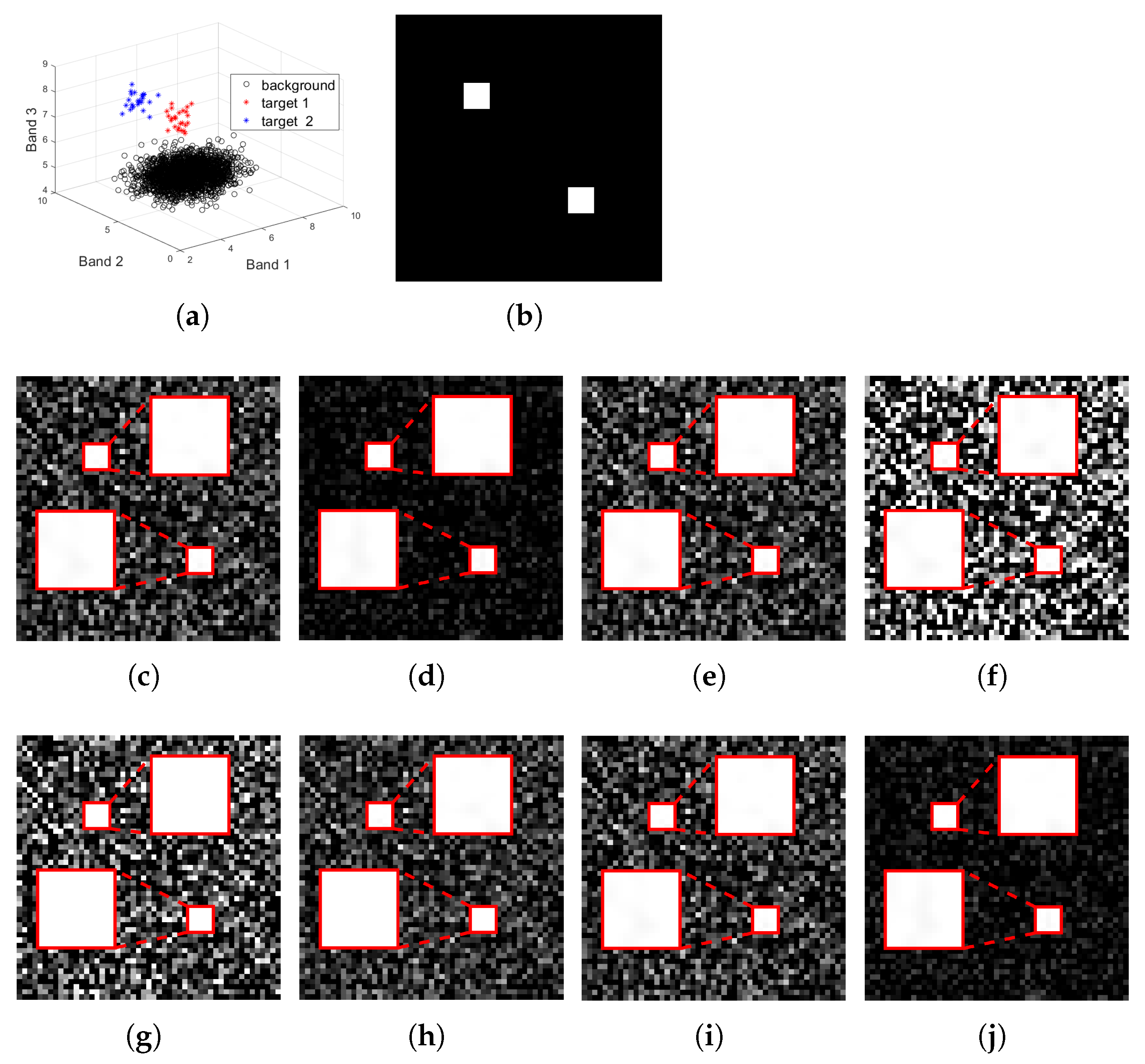
Target detection results for the simulated data with a size of 51 × 51 × 3 : (a): the distribution of the simulation image in three-dimensional spectral space, where the background pixels are marked in a black circle, and the targets are marked with red and blue asterisks; (b): the groundtruth image for the target d 1 = [ 5 , 5 , 7.5 ] T and d 2 = [ 4 , 6.5 , 8 ] T ; the detection result of (c) MTCEM where u = 0 , (d) MTMF where u = m , (e) MTR1 where u = r a n d ( 3 , 1 ) , and (f) MTR2 where u = r a n d ( 3 , 1 ) , (g) SCEM, (h) WTACEM, and (i) RMTCEM, respectively; (j): the detection result of MTCE ( u = u * ).
Remotesensing 17 02148 g001
Figure 2. 
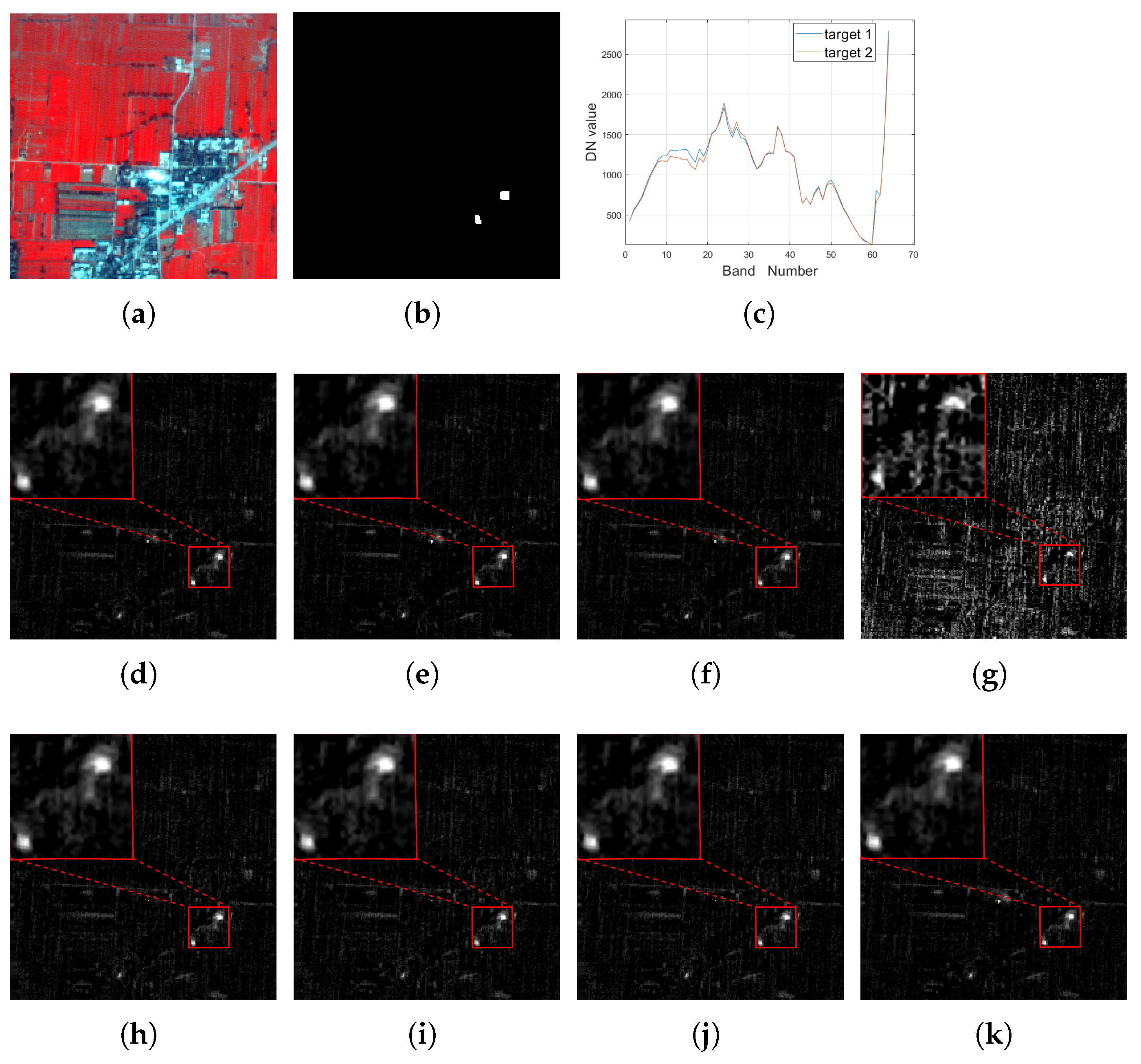
For the Xi’an data, (a): the false color image (R: 750.6 nm, G: 559.6 nm, B: 510.1 nm); (b) the groundtruth image for the target of interest; (c): the spectrum curve for the target of interest; the detection result of (d) MTCEM where u = 0 , (e) MTMF where u = m , (f) MTR1 where u = r a n d ( 3 , 1 ) , and (g) MTR2 where u = r a n d ( 3 , 1 ) using (h) SCEM, (i) WTACEM, and (j) RMTCEM, respectively. (k): The detection result of MTCE ( u = u * ).
Remotesensing 17 02148 g002
Figure 3. 
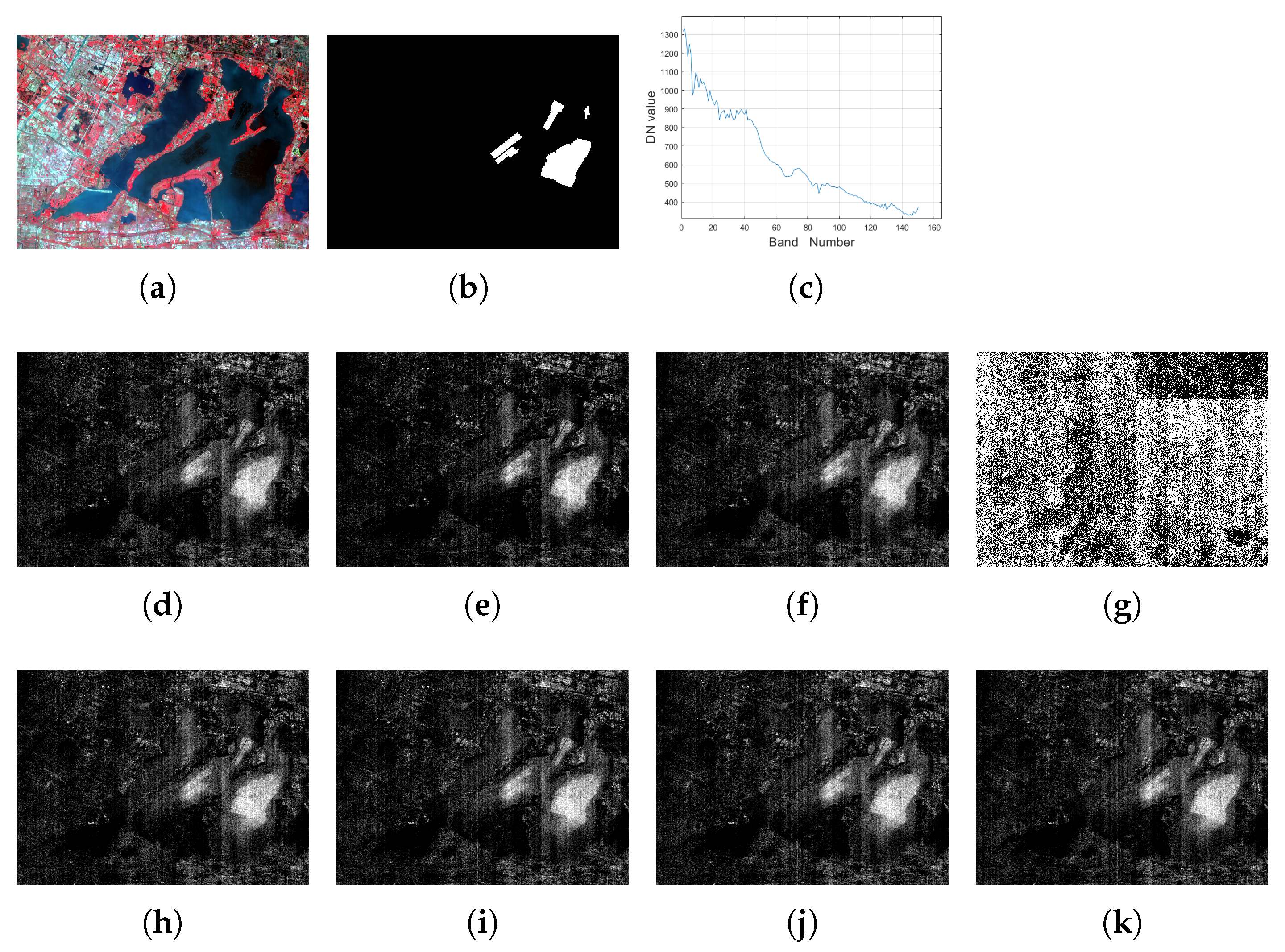
For the YCLake data, (a): the false color image (R: 860.88 nm, G: 651.31 nm, B: 548.66 nm); (b) the groundtruth image for the target of interest; (c): the spectrum curve for the target of interest; the detection result with p = 1 setting of (d) MTCEM where u = 0 , (e) MTMF where u = m , (f) MTR1 where u = r a n d ( 3 , 1 ) , and (g) MTR2 where u = r a n d ( 3 , 1 ) , (h) SCEM, (i) WTACEM, and (j) RMTCEM, respectively. (k): The detection result of MTCE ( u = u * ).
Remotesensing 17 02148 g003
Figure 4. Time consumption curve as a function of (a) the number of bands L; (b) the number of target p.
Remotesensing 17 02148 g004
Table 1. Notational conventions adopted in this article.
SymbolDescriptionSymbolDescription
LThe number of bandsNThe number of pixels
p 1 The number of selected target spectrum D p = [ d 1 , d 2 , , d p ] Target sample matrix
T Dataset m Mean vector of data T
R Correlation matrix of T K Covariance matrix of T
u Best data origin w u Projection detector varying with u
y Detection result output 1 p p-dimensional all-one vector
Table 2. Relation between the aforementioned algorithms and the generalized MTCE one.
Algorithm up Algorithm up
C E M 0 p = 1 M T C E M 0 p 1
M F m p = 1 M T M F m p 1
C E variable p = 1 M T C E variable p 1
Table 3. Computational complexity comparison of MTCE, MTCEM and MTMF, where L, N, p represents the number of the bands, total pixels, and target samples, respectively.
Algorithm Computational Complexity
M T C E O ( L 2 N + L 3 + 5 L 2 + 3 L 2 p + 3 L p 2 + 2 p 3 + 3 p 2 + 3 L p + 2 L + p + 2 L N ) .
M T C E M O ( L 2 N + L 3 + L 2 + L 2 p + L p 2 + p 3 + p 2 + L p + L N ) .
M T M F O ( L 2 N + L 3 + L 2 + L 2 p + L p 2 + p 3 + p 2 + 2 L p + 2 L N ) .
Table 4. Illustration of the confusion matrix of a binary classification.
TargetNon-Target
Hypothesized TargetTrue positive (TP)False positive (FP)
Hypothesized Non-targetFalse negative (FN)True negative (TN)
Table 5. Quantitative comparison of the average output energy (denoted E ) and four quantitative metrics, including AUC, OA, F-score (denoted ϝ ), and Kappa coefficient (denoted κ ), of different algorithms (including MTCEM, MTMF, MTR1, MTR2, and MTCE) for the simulated data. “-” means that their energy metric is not computed for a fair comparison. Bold numbers indicate the highest values in each row.
Metrics MTCEM MTMF MTR 1 MTR 2 SCEM WTACEM RMTCEM MTCE
E 0.12410.03850.12370.5414---0.0370
AUC 0.99660.99960.99660.86410.99870.99880.99660.9996
OA 0.96501.00000.98000.92100.98500.99500.97001.0000
ϝ 0.93461.00000.96150.92590.97030.99010.94341.0000
κ 0.91081.00000.94810.84200.96030.98680.92311.0000
Table 6. Quantitative comparison of the average output energy (denoted E ) and four quantitative metrics, including AUC, OA, F-score (denoted ϝ ), and Kappa coefficient (denoted κ ), of different algorithms (including MTCEM, MTMF, MTR1, MTR2, and MTCE) for the hyperspectral Xian data. “-” means that their energy metric is not computed for a fair comparison. Bold numbers indicate the highest values in each row.
Metrics MTCEM MTMF MTR 1 MTR 2 SCEM WTACEM RMTCEM MTCE
E ( × 10 3 ) 4.3874.2975.17768.7---4.278
AUC 0.95810.95940.95330.79670.94980.95190.95810.9594
OA 0.92760.92110.90460.75100.92430.91450.92430.9441
ϝ 0.86590.85540.82840.75110.85890.84340.86060.8931
κ 0.86590.85540.82840.50200.85890.84340.86060.8931
Table 7. The quantitative comparison of the average output energy (denoted E) and four quantitative metrics, including AUC, OA, F-score (denoted ϝ ), and Kappa coefficient (denoted κ ), of different algorithms (including MTCEM, MTMF, MTR1, MTR2, and MTCE) for the hyperspectral YCLake data. “-” means that their energy metric is not computed for a fair comparison. Bold numbers indicate the highest values in each row.
p Metrics MTCEM MTMF MTR 1 MTR 2 SCEM WTACEM RMTCEM MTCE
51 E 0.06890.07310.0689 6.1231 · 10 4 ---0.0681
AUC 0.98110.98240.98110.56360.98110.98110.98110.9824
OA 0.93820.93860.93980.52480.93850.93960.93720.9372
ϝ 0.88280.88410.88560.39070.88330.88520.88110.8817
κ 0.84100.84250.84490.07720.84170.84440.83860.8391
510 E 0.06380.06650.0638 6.4573 · 10 4 ---0.0623
AUC 0.95910.96280.95910.54580.96120.81330.95910.9628
OA 0.89430.90070.89300.50520.89660.73410.89250.9023
ϝ 0.80920.81890.80730.38510.81330.58740.80660.8212
κ 0.73700.75120.73430.06170.74270.40540.73320.7547
Table 8. Time consumption comparison of MTCEM, MTMF, SCEM, WTACEM, RMTCEM, and MTCE for the different datasets used in the subsections A, B, and C, where L, N, p represents the number of bands, pixels, and target samples, respectively.
DataLpNTime (s)
MTCEM MTMF SCEM WTACEM RMTCEM MTCE
sub . A 3226010.00080.00420.00510.00090.00990.0111
sub . B 64240,0000.00470.01190.01350.01180.04360.0456
sub . C 2001479,1440.18080.32080.20660.19200.50151.0526
sub . C 20010479,1440.15810.34540.57940.55722.15451.0881
Disclaimer/Publisher’s Note: The statements, opinions and data contained in all publications are solely those of the individual author(s) and contributor(s) and not of MDPI and/or the editor(s). MDPI and/or the editor(s) disclaim responsibility for any injury to people or property resulting from any ideas, methods, instructions or products referred to in the content.

