Automatic Detection of Landslide Surface Cracks from UAV Images Using Improved U-Network

Abstract

Surface cracks are key indicators of landslide deformation, crucial for early landslide identification and deformation pattern analysis. However, due to the complex terrain and landslide extent, manual surveys or traditional digital image processing often face challenges with efficiency, precision, and interference susceptibility in detecting these cracks. Therefore, this study proposes a comprehensive automated pipeline to enhance the efficiency and accuracy of landslide surface crack detection. First, high-resolution images of landslide areas are collected using unmanned aerial vehicles (UAVs) to generate a digital orthophoto map (DOM). Subsequently, building upon the U-Net architecture, an improved encoder–decoder semantic segmentation network (IEDSSNet) was proposed to segment surface cracks from the images with complex backgrounds. The model enhances the extraction of crack features by integrating residual blocks and attention mechanisms within the encoder. Additionally, it incorporates multi-scale skip connections and channel-wise cross attention modules in the decoder to improve feature reconstruction capabilities. Finally, post-processing techniques such as morphological operations and dimension measurements were applied to crack masks to generate crack inventories. The proposed method was validated using data from the Heifangtai loess landslide in Gansu Province. Results demonstrate its superiority over current state-of-the-art semantic segmentation networks and open-source crack detection networks, achieving F1 scores and IOU of 82.11% and 69.65%, respectively—representing improvements of 3.31% and 4.63% over the baseline U-Net model. Furthermore, it maintained optimal performance with demonstrated generalization capability under varying illumination conditions. In this area, a total of 1658 surface cracks were detected and cataloged, achieving an accuracy of 85.22%. The method proposed in this study demonstrates strong performance in detecting surface cracks in landslide areas, providing essential data for landslide monitoring, early warning systems, and mitigation strategies.

1. Introduction

Landslides are common natural disasters, often causing significant loss of life and property, especially when they occur near residential areas or infrastructure. Anticipated climate and environmental changes are expected to increase the risk of landslides [1]. Prompt identification and continuous monitoring are critical for mitigating landslide hazards. Surface cracks frequently appear in landslide areas due to factors like uneven internal stress of slope materials, rising groundwater levels, rainfall, and earthquakes. These cracks can exacerbate the influence of external triggers on slopes, leading to progressive deformation or even instability of the landslide mass. As a primary macroscopic indicator of landslide deformation, the timely detection and delineation of surface cracks contribute to landslide identification and understanding their deformation characteristics. Recognizing these surface features facilitates early detection of potential failure precursors, enabling preventive measures to reduce losses. Moreover, analyzing crack locations and patterns aids in deciphering landslide deformation trends, guiding the deployment of field monitoring instrumentation [2,3].

Landslide areas are typically characterized by complex terrain and varying sizes, rendering manual crack detection both challenging and inefficient. Unmanned aerial vehicle (UAV) technology offers a solution due to its flexibility, cost-effectiveness, and capability to acquire high spatial resolution imagery. Equipped with RGB cameras, UAVs capture photographs that can be processed using photogrammetric techniques to generate high-resolution digital orthophoto maps (DOMs). These DOMs provide detailed representations of crack textures, shadows, and morphological shapes, enabling manual visual interpretation or facilitating fully/semi-automated crack detection through digital image processing and machine learning algorithms. For instance, Wang et al. [4] employed Otsu thresholding and the Canny edge detector to identify cracks on landslide rear edges. Al-Rawabdeh et al. [5] extracted landslide scarp features using 3D point cloud data generated from high-resolution UAV imagery, calculating slope and terrain roughness indices. Similarly, Deng et al. [6] utilized point cloud and DOM data, leveraging features like point cloud roughness, slope, and dispersion for crack detection. Their subsequent research [7] further advanced detection accuracy through a multi-dimensional information fusion method. These methods are generally straightforward and do not require pretraining datasets. However, achieving accurate crack detection with these methods relies heavily on selecting appropriate segmentation thresholds, a process significantly hindered by complex backgrounds or varying lighting conditions.

Significant advancements in image processing have occurred in recent years, primarily driven by the rapid development of deep learning, particularly convolutional neural networks (CNNs). This progress has prompted extensive exploration of CNNs for crack detection, typically framed as either semantic segmentation or object detection tasks. Semantic segmentation, unlike object detection, provides pixel-level classification maps highly beneficial for both qualitative assessment and quantitative analysis of cracks. Consequently, this study approaches crack detection as a semantic segmentation task. Numerous studies have demonstrated the effectiveness of CNNs for crack detection. However, the predominant focus has been on detecting cracks on various anthropogenic structures, such as bridges [8,9], roads [10,11,12], walls [13], buildings [14], and other civil infrastructure [15]. Subsequent quantification of crack characteristics (e.g., length, width, density, topology) is often meticulously performed to assess the extent of structural damage [16].

Detecting cracks on the intricate and irregular surfaces of landslide regions presents distinct challenges compared to smoother, more uniform artificial surfaces. While some efforts have focused on detecting natural surface cracks, the supporting data predominantly originate from laboratory settings or ground-based photography [17,18]. This data collection paradigm, however, is unsuitable for the large-scale, area-wide image acquisition required in expansive landslide terrains. Recent studies address this using UAV imagery: Yu et al. [19] developed a deformable convolution network for earthquake-induced cracks, Tao et al. [20] applied deep residual shrinkage U-Net in mining regions, Sandric et al. [21] implemented U-Net and DeepLab for landslide cracks, and Cheng et al. [22] used RetinaNet for landslide crack identification. These studies highlight considerable potential; nonetheless, to our knowledge, current research remains predominantly focused on model development, with integrated detection-to-cataloging workflows requiring further development.

Advanced semantic segmentation models, including U-Net [23], PSPNet [24], DeepLabv3+ [25], and UCTransNet [26], have demonstrated outstanding performance in segmentation tasks. Among these, U-Net’s architecture offers simplicity, ease of implementation, and high performance with limited training data [27], making it suitable for landslide crack datasets. However, two challenges persist: (1) complex background noise (e.g., vegetation, gravel, shadows) obscuring crack features, reducing feature extraction efficacy; and (2) information loss during pooling or downsampling, causing encoder–decoder semantic discrepancies.

To address these challenges, this study establishes a comprehensive automated pipeline for landslide crack detection and cataloging. Specifically, high-resolution landslide imagery is first acquired using UAVs, providing fundamental data for crack detection. Subsequently, an improved encoder–decoder semantic segmentation network (IEDSSNet) is proposed based on the U-Net architecture to enhance feature extraction and reconstruction capabilities, thereby improving segmentation accuracy in complex surface environments. Furthermore, morphological operations combined with connected-component analysis are applied for post-processing segmentation results, enhancing output robustness. Finally, crack lengths and widths are quantitatively measured from the segmented results, followed by instance-level cataloging to enhance the utility of detection results. The proposed pipeline was applied to the Heifangtai landslide area in Gansu Province, China, generating an accurate regional inventory of surface cracks. The accuracy and effectiveness of the results were evaluated through visual interpretation.

2. Methodology

This section first presents an overview of the crack detection pipeline. Then, we detail the IEDSSNet and all its components, including the enhanced encoder and decoder, as well as the loss function employed. Finally, methods for post-processing and measuring crack lengths and widths are provided.

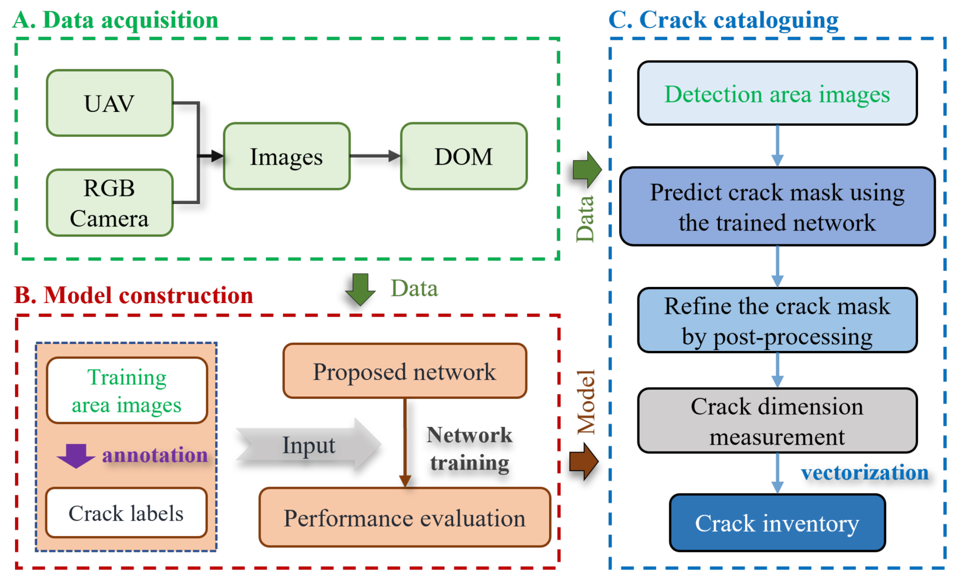
2.1. Pipeline of Landslide Surface Crack Detection

Figure 1 illustrates the automated workflow for landslide surface crack detection in UAV imagery. The procedure comprises three stages: (1) data acquisition, (2) model construction, and (3) crack cataloging.

The initial stage involves UAV-based data acquisition, photogrammetric processing, and DOM generation. Low-altitude UAV flights provide superior spatial resolution compared to satellite imagery, enabling detailed observation of landslide surface cracks. This stage requires three main steps: planning UAV flight paths over the target area, executing image acquisition missions, and processing collected imagery through structure-from-motion (SfM) photogrammetry to generate DOMs.

The next stage involves developing a crack segmentation model, termed IEDSSNet, as outlined in Section 2.2. Constructing this model entails designing its architecture and training its weight parameters using input data. These input data include images of cracks paired with their corresponding labels, composed of both DOM data and manually annotated labels.

The final cataloging stage processes UAV imagery using the trained model. First, the model generates crack probability masks for the target region. To address noise and discontinuities inherent in complex terrain, post-processing techniques including morphological operations and connected-component analysis are applied to refine these predictions. Finally, each crack is vectorized, and its width and length, measured based on DOM resolution, are recorded in the vector attributes, completing the crack inventory. For details on post-processing and measurements, see Section 2.3.

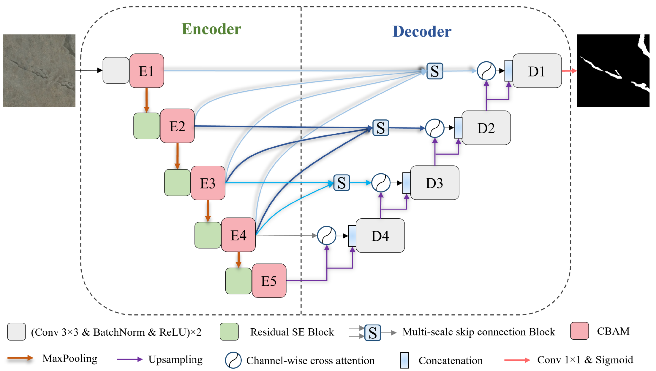
2.2. Proposed Crack Segmentation Network Architecture

As Figure 2 illustrates, the structure of the proposed IEDSSNet is similar to U-Net, as both adopt an encoder–decoder architecture. To enhance the network’s ability to extract effective crack features in complex backgrounds, we integrated residual squeeze-and-excitation (SE) blocks and convolutional block attention module (CBAM) blocks into the encoder. Additionally, to narrow the semantic gap between encoder and decoder features, traditional skip connection blocks were replaced with multi-scale skip connection blocks, and channel-wise cross attention blocks were incorporated into the decoder. Specific details were introduced in Section 2.2.1 and Section 2.2.2.

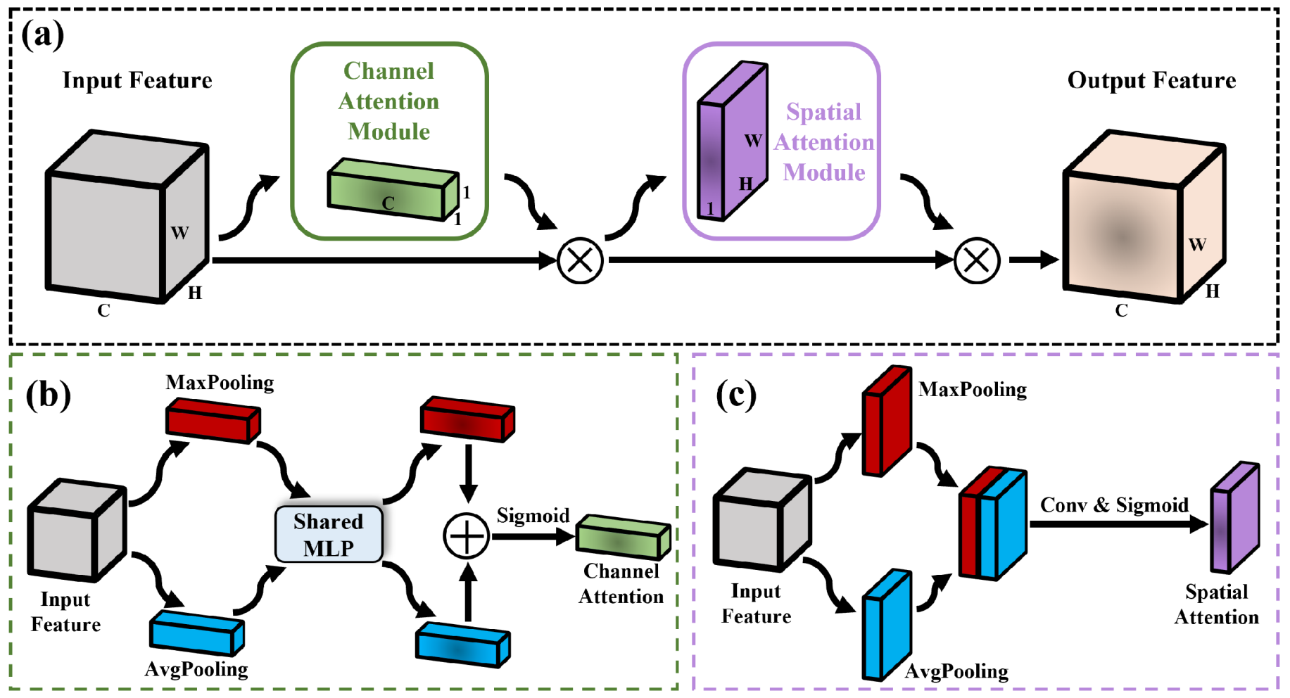
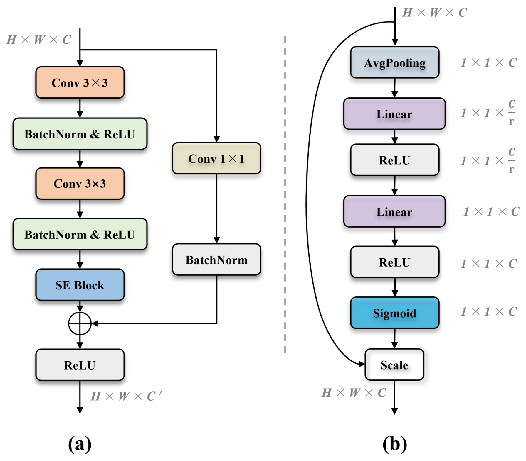
2.2.1. Enhanced Feature Extraction Encoder

The CBAM block, known for its simplicity and efficacy as an attention mechanism, dynamically refines feature maps [28]. Its structure, depicted in Figure 3, comprises channel and spatial attention components. For a feature map with dimensions (H,W,C), channel attention applies max-pooling and average-pooling along channel dimensions, producing feature maps of size (1,1,C). These undergo processing through a shared MLP module (convolution and ReLU activation) followed by sigmoid mapping, yielding channel attention weights. Spatial attention operates similarly on spatial dimensions. While channel attention highlights crack-relevant channels, spatial attention focuses on crack locations. Pooling operations in the encoder cause spatial information loss that particularly harms small targets like cracks. Therefore, we deploy CBAM blocks before pooling and downsampling to refine multi-scale feature, mitigating crack information loss and enhancing feature representational capability.

The residual SE block combines the SE attention mechanism with the residual block, as illustrated in Figure 4. Initially, two 3 × 3 convolution operations with BatchNorm and ReLU activation extract semantic features from the input feature map. Subsequently, the SE block enhances the input feature map, while simultaneously, the original feature map undergoes a 1 × 1 convolution and BatchNorm operation. The final output feature map is obtained by adding the two feature maps and applying ReLU activation. This standard residual block facilitates direct gradient flow through the shorter path, alleviating the vanishing gradient issue during training [29].

It is important to note that we have integrated the SE block into the residual block, as shown in Figure 4b. First, it performs global average pooling on the feature map, compressing it to the channel dimension. Subsequently, the significance of each channel is learned through two fully connected layers. The first layer reduces the channel dimension by a factor of r, while the second layer restores it. Finally, channel importance weights are determined using a sigmoid function, enhancing important features and suppressing irrelevant ones. This approach improves model accuracy by learning the importance of different channels while preserving the original features. Residual blocks are effective for handling deeper networks, and the SE block further emphasizes critical features. Together, they capture more complex or detailed features while mitigating gradient vanishing, improving the extraction of semantic crack features.

As depicted in Figure 2, the enhanced encoder comprises convolutional layers, max-pooling layers, residual SE blocks, and CBAM blocks, aimed at extracting semantic features from input RGB images. The encoder processes images with dimensions (H,W,3), where H and W denote the height and width, respectively. It is structured into five stages, each corresponding to different scales of semantic features. In the first stage, the input image undergoes feature extraction via two sets of 3 × 3 convolutions, followed by BatchNorm and ReLU activation. The CBAM block refines these features into the first-scale semantic feature, E1, with 64 channels and unchanged spatial dimensions. Subsequently, in the second stage, the feature map size is halved through max-pooling, with further enhancement via a residual SE block and a CBAM block, resulting in the second-scale semantic feature, E2, sized $({\displaystyle \frac{H}{2}},{\displaystyle \frac{W}{2}},128)$. The subsequent three stages employ a similar process, starting with max-pooling to reduce feature map size, followed by feature extraction using a residual SE block and a CBAM block. With decreasing spatial dimensions, the convolutional layers in each stage capture more extensive image context information, generating increasingly complex and abstract features. Notably, the residual SE block is omitted in the first stage to retain more low-level features for subsequent feature extraction. Features E3, E4, and E5 correspond to ${\displaystyle \frac{1}{4}}$,${\displaystyle \frac{1}{8}}$, and ${\displaystyle \frac{1}{16}}$ of the input image size, with channel depths of 256, 512, and 512, respectively. The absence of doubled channel numbers in the fifth stage helps control the model’s parameter count.

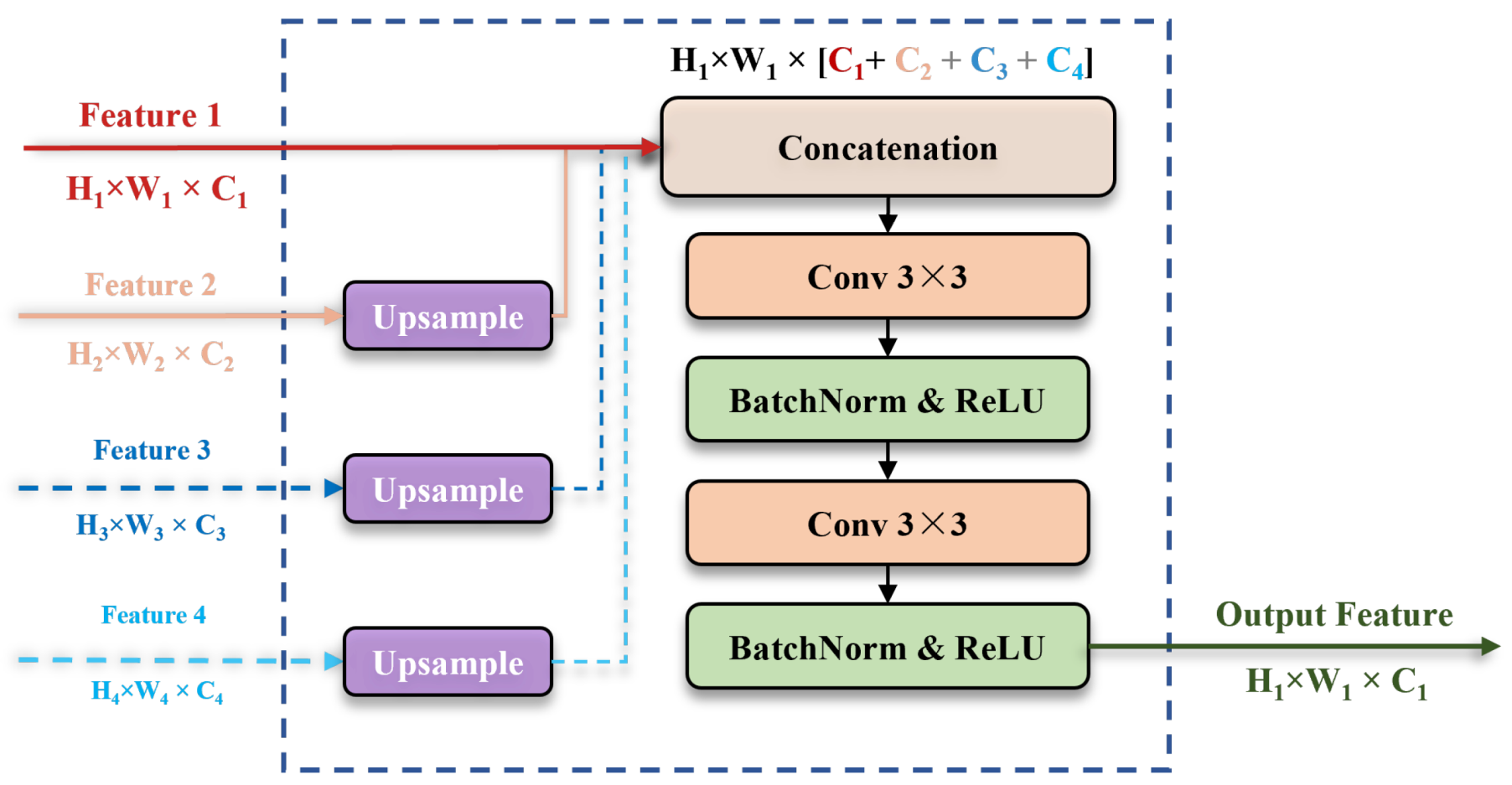
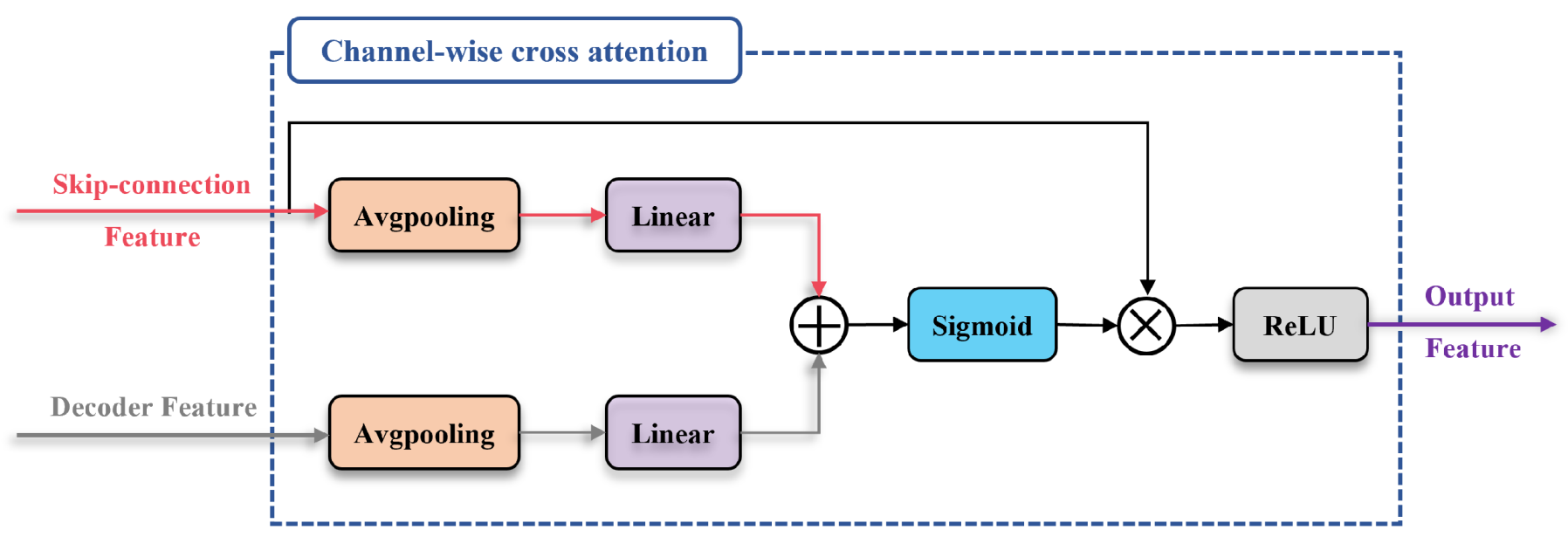
2.2.2. Enhanced Feature Reconstruction Decoder

The conventional U-Net utilizes convolutional and pooling operations to extract higher-level abstract features, progressively compressing the input image. However, this process may lead to the loss of detailed information. On the contrary, the decoder’s objective is to reconstruct these abstract features and map them back to the original image space. Nonetheless, a semantic gap arises between the encoder and decoder due to information loss and reduced resolution caused by pooling operations [30]. While skip connections partially alleviate this semantic gap by utilizing feature information from the corresponding encoder’s single scale, to fully leverage feature information across different scales, we introduced a multi-scale skip connection block as illustrated in Figure 5.

The new skip connection block can accept 2 to 4 features as input, leading to enhanced feature representation. Within our network, we designate the low-scale feature (Feature 1) as the reference. By aligning the spatial dimensions of other input features to it and concatenating the feature maps along the channel dimension, we generate a multi-scale feature with spatial dimensions of $H_1\times W_1$ and a maximum channel depth of $C_1$ + $C_2$ + $C_3$ + $C_4$. Subsequently, through two convolutional operations, BatchNorm, and ReLU activation, we adjust the channel depth to match the reference feature $C_1$. The skip connection approach integrates both shallow and deep abstract features, facilitating simultaneous consideration of local details and broader contextual information. This strategy helps narrow semantic gap between encoder and decoder features.

Additionally, we integrated a channel-wise cross attention block into the decoder to fuse multi-scale skip connection features with decoder features, further reducing semantic-level inconsistencies [26]. As shown in Figure 6, this block takes the fused features from multi-scale skip connections and corresponding features from the decoder stage as input, producing fused features as output. Initially, input features undergo spatial compression through global average pooling, reducing feature map dimensions to (1,1,C). These features are then nonlinearly transformed into channel attention via a linear layer. Subsequently, the channel attention of both features is fused through addition, and a sigmoid activation function is used to map the fused attention to attention weights. Finally, the input skip connection features are multiplied by attention weights and passed through a ReLU activation function to generate the output features. The channel-wise cross attention block is based on decoder features to guide channel and information filtering of multi-scale skip connection features, thereby reducing ambiguity between the skip connection features and decoder features.

Aligned with the encoder, the decoder is organized into five stages, with feature dimensions at each stage matching those of the corresponding encoder stage. Its purpose is to gradually restore the abstract semantic features within the decoder to the dimensions of the input image. In the fifth stage of the decoder, features from the fifth encoder stage are upsampled and input into channel-wise cross attention along with features E4 from the fourth encoder stage, resulting in output features. These output features are then concatenated with upsampled features E5 and processed through two convolutional layers followed by ReLU activation to generate the decoder features D4. The subsequent three stages are similar to the fifth stage, but the encoder features fuse features from multiple scales, as illustrated in Figure 5. Finally, the first decoder stage maps the feature map to a predictive probability map using a 1 × 1 convolutional layer and sigmoid activation function. In this study, a threshold of 0.5 is used to distinguish between crack targets and background.

2.2.3. Loss Function

We combine binary cross entropy (BCE) loss and dice loss to evaluate the prediction error of segmentation outcomes, as defined in Equation (1). The formula consists of two parts: the first part represents the BCE loss, which emphasizes the accuracy of pixel-level predictions. The second part represents the dice loss, which prioritizes region-level overlap and is particularly suitable for managing class imbalance and enhancing the network model’s attention to boundaries [31].

$$L(y,\widehat{p})=-\left[ylog\widehat{p}+(1-y)log(1-\widehat{p})\right]+{\displaystyle \frac{y+\widehat{p}-2y\widehat{p}}{y+\widehat{p}+1}}$$

(1)

where $\widehat{p}$ represents the estimated probability of the network model’s prediction, and y denotes the ground truth.

2.3. Crack Mask Post-Processing and Cataloging

The IEDSSNet we proposed accurately segments landslide surface cracks, enabling the prediction of crack masks for areas of interest. However, due to the complexity of surface backgrounds and limitations in the model’s predictive accuracy, the predicted crack mask may inevitably contain incomplete or false positive noise cracks. Therefore, further post-processing of the crack mask is necessary to enhance the robustness of crack segmentation results. Additionally, to enhance the practical utility of the crack segmentation mask, we quantify the length and width of the cracks, then vectorize them into an instance-level crack inventory.

First, morphological closing operations are applied to refine the predicted crack mask. Morphological closing involves two operations: dilation and erosion, as shown in Equation (2). Through morphological closing, small holes in the crack mask are eliminated, small fractures are connected, and the boundaries of cracks are smoothed.

$$\mathrm{Closing}(C,K)=(C\ominus K)\oplus K$$

(2)

where C represents the crack mask, K represents the structural element, ⊖ denotes the erosion operation, used to shrink the mathematical morphology of crack boundary pixels, and ⊕ denotes the dilation operation, which expands the mathematical morphology of crack boundary pixels.

Although morphological closing can optimize the crack mask to some extent, it may incorrectly label pixels similar to cracks as cracks, particularly in complex ground backgrounds, leading to isolated pixel clusters. Given that cracks typically exhibit elongated characteristics, this study proposes a connected-component filtering method to eliminate false positives. A connected component is retained as a potential crack if it satisfies either of the following conditions: the aspect ratio of its minimum bounding rectangle exceeds a predefined threshold, or the area ratio (connected-component area to bounding rectangle area) falls below a specified value (preserving curved cracks). This approach leverages geometric properties to distinguish true cracks from noise while preserving detection completeness.

After obtaining the refined crack segmentation mask, we measure the width and length of each crack at the pixel scale using digital image processing techniques. First, we derive a skeleton representing the crack’s shape using the medial axis transform (MAT) proposed by Blum et al. [32]. MAT helps assess the significance of terminal branches and identify local boundary points. However, due to jagged crack boundaries in images, the MAT skeleton may include false branches, affecting the accuracy of crack measurements. To address this, we apply the discrete skeleton evolution (DSE) method developed by Bai et al. [33] to remove false branches. As shown in Figure 7b, red pixels depict the crack skeleton, while white pixels are false branches removed by the DSE. We record the length of the red pixels as the crack length at the pixel scale.

Due to the uncertainty in measuring the width at crack bifurcations, we exclude crack pixels within the maximum inscribed circle centered at the skeleton bifurcations. Figure 7c shows the crack edges and skeleton after removing intersecting regions. We use a hybrid method by Ong et al. [34] for width measurement. This method combines shortest projection and orthogonal to identify point pairs achieving the shortest distance orthogonal to the skeleton. The green lines in Figure 7d represent multiple width measurements obtained by this method. We average these green lines to determine the crack width. After measuring the length and width of all cracks, we convert them to real distances by multiplying them with the DOM spatial resolution. Finally, using the rasterio library in the Python 3.8.5 environment, we convert the crack mask into polygon vectors and add the measured crack length and width as attributes to the vectors. The resulting crack inventory aids in data visualization, management, and decision-making for prevention and control.

3. Experiments and Results

The study area and the constructed dataset are detailed in Section 3.1. The evaluation metrics and specific experimental settings for the model are outlined in Section 3.2. Section 3.3 presents the performance results of crack segmentation using the network model. Finally, Section 3.4 details the results of cataloging landslide surface cracks.

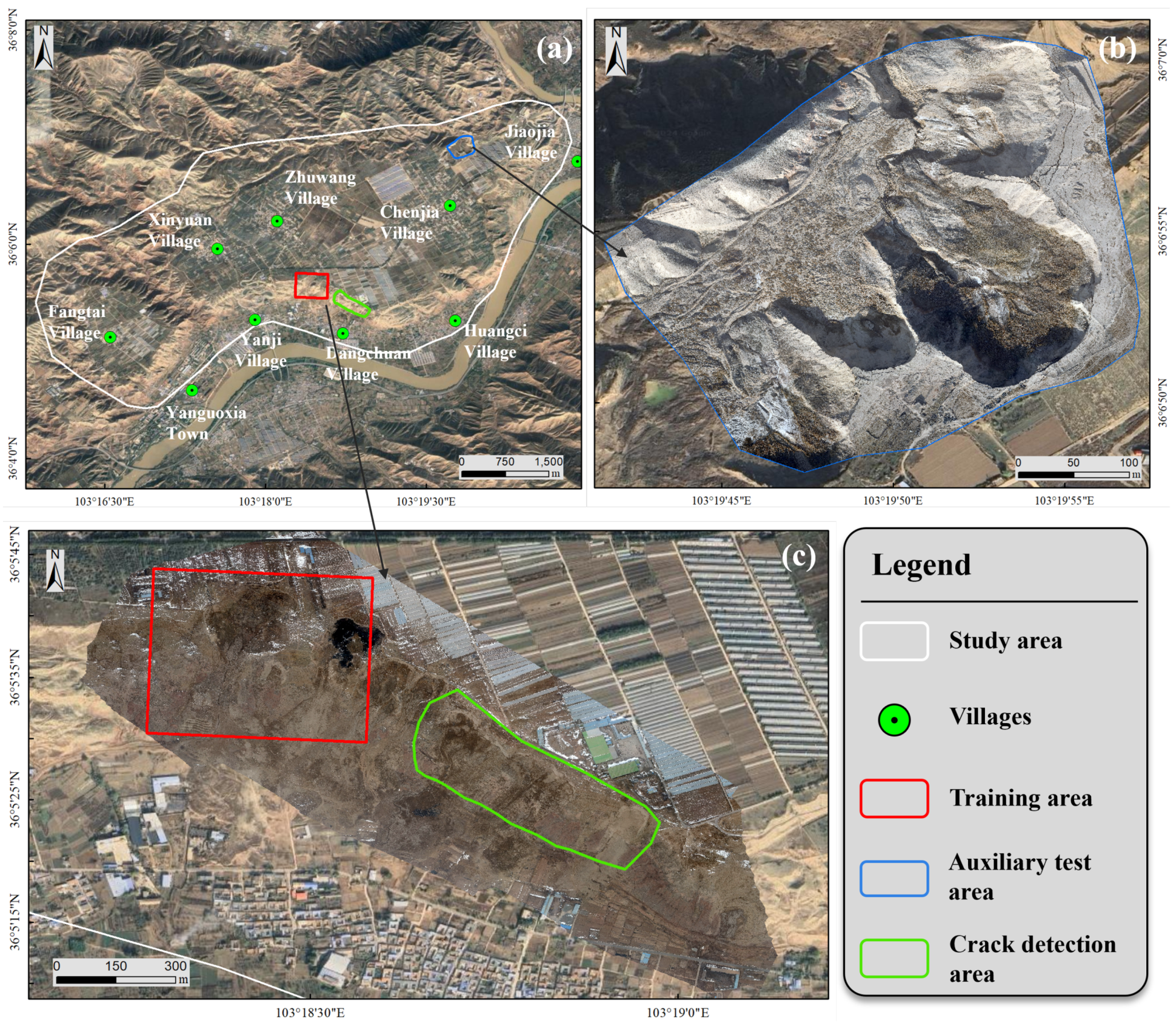
3.1. Study Area and Dataset Preparation

The study area is situated on the northern bank of the Yellow River, in Yanguoxia Town, Yongjing County, Linxia Hui Autonomous Prefecture, Gansu Province, China. The area experienced a typical loess flow slide event on 27 January 2021 [35], delineated by the green boundary in Figure 8. Fortunately, Chang’an University issued a timely cautionary alert seven hours prior to the landslide incident, mitigating potential casualties effectively [36]. However, the unstable slope after the landslide continues to threaten residents’ lives and properties, necessitating ongoing monitoring of crack distribution in the area. Therefore, this study designates the area as the crack detection area, selecting a specific region on the northwest side for training and testing the proposed IEDSSNet, as indicated by the red border in Figure 8. On 15 February 2023, we conducted aerial imaging of the study area using the DJI M300 RTK UAV equipped with a Zenmuse P1 full-frame camera. Flight operations were conducted at 150 m above ground level with 80% heading overlap and 70% side overlap. Further details can be found in our previous work [2]. A total of 806 clear and complete images were captured. The images were then processed using DJI Terra software 3.6.6 for two-dimensional visible light reconstruction, resulting in a DOM with a spatial resolution of 2 cm, as shown in Figure 8c.

Firstly, we cropped the DOM images of the training area, sized at 22,672 × 17,391 pixels. Due to GPU limitations, we used a sliding window approach to crop the images into 256 × 256 pixel segments. We then meticulously annotated the cracks in the images using the open-source Labelme tool, resulting in a dataset of 240 surface crack images with corresponding labels. We randomly divided the dataset into a training set and a validation set in a 4:1 ratio, with the training set containing 192 images and the validation set containing 48 images. Given the inadequacy of the 192 images for robust model training, we augmented the dataset by applying horizontal and vertical flipping and rotation to increase sample diversity. This resulted in a total of 1152 training images with diverse characteristics. The augmented data were used for model training, while the validation dataset was used to evaluate the model’s performance. Examples of crack images and their labels are shown in Figure 9.

Considering that a limited training sample set was used for model development, while generalization capability is critical for practical crack detection, we introduced an auxiliary test area (blue-bordered region in Figure 8b) for performance evaluation. This area contains naturally distributed cracks resulting from historical landslide events. The DOM was acquired on 31 December 2023 under significantly different illumination conditions compared to the training region, despite similar loess lithology. Such variations permit partial assessment of generalizability for optical image-based detection models. The DOM was also cropped into 256 × 256 pixel segments with meticulous manual annotation, generating an auxiliary test dataset of 111 samples. The summary of the study dataset is shown in

Table 1. Summary of the study dataset.

Dataset	Samples	Source	Augmentation	Resolution
Training set	1152	Training area	Yes	2 cm/pixel
Primary test set	48	Training area	No	2 cm/pixel
Auxiliary test set	111	Auxiliary test area	No	1.5 cm/pixel

.

3.2. Evaluation Metrics and Experimental Settings

We quantitatively evaluate the model’s performance using commonly used semantic segmentation tasks: intersection over union (IOU), recall, precision, and F1 score. IOU measures the overlap between the model’s predicted crack areas and the actual crack areas. Recall denotes the ratio of correctly predicted crack pixels to the actual crack pixels, reflecting the model’s crack identification ability. Precision represents the proportion of correctly predicted crack pixels to all pixels predicted as crack pixels, indicating the model’s precision in predicting cracks. The F1 score, a harmonic mean of recall and precision, provides a balanced assessment of the model’s precision and completeness. It is worth noting that, due to sample imbalance in crack segmentation, the study did not use the accuracy metric to avoid potentially misleading results. The specific formulas for these metrics are as follows:

$$IOU={\displaystyle \frac{TP}{TP+FP+FN}}$$

(3)

$$Recall={\displaystyle \frac{TP}{TP+FN}}$$

(4)

$$Precision={\displaystyle \frac{TP}{TP+FP}}$$

(5)

$$F_{1}score={\displaystyle \frac{2\times Precision\times Recall}{Precision+Recall}}$$

(6)

where $TP$ (true positive) represents pixels correctly predicted as cracks, $FP$ (false positive) represents pixels incorrectly identified as cracks, and $FN$ (false negative) represents pixels incorrectly predicted as background.

Furthermore, it is essential to evaluate the complexity of models to understand the performance and resource utilization in practical applications. Typically, the complexity of network models is analyzed from two perspectives: space and time. The number of parameters (Params) and floating-point operations (FLOPs) are the two most widely used metrics for measuring the spatial and temporal complexity of a model, respectively; their units are mega (M) and giga (G), where smaller values indicate lower corresponding complexities. For example, considering a standard convolution with bias, the corresponding number of parameters and FLOPs are shown in Equations (7) and (8).

$$Params=(K_w\times K_h\times C_{in})\times C_{out}+C_{out}$$

(7)

$$FLOPs=Params\times W_{out}\times H_{out}$$

(8)

where $K_w$ and $K_h$ denote the width and height of the convolution kernel, $C_{in}$ and $C_{out}$ represent the number of input channels and output channels, respectively, and $W_{out}$ and $H_{out}$ indicate the width and height of the output feature map.

In this study, all network models were implemented using PyTorch 1.13.1 and CUDA 11.7 libraries within the python environment. Training took place on the Chang’an University high-performance computing platform, equipped with multiple Nvidia A800-80 G GPUs, although only a single GPU was used for training in this study. A total of 150 training epochs were conducted. The initial learning rate was set to $5\times {10}^{-5}$. For the first four epochs, it was warmed up to 10 times the initial learning rate, then gradually decreased to $5\times {10}^{-6}$ using the cosine annealing method. Learning rate warm-up enhances stability in the initial training stages [37], while cosine annealing reduces and restarts the learning rate during training to avoid false local minima [38]. Model parameter updates were carried out using the Adam optimizer [39]. Finally, training used mini-batches of size 4, incorporating random adjustments to the hue, saturation, and brightness of images during data loading, thus exposing the model to a rich variety of sample combinations and enhancing its robustness. It should be noted that, following prior research in crack detection [10,19], all methods were trained from scratch without pretrained models, primarily considering three aspects: (1) significant semantic discrepancies between existing datasets (e.g., PASCAL VOC2012 [40], MS-COCO [41]) and the landslide crack domain, (2) the comparative simplicity of crack segmentation as a two-class problem, and (3) the contribution of the aforementioned training strategies to model convergence during training.

3.3. Crack Segmentation Performance Analysis

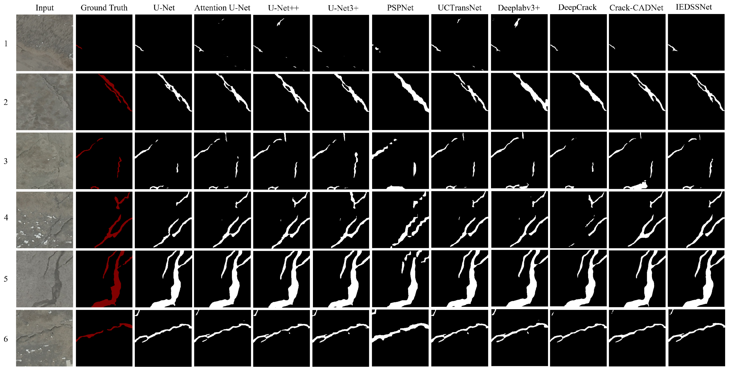
3.3.1. Comparison Between IEDSSNet and Other Methods

To assess the crack segmentation performance of IEDSSNet, we conducted a comparative analysis against recent generic semantic segmentation methods, including U-Net [23], Attention U-Net [42], U-Net++ [43], U-Net3+ [44], PSPNet [24], UCTransNet [26], and Deeplabv3+ [25]. Additionally, we compared our method with two open-source neural network models designed specifically for crack detection, namely DeepCrack [10] and Crack-CADNet [19]. These methods are widely recognized in the fields of semantic segmentation and crack detection. Attention U-Net extends U-Net by integrating an attention mechanism to enhance the model’s focus on regions of interest. U-Net++ and U-Net3+ introduce nested or multi-scale skip connections. PSPNet leverages pyramid pooling modules to augment receptive fields and achieve multi-scale feature fusion through spatial pyramid pooling. UCTransNet introduces transformer architecture for semantic segmentation, facilitating the capture of long-range dependencies within images via self-attention mechanisms. Deeplabv3+ represents an advancement within the Deeplab series, enhancing semantic segmentation precision and robustness through spatial pyramid pooling and decoder modules. DeepCrack learns multi-scale deep convolutional features through hierarchical convolution stages and then integrates them to capture the linear structures of cracks. Crack-CADNet is a network architecture designed for seismic crack detection. It utilizes adaptive deformable convolutions to handle the spatial characteristics of the sinuous linear cracks.

Table 2. Performance of different models in primary test set.

Network	IOU (%)	Recall (%)	Precision (%)	F1 Score (%)	Params (M)	FLOPs (G)
U-Net	65.02	76.53	81.20	78.80	31.03	54.65
Attention U-Net	66.10	77.10	82.24	79.59	34.88	66.57
U-Net++	64.47	75.93	81.03	78.40	36.63	138.60
U-Net3+	65.36	78.84	79.27	79.06	16.35	170.95
PSPNet	53.74	73.28	66.84	69.91	46.58	25.89
UCTransNet	65.43	77.03	81.29	79.10	78.83	36.23
Deeplabv3+	64.98	80.49	77.13	78.77	59.34	22.24
DeepCrack	60.78	70.29	81.79	75.61	30.91	137.06
Crack-CADNet	66.23	77.95	81.51	79.69	20.17	15.38
IEDSSNet	69.65	80.77	83.49	82.11	18.82	99.20

lists the evaluation results of IEDSSNet and nine comparative methods on the primary test set. The IEDSSNet outperformed all others across all metrics, achieving an F1 score of 82.11% and an IOU of 69.65%. In comparison with the second-best model, Crack-CADNet, the IEDSSNet exceeded it by 3.42% and 2.42% in terms of IOU and F1 score, respectively. PSPNet exhibited the poorest performance, achieving IOU and F1 scores of only 53.74% and 69.91%, respectively. A trade-off exists between recall and precision; while high recall suggests the model can identify most true cracks, it may lead to more false positives, whereas high precision indicates the model can identify most true cracks but may result in more false negatives. Among the seven comparison methods, Deeplabv3+ achieved the highest recall of 80.49%, while its precision was 77.13%. In contrast, the model with the highest precision was Attention U-Net, reaching 82.24%, but its recall was only 77.10%. Overall, our proposed IEDSSNet maintained high recall and precision simultaneously, achieving 80.77% and 83.49%, respectively.

From Table 2, it can be seen that different models have varying time and space complexities. The parameter count of IEDSSNet (18.82 M) is second only to UNet3+ (16.35 M), belonging to models with smaller network architectures. However, its FLOPs (99.20 G) are relatively high, although lower than U-Net++ (138.60 G), U-Net3+ (170.95 G), and DeepCrack (137.06 G). For the task of detecting surface cracks in landslide areas, we can accept achieving better detection performance at the cost of some inference time. Furthermore, considering the continually advancing modern GPU hardware, the complexity of the IEDSSNet is quite acceptable.

Figure 9 displays partial crack sample images alongside the prediction results from different methods. These samples encompass both small cracks, like samples 1 and 3, and wider cracks, such as samples 4, 5, and 6; some backgrounds are relatively simple, like samples 2, 3, and 5; while others feature more complex backgrounds abundant with grass and snow, like samples 1, 4, and 6. Visually, PSPNet exhibits the poorest prediction performance, merely segmenting the approximate crack positions with minimal crack edge details. Each model performs relatively well in segmenting both small and wide cracks. However, in scenarios with more complex background interference, the IEDSSNet effectively filters out background information erroneously identified as cracks by other comparative methods, thus preserving the most detailed crack information. For example, in samples 1 and 4, besides the PSPNet network model with low attention to crack details, the other eight comparative methods incorrectly segment some grass shadows or snow edges as crack pixels. Two open-source networks for crack detection also performed slightly worse than IEDSSNet. For instance, the DeepCrack network exhibited significant missing parts in its predictions for samples 3 and 4, while Crack-CADNet failed to clearly segment the small cracks beneath sample 3. Although all models incorrectly identify cracks in the top left corner of sample 6, the IEDSSNet, overall, achieves the most accurate segmentation results.

To evaluate the generalization capability of IEDSSNet (particularly under significant illumination variations), we assessed all models on the auxiliary test set. Results are summarized in

Table 3. Performance of different models on auxiliary test set.

Network	IOU (%)	Recall (%)	Precision (%)	F1 Score (%)
U-Net	58.50	79.70	68.74	73.82
Attention U-Net	53.30	73.32	66.13	69.54
U-Net++	56.00	73.22	70.43	71.80
U-Net3+	54.84	92.39	57.44	70.84
PSPNet	45.94	57.97	68.88	62.96
UCTransNet	60.84	77.68	73.72	75.65
Deeplabv3+	58.05	88.13	62.98	73.46
DeepCrack	64.62	89.30	70.05	78.51
Crack-CADNet	52.89	72.79	65.92	69.18
IEDSSNet	65.59	84.17	74.82	79.21

. All models except DeepCrack exhibited performance degradation compared to the primary test set. IEDSSNet showed a 4.06% IoU reduction, while PSPNet incurred the most substantial decline, with its IoU decreasing from 53.74% to 45.94%. This degradation may be attributed to the difficulty in leveraging deeper architectures effectively with limited-sample datasets. Overall, IEDSSNet maintained superior performance relative to other models, demonstrating stronger generalization capability.

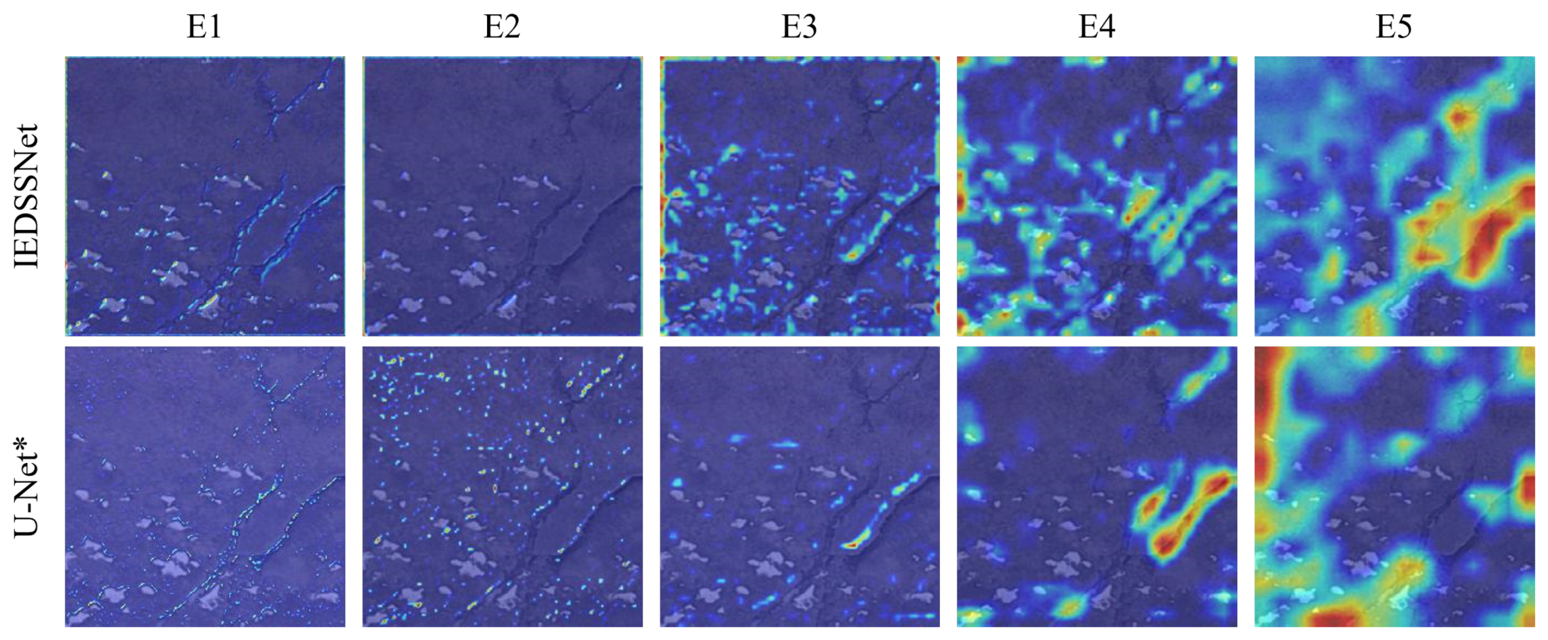
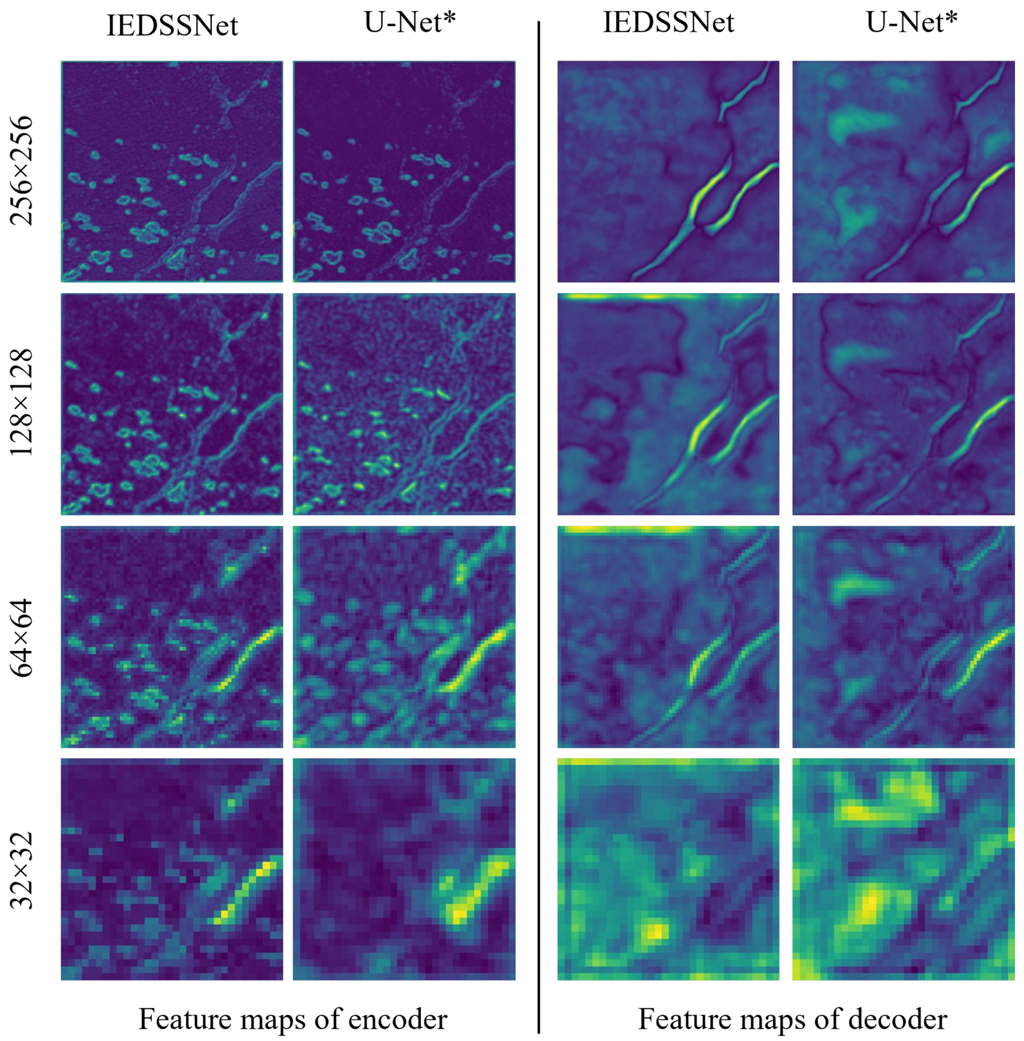
3.3.2. Improvement Analysis of IEDSSNet

To validate the effectiveness of improvements in IEDSSNet, we conducted ablation experiments on the primary test set by incorporating different combinations of blocks into the U-Net model, as shown in

Table 4. Ablation results for different blocks on the primary test set. RSE: residual SE block; MSC: multi-scale skip connection; CCA: channel-wise cross attention.

Network	IOU (%)	Recall (%)	Precision (%)	F1 Score (%)
U-Net*	64.54 (+0.00)	76.13 (+0.00)	80.92 (+0.00)	78.45 (+0.00)
RSE	68.63 (+4.09)	80.60 (+4.47)	82.22 (+1.30)	81.40 (+2.95)
CBAM	67.14 (+2.60)	78.68 (+2.55)	82.07 (+1.15)	80.34 (+1.89)
MSC	67.18 (+2.64)	81.52 (+5.39)	79.25 (−1.67)	80.37 (+1.92)
CCA	67.46 (+2.92)	78.98 (+2.85)	82.22 (+1.30)	80.57 (+2.12)
RSE+MSC	67.26 (+2.72)	79.36 (+3.23)	81.52 (+0.60)	80.42 (+1.97)
RSE+CCA	66.96 (+2.42)	82.78 (+6.65)	77.80 (−3.12)	80.21 (+1.76)
RSE+CBAM	67.00 (+2.46)	78.34 (+2.21)	82.23 (+1.31)	80.24 (+1.79)
CBAM+MSC	67.45 (+2.91)	79.49 (+3.36)	81.66 (+0.74)	80.56 (+2.11)
CBAM+CCA	68.63 (+4.09)	80.78 (+4.65)	82.02 (+1.10)	81.39 (+2.94)
MSC+CCA	67.52 (+2.98)	81.63 (+5.50)	79.62 (−1.30)	80.61 (+2.16)
RSE+CBAM+MSC	68.53 (+3.99)	84.59 (+8.46)	78.30 (-2.62)	81.32 (+2.87)
RSE+CBAM+CCA	67.40 (+2.86)	78.38 (+2.25)	82.79 (+1.87)	80.52 (+2.07)
CBAM+MSC+CCA	67.20 (+2.66)	78.00 (+1.87)	82.90 (+1.98)	80.38 (+1.93)
RSE+MSC+CCA	66.50 (+1.96)	79.72 (+3.59)	80.04 (−0.88)	79.88 (+1.43)
IEDSSNet	69.65 (+5.11)	80.77 (+4.64)	83.49 (+2.57)	82.11 (+3.66)

. The baseline U-Net model used here features a feature map depth of 512 in the fifth stage encoder, matching IEDSSNet’s configuration. To distinguish it from the U-Net model used by Ronneberger et al. [23], which employs a feature map depth of 1024 in the fifth stage encoder, we denote our baseline U-Net model as U-Net* (where * denotes the 512-channel encoder variant).

Integrating different combinations of modules into the baseline U-Net* model enhances overall performance, demonstrating the effectiveness of each improvement block. When individual blocks were added separately, the residual SE block contributed the most to overall performance enhancement, increasing the F1 score and IOU by 2.95% and 4.09%, respectively. The multi-scale skip connection block notably improved recall by 5.39%, albeit with a 1.67% decrease in precision. With the addition of two blocks, the combination of CBAM and channel-wise cross attention contributed the most to performance improvement, resulting in increases of 4.09% and 2.94% in F1 score and IOU, respectively. When three blocks were added, the combination of residual SE block, CBAM, and multi-scale skip connection provided the greatest overall performance improvement, boosting the F1 score and IOU by 3.99% and 2.87%, respectively. This improvement was primarily driven by a significant increase in recall by 8.46% compared to the baseline model. In summary, different block combinations led to varying degrees of improvement in recall, occasionally at the expense of precision. IEDSSNet achieved a more balanced trade-off between recall and precision, demonstrating superior overall performance compared to other incomplete block combinations.

To highlight the advantages brought by the improvement blocks to the proposed IEDSSNet, we performed a visual analysis using attention maps, encoder and decoder feature maps. The encoder was augmented with residual SE blocks and CBAM blocks to aid the model in focusing on crack feature extraction. To illustrate the impact of the improved encoder, attention maps for each stage of both the U-Net* baseline model and the enhanced encoder were visualized, as shown in Figure 10. It is evident that the primary features (E1, E2) of both models focus on more localized and detailed features, such as crack edges and textures. As the network layers deepen, attention gradually shifts towards more global and semantic features, such as crack shape and size. The enhanced encoder primarily focuses on crack edges, whereas U-Net* primarily captures noisy texture features from other complex backgrounds. Moreover, high-level features extracted by the enhanced encoder gradually converge on the crack area, while U-Net* exhibits notably poorer attention towards the overall shape and size of cracks. This implies that our enhancement method is more effective in preserving detailed information, such as crack edges, while also better understanding the overall semantics and structure of cracks.

After averaging feature maps along the channel dimension, we visualize encoder and decoder feature maps of both U-Net* and IEDSSNet, as shown in Figure 11. From the encoder’s feature maps, it is evident that the U-Net*’s feature maps contain more background information, while the crack details are more blurred. In contrast, the enhanced encoder can clearly highlight crack information and reduce unnecessary features during the decoding process. Furthermore, from the feature maps of the decoder, it is evident that the enhanced decoder can more completely and accurately focus on crack targets, while the U-Net* model is relatively weak and incomplete. In comparison, aided by multi-scale skip connections and channel-wise cross attention, the IEDSSNet leverages more semantic information from the encoder and reduces semantic gaps with the decoder features through cross-channel information filtering. This enables the decoder to reconstruct crack features clearly and accurately at the original image resolution.

3.4. Post-Processing and Cataloging Results

The trained IEDSSNet is capable of segmenting landslide surface cracks. Following cropping the DOM, performing model prediction, and stitching the prediction results, we obtained the crack segmentation mask for the entire detection area. However, this mask is inherently coarse and may contain erroneous crack noise. Hence, we refined it using the post-processing methodology detailed in Section 2.3. Morphological closing operations effectively smoothed incomplete holes and boundary artifacts in the crack mask, initially yielding 2879 connected regions. Subsequently, regions containing fewer than 20 pixels were filtered to eliminate isolated noise clusters, reducing the count to 1929 connected regions. Considering potential false positives within these 1929 regions, we refined results using connected-component filtering with an aspect ratio threshold of 2 and area ratio threshold of 0.5, finally retaining 1658 connected regions. Statistical analysis indicated the removal of 1221 connected regions, representing 24.6% of the total crack pixel count. Finally, we quantified the dimensions of each crack at the pixel scale and converted these measurements to real-world distances based on the DOM’s spatial resolution. The vectorized crack inventory for this region is depicted in Figure 12.

In order to evaluate the reliability of the crack inventory results, each crack was meticulously inspected, and vector polygons incorrectly identified as cracks were removed. A total of 1413 correctly detected crack polygons were found, representing the final inventory results, illustrated by the blue mask in Figure 12a. Furthermore, 245 polygons were incorrectly labeled as cracks due to the influence of complex surface backgrounds, such as dark vegetation and snow, as indicated by the green mask in Figure 12a. It is evident that longer cracks in this area are primarily distributed along the rear edge of the landslide, primarily due to the continuous deformation of the landslide. Conversely, a significant number of short cracks exist on both sides of the landslide area edges, likely due to the combined effects of weathering and shear deformation.

Additionally, we demonstrate the effectiveness of the post-processing method using two representative subregions near the rear edge of the landslide, as shown in Figure 12b,c. Following the closing operation, it can be observed that the small cavities within the original predicted crack mask (light sky blue) have been filled, and the edges have become smoother (red). Furthermore, false positive crack masks that do not conform to the shape characteristics of the cracks are filtered out through connected-component analysis, as indicated by the white dashed boxes. The remaining crack masks are then used for subsequent vectorization and attribute measurement. Post-processing significantly refined surface crack masks, yet remained challenged by false positives geometrically resembling true cracks. Overall, our integrated approach achieved automated landslide surface crack detection at 85.22% accuracy.

The relationship between the lengths and widths of the 1413 correctly detected cracks was visualized, as depicted in Figure 13. The cracks range in width from 0.04 m to 0.69 m and in length from 0.06 m to 37.86 m, with most cracks (94.98%) measuring less than 0.2 m wide and most (97.38%) shorter than 5 m. It is noteworthy that in this study, crack length refers to the length of the skeleton within a connected region, while width is defined as the average width of the connected region. This quantification method may differ from reality, as distinguishing multiple cracks in cases of intersecting crack distributions can be challenging. Moreover, small surface crack features, combined with the obscuring effects of complex surface backgrounds, may lead to the detection of cracks as multiple sub-cracks. Additionally, crack geometric measurements are pixel-based, and processes such as skeleton extraction and pixel distance calculation may introduce certain measurement errors. Nonetheless, our proposed crack detection and inventory methods are deemed acceptable, as they can effectively reflect the overall development of cracks within the area.

4. Discussion

4.1. Efficiency of Crack Detection

The efficiency of detecting surface cracks on landslides using a combination of UAVs and deep learning far surpasses that of manual surveys. The crack detection pipeline proposed in this study can automatically and accurately generate a crack inventory. This not only enhances our intuitive understanding of crack distribution but also facilitates the updating and subsequent management of fundamental data for landslide disaster mitigation. Following events such as earthquakes or heavy rainfall, the likelihood of significant deformation leading to landslide instability notably increases. In such emergency scenarios, the efficiency of crack detection pipelines becomes particularly crucial. Timely acquisition of information regarding the distribution of cracks at landslide disaster sites can aid emergency responders in formulating more comprehensive prevention and mitigation strategies.

In practice, obtaining the DOM of the Heifangtai experimental area (as shown in Figure 8) took approximately 83 min. Among this duration, UAV flight data collection consumed around 27 min, while generating the DOM took approximately 56 min. The DOM covered an area of approximately 806,049.8 m², with the crack detection area constituting about ${\displaystyle \frac{1}{8}}$ of the entire DOM. The process of inputting the DOM of the crack detection area into the network to obtain the crack mask took a total of about 14 min. Post-processing and crack cataloging took approximately 10 min. Overall, ignoring some preparatory drone operation time, it was feasible to compile an inventory of surface cracks within a region corresponding to the crack detection area in about 35 min, which is quite promising.

4.2. Impact of Post-Processing Thresholds

Employing filtering thresholds based on geometric properties of connected regions can effectively enhance crack detection accuracy. To assess the specific impact of the aspect ratio and area ratio thresholds on detection performance, we conducted sensitivity analyses on these two key parameters using a set of 1929 connected regions (with 1413 true cracks) obtained after morphological operations and removal of small connected domains (less than 20 pixels), with the results presented in Figure 14. For this evaluation, accuracy is defined as the proportion of correctly detected cracks among all connected regions retained after filtering, while completeness represents the proportion of the original true cracks that were successfully retained after filtering.

As shown in Figure 14a, as the aspect ratio threshold increases, accuracy first rises then decreases—reaching over 80% when the threshold exceeds 2. Meanwhile, completeness shows a significant decreasing trend. This is primarily because higher thresholds more accurately detect true cracks but may miss irregularly shaped (e.g., curved) cracks. For the area ratio, as the threshold increases, accuracy gradually decreases and stabilizes at approximately 73%, while completeness shows a clear upward trend. Smaller area ratios effectively preserve irregularly shaped cracks, and the low completeness indicates that such crack types are rare. Larger area ratios retain most true cracks but introduce more false positives.

To balance accuracy and completeness, a larger aspect ratio threshold and a smaller area ratio threshold were favored for crack filtering. Using an aspect ratio threshold of 2 and area ratio threshold of 0.5, our method detected all true cracks. Despite some remaining false positives, its 85.22% accuracy demonstrates the effectiveness of this approach.

4.3. Limitations and Future Work

While IEDSSNet outperforms comparative methods with an F1 score of 82.11% and IOU of 69.65%, its training dataset remains relatively limited, which may degrade performance when detecting cracks in unseen images. Future work will expand data collection to include more diverse sample types, thereby enhancing the model’s generalization capability and stability. Additionally, it should be noted that crack detection based on UAV optical imagery has limitations in densely vegetated areas, where the vegetation layer prevents optical sensors from capturing ground surface features.

Attention mechanisms have proven effective for crack detection in complex backgrounds. This study incorporates two classic attention mechanisms to improve feature extraction. Future work could benefit from integrating advanced versions of these mechanisms or exploring more sophisticated attention strategies to further enhance network performance [45,46]. Moreover, precise crack annotation remains a labor-intensive task, employing weakly supervised learning methods may alleviate this burden [47].

Although connected-component filtering improves crack detection accuracy, it still yields approximately 15% false positives. Future efforts could implement learning-based strategies or utilize high-resolution digital surface models to mitigate false positives. Overall, this study demonstrates significant engineering potential by integrating UAV and deep learning for automated crack detection in landslide areas, offering a reference framework for analogous scenarios (e.g., detecting permafrost cracks [48] or soil cracks [49]).

5. Conclusions

This study proposes an automated pipeline for detecting surface cracks in landslide areas based on UAV imagery. Its core lies in the development of the IEDSSNet, aimed at segmenting landslide surface cracks from complex surface backgrounds. Introducing CBAM attention and residual SE blocks in the encoder enhances the model’s focus on crack features, while integrating channel-wise cross attention and multi-scale skip connections in the decoder helps fuse features from different stages and reduces the semantic gap in the encoder–decoder architecture. Furthermore, a post-processing procedure for crack segmentation masks and geometric measurements is provided to facilitate instance-level crack cataloging. Based on the results obtained, the conclusions of this study can be summarized as follows:

(1)

The proposed IEDSSNet outperforms other mainstream semantic segmentation networks on the Heifangtai landslide surface crack dataset, with IoU, recall, precision, and F1 scores reaching 69.65%, 80.77%, 83.49%, and 82.11%, respectively. Despite performance degradation under significant illumination variations, it maintains optimal performance with demonstrated generalization capability.

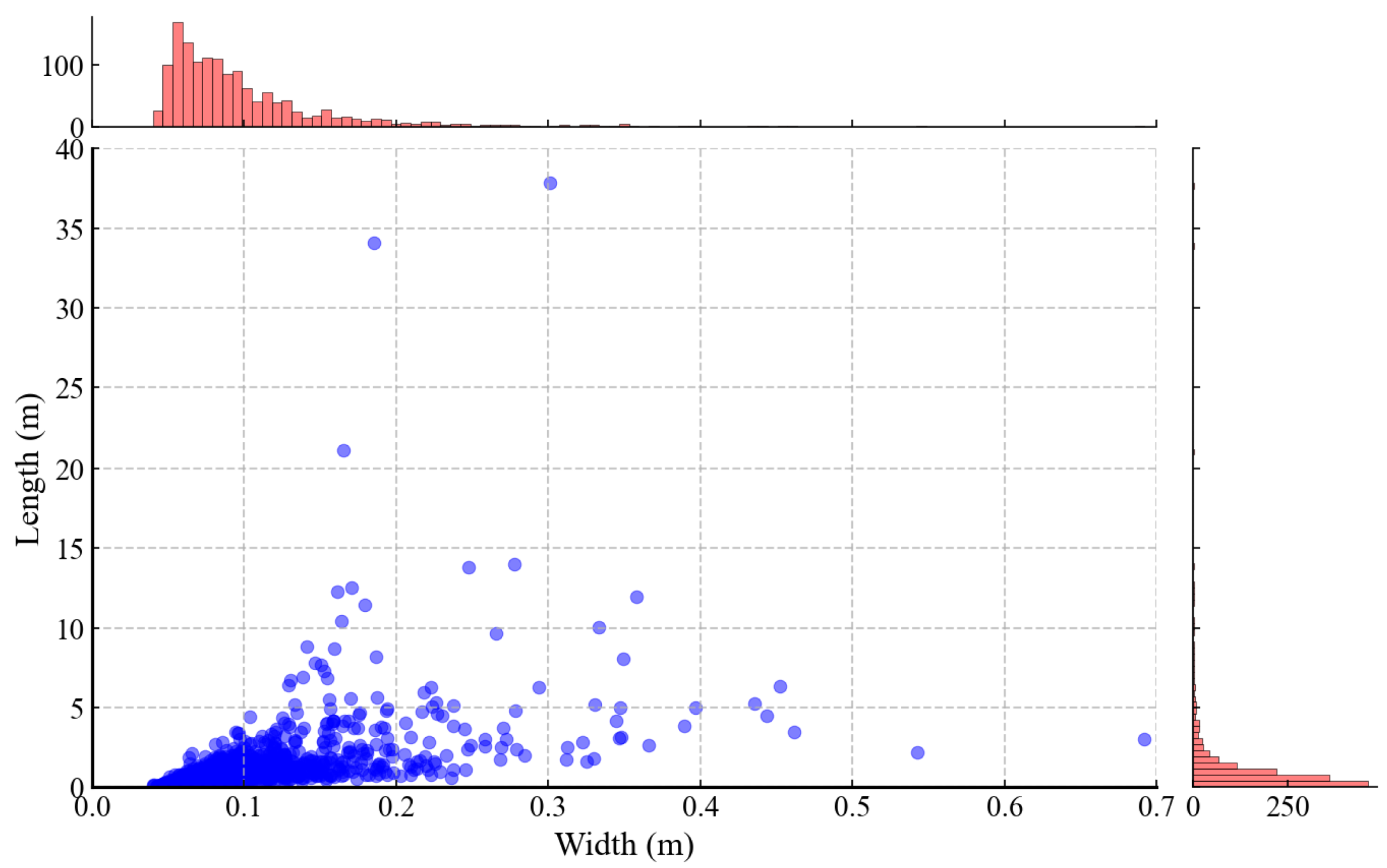
(2)

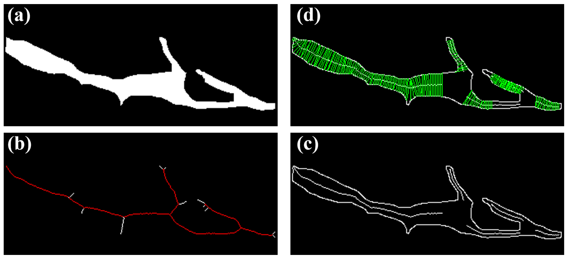
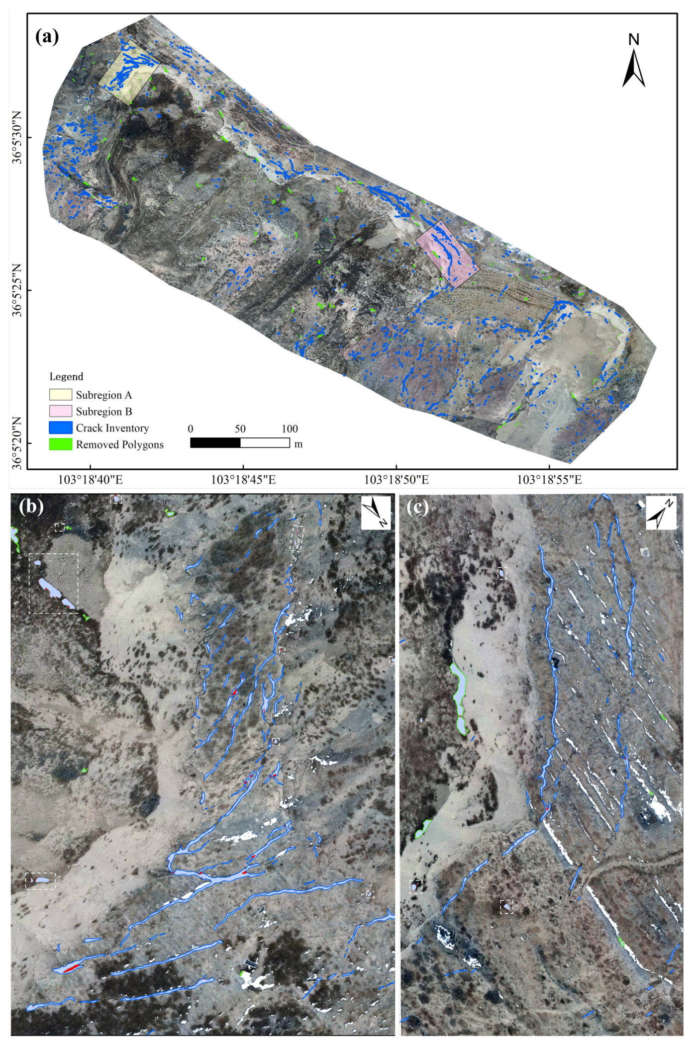
Closing operation and connected-component analysis can effectively suppress false positives. A total of 1658 cracks were automatically cataloged, with a cataloging accuracy of 85.22% following manual inspection. These cracks are predominantly distributed along rear and lateral edges of landslides, with crack widths generally below 0.2 m and lengths concentrated within 5 m.

This proposed method achieves efficient and accurate detection of cracks in complex landslide terrains, providing fundamental data for understanding landslide development processes and demonstrating significant engineering applicability.

References

1. Gariano, S.L.; Guzzetti, F. Landslides in a changing climate. Earth-Sci. Rev. 2016, 162, 227–252. [Google Scholar] [CrossRef]
2. Xu, H.; Shu, B.; Zhang, Q.; Du, Y.; Zhang, J.; We, T.; Xiong, G.; Dai, X.; Wang, L. Site selection for landslide GNSS monitoring stations using InSAR and UAV photogrammetry with analytical hierarchy process. Landslides 2024, 21, 791–805. [Google Scholar] [CrossRef]
3. Xu, H.; Zhang, Q.; Wang, L.; Shu, B.; Du, Y.; Huang, G. Intelligent site selection method for UAV-dropped GNSS landslide monitoring equipment. Acta Geod. Cartogr. Sin. 2024, 53, 1140. [Google Scholar]
4. Wang, H.; Nie, D.; Tuo, X.; Zhong, Y. Research on crack monitoring at the trailing edge of landslides based on image processing. Landslides 2020, 17, 985–1007. [Google Scholar] [CrossRef]
5. Al-Rawabdeh, A.; He, F.; Moussa, A.; El-Sheimy, N.; Habib, A. Using an unmanned aerial vehicle-based digital imaging system to derive a 3D point cloud for landslide scarp recognition. Remote Sens. 2016, 8, 95. [Google Scholar] [CrossRef]
6. Deng, B.; Xu, Q.; Dong, X.; Ju, Y.; Hu, W. Automatic Detection of Deformation Cracks in Slopes Fused with Point Cloud and Digital Image. Geomat. Inf. Sci. Wuhan Univ. 2023, 48, 1296–1311. [Google Scholar]
7. Deng, B.; Xu, Q.; Dong, X.; Li, W.; Wu, M.; Ju, Y.; He, Q. Automatic Method for Detecting Deformation Cracks in Landslides Based on Multidimensional Information Fusion. Remote Sens. 2024, 16, 4075. [Google Scholar] [CrossRef]
8. Fu, H.; Meng, D.; Li, W.; Wang, Y. Bridge crack semantic segmentation based on improved Deeplabv3+. J. Mar. Sci. Eng. 2021, 9, 671. [Google Scholar] [CrossRef]
9. Zheng, X.; Zhang, S.; Li, X.; Li, G.; Li, X. Lightweight bridge crack detection method based on segnet and bottleneck depth-separable convolution with residuals. IEEE Access 2021, 9, 161649–161668. [Google Scholar] [CrossRef]
10. Zou, Q.; Zhang, Z.; Li, Q.; Qi, X.; Wang, Q.; Wang, S. Deepcrack: Learning hierarchical convolutional features for crack detection. IEEE Trans. Image Process. 2018, 28, 1498–1512. [Google Scholar] [CrossRef]
11. Han, C.; Ma, T.; Huyan, J.; Huang, X.; Zhang, Y. CrackW-Net: A novel pavement crack image segmentation convolutional neural network. IEEE Trans. Intell. Transp. Syst. 2021, 23, 22135–22144. [Google Scholar] [CrossRef]
12. Lau, S.L.; Chong, E.K.; Yang, X.; Wang, X. Automated pavement crack segmentation using u-net-based convolutional neural network. IEEE Access 2020, 8, 114892–114899. [Google Scholar] [CrossRef]
13. Loverdos, D.; Sarhosis, V. Automatic image-based brick segmentation and crack detection of masonry walls using machine learning. Autom. Constr. 2022, 140, 104389. [Google Scholar] [CrossRef]
14. Chen, K.; Reichard, G.; Xu, X.; Akanmu, A. Automated crack segmentation in close-range building façade inspection images using deep learning techniques. J. Build. Eng. 2021, 43, 102913. [Google Scholar] [CrossRef]
15. Zhou, S.; Canchila, C.; Song, W. Deep learning-based crack segmentation for civil infrastructure: Data types, architectures, and benchmarked performance. Autom. Constr. 2023, 146, 104678. [Google Scholar] [CrossRef]
16. Yuan, Y.; Ge, Z.; Su, X.; Guo, X.; Suo, T.; Liu, Y.; Yu, Q. Crack length measurement using convolutional neural networks and image processing. Sensors 2021, 21, 5894. [Google Scholar] [CrossRef]
17. Xu, J.J.; Zhang, H.; Tang, C.S.; Cheng, Q.; Liu, B.; Shi, B. Automatic soil desiccation crack recognition using deep learning. Geotechnique 2022, 72, 337–349. [Google Scholar] [CrossRef]
18. Pham, M.V.; Ha, Y.S.; Kim, Y.T. Automatic detection and measurement of ground crack propagation using deep learning networks and an image processing technique. Measurement 2023, 215, 112832. [Google Scholar] [CrossRef]
19. Yu, D.; Ji, S.; Li, X.; Yuan, Z.; Shen, C. Earthquake crack detection from aerial images using a deformable convolutional neural network. IEEE Trans. Geosci. Remote Sens. 2022, 60, 4412012. [Google Scholar] [CrossRef]
20. Tao, T.; Han, K.; Yao, X.; Chen, X.; Wu, Z.; Yao, C.; Tian, X.; Zhou, Z.; Ren, K. Identification of ground fissure development in a semi-desert aeolian sand area induced from coal mining: Utilizing UAV images and deep learning techniques. Remote Sens. 2024, 16, 1046. [Google Scholar] [CrossRef]
21. Sandric, I.; Chitu, Z.; Ilinca, V.; Irimia, R. Using high-resolution UAV imagery and artificial intelligence to detect and map landslide cracks automatically. Landslides 2024, 21, 2535–2543. [Google Scholar] [CrossRef]
22. Cheng, Z.; Gong, W.; Jaboyedoff, M.; Chen, J.; Derron, M.H.; Zhao, F. Landslide Identification in UAV Images Through Recognition of Landslide Boundaries and Ground Surface Cracks. Remote Sens. 2025, 17, 1900. [Google Scholar] [CrossRef]
23. Ronneberger, O.; Fischer, P.; Brox, T. U-net: Convolutional networks for biomedical image segmentation. In Proceedings of the Medical Image Computing and Computer-Assisted Intervention—MICCAI 2015: 18th International Conference, Munich, Germany, 5–9 October 2015; Proceedings, Part III 18. Springer: Berlin/Heidelberg, Germany, 2015; pp. 234–241. [Google Scholar]
24. Zhao, H.; Shi, J.; Qi, X.; Wang, X.; Jia, J. Pyramid scene parsing network. In Proceedings of the IEEE Conference on Computer Vision and Pattern Recognition, Honolulu, HI, USA, 21–26 July 2017; pp. 2881–2890. [Google Scholar]
25. Chen, L.C.; Zhu, Y.; Papandreou, G.; Schroff, F.; Adam, H. Encoder-decoder with atrous separable convolution for semantic image segmentation. In Proceedings of the European Conference on Computer Vision (ECCV), Munich, Germany, 8–14 September 2018; pp. 801–818. [Google Scholar]
26. Wang, H.; Cao, P.; Wang, J.; Zaiane, O.R. Uctransnet: Rethinking the skip connections in u-net from a channel-wise perspective with transformer. In Proceedings of the AAAI Conference on Artificial Intelligence, Virtual, 22 February–1 March 2022; Volume 36, pp. 2441–2449. [Google Scholar]
27. Liu, Z.; Cao, Y.; Wang, Y.; Wang, W. Computer vision-based concrete crack detection using U-net fully convolutional networks. Autom. Constr. 2019, 104, 129–139. [Google Scholar] [CrossRef]
28. Woo, S.; Park, J.; Lee, J.Y.; Kweon, I.S. Cbam: Convolutional block attention module. In Proceedings of the European Conference on Computer Vision (ECCV), Munich, Germany, 8–14 September 2018; pp. 3–19. [Google Scholar]
29. Zhang, K.; Sun, M.; Han, T.X.; Yuan, X.; Guo, L.; Liu, T. Residual networks of residual networks: Multilevel residual networks. IEEE Trans. Circuits Syst. Video Technol. 2017, 28, 1303–1314. [Google Scholar] [CrossRef]
30. Ates, G.C.; Mohan, P.; Celik, E. Dual cross-attention for medical image segmentation. Eng. Appl. Artif. Intell. 2023, 126, 107139. [Google Scholar] [CrossRef]
31. Wazir, S.; Fraz, M.M. HistoSeg: Quick attention with multi-loss function for multi-structure segmentation in digital histology images. In Proceedings of the 2022 12th International Conference on Pattern Recognition Systems (ICPRS), Saint-Etienne, France, 7–10 June 2022; pp. 1–7. [Google Scholar]
32. Blum, H. Biological shape and visual science (Part I). J. Theor. Biol. 1973, 38, 205–287. [Google Scholar] [CrossRef]
33. Bai, X.; Latecki, L.J. Discrete skeleton evolution. In Proceedings of the Energy Minimization Methods in Computer Vision and Pattern Recognition: 6th International Conference, EMMCVPR 2007, Ezhou, China, 27–29 August 2007; Proceedings 6. Springer: Berlin/Heidelberg, Germany, 2007; pp. 362–374. [Google Scholar]
34. Ong, J.C.; Ismadi, M.Z.P.; Wang, X. A hybrid method for pavement crack width measurement. Measurement 2022, 197, 111260. [Google Scholar] [CrossRef]
35. Zhang, Q.; Bai, Z.; Huang, G.; Kong, J.; Du, Y.; Wang, D.; Jing, C.; Xie, W. Innovative landslide disaster monitoring: Unmanned aerial vehicle-deployed GNSS technology. Geomat. Nat. Hazards Risk 2024, 15, 2366374. [Google Scholar] [CrossRef]
36. Huang, G.; Wang, D.; Du, Y.; Zhang, Q.; Bai, Z.; Wang, C. Deformation feature extraction for GNSS landslide monitoring series based on robust adaptive sliding-window algorithm. Front. Earth Sci. 2022, 10, 884500. [Google Scholar] [CrossRef]
37. Loshchilov, I.; Hutter, F. Sgdr: Stochastic gradient descent with warm restarts. arXiv 2016, arXiv:1608.03983. [Google Scholar]
38. Goyal, P.; Dollár, P.; Girshick, R.; Noordhuis, P.; Wesolowski, L.; Kyrola, A.; Tulloch, A.; Jia, Y.; He, K. Accurate, large minibatch sgd: Training imagenet in 1 hour. arXiv 2017, arXiv:1706.02677. [Google Scholar]
39. Kingma, D.P.; Ba, J. Adam: A method for stochastic optimization. arXiv 2014, arXiv:1412.6980. [Google Scholar]
40. Everingham, M.; Van Gool, L.; Williams, C.K.; Winn, J.; Zisserman, A. The pascal visual object classes (voc) challenge. Int. J. Comput. Vis. 2010, 88, 303–338. [Google Scholar] [CrossRef]
41. Lin, T.Y.; Maire, M.; Belongie, S.; Hays, J.; Perona, P.; Ramanan, D.; Dollár, P.; Zitnick, C.L. Microsoft coco: Common objects in context. In Proceedings of the Computer Vision—ECCV 2014: 13th European Conference, Zurich, Switzerland, 6–12 September 2014; Proceedings, Part V 13. Springer: Berlin/Heidelberg, Germany, 2014; pp. 740–755. [Google Scholar]
42. Oktay, O.; Schlemper, J.; Folgoc, L.L.; Lee, M.; Heinrich, M.; Misawa, K.; Mori, K.; McDonagh, S.; Hammerla, N.Y.; Kainz, B.; et al. Attention u-net: Learning where to look for the pancreas. arXiv 2018, arXiv:1804.03999. [Google Scholar]
43. Zhou, Z.; Rahman Siddiquee, M.M.; Tajbakhsh, N.; Liang, J. Unet++: A nested u-net architecture for medical image segmentation. In Proceedings of the Deep Learning in Medical Image Analysis and Multimodal Learning for Clinical Decision Support: 4th International Workshop, DLMIA 2018, and 8th International Workshop, ML-CDS 2018, Held in Conjunction with MICCAI 2018, Granada, Spain, 20 September 2018; Proceedings 4. Springer: Berlin/Heidelberg, Germany, 2018; pp. 3–11. [Google Scholar]
44. Huang, H.; Lin, L.; Tong, R.; Hu, H.; Zhang, Q.; Iwamoto, Y.; Han, X.; Chen, Y.; Wu, J.U. 3+: A full-scale connected UNet for medical image segmentation. arXiv 2020, arXiv:2004.08790. [Google Scholar]
45. Park, J.; Woo, S.; Lee, J.Y.; Kweon, I.S. Bam: Bottleneck attention module. arXiv 2018, arXiv:1807.06514. [Google Scholar]
46. Wang, G.; Cheng, G.; Zhou, P.; Han, J. Cross-level attentive feature aggregation for change detection. IEEE Trans. Circuits Syst. Video Technol. 2023, 34, 6051–6062. [Google Scholar] [CrossRef]
47. Inoue, Y.; Nagayoshi, H. Weakly-supervised crack detection. IEEE Trans. Intell. Transp. Syst. 2023, 24, 12050–12061. [Google Scholar] [CrossRef]
48. Kaiser, S.; Boike, J.; Grosse, G.; Langer, M. The Potential of UAV Imagery for the Detection of Rapid Permafrost Degradation: Assessing the Impacts on Critical Arctic Infrastructure. Remote Sens. 2022, 14, 6107. [Google Scholar] [CrossRef]
49. Xu, J.J.; Zhang, H.; Tang, C.S.; Cheng, Q.; Tian, B.-G.; Liu, B.; Shi, B. Automatic soil crack recognition under uneven illumination condition with the application of artificial intelligence. Eng. Geol. 2022, 296, 106495. [Google Scholar] [CrossRef]
Figure 1. Workflow for detecting surface cracks in landslides from UAV images.
Remotesensing 17 02150 g001
Figure 2. Overall architecture of IEDSSNet for landslide surface crack semantic segmentation.
Remotesensing 17 02150 g002
Figure 3. Architecture of CBAM block. (a) CBAM block; (b) channel attention module; (c) spatial attention module.
Remotesensing 17 02150 g003
Figure 4. Architecture of residual SE block. (a) Residual SE block; (b) SE block.
Remotesensing 17 02150 g004
Figure 5. Illustration of the multi-scale skip connection block.
Remotesensing 17 02150 g005
Figure 6. Diagram of the channel-wise cross attention block.
Remotesensing 17 02150 g006
Figure 7. Schematic diagram of crack length and width measurement. (a) Crack mask; (b) crack skeletonization and length measurement; (c) removal of intersecting regions; (d) measurement of crack width.
Remotesensing 17 02150 g007
Figure 8. General information of the study area: (a) location of the study area; (b) DOM of auxiliary test area (1.5 cm/pixel, 31 December 2023); (c) DOM covering training and crack detection areas (2 cm/pixel, 15 February 2023). The base maps are sourced from Google imagery.
Remotesensing 17 02150 g008
Figure 9. Results of different models. From left to right: original image; ground truth; U-Net; Attention U-Net; U-Net++; U-Net3+; PSPNet; UCTransNet; Deeplabv3+; DeepCrack; Crack-CADNet; IEDSSNet. Numbers 1–6 denote crack sample identifiers.
Remotesensing 17 02150 g009
Figure 10. Visualization and comparison of attention maps corresponding to different stages in the encoder.
Remotesensing 17 02150 g010
Figure 11. Visualization and comparison of feature maps between U-Net* and IEDSSNet.
Remotesensing 17 02150 g011
Figure 12. Crack inventory results and visualization of the post-processing process. (a) Entire crack detection area; (b) subregion A; (c) subregion B.
Remotesensing 17 02150 g012
Figure 13. Relationship diagram of crack length and width within the experimental area. Blue circles represent individual crack measurements; Red bars on top and right axes indicate frequency distributions of crack width and length, respectively.
Remotesensing 17 02150 g013
Figure 14. Accuracy and completeness under different filtering thresholds. (a) Aspect ratio; (b) area ratio.
Remotesensing 17 02150 g014