Retrieval of Ocean Surface Currents by Synergistic Sentinel-1 and SWOT Data Using Deep Learning

Abstract

A reliable ocean surface current (OSC) estimate is difficult to retrieve from synthetic aperture radar (SAR) data due to the challenge of accurately partitioning the Doppler shifts induced by wind waves and OSC. Recent research on SAR-based OSC retrieval is typically based on the assumption that the SAR Doppler shifts caused by wind waves and OSC are linearly superimposed. However, this assumption may lead to large errors in regions where nonlinear wave–current interactions are significant. To address this issue, we developed a novel deep learning model, OSCNet, for OSC retrieval. The model leverages Sentinel-1 Interferometric Wide (IW) Level 2 Ocean products collected from July 2023 to September 2024, combined with wave data from the European Centre for Medium-Range Weather Forecasts (ECMWF) and geostrophic currents from newly available SWOT Level 3 products. The OSCNet model is optimized by refining input ocean surface physical parameters and introducing a ResNet structure. Moreover, the Normalized Radar Cross-Section (NRCS) is incorporated to account for wave breaking and backscatter effects on Doppler shift estimates. The retrieval performance of the OSCNet model is evaluated using SWOT data. The mean absolute error (MAE) and root mean square error (RMSE) are found to be 0.15 m/s and 0.19 m/s, respectively. This result demonstrates that the OSCNet model enhances the retrieval of OSC from SAR data. Furthermore, a mesoscale eddy detected in the OSC map retrieved by OSCNet is consistent with the collocated sea surface chlorophyll-a observation, demonstrating the capability of the proposed method in capturing the variability of mesoscale eddies.

1. Introduction

Ocean surface currents (OSCs) play a pivotal role in physical oceanography, marine ecosystems, and climate studies [1,2]. The monitoring of OSC is critical for multiple marine activities, particularly in vessel trajectory planning, contaminant transport prediction, life-saving emergency deployments, and offshore engineering [3,4,5]. Several remote sensing techniques have been advanced to estimate OSC, with Synthetic Aperture Radar (SAR) being a prominent technique due to its ability to provide high-resolution images in all weather conditions and at any time of day or night.

There are two methods for SAR OSC retrieval: along-track interferometry (ATI), first introduced in 1987 [6], and Doppler centroid anomaly (DCA), originally formulated in 1979 [7]. ATI-derived currents have been shown to be more accurate than DCA-based estimates in long baseline configurations [8]. However, the ATI technique requires two complex SAR images from two separate antennas aligned in the flight direction to retrieve ocean surface velocity. The operational unavailability of this configuration in most of the SAR satellites hampers its application. In contrast, the Doppler centroid can be directly estimated from any single-channel data, enabling numerous satellites capable of retrieving OSC velocities using the DCA method. Consequently, the potential for measuring OSC using the DCA technique has been validated through various experiments using Envisat/ASAR [9,10,11,12], Sentinel-1 (S1) [13,14,15,16], and GF-3 SAR data [17,18,19] since the method was systematically introduced in 2005 [20].

The Doppler centroid recorded by SAR includes the sea surface motion caused by waves and OSC in the radial direction of the radar [21]. Research on the accurate estimation of OSC has made some progress over the past decade, with the assumption that wind-wave-induced motion and currents are linearly separable. Specifically, the wind-induced component is first estimated using empirical geophysical model functions (GMFs) such as CDOP [22] and its advanced versions, CDOP-S [21], CDOP-3S [21], and CDOP3SiX [23]. This component is then subtracted from the total velocity to obtain the OSC estimates. All of these GMFs are developed in regions where OSCs are weak or absent, and the wave–current interactions are neglected. However, wave–current interactions have a significant impact on the sea state [24,25], and the retrieval of OSCs using these GMFs may lead to large errors in regions where nonlinearity and coupling between wind, waves, and currents are pronounced. As a result, the partitioning of the Doppler frequency shift to the different contributions and obtaining a reliable estimate of the OSC remain challenging problems.

Recent advances in artificial intelligence (AI) have introduced novel methodologies for oceanographic applications [26,27]. These include the detection of ocean phenomena, such as eddies [28] and internal waves [29], and the inversion of ocean parameters [30,31] from remote sensing data. Several studies have investigated AI techniques to estimate OSCs directly from SAR observations by modeling the complex relationships between Doppler signatures and environmental conditions. Zhou et al. [32] developed an XGBoost-based algorithm to retrieve OSC radial velocity from S1 SAR data under tropical cyclone conditions, demonstrating its robustness in extreme sea states. Yang et al. [33] systematically quantified the effects of wind and waves on Doppler frequency shifts, enabling more accurate environmental corrections for SAR-based OSC retrieval. Shao et al. [34] introduced a deep learning framework for retrieving range currents from Sentinel-1 SAR ocean products, achieving enhanced precision in low-to-moderate sea states. Bai et al. [35] proposed a machine learning model utilizing Sentinel-1 products, incorporating matched reference data to achieve higher accuracy and robustness than conventional methods across diverse sea conditions. However, these approaches typically rely on either numerical models or high-frequency (HF) radar data, such as ground truth. Numerical models often possess coarser spatial resolutions than required, whereas HF radar data are limited to nearshore regions with sparse and fixed spatial coverage. Fortunately, the launch of the Surface Water and Ocean Topography (SWOT) satellite mission has yielded unprecedented high-resolution measurements of global mesoscale and submesoscale features, providing a valuable opportunity for large-area, high-resolution OSC monitoring [36,37,38].

In this paper, we present a novel method for retrieving OSCs using synergistic S1 and SWOT data via deep learning. Unlike conventional methods that assume a linear separation of wind and currents, our model utilizes a neural network to directly learn the nonlinear relationships among wind, waves, and currents. Specifically, we feed the S1-measured ocean surface radial velocity and wind-wave information into the model, while SWOT-derived currents serve as ground truth. Furthermore, we incorporate the Normalized Radar Cross-Section (NRCS) in the input layer to account for the modulation of the Doppler centroid by wave breaking and backscatter gradients. The synergistic combination of S1 SAR and SWOT data enhances OSC retrieval by expanding the spatial coverage of SWOT observations. Additionally, the complementary temporal characteristics of the two datasets improve time efficiency, allowing for the more frequent and comprehensive monitoring of OSCs.

The remainder of this article is organized as follows. Section 2 introduces the study area and datasets, followed by a presentation of the methodology in Section 3. The experimental results are presented in Section 4. Section 5 provides a detailed discussion, while Section 6 concludes this study.

2. Study Area and Datasets

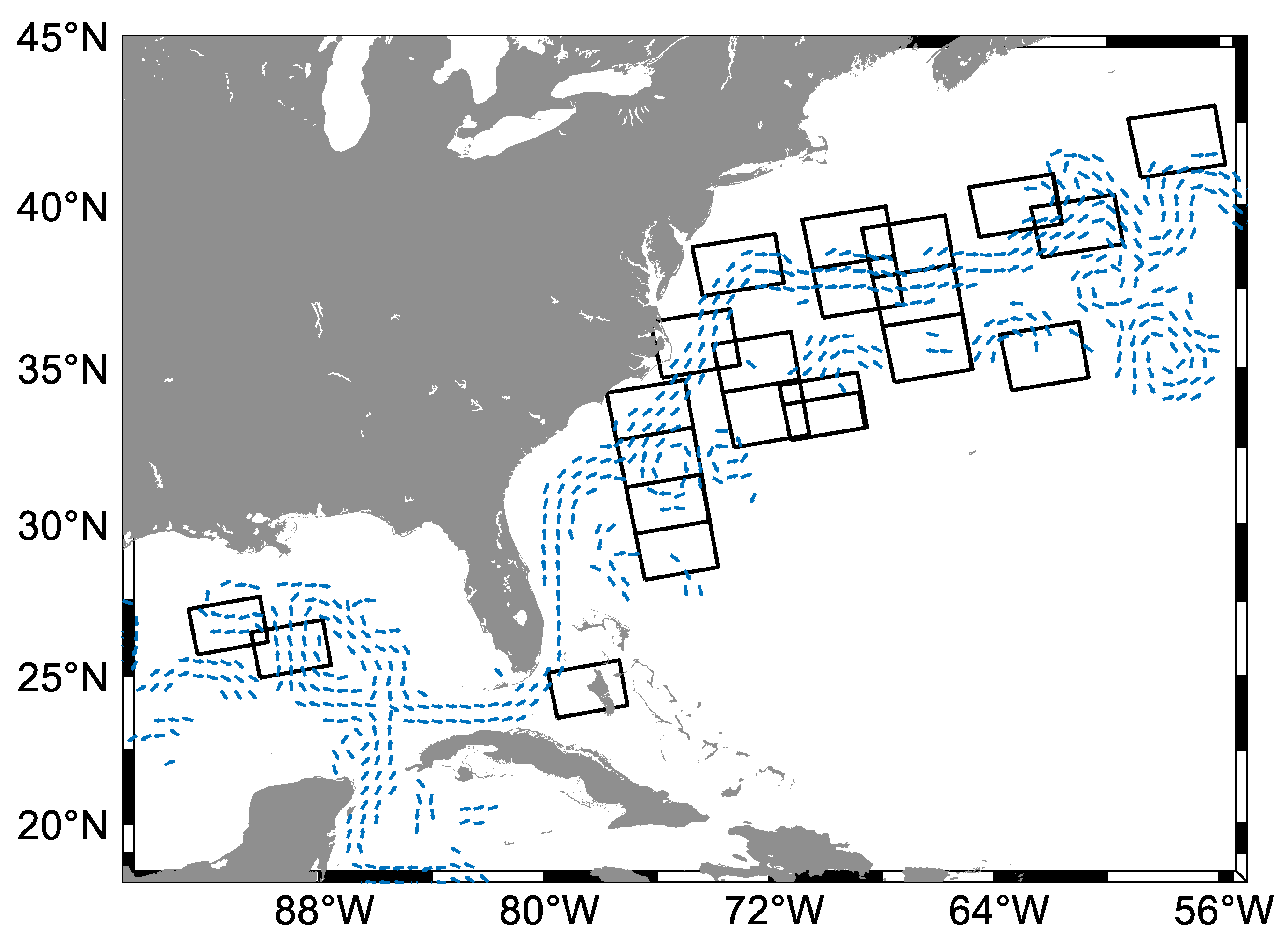
2.1. Study Area

The study area is primarily located in the region of the Gulf Stream, as shown in Figure 1. The Gulf Stream, a strong western boundary current with velocities exceeding 1.5 m/s, plays a critical role in North Atlantic circulation and significantly impacts oceanic heat transport and climate dynamics. In addition to its strength, the wave–current interaction in this region is particularly pronounced due to the high velocities and energetic wave dynamics [39,40]. The wave–current interaction can modify both the characteristics of surface waves and the structure of the underlying currents, making the Gulf Stream an ideal region for OSC retrieval studies [41].

2.2. Datasets

The datasets used in this study include S1 ocean product (referred to as OCN) data, European Centre for Medium-Range Weather Forecasts (ECMWF) ERA5 reanalysis data, and SWOT Level-3 (L3) data. Each dataset is described in detail below, and its main parameters are summarized in

Table 1. Main parameters of the dataset used in this study.

Data Source	Data Set (Unit)	Resolution	Swath	Data Provider
S1 IW OCN	Surface radial velocity (m/s), wind speed (m/s), Stokes drift (m/s), platform heading (deg)	1 km	300 km	ESA/Copernicus
ERA5 Reanalysis	Significant height (m), mean period (s), and mean direction (deg) of wind waves; total swells and mean waves	0.25°	–	ECMWF
SWOT L3	Geostrophic currents (m/s)	2 km	128 km	AVISO/DUACS

.

2.2.1. S1 OCN Data

The European Space Agency (ESA) has, for the first time globally, developed a Level 2 OCN product based on S1 SAR data. The OCN products integrate two or three key geophysical parameters. These include radial velocity measurements (RVL) obtained through the Doppler DCA technique applied to Sentinel-1 Single-Look Complex (SLC) SAR images, along with ocean surface wind field (OWI) and ocean swell wave spectra (OSW). In this study, we utilize the ocean surface radial velocity and surface Stokes drift provided by the RVL data, as well as the wind vector and NRCS supplied by the OWI data.

2.2.2. ECMWF ERA5 Reanalysis Data

The ECMWF ERA5 reanalysis data is the fifth-generation atmospheric reanalysis dataset released in 2019. In this study, the significant height of wind waves $H_{ww}$, significant height of total swell $H_{ts}$, significant height of combined wind waves and swell $H_{wws}$, mean period of wind waves $T_{ww}$, mean period of total swell $T_{ts}$, mean wave period $T_{wws}$, mean direction of wind waves ${\varphi }_{ww}$, mean direction of total swell ${\varphi }_{ts}$, and mean wave direction ${\varphi }_{wws}$ provided by ERA5 are used.

2.2.3. SWOT L3 Data

The SWOT mission is a partnership between the physical oceanography and hydrology communities, providing the first comprehensive mapping of terrestrial surface water bodies while capturing high-resolution measurements of sea surface height variations [37]. The L3 product provides a rigorous geophysical correction of the sea surface height derived from the Ka-band radar interferometer (KaRIn) measurements. In this study, the geostrophic currents derived from the sea surface height anomalies are utilized.

3. Methodology

The framework of the proposed method is illustrated in Figure 2. It primarily consists of a preprocessing module, a dataset construction module, and an OSC retrieval network. Each component is described in detail below.

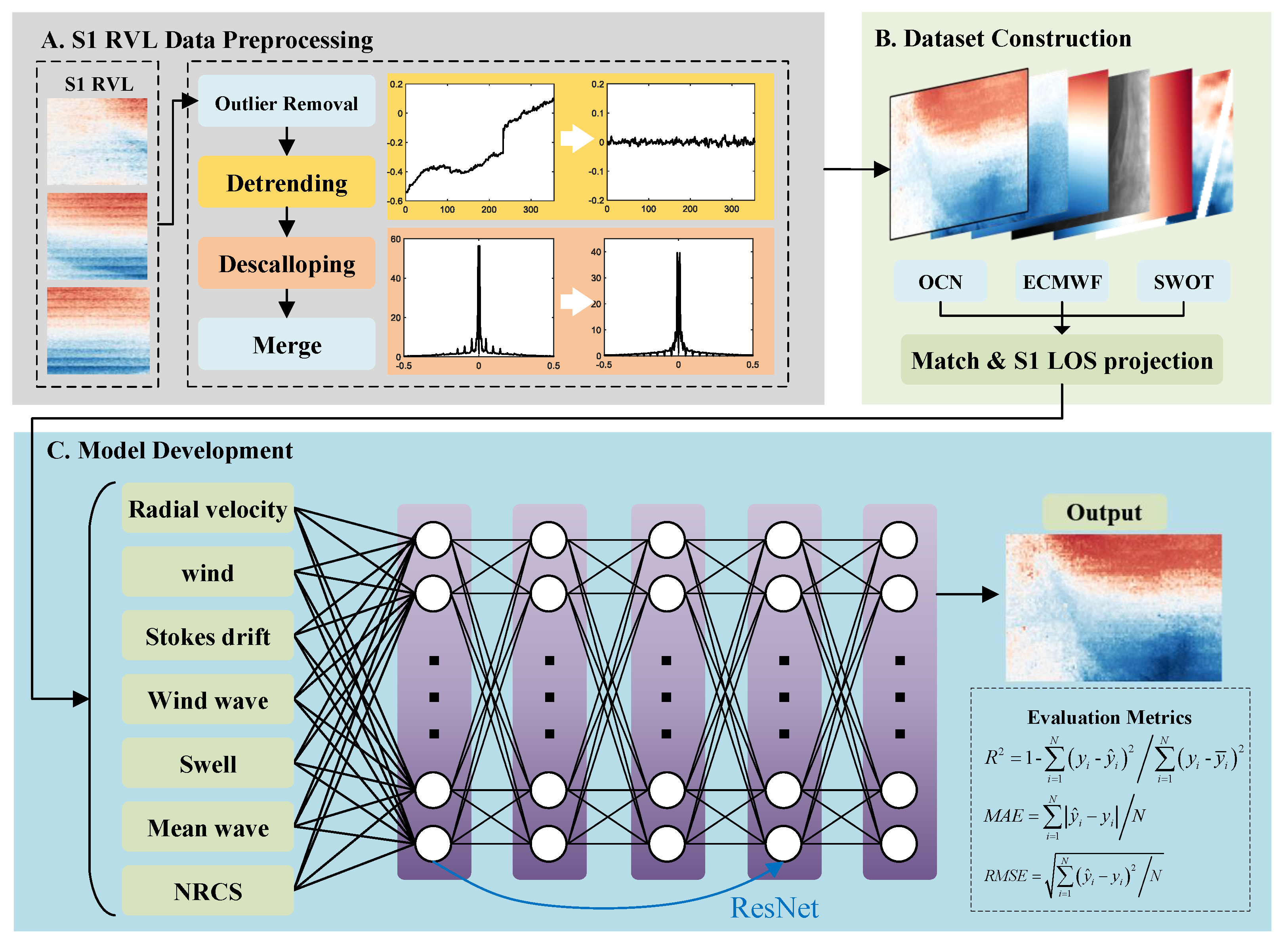
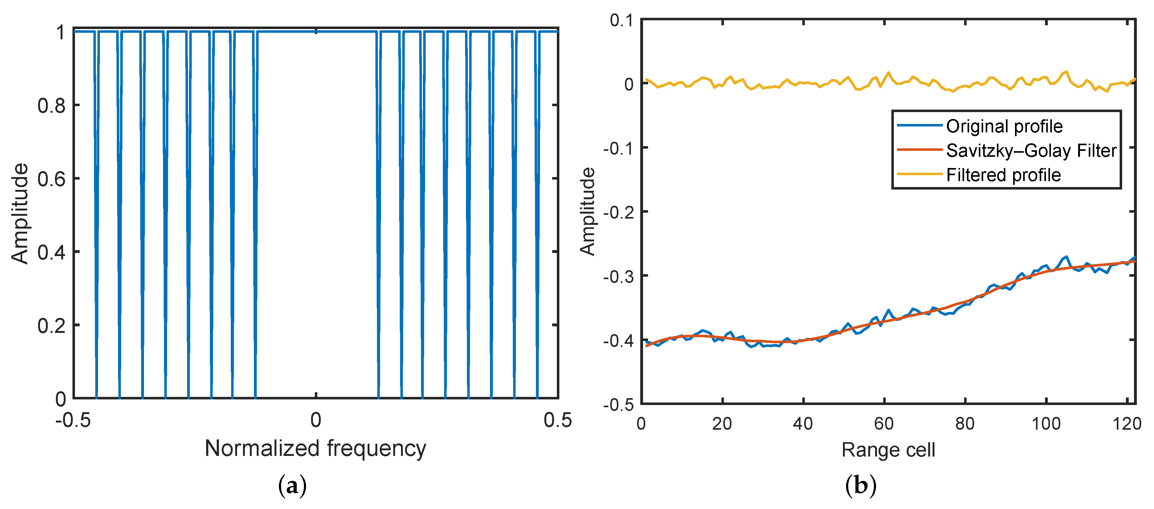
3.1. S1 RVL Data Preprocessing

In the DCA framework, OSC estimation mainly relies on the Doppler centroid of the backscattered radar signal from the moving ocean surface. The Doppler centroid $f_{dc}$ consists of multiple contributing sources, as shown by

$$f_{dc}=f_{geo}+f_{sca}+f_{em}+f_{curr}+f_{ss}+f_{err}$$

(1)

where $f_{geo}$ arises from the relative velocity of the satellite and rotating Earth, $f_{sca}$ denotes the scalloping distortion caused by SAR antenna scanning in the TOPSAR mode, $f_{em}$ stands for the electronic pointing error of the antenna, and $f_{curr}$ corresponds the Doppler frequency shift generated by the OSC. For strong currents, such as the Gulf Stream, the OSC is dominated by geostrophic currents. Additionally, $f_{ss}$ denotes sea-state-induced motions, while $f_{err}$ encompasses all unknown or residual errors. Reliable OSC estimation demands a thorough compensation of all non-current-related Doppler effects. After this, the OSC radial velocity is determined by

$$U_{curr}=-{\displaystyle \frac{\pi f_{curr}}{k_{e}sin{\theta }_i}}$$

(2)

where $k_e$ denotes the radar electromagnetic wave number, and ${\theta }_i$ represents the incidence angle.

The S1 Interferometric Wide (IW) SAR RVL product comprises three swaths. We processed each swath individually and then merged them to produce an ocean surface radial velocity map that aligns with the SAR image’s coverage. For each swath, the standard deviation of the ocean surface radial velocity estimates is first calculated, and pixels with a standard deviation exceeding 0.5 m/s are excluded to eliminate the influence of artificial targets such as ships. Next, a Savitzky–Golay filter was applied to remove trends along the range direction of the RVL data caused by antenna mispointing. Finally, the azimuthal frequency spectra of RVL data were analyzed, and a notch filter was constructed based on the antenna scanning period to mitigate scalloping effects. The constructed azimuthal and range filters are shown in Figure 3. Figure 3a shows a notch filter utilized for azimuthal descalloping, with the horizontal axis representing the azimuthal normalized frequency. Figure 3b illustrates a Savitzky–Golay filter used for range detrending, where the blue solid line and yellow solid line represent the range profiles before and after filtering, respectively, and the red solid line represents the filter.

3.2. Dataset Construction

To construct a comprehensive dataset, we integrated four distinct products: OCN RVL data, OCN OWI data, ECMWF ERA5 data, and SWOT data. Given the heterogeneous spatial resolutions inherent to these datasets, the initial step involved harmonizing their spatial grids to ensure uniformity across all input features and the target variable. Specifically, the OCN RVL and OCN OWI products provide high-resolution measurements of ocean surface radial velocity and wind-related parameters directly related to the resolution of the S1 SLC data and the resolution of S1 Ground-Range-Detected (GRD) data, respectively. The ECMWF ERA5 dataset provides wave parameters with a spatial resolution of 0.5° × 0.5°. We resampled the geophysical parameters from the RVL and OWI components to match the SWOT data, which are provided on a geographically fixed, swath-aligned 2 km × 2 km grid. The S1 RVL and OWI products were bilinearly interpolated to the 2 km SWOT grid, preserving spatial gradients while suppressing high-frequency noise. The ERA5 wave parameters were upsampled to 2 km using bicubic spline interpolation to enhance the representation of submesoscale wave–current interactions.

Once the spatial grids were harmonized, we projected the geostrophic current vector ${\mathbf{u}}_g=\left(u_g,v_g\right)$ onto the S1 SAR radial direction to obtain the geostrophic radial velocity $u_{g,r}$. This projection was achieved by calculating the inner product of the geostrophic velocity vector with the radar’s radial unit vector $\widehat{\mathbf{r}}$, which can be expressed as

$$u_{g,r}={\mathbf{u}}_g·\widehat{\mathbf{r}}=u_{g}sin\left(\varphi -3\pi /\phantom{3\pi 2}2\right)+v_{g}cos\left(\varphi -3\pi /\phantom{3\pi 2}2\right)$$

(3)

where $\varphi$ represents the platform heading from the north. Similarly, we utilized significant wave heights and mean periods for both wind waves and swell from the ECMWF ERA5 data to estimate the orbital velocities of each wave component based on linear wave theory. The resulting orbital velocity vectors were then projected onto the radar radial direction, yielding a radial wave orbital velocity component, as expressed in Equation (4):

$$u_{x,r}={\displaystyle \frac{\pi H_x}{T_x}}cos{\varphi }_r^x$$

(4)

where $H_x$ is the significant of waves ($H_{ww}$, $H_{ts}$, and $H_{wws}$), and $T_x$ is the period of waves ($T_{ww}$, $T_{ts}$, and $T_{wws}$). ${\varphi }_r^x$ is the wave direction with respect to the SAR azimuth direction.

Finally, we performed feature-wise normalization using global statistics across all matchups to standardize the range of input features, ensuring the more efficient training of deep learning models. In addition, we handled any missing values or outliers through interpolation techniques and outlier detection to improve data quality and reliability. The cleaned input features (including resampled OCN RVL, OCN OWI, and ECMWF ERA5 wave parameters) were then paired with the corresponding SWOT measurements, creating a robust dataset suitable for supervised deep learning.

3.3. Model Development

3.3.1. Architecture of the Model

In this article, we develop a model for OSC retrieval based on deep neural networks, which is named OSCNet. The model is architected as a multi-layer perceptron (MLP) comprising five hidden layers, with neuron counts symmetrically ascending and subsequently descending. This layered configuration is strategically designed to facilitate the progressive abstraction and hierarchical extraction of complex features from the integrated datasets. Each hidden layer is succeeded by an activation function, which introduces essential nonlinearity and enhances the network’s capability to learn and model complex nonlinear relationships among ocean surface wind, waves, and currents.

To enhance this deep MLP architecture and overcome common challenges in training deep networks, OSCNet incorporates a key architectural innovation inspired by the residual neural network (ResNet) concept, a deep learning architecture in which the layers learn residual functions with reference to the layer’s inputs [42]. In OSCNet, this is implemented by creating a dedicated pathway that directly propagates the initial input to the fifth hidden layer, where it is added to the output of that layer. This ResNet-style architectural enhancement is particularly advantageous for studying the intricate interactions among ocean surface wind, waves, and currents. By mitigating the vanishing gradient problem, a prevalent challenge in deep neural networks, residual connections ensure robust gradient flow during backpropagation. This facilitates the more effective training of OSCNet, allowing for the construction of deeper network structures without compromising convergence stability. Furthermore, residual connections enable the learning of identity mappings, which are essential for preserving salient input features related to wind, wave, and currents. By maintaining these critical information pathways, the network can more accurately capture and model the complex nonlinear dependencies among the integrated geophysical parameters.

3.3.2. Experimental Setup and Evaluation Metrics

We created the experimental environment using a PyTorch 2.0.1 deep learning framework. Training was conducted on a workstation equipped with an NVIDIA RTX A4000 (NVIDIA, Santa Clara, CA, USA).

The retrieved OSCs are quantitatively evaluated using the coefficient of determination ($R^2$), mean absolute error (MAE), and root mean square error (RMSE) as follows:

$$R^2=1-{\displaystyle \frac{{\displaystyle \sum _{i=1}^N}{\left(y_i-{\widehat{y}}_i\right)}^2}{{\displaystyle \sum _{i=1}^N}{\left(y_i-{\overline{y}}_i\right)}^2}}$$

(5)

$$MAE={\displaystyle \frac{1}{N}}\sum _{i=1}^N\left|{\widehat{y}}_i-y_i\right|$$

(6)

$$RMSE=\sqrt{{\displaystyle \frac{1}{N}}\sum _{i=1}^N{\left({\widehat{y}}_i-y_i\right)}^2}$$

(7)

where ${\widehat{y}}_i$ represents the retrieved OSCs using the proposed OSCNet model, $y_i$ denotes the SWOT-derived OSCs, ${\overline{y}}_i$ denotes the average of SWOT-derived OSCs, and N is the amount of data used for the analysis.

4. Results

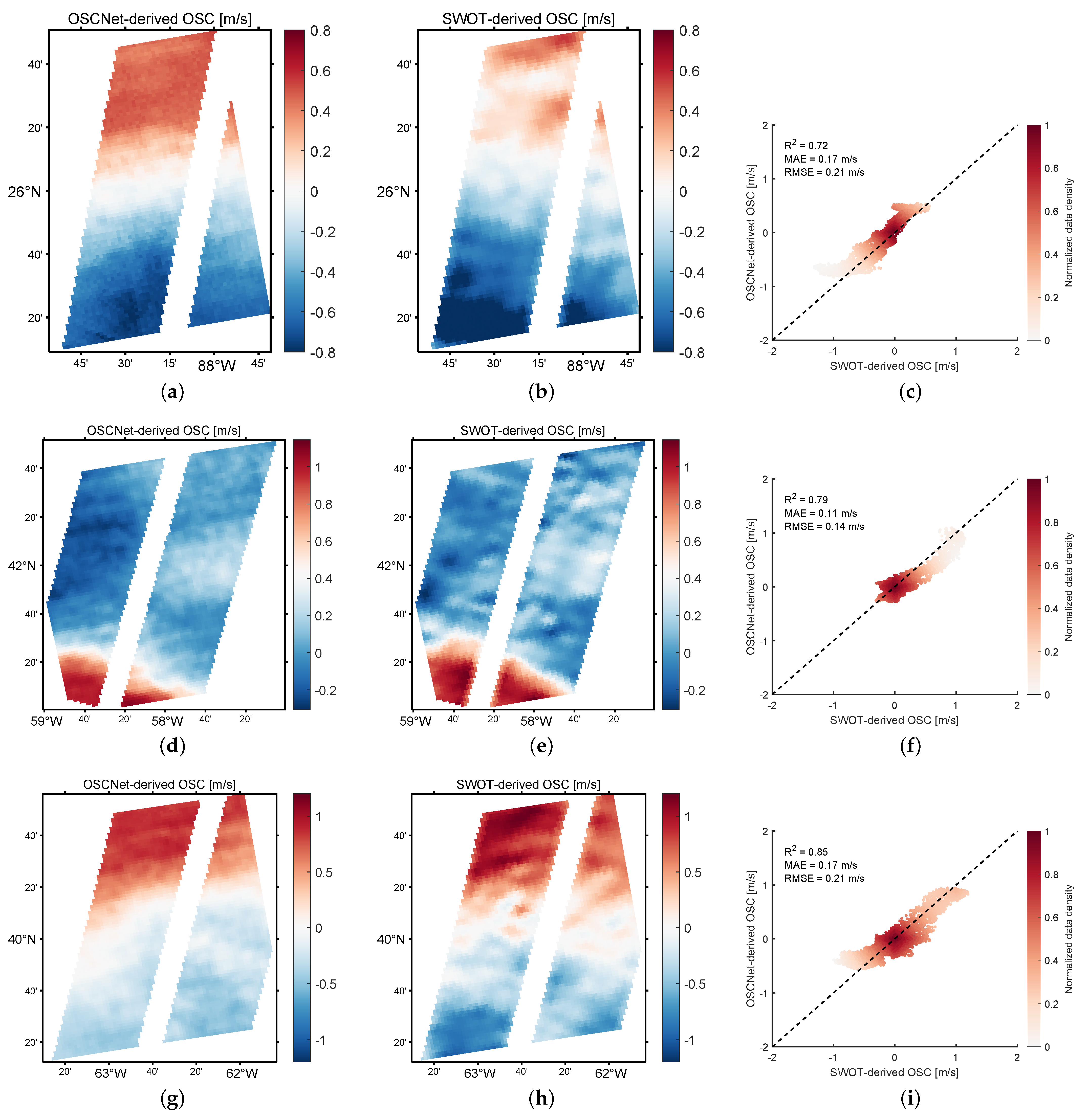
4.1. OSC Retrieval Results

In this study, we utilized S1 and SWOT data from July 2023 to September 2024, yielding approximately 100,819 matchups for the training, validation, and testing of the OSCNet model. The proposed model was evaluated using the metrics outlined in Section 3, where the $R^2$, MAE, and RMSE reached 0.81, 0.15 m/s, and 0.19 m/s, respectively (see

Table 2. Evaluation indicators of different input parameters and models.

Model	Input Parameters							Evaluation Metrics
	Radial Velocity	Wind	Stokes Drift	Wind Wave	Swell	Mean Wave	NRCS	${\mathit{R}}^{\mathbf{2}}$	MAE (m/s)	RMSE (m/s)
OSCNet	✓	✓						0.75	0.18	0.23
	✓	✓	✓					0.78	0.17	0.21
	✓	✓	✓	✓				0.79	0.17	0.21
	✓	✓	✓	✓	✓			0.79	0.16	0.20
	✓	✓	✓	✓	✓	✓		0.80	0.16	0.20
	✓	✓	✓	✓	✓	✓	✓	0.81	0.15	0.19
OSCNet w/o ResNet	✓	✓	✓	✓	✓	✓	✓	0.73	0.18	0.24
CDOP		✓						0.43	0.62	0.69

). To visualize the results, three examples were randomly selected, as shown in Figure 4. Figure 4a,d,g show the radial velocity of the OSC retrieved by the proposed model OSCNet, and Figure 4b,e,h display the OSC derived from SWOT data projected onto the S1 SAR radial direction. Figure 4c,f,i present a comparison between the OSCNet-derived OSC and the SWOT-derived OSC. It can be observed that the OSCNet-derived OSCs are highly consistent with the SWOT-derived OSCs, with the optimal RMSE being 0.14 m/s.

4.2. Ablation Study

In this study, we conducted an ablation study to investigate the impact of input parameters and the incorporation of ResNet on model performance. The performance of models was evaluated using the metrics outlined in Section 3.

4.2.1. Evaluating the Impact of Input Parameters

We trained six models with different input parameter configurations, as detailed in Table 2. The results indicate that the model performs least effectively when the input consists solely of radial velocity and sea surface wind. The optimal model performance is achieved when all seven parameters are incorporated as inputs. It is worth noting that two significant improvements in model performance can be observed: One occurs with the incorporation of swell parameters, and the other occurs with the inclusion of the NRCS. The former is because the incorporation of swell information enables the model to account for the influence of long-period waves on OSC velocity, particularly in regions where wave–current interactions are pronounced, which contributes to a reduction in errors in Doppler centroid estimates caused by sea states. The latter is because the inclusion of the NRCS further enhances the model’s ability to capture the interactions between wind, waves, and currents, especially in cases involving non-uniform scattering, such as variations in sea surface wind speed or the occurrence of wave breaking events.

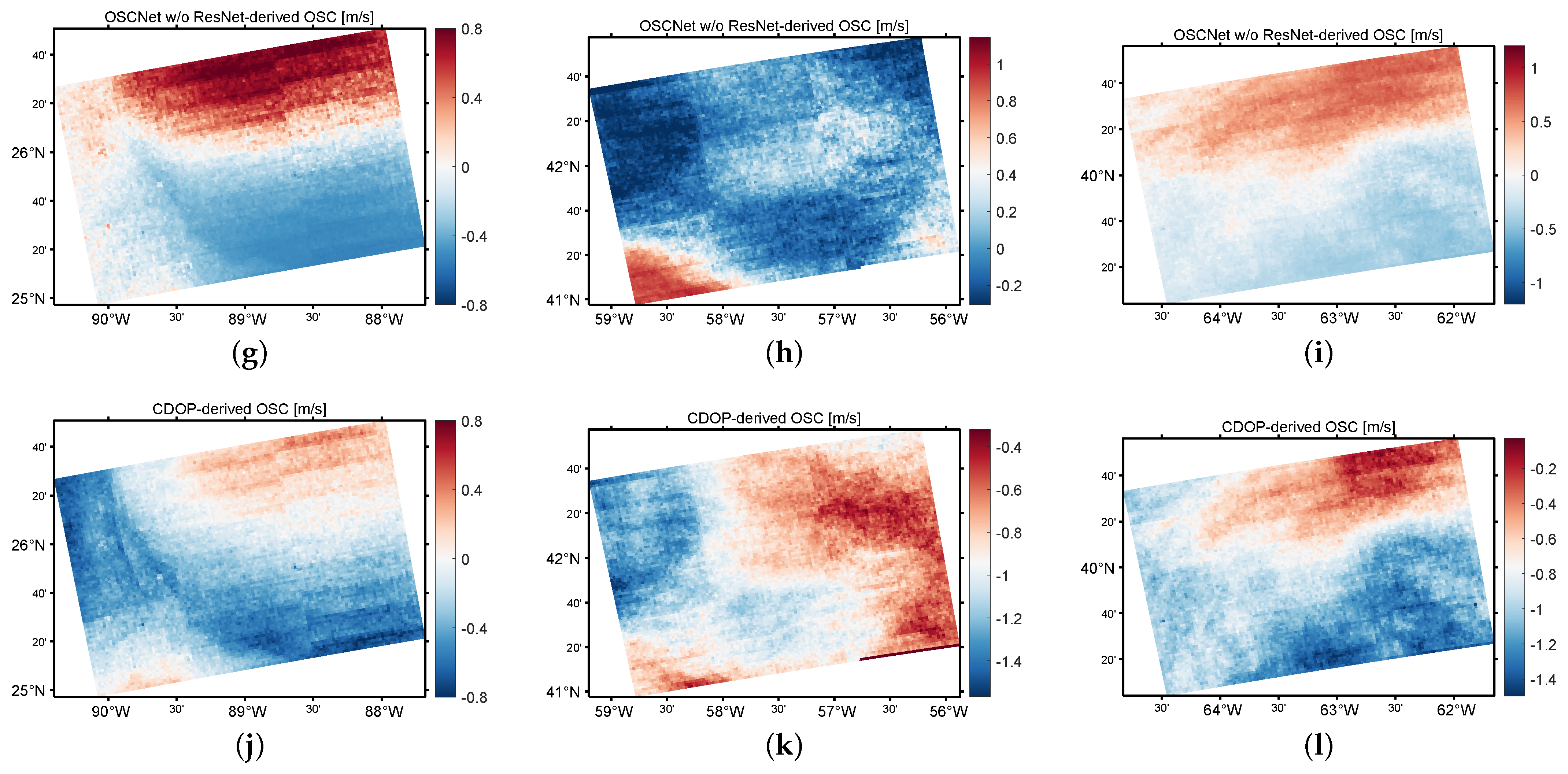
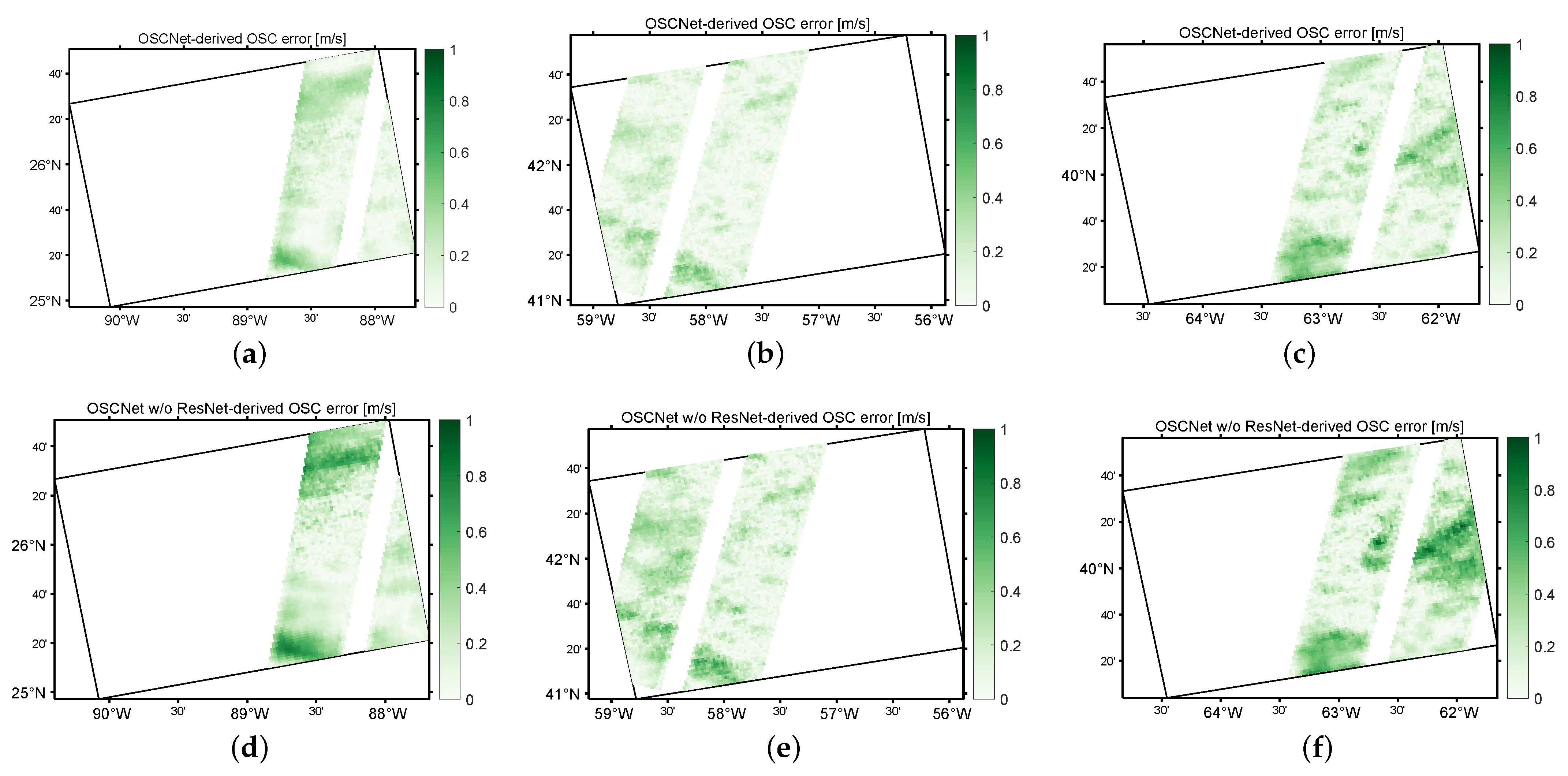
4.2.2. Evaluating the Impact of ResNet

We evaluated the impact of ResNet architecture on model performance while maintaining the model’s input parameters at their optimal configuration. As shown in Figure 5d–i, the OSC retrieval results of the OSCNet model with the ResNet structure closely align with the ground truth, whereas the OSCNet model without the ResNet structure exhibits larger deviations. These discrepancies become more pronounced in regions with higher OSC velocities (see Figure 6a–f). The model’s performance across the entire test dataset is presented in Table 2. As can be seen, the exclusion of the ResNet structure from OSCNet (see “OSCNet w/o ResNet” in Table 2) results in a decrease in $R^2$, along with an increase in MAE and RMSE, compared to the OSCNet model incorporating ResNet. These results indicate the positive influence of incorporating ResNet architecture in enhancing the performance of the OSCNet model in OSC retrieval.

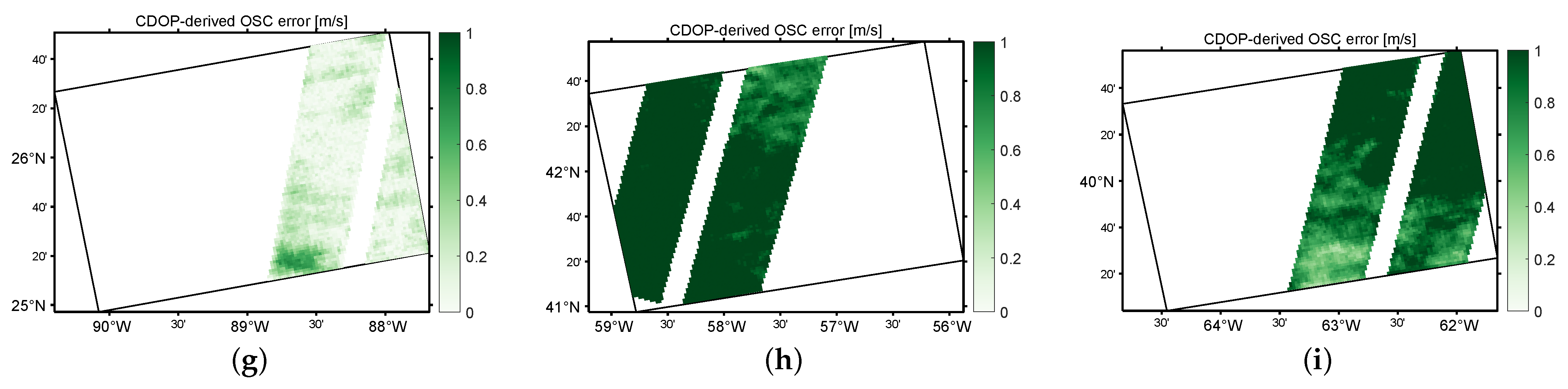
4.3. Model Comparison

To further validate the performance of the OSCNet model, we conducted a comparative experiment between OSCNet and the CDOP model. The CDOP model, developed using a three-layer neural network, is designed to estimate the Doppler shift induced by sea surface winds. Subsequently, the OSC can be obtained based on the assumption that the wind and currents are linearly separable.

Figure 5d–f and Figure 5j–l show the OSC retrieved using the OSCNet and CDOP models, respectively. It can be observed that the OSC retrieved using the OSCNet model closely matches the SWOT-derived OSC, while the OSC retrieved using the CDOP model exhibits significant differences from that retrieved from SWOT data. Figure 6a–c and Figure 6g–i present a quantitative and visual comparison of the retrieval errors between the two models. As can be seen, the OSCNet-retrieved OSC shows higher consistency with the SWOT-derived OSC compared to that retrieved using CDOP model. This discrepancy can be attributed to the fact that the CDOP model fails to account for wave–current interactions, resulting in an overestimation of wind-driven components in regions characterized by strong currents. A performance comparison between the OSCNet and CDOP models across the entire test dataset is summarized in Table 2. It is clear that, compared to the CDOP model, the OSC retrieved using OSCNet exhibits a higher $R^2$, along with a lower MAE and RMSE. These results demonstrate the superior performance of the proposed OSCNet model in OSC retrieval.

4.4. Case Studies

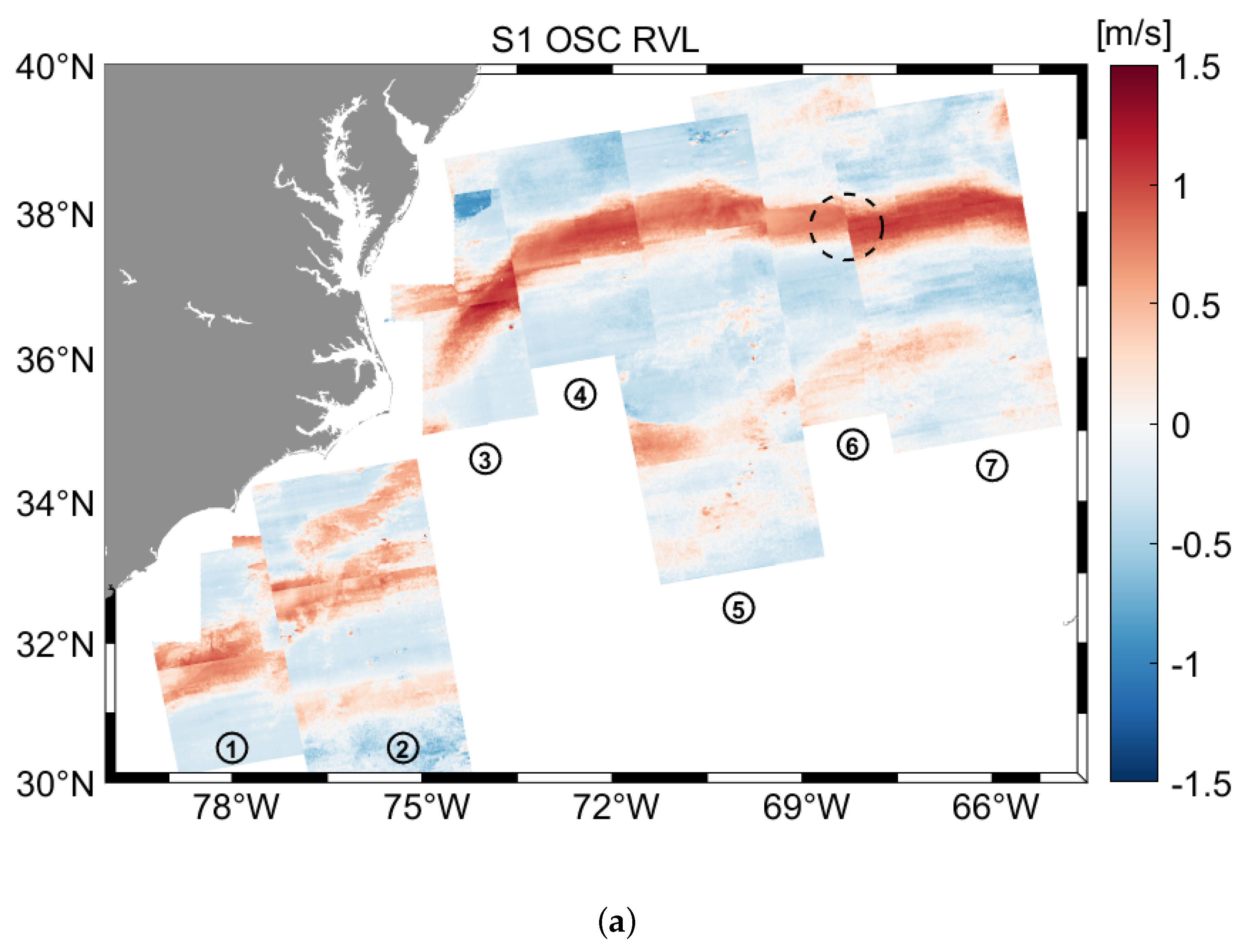
4.4.1. Retrieval of the Gulf Stream Using OSCNet

Figure 7 presents the large-scale OSC retrieval results of the Gulf Stream using the proposed OSCNet model. Figure 7a displays the radial velocity components of OSC derived using OSCNet from seven S1 SAR scenes (numbered 1 to 7) acquired on 12, 19, 26, 9, 16, 11, and 18 August 2023, respectively. Figure 7b shows the Hybrid Coordinate Ocean Model (HYCOM)-simulated OSCs, averaged over the same times as the seven-track SAR data acquisition times. The OSCNet-derived OSC RVL and the HYCOM-simulated OSC exhibit a high degree of consistency in terms of OSC direction, particularly where the Gulf Stream’s primary flow aligns with the S1 SAR radial direction. Although the Gulf Stream deviates from the SAR radial direction in Track 3, the current’s intensity remains sufficiently strong to produce detectable radial velocity components, enabling effective OSC characterization. It is worth noting that a discontinuity in the OSC is observed at the boundary between tracks 6 and 7 (indicated by the black dashed circle in Figure 7a). This discontinuity is mainly caused by two factors: First, the OSC between adjacent SAR scenes is not temporally correlated due to the 7-day time interval; second, the local change in the direction of the Gulf Stream (shown by the red dashed circle in Figure 7b) further exacerbates the OSC RVL misalignment. To mitigate the impact of temporal mismatches, several strategies can be employed. One approach involves the assimilation of complementary data sources, including numerical ocean model outputs, HF radar observations, and satellite altimetry measurements, to provide continuous temporal coverage between SAR acquisitions. An alternative strategy is the use of time-series models, such as recurrent neural networks (RNNs) or long short-term memory (LSTM) networks, which are capable of capturing the temporal dynamics of ocean currents and accounting for their evolution over time.

Figure 8a,b present the OSCNet-derived OSC RVL (from the 16 August 2023 acquisition) and the collocated HYCOM simulations at the nearest available time, respectively. Figure 8c shows a comparison along the transect marked by the black dashed line in Figure 8a,b, revealing a high degree of agreement. In order to quantitatively evaluate the Gulf Stream retrieved by our proposed method, we performed the spatiotemporal matching of the S1 data with HYCOM model data and removed points with low correlations. The quantitative evaluation results are shown in

Table 3. Comparison between the OSCNet-retrieved OSC RVL and HYCOM-simulated OSC RVL.

No.	Acquisition Time	BIAS (m/s)	MAE (m/s)	RMSE (m/s)
1	12 August 2023	−0.18	0.26	0.29
2	19 August 2023	−0.08	0.21	0.26
3	26 August 2023	0.11	0.22	0.25
4	9 August 2023	−0.22	0.26	0.29
5	16 August 2023	0.14	0.22	0.26
6	11 August 2023	0.01	0.23	0.27
7	18 August 2023	−0.21	0.24	0.28

. It can be seen that the optimal MAE and RMSE are 0.21 m/s and 0.25 m/s, respectively. This result not only verifies the reliability of the proposed method but also demonstrates its applicability in strong current retrieval.

4.4.2. Mesoscale Eddies in OSCNet-Retrieved OSC RVL

Figure 9a shows the geographic locations of the co-located S1 and SWOT satellite data, acquired at 22:00:48 UTC and 15:18:51 UTC on 27 August 2023, respectively. The OSCNet-based retrieval documents a structure with OSC RVL $u_{rvl}>0$ and $u_{rvl}<0$ along the azimuth direction (denoted by the red dashed circle in Figure 9b), suggesting the presence of a cyclonic mesoscale eddy. Consistently, the SWOT-retrieved sea surface height anomaly (black dashed circle in Figure 9c) and geostrophic current (red dashed circle in Figure 9d) also reveal the presence of this cyclonic mesoscale eddy. Furthermore, the cyclonic mesoscale eddies detected in the HYCOM-simulated OSC at 21:00:00 UTC on 27 August 2023 (red dashed circle in Figure 9e) and in the sea surface chlorophyll-a observed by the JPSS1 VIIRS at 16:06:00 UTC on the same day (red dashed circle in Figure 9f) both support the OSCNet-based detection of the cyclonic mesoscale eddy.

Figure 10a presents the S1-derived OSC RVL within the red dashed circle in Figure 9b. Figure 10b,c display the projections of the SWOT-derived OSC (Figure 9d) and HYCOM-simulated OSC (Figure 9e) onto the S1 SAR radial direction, respectively. Figure 10d compares the S1-derived OSC RVL, SWOT-derived OSC RVL, and HYCOM-simulated OSC RVL along the black dashed lines in Figure 10a–c, demonstrating strong agreement among them. A quantitative comparison between the OSCNet-derived OSC RVL (Figure 10a) and the SWOT-derived OSC RVL (Figure 10b) is shown in Figure 10e, yielding an $R^2$ of 0.68, a bias of −0.06 m/s, and an MAE of 0.21 m/s. This case study confirms that the proposed method has the capability of detecting mesoscale eddy currents.

5. Discussion

The total velocity of the sea surface measured by SAR primarily consists of two components: wind-driven and non-wind-driven components. The wind-driven component includes Ekman transport, Stokes drift, and the motion induced by wind waves. The non-wind-driven component includes geostrophic currents, tidal currents, and inertial oscillations. The non-wind-driven component is induced by forces independent of the local wind and is the focus of OSC retrieval.

In the case of strong western boundary currents such as the Gulf Stream, the OSC is predominantly governed by geostrophic dynamics, making SWOT-derived geostrophic currents a reasonable reference for validation. However, when extending the model to weaker current regimes, careful attention must be given to non-geostrophic processes such as tides, inertial oscillations, and wind-driven components. Addressing these processes may require adjustments to the model. One promising approach to enhance generalization is transfer learning, where the model trained on the Gulf Stream can be fine-tuned with a smaller amount of data from other regions with varying oceanographic conditions, such as coastal zones. This method allows the model to retain learned features from the primary training dataset while adapting to the specific characteristics of new regions. To further enhance model generalization capabilities, future work will also incorporate data under different sea states. For instance, the inclusion of observations from extreme weather events and calm periods would improve the model’s ability to characterize current dynamics across varying oceanic conditions.

While the necessary resampling and interpolation procedures could potentially introduce artifacts in high-gradient regions, several factors mitigate these concerns. The resampling methods employed are standard practices for aligning datasets with varying resolutions, and the final grid was carefully selected to ensure consistency across all input data. Additionally, although resampling may smooth out some fine details, the model’s overall performance is more strongly influenced by the quality and alignment of the input features, as well as the model’s capacity to handle these processed datasets. Future improvements could explore adaptive interpolation methods or resolution-aware network architectures to optimize spatial fidelity further.

A key limitation of the proposed model is its limitation to radial velocity measurements due to the inherent imaging geometry of SAR. Full current vectors can only be retrieved if the SAR line of sight aligns perfectly with the flow direction. Although SWOT provides geostrophic current vectors, reconstructing full surface current vectors requires accounting for complex sea surface processes (e.g., wind–wave interactions). Future research should focus on integrating SWOT data with complementary remote sensing technologies and numerical model outputs through advanced data assimilation frameworks. Such integration could enable the reconstruction of horizontal current vectors. Furthermore, the development of multi-beam SAR satellites and multi-angle observation techniques is expected to enable more comprehensive measurements of full horizontal current vectors, facilitating the direct retrieval of directional current components through synergistic multi-perspective observations.

6. Conclusions

A reliable OSC estimate from SAR data is challenging to obtain, largely due to difficulties in accurately partitioning the Doppler shifts induced by waves and currents. Recent research on SAR-based OSC retrieval typically assumes that the Doppler shifts caused by wind waves and currents can be linearly superimposed. However, this assumption often leads to large errors in regions characterized by significant nonlinear wave–current interactions.

In this paper, we present a novel deep learning model named OSCNet for OSC retrieval. The model integrates multi-source data, including S1 OCN observations, ECMWF wave parameters, and SWOT Level 3 geostrophic current fields from July 2023 to September 2024. Unlike conventional methods that assume a linear separation of wind and currents, the proposed model utilizes a neural network to directly learn the nonlinear coupling among wind, waves, and currents. By refining physical input parameters, integrating a ResNet architecture, and incorporating NRCS to account for wave breaking and radar backscatter effects, OSCNet achieves an MAE of 0.15 m/s and an RMSE of 0.19 m/s when evaluated against SWOT-derived OSCs. Two case studies further demonstrated that the proposed model is not only capable of retrieving strong currents but also capable of capturing mesoscale eddy currents.

These results demonstrate that OSCNet significantly enhances the accuracy of SAR-based OSC retrieval, particularly in regions characterized by strong nonlinear wave–current interactions. This advancement provides a more reliable approach for ocean surface current monitoring and analysis.

References

1. Villas Bôas, A.B.; Ardhuin, F.; Ayet, A.; Bourassa, M.A.; Brandt, P.; Chapron, B.; Cornuelle, B.D.; Farrar, J.T.; Fewings, M.R.; Fox-Kemper, B.; et al. Integrated Observations of Global Surface Winds, Currents, And Waves: Requirements And Challenges for the Next Decade. Front. Mar. Sci. 2019, 6, 425. [Google Scholar] [CrossRef]
2. Hauser, D.; Abdalla, S.; Ardhuin, F.; Bidlot, J.-R.; Bourassa, M.; Cotton, D.; Gommenginger, C.; Evers-King, H.; Johnsen, H.; Knaff, J. Satellite Remote Sensing of Surface Winds, Waves, And Currents: Where Are We Now? Surv. Geophys. 2023, 44, 1357–1446. [Google Scholar] [CrossRef]
3. Yang, L.; Chen, G.; Zhao, J.; Rytter, N.G.M. Ship Speed Optimization Considering Ocean Currents to Enhance Environmental Sustainability in Maritime Shipping. Sustainability 2020, 12, 3649. [Google Scholar] [CrossRef]
4. Klemas, V. Remote Sensing of Coastal And Ocean Currents: An Overview. J. Coast. Res. 2012, 28, 576. [Google Scholar]
5. Futch, V.; Allen, A. Search And Rescue Applications: On the Need to Improve Ocean Observing Data Systems in Offshore Or Remote Locations. Front. Mar. Sci. 2019, 6, 301. [Google Scholar] [CrossRef]
6. Goldstein, R.M.; Zebker, H. Interferometric Radar Measurement of Ocean Surface Currents. Nature 1987, 328, 707–709. [Google Scholar] [CrossRef]
7. Shuchman, R.; Rufenach, C.; Gonzalez, F.; Klooster, A. The Feasibility of Measurement of Ocean Current Detection Using SAR Data. In Proceedings of the 13th International Symposium on Remote Sensing of Environment, Ann Arbor, MI, USA, 23–27 April 1979; pp. 93–103. [Google Scholar]
8. Romeiser, R.; Runge, H.; Suchandt, S.; Kahle, R.; Rossi, C.; Bell, P.S. Quality Assessment of Surface Current Fields from TerraSAR-X and TanDEM-X Along-Track Interferometry And Doppler Centroid Analysis. IEEE Trans. Geosci. Remote Sens. 2014, 52, 2759–2772. [Google Scholar] [CrossRef]
9. Du, Y.; Shao, J.; Yang, X.; Wang, R.; Yang, J.; Li, X. Investigation of Current-Wave Interaction Effect on Ocean Surface Current Retrieval under DCA Framework Using An Improved Doppler Radar Imaging Model. IEEE Trans. Geosci. Remote Sens. 2024, 62, 4213217. [Google Scholar] [CrossRef]
10. Hansen, M.W.; Collard, F.; Dagestad, K.-F.; Johannessen, J.A.; Fabry, P.; Chapron, B. Retrieval of Sea Surface Range Velocities from ENVISAT ASAR Doppler Centroid Measurements. IEEE Trans. Geosci. Remote Sens. 2011, 49, 3582–3592. [Google Scholar] [CrossRef]
11. Hansen, M.W.; Johannessen, J.; Dagestad, K.-F.; Collard, F.; Chapron, B. Monitoring the Surface Inflow of Atlantic Water to the Norwegian Sea Using ENVISAT ASAR. J. Geophys. Res. 2011, 116, C12008. [Google Scholar] [CrossRef]
12. Rouault, M.J.; Mouche, A.; Collard, F.; Johannessen, J.A.; Chapron, B. Mapping the Agulhas Current from Space: An Assessment of ASAR Surface Current Velocities. J. Geophys. Res. 2010, 115, C10026. [Google Scholar]
13. Fan, S.; Zhang, B.; Kudryavtsev, V.; Perrie, W. Mapping Radial Ocean Surface Currents in the Outer Core of Hurricane Maria from Synthetic Aperture Radar Doppler Measurements. IEEE J. Sel. Top. Appl. Earth Obs. Remote Sens. 2024, 17, 2090–2097. [Google Scholar] [CrossRef]
14. Yang, Z.; Liu, L.; Wang, J.; Miao, H.; Zhang, Q. Extrapolation of Electromagnetic Pointing Error Corrections for Sentinel-1 Doppler Currents from Land Areas to the Open Ocean. Remote Sens. Environ. 2023, 297, 113788. [Google Scholar] [CrossRef]
15. Yang, X.; He, Y. Retrieval of A Real-Time Sea Surface Vector Field from SAR Doppler Centroid: 2. On the Radial Velocity. J. Geophys. Res. 2023, 125, e2022JC019301. [Google Scholar] [CrossRef]
16. Fan, S.; Zhang, B.; Moiseev, A.; Kudryavtsev, V.; Johannessen, J.A.; Chapron, B. On the Use of Dual Co-Polarized Radar Data to Derive A Sea Surface Doppler Model-Part 2: Simulation and Validation. IEEE Trans. Geosci. Remote Sens. 2023, 61, 4202009. [Google Scholar] [CrossRef]
17. Sun, K.; Chong, J.; Diao, L.; Li, Z.; Wei, X. On the Use of Ocean Surface Doppler Velocity for Oceanic Front Extraction from Chinese Gaofen-3 SAR Data. IEEE J. Sel. Top. Appl. Earth Obs. Remote Sens. 2022, 15, 2709–2720. [Google Scholar] [CrossRef]
18. Sun, K.; Diao, L.; Zhao, Y.; Zhao, W.; Xu, Y.; Chong, J. Impact of SAR Azimuth Ambiguities on Doppler Velocity Estimation Performance: Modeling And Analysis. Remote Sens. 2023, 15, 1198. [Google Scholar] [CrossRef]
19. Li, Y.; Chong, J.; Sun, K.; Zhao, Y.; Yang, X. Measuring Ocean Surface Current in the Kuroshio Region Using Gaofen-3 SAR Data. Appl. Sci. 2021, 11, 7656. [Google Scholar] [CrossRef]
20. Chapron, B. Direct Measurements of Ocean Surface Velocity from Space: Interpretation And Validation. J. Geophys. Res. 2005, 110, C07008. [Google Scholar] [CrossRef]
21. Moiseev, A.; Johnsen, H.; Johannessen, J.A.; Collard, F.; Guitton, G. On Removal of Sea State Contribution to Sentinel-1 Doppler Shift for Retrieving Reliable Ocean Surface Current. J. Geophys. Res. 2020, 125, e2020JC016288. [Google Scholar] [CrossRef]
22. Mouche, A.A.; Collard, F.; Chapron, B.; Dagestad, K.-F.; Guitton, G.; Johannessen, J.A.; Kerbaol, V.; Hansen, M.W. On the Use of Doppler Shift for Sea Surface Wind Retrieval from SAR. IEEE Trans. Geosci. Remote Sens. 2012, 50, 2901–2909. [Google Scholar] [CrossRef]
23. Moiseev, A.; Johannessen, J.A.; Johnsen, H. Towards Retrieving Reliable Ocean Surface Currents in the Coastal Zone from the Sentinel-1 Doppler Shift Observations. J. Geophys. Res. 2022, 127, e2021JC018201. [Google Scholar] [CrossRef]
24. Ardhuin, F.; Gille, S.T.; Menemenlis, D.; Rocha, C.B.; Rascle, N.; Chapron, B.; Gula, J.; Molemaker, J. Small-Scale Open Ocean Currents Have Large Effects on Wind Wave Heights. J. Geophys. Res. 2017, 122, 4500–4517. [Google Scholar] [CrossRef]
25. Kudryavtsev, V.; Yurovskaya, M.; Chapron, B.; Collard, F.; Donlon, C. Sun Glitter Imagery of Surface Waves. Part 2: Waves Transformation on Ocean Currents. J. Geophys. Res. 2017, 122, 1384–1399. [Google Scholar] [CrossRef]
26. Wang, H.; Li, X. DeepBlue: Advanced Convolutional Neural Network Applications for Ocean Remote Sensing. IEEE Trans. Geosci. Remote Sens. 2024, 12, 138–161. [Google Scholar] [CrossRef]
27. Ristea, N.-C.; Anghel, A.; Datcu, M.; Chapron, B. Guided Unsupervised Learning by Subaperture Decomposition for Ocean SAR Image Retrieval. IEEE Trans. Geosci. Remote Sens. 2023, 61, 5207111. [Google Scholar] [CrossRef]
28. Zi, N.; Li, X.-M.; Gade, M.; Fu, H.; Min, S. Ocean Eddy Detection Based on YOLO Deep Learning Algorithm by Synthetic Aperture Radar Data. Remote Sens. Environ. 2024, 307, 114139. [Google Scholar] [CrossRef]
29. Zhang, S.; Li, X.; Zhang, X. Internal Wave Signature Extraction from SAR and Optical Satellite Imagery Based on Deep Learning. IEEE Trans. Geosci. Remote Sens. 2023, 61, 4203216. [Google Scholar] [CrossRef]
30. Zhang, X.; Wang, H.; Wang, S.; Liu, Y.; Yu, W.; Wang, J.; Xu, Q.; Li, X. Oceanic Internal Wave Amplitude Retrieval from Satellite Images Based on a Data-Driven Transfer Learning Model. Remote Sens. Environ. 2022, 272, 112940. [Google Scholar] [CrossRef]
31. Wu, K.; Li, X.-M. Deep Learning for Retrieving Omni-Directional Ocean Wave Spectra from Spaceborne Synthetic Aperture Radar. Remote Sens. Environ. 2024, 314, 114386. [Google Scholar] [CrossRef]
32. Zhou, Y.; Shao, W.; Nunziata, F.; Wang, W.; Li, C. An Algorithm to Retrieve Range Ocean Current Speed under Tropical Cyclone Conditions from Sentinel-1 Synthetic Aperture Radar Measurements Based on XGBoost. Remote Sens. 2024, 16, 3271. [Google Scholar] [CrossRef]
33. Yang, Z.; Wang, J.; Liu, L.; Miao, H.; Miao, X.; Zhang, Q. Estimating Effects of Wind And Waves on the Doppler Centroid Frequency Shift for the SAR Retrieval of Ocean Currents. Remote Sens. Environ. 2024, 311, 114312. [Google Scholar] [CrossRef]
34. Shao, W.; Zhou, Y.; Hu, Y.; Li, Y.; Zhou, Y.; Zhang, Q. Range Current Retrieval from Sentinel-1 SAR Ocean Product Based on Deep Learning. Remote Sens. Lett. 2024, 15, 145–156. [Google Scholar] [CrossRef]
35. Bai, Y.; Zhang, Y.; Zhang, X.; Li, X. A Machine-Learning-Based Ocean-Current Velocity Inversion Model Using OCN from Sentinel-1 Observations. IEEE J. Sel. Top. Appl. Earth Obs. Remote Sens. 2025, 18, 9622–9635. [Google Scholar] [CrossRef]
36. Morrow, R.; Fu, L.-L.; Ardhuin, F.; Benkiran, M.; Chapron, B.; Cosme, E.; d’Ovidio, F.; Farrar, J.T.; Gille, S.T.; Lapeyre, G.; et al. Global Observations of Fine-Scale Ocean Surface Topography with the Surface Water And Ocean Topography (SWOT) Mission. Front. Mar. Sci. 2019, 6, 232. [Google Scholar] [CrossRef]
37. Peral, E.; Esteban-Fernández, D.; Rodríguez, E.; McWatters, D.; De Bleser, J.-W.; Ahmed, R.; Chen, A.C.; Slimko, E.; Somawardhana, R.; Knarr, K.; et al. KARIN, the Ka-Band Radar Interferometer of the SWOT Mission: Design and In-Flight Performance. IEEE Trans. Geosci. Remote Sens. 2024, 62, 5214127. [Google Scholar] [CrossRef]
38. Barcelô-Llull, B.; Pascual, A.; Sánchez-Román, A.; Cutolo, E.; d’Ovidio, F.; Fifani, G.; Ser-Giacomi, E.; Ruiz, S.; Mason, E.; Cyr, F. Fine-Scale Ocean Currents Derived from in Situ Observations in Anticipation of the Upcoming SWOT Altimetric Mission. Front. Mar. Sci. 2021, 8, 679844. [Google Scholar] [CrossRef]
39. Holthuijsen, L.; Tolman, H. Effects of the Gulf Stream on Ocean Waves. J. Geophys. Res. 1991, 96, 12755–12771. [Google Scholar] [CrossRef]
40. Hayes, J.G. Ocean Current Wave Interaction Study. J. Geophys. Res. 1980, 85, 5025–5031. [Google Scholar] [CrossRef]
41. Allahdadi, M.N.; He, R.; Neary, V.S. Impact of the Gulf Stream on Ocean Waves. Deep Sea Res. Part II 2023, 208, 105239. [Google Scholar] [CrossRef]
42. He, K.; Zhang, X.; Ren, S.; Sun, J. Deep residual learning for image recognition. In Proceedings of the 2016 IEEE Conference on Computer Vision and Pattern Recognition (CVPR), Las Vegas, NV, USA, 27–30 June 2016; pp. 770–778. [Google Scholar]
Figure 1. The location of the study area. The black box indicates the locations of the matchups represented by the S1 data frame, and the blue arrow indicates the Gulf Stream.
Remotesensing 17 02133 g001
Figure 2. The framework of the proposed method.
Remotesensing 17 02133 g002
Figure 3. The azimuthal and range filters. (a) The notch filter for azimuthal descalloping. (b) The Savitzky-Golay filter for range detrending, where the blue solid line and yellow solid line represent the range profiles before and after filtering, respectively, and the red solid line represents the filter.
Remotesensing 17 02133 g003
Figure 4. (a,d,g) The radial velocity of the OSC retrieved by the proposed model OSCNet. (b,e,h) The OSC derived from SWOT data projected onto the S1 SAR radial direction. (c,f,i) Comparison between the OSCNet-derived OSC and the SWOT-derived OSC.
Remotesensing 17 02133 g004
Figure 5. (ac) The OSC retrieved from SWOT data, where the solid black box indicates the coverage of S1 data. (df) The OSC retrieval results of the proposed OSCNet model with ResNet and (gi) without ResNet under the optimal input parameter configuration. (jl) The OSC retrieval results of the CDOP model. Note that the color bar of the CDOP-derived OSC is scaled to the range that can best present its results, which is inconsistent with other results’ color bars.
Remotesensing 17 02133 g005aRemotesensing 17 02133 g005b
Figure 6. Errors in OSC retrieval results for each model shown in Figure 5. (ac) Retrieval errors of the proposed OSCNet with ResNet. (df) Retrieval errors of OSCNet without ResNet. (gi) Retrieval errors of the CDOP model.
Remotesensing 17 02133 g006aRemotesensing 17 02133 g006b
Figure 7. The retrieval results of the Gulf Stream. (a) OSC RVL derived from S1 SAR time-series Doppler observations using the proposed OSCNet. (b) HYCOM-simulated OSCs temporally averaged over the S1 SAR time-series data acquisition period.
Remotesensing 17 02133 g007aRemotesensing 17 02133 g007b
Figure 8. (a) Enlarged view of the OSCNet-derived OSC RVL within the red box in Figure 7b. (b) Enlarged view of the HYCOM-derived OSC RVL within the red box in Figure 7b. (c) Comparison of OSC RVL profiles along the black azimuth-oriented transect marked in Figure 7a,b.
Remotesensing 17 02133 g008aRemotesensing 17 02133 g008b
Figure 9. (a) Geographic locations of the S1 and SWOT data acquired on 27 August 2023 at 22:00:48 UTC and 15:18:51 UTC, respectively. (b) OSC RVL retrieved using the proposed OSCNet model. (c) SWOT-derived sea surface height anomaly. (d) SWOT-derived OSC. (e) HYCOM-simulated OSC. (f) Sea surface chlorophyll-a observed by the JPSS1 VIIRS on 27 August 2023 at 16:06:00 UTC. The dashed circles indicate the areas of the eddy detected in the subplot (b).
Remotesensing 17 02133 g009
Figure 10. (a) OSCNet-derived OSC RVL, (b) SWOT-derived OSC RVL, and (c) HYCOM-simulated OSC RVL within the dashed circles in Figure 9b, d, and e, respectively. (d) Comparison of OSC RVL profiles along the black azimuth-oriented transect marked in subplot (ac). (e) Comparison of the OSCNet-derived OSC RVL and the SWOT-derived OSC RVL.
Remotesensing 17 02133 g010