Canola Yield Estimation Using Remotely Sensed Images and M5P Model Tree Algorithm

Abstract

Northwestern Ontario has a shorter growing season but fertile soil, affordable land, opportunities for agricultural diversification, and a demand for canola production. Canola yield mainly varies with spatial heterogeneity of soil properties, crop parameters, and meteorological conditions; thus, existing yield estimation models must be revised before being adopted in Northwestern Ontario to ensure accuracy. Region-specific canola cultivation guidelines are essential. This study utilized high spatial-resolution images to estimate flower coverage and yield in experimental plots at the Lakehead University Agricultural Research Station, Thunder Bay, Canada. Spectral profiles were created for canola flowers and pods. During the peak flowering period, the reflectance of green and red bands was almost identical, allowing for the successful classification of yellow flower coverage using a recursive partitioning and regression tree algorithm. A notable decrease in reflectance in the RedEdge and NIR bands was observed during the transition from pod maturation to senescence, reflecting physiological changes. Canola yield was estimated using selected vegetation indices derived from images, the percent cover of flowers, and the M5P Model Tree algorithm. Field samples were used to calibrate and validate prediction models. The model’s prediction accuracy was high, with a correlation coefficient (r) of 0.78 and a mean squared error of 7.2 kg/ha compared to field samples. In conclusion, this study provided an important insight into canola growth using remote sensing. In the future, when modelling, it is recommended to consider other variables (soil nutrients and climate) that might affect crop development.

1. Introduction

Canola (Brassica napus L.) is a significant crop in Canada’s agricultural sector, producing approximately 20 million tons and contributing 25% of the country’s agrarian income annually [1]. Although Western Canada, primarily Saskatchewan, Alberta, and Manitoba, dominates national canola production, Ontario has recently increased its acreage and production due to favorable growing conditions and strong demand for canola oil and meal [1]. For example, within the past five years, Ontario produced around 42,487 tons [2]. Additionally, more farmers are incorporating it into crop rotations due to its profitability, role in improving soil health, and the adoption of new technologies [3]. Canola is primarily grown in southern and central Ontario, particularly in counties such as Essex, Chatham-Kent, Lambton, and Huron, where the climate and soil conditions favor its cultivation [1,4]. Although Northwestern Ontario meets favorable conditions for growing canola, research should be conducted to confirm suitable varieties, types of fertilizers, application timings and quantities, and other relevant factors.

The accurate and fast technology of estimating rapeseed yield is significant in sustainable agricultural management [5]. For instance, accurate projections enhance the understanding of production dynamics (revenue planning and budgeting), facilitating informed decision-making regarding import and export policies, resource and risk management, and effective agricultural supply chain planning (food security) [6,7,8]. Traditionally, yield is estimated by hand counting, a simple process for counting seedlings and flowers. However, it is a time-consuming and labor-intensive process that is not feasible for sizeable agricultural production fields [9,10]. In contrast to traditional methods, more efficient and non-invasive practices based on remote sensing technologies are being developed. Time-efficient and cost-effective methods for estimating biomass and assessing crop yield have been analyzed [11]. Furthermore, farmers can optimize inputs such as water, fertilizers, and pesticides by predicting crop yields using precision agriculture and remote sensing technologies. This helps maximize productivity while minimizing costs and environmental impact, leading to more sustainable farming practices [12].

The plant is a member of the mustard family and can grow up to 1.5 m tall [5]. It produces small, vibrant yellow flowers that develop into pods that resemble peas and contain tiny black seeds. When canola seed development begins, canola yield is closely tied to the plant’s flowering phase. The flowering period significantly influences grain yield and oil concentration, with the timing and duration of the flowering stage being key determinants of pod formation and crop production [13]. However, weather, soil conditions (including water, nutrient levels, and soil type), deteriorating land quality, crop management practices, and local cultivars—different canola varieties grown in various regions—each have unique weather characteristics that impact yield [7]. Therefore, remote sensing-based canola yield estimation models must be adapted or retrained for each region to ensure accuracy, especially in addressing the spatial heterogeneity of soil properties, crop parameters, and weather [7]. A model trained in one area, such as Saskatchewan, Canada, may not work well in Northwestern Ontario without proper adjustments.

A study conducted in China revealed the number of oilseed rape flowers by combining vegetation indices (VI) and image classification (multispectral images from blue, green and red (RGB) regions) [14]. Nguyen et al. [15] demonstrated that medium-resolution multispectral satellite imagery (Sentinel-2), combined with simple empirical models, can accurately assess canola crop yield over large areas. Tian et al. [16] developed a new canola flower index (CFI) based on Sentinel-2 image bands (red, green, blue, and near-infrared) to improve canola flower classification. This approach achieved an overall accuracy of 96% and a kappa coefficient of 0.91 using a decision tree model and the Google Earth Engine (GEE). Their study demonstrated the effectiveness of the CFI-based model in accurately identifying canola flowers [16]. Due to the large area of interest, the medium spatial resolution of the satellite images did not hinder the information extraction process. However, a few studies used multispectral images from Unmanned Aerial Vehicles (UAVs) to analyze canola at higher spatial resolution. Zhang et al. [17] indicated the Normalized Difference Yellowness Index (NDYI) derived from UAV images as a useful vegetation index for analyzing canola flowering pixel numbers and flowering intensity. They also confirmed that NDYI-based flowering pixel numbers are a good predictor of pod numbers and, thus, canola yield (R² up to 0.42). However, this study recommended testing a multivariate model using several vegetation indices to improve the yield estimation accuracy [17].

Several studies examined the physiology and phenology of canola vegetation [18]. Fernando et al. [19] employed linear discriminant analysis (LDA) to evaluate the spectral characteristics of yellow flowers using four spectral indices derived from red, green, and blue bands: Normalized Difference Yellowness Index (NDYI), Modified Yellowness Index (MYI), Red Blue Normalizing Index (RBNI), and High-Resolution Flowering Index (HrFI). MYI, HrFI, and RBNI were new indices developed to quantify pixels corresponding to canola flowers. As a result, crop yield was predicted with 75% accuracy and maximum flowering was confirmed as a positive yield indicator (R² = 0.82) [18]. Lukas et al. [20] tested BNDVI, NDYI, and Normalized Difference Vegetation Index (NDVI) derived from UAV images at the flowering stage to predict the canola yield and identify changes during the flowering phenological period of the crop. Rai et al. [21] employed a total of 27 existing vegetation indices (VIs), including Canola Ratio Index (CRI), Structure Intensive Vegetation Index (SIPI), Canola Index (CI), and Green Normalized Difference Vegetation Index (GNDRE), derived from images acquired using a small UAV as potential predictor variables and four machine learning algorithms to predict canola yield. When using machine learning algorithms to predict yield at the peak flowering and pod-filling stages, the prediction accuracies (R²) were 0.69 and 0.6, respectively. This study identified several limitations and future considerations. One recommendation was to focus on the complex interaction between canola and its environment, including genetics, environmental factors (such as soil and weather), and management practices, in the model. However, this study highlighted the applicability of a combination of small UAV imagery and VIs for yield estimation in commercial farms [21]. Ahmed et al. [22] also utilized NDYI to assess the canola growth stages and predict seed yield. Since the seed yield of canola widely varies by region, year, soil moisture, and growing season precipitation, it is still necessary to conduct regional studies [23]. Further, most studies have emphasized the importance of integrating multiple vegetation indices (multivariate models) to improve the accuracy of canola yield estimation.

Muruganantham et al. [24] reviewed several studies that employed remote sensing images and deep learning algorithms (from 2012 to 2022). The review confirmed that the deep learning algorithm’s performance and accuracy are better than traditional machine learning algorithms for crop yield estimation using multispectral images spanning visible to near-infrared (NIR) regions or beyond. Among those studies, the Long Short-Term Memory (LSTM) and Convolutional Neural Networks (CNN) algorithms are the most widely used deep learning approaches; however, the performance of all models varies with the factors and parameters used [24].

Decision trees are widely used in supervised learning, which divides the attribute space into groups or clusters based on the patterns learned from the data. Each cluster is well-defined, facilitating the assignment of new data to their corresponding group [25]. A variation of the decision tree, known as a model tree, resembles regression trees but differs because the leaves are associated with multivariate models rather than simple labels [25]. This allows the model to capture more complex relationships [25,26]. A well-known example of a model tree is the M5 Model tree developed by Quinlan [27]. Unlike the normal decision tree, the M5 Model tree follows the basic tree model, but each leaf (node) performs a linear regression between the dependent and independent variables [28]. According to Keshtegar [29], this model works based on a decision tree structure to replace linear regression equations at each node, which allows the prediction of numerical variables. The M5P error is determined by the standard deviation of the class values at each node, and this error determines the tree-division criteria at each node. This division creates a large tree structure that might lead to overfitting. However, an extended version of the M5P Model Tree, developed by Witten & Frank [30] includes a pruning step that simplifies the tree by eliminating nodes whose attributes do not contribute to error reduction, thereby reducing the tree size without compromising accuracy. Furthermore, Taghi [31] emphasized that the model is distinguished by its lower computational cost and its ability to combine multiple simple linear relationships efficiently. Therefore, the M5P model’s use of linear equations for predicting target values ensures simplicity in interpretation and computational efficiency, making it an ideal choice for predicting canola crop yield.

Alipour et al. [32] showed that the M5P model can effectively estimate evapotranspiration using climate data from the Moderate Resolution Imaging Spectroradiometer (MODIS), achieving a coefficient of determination (R²) of 0.80. A study conducted by Karthikeyan & Murugan [33] analyzed groundnut and maize in different states of India using various machine learning approaches. The results indicated strong positive correlations for yield prediction and model development. In particular, the M5P model tree was identified as the most effective, with a correlation coefficient of 0.95 and a Root Mean Square Error (RMSE) of 78.66%. Another study by Gonzalez-Sanchez et al. [34] showed that the M5P model has potential for crop yield prediction, with an RMSE of 74.34% and a correlation coefficient (r) of 0.77, using a complete subset of climatic attributes.

This study aimed to analyze the spectral variation of canola phenology over time and estimate canola yield using a time series of remotely sensed images and the M5P Model Tree algorithm. This study employed a multivariate linear model to predict canola yield for the first time, assuming that error minimization techniques at each internal node enhance prediction accuracy and that internal nodes learn efficiently and handle high-dimensional data. The specific objectives were to (1) estimate the spectral profile of canola flowers at their peak growing stage, (2) calculate the percent cover of flowers for each plot, (3) analyze the spectral variation of pods over time, and (4) predict seed yield for each plot.

2. Materials and Methods

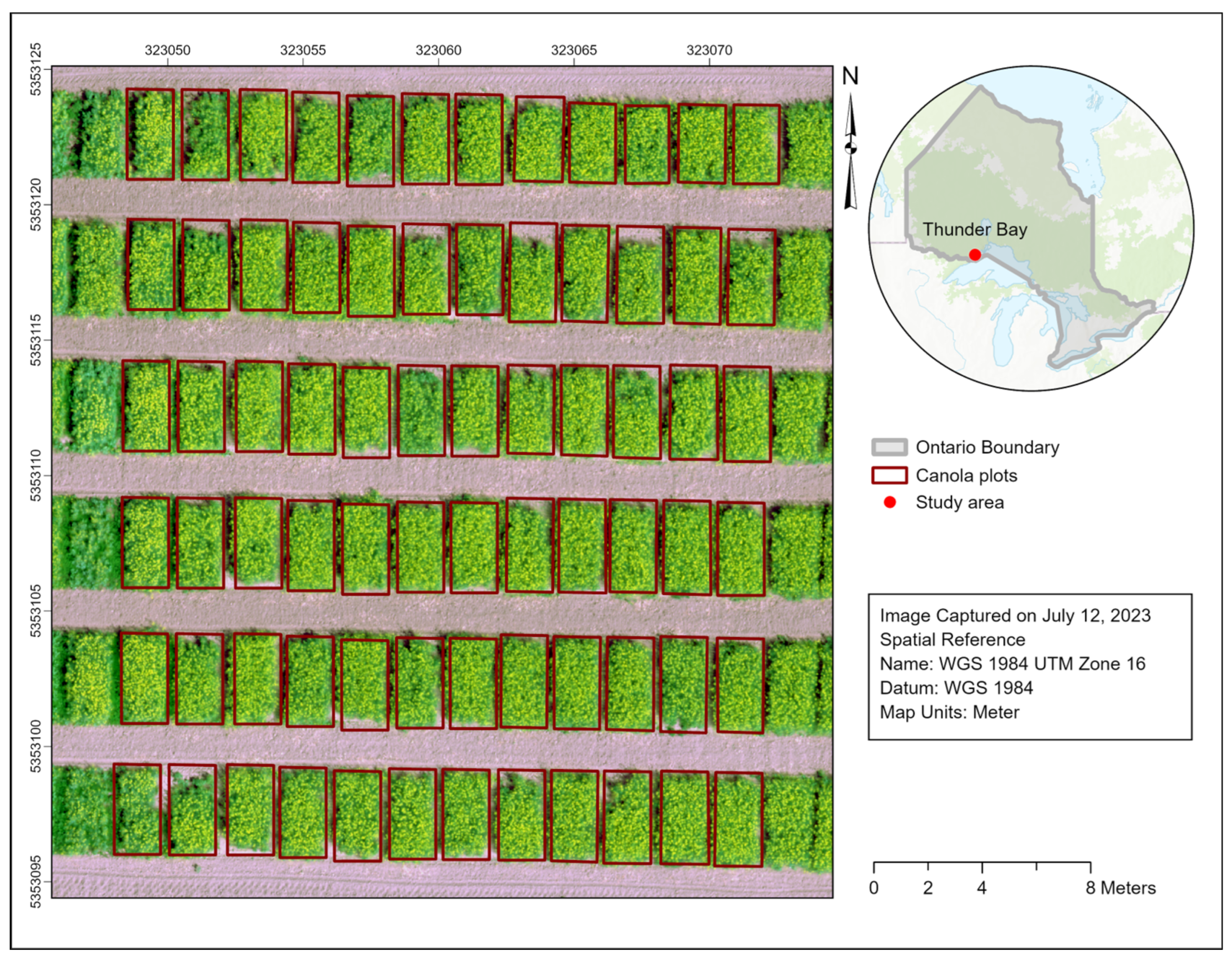
2.1. Study Area and Data

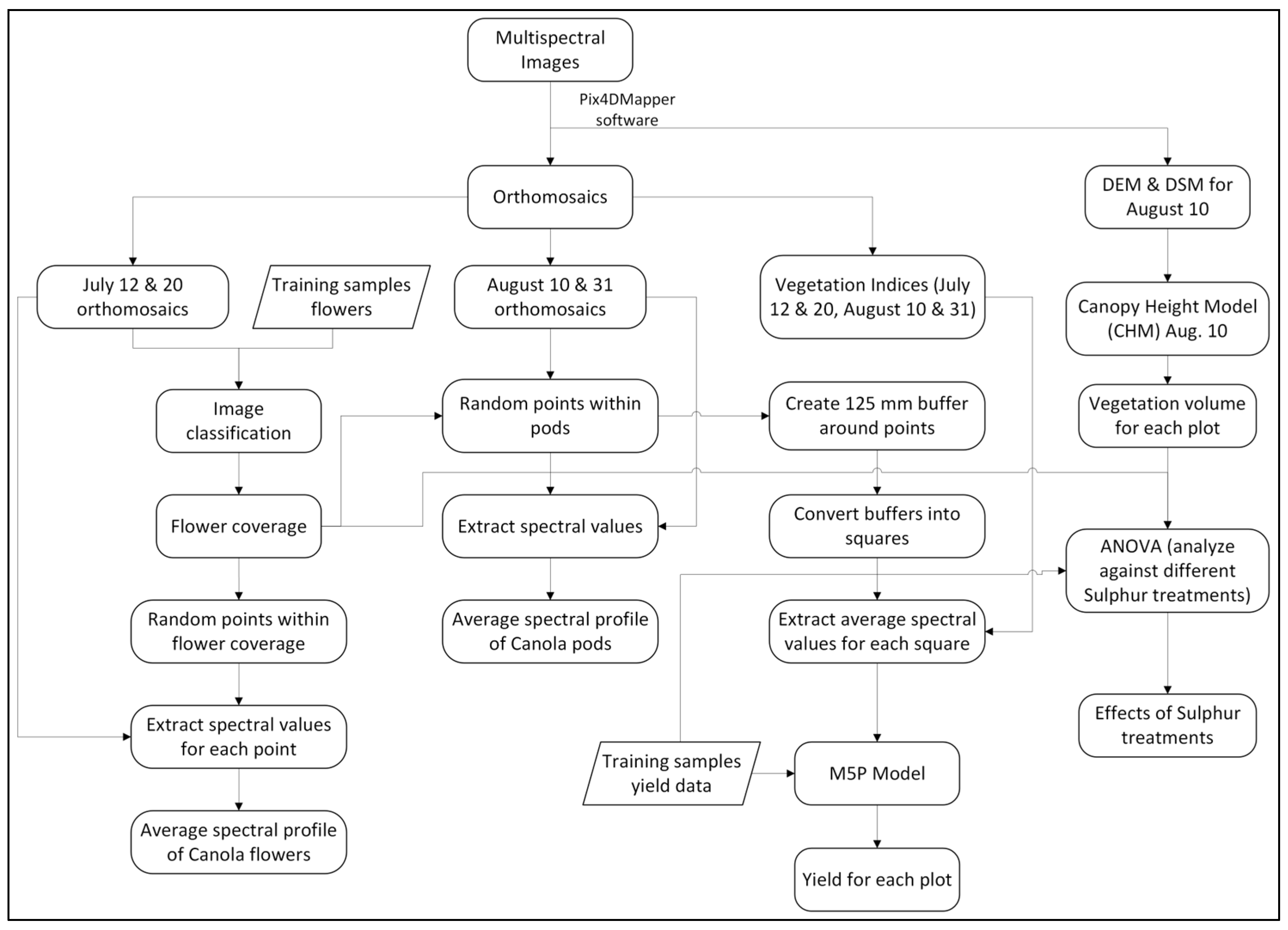
This study was conducted at the Lakehead University Agricultural Research Station (LUARS), located in Thunder Bay, ON, Canada, at the following coordinates: 48°18′23″N, 89°23′11″W. The primary purpose of this research station is to promote and transfer agricultural research for further development and diversification in Northwestern Ontario [35]. LUARS tests new varieties of field crops, different types of fertilizers and pesticides, and the timing of their application to advise farmers in the region. This particular study utilized canola plots, which were treated with sulfur-based fertilizers.

In this study, canola was seeded on 26 May 2023, over 72 experimental plots, each measuring 6 m² (Figure 1). The total area of our study site was approximately 722.40 m². About one-third of the plots were treated with varying sources of Sulfur (S), which were applied before planting at a rate of approximately 36 kg/ha (

Table 1. Different Sulfur treatments for plots.

Treatment No.	Treatment
T1	No Sulfur
T2	Ammonium Sulphate at 36 kg S/ha and Phosphorous as per soil test
T3	Ammonium Sulphate at 36 kg S/ha
T4	Ammonium Sulphate at 24 kg S/ha and SymTRX S10 * at 12 kg S/ha
T5	Ammonium Sulphate at 18 kg S/ha and SymTRX S10 * at 18 kg S/ha
T6	Ammonium Sulphate at 12 kg S/ha and SymTRX S10 * at 24 kg S/ha
T7	SymTRX S10 * at 36 kg S/ha

* SYMTRX S10 (14-24-0-10) is a bio-based fertilizer containing 16% O.M., which could increase microbial activity.

). The effect of fertilization on crop development and yield amount was not evaluated in this study; only the relationship between seed yield, percent cover of flowers, and spectral properties of canola at several stages was analyzed.

Remote sensing images were acquired throughout the growing season, from 12 May to 31 August 2023. The images were captured using a MicaSense Rededge MX camera (MicaSense, Inc., Seattle, WA, USA) [36] mounted on a DJI Matrice-300 drone (DJI, Shenzhen, China) [37]. These images had five multispectral bands (blue, green, red, red edge, and NIR bands), and the spatial resolution was 2 cm (flying height was 30 m above ground level).

The first set of images was taken on 12 May 2023, during the seeding stage. Small plants emerged on 26 May 2023. By 8 June 2023, the plants had approximately four leaves, which were used to map vegetation coverage and assess the success rate of germination of each plot. On 31 August 2023, the middle rows of 28 plots were harvested, and straw and seed yields were measured using the standard yield estimation process.

2.2. Method

In summary, orthomosaics were generated for 12 and 20 July, and 10 and 31 August. The extent of flower coverage was calculated using images from 12 July to 20 July. Random points were generated within the flower coverage, and spectral information was extracted for each point. An average spectral profile for canola flowers was derived (Figure 2). Similarly, spectral information was extracted from canola pods, and their spectral profiles were generated over time. By using a Digital Surface Model (DSM) and a Digital Elevation Model (DEM) from 10 August images, a Canopy Height Model (CHM) was generated, and the vegetation volume for each plot was extracted. Flower percent cover, vegetation volume, and seed yield collected in the field were statistically analyzed to check the similarities due to different treatments (Table 1). Finally, by combining field samples, selected vegetation indices (for the above four dates), and the M5P Model Tree algorithm, the canola yield for each plot was predicted. The accuracy of the model was assessed against the field data. The overall method is explained in Figure 2.

Areial images were corresponded to various stages of canola growth, including leaf development, rosette formation, flowering, pod development, and maturation (

Table 2. Canola growth stages and corresponding image capture dates provide a visual guide to canola development [38].

Stages	Image Date
Bare soil/seeding	12 May 2023
Germination	26 May 2023
Leaf development	8 and 16 June 2023
Rosette	23 June 2023
Bolting	4 July 2023
Flowering	12 July 2023
Podding	20 July 2023
Ripening	10 August 2023
Senescence/harvesting	31 August 2023

) [38]. The multispectral images were processed using Pix4DMapper software (version 4.9) [39], and radiometrically corrected orthomosaics, digital elevation models (DEMs), and digital surface models (DSMs) were generated for 12 and 20 July, and 10 and 31 August.

2.2.1. Spectral Profile of Canola Flowers

The flower coverage of our study area was isolated by classifying two orthomosaics (12 and 20 July 2023), which represented the peak flowering dates. Based on the visual appearance of those images, seven classes were identified for 12 July (two classes of flowers (very bright yellow and light yellow), two classes of vegetation (canola and other), two classes of shades/shadows, and soil). For 20 July, four classes were identified (flowers, pods, soil, and shadows). The training samples (points) were prepared manually (998 points). Special attention was given to assigning approximately equal points for each class. A recursive partitioning and regression tree algorithm was used to classify the images from the “rpart” package [40] in R software (version 4.4.2). The decision tree algorithm is a machine learning method that utilizes a hierarchical structure to divide data into multiple stages, making it suitable for both classification and regression tasks [41]. This method consists of a root node, internal nodes, and leaf nodes, with each node applying binary decisions to separate classes based on a top-down induction methodology [41,42]. Once the classification was completed, the flower coverage within each field plot was extracted. The accuracy of classified flower classes was assessed using a confusion matrix. The user’s and producer’s accuracy of flower classes were noted.

Random points (2000) were generated within the flower coverage, and their spectral values were extracted. The spectral profile for each point, and thus, the average profile of the flowers, was generated (Figure 2). The percentage of flower coverage was evaluated at the pixel level. The percentage of flower area in each plot was calculated based on the classification results and the extent of each plot (Equation (1)). An exploratory data analysis (EDA) was performed for each plot’s percentage of flower coverage (box plots, histograms, and QQ plots) to analyze the variations among them.

$$\mathrm{Percentage} \mathrm{of} \mathrm{Flower} \mathrm{Coverage} \mathrm{for} \mathrm{each} \mathrm{plot} \left(\%\right)={\displaystyle \frac{\mathrm{Flower} \mathrm{extent} \mathrm{of} \mathrm{each} \mathrm{plot} \left({\mathrm{m}}^2\right)}{\mathrm{Individual} \mathrm{plot} \mathrm{extent} \left({\mathrm{m}}^2\right)}} \times 100$$

(1)

2.2.2. Estimating Canola Yield Using Remote Sensing

Within our study area, the two middle rows of each plot (28 plots in total) were harvested, and the seed yield per plot was calculated. These values were used as calibration and validation data for yield prediction. Random points (1000) were generated within the flower coverage area of the above plots. These points were manually cleaned by overlaying the August 10th image (at the ripening stage) and verifying if they fell within the pod areas. If points were outside the pod areas, they were deleted. Finally, 900 points remained, with 70% used for yield estimation and 30% for accuracy assessment. A 125 mm buffer zone was created for each point, and these buffer circles were converted into squares. The average yield for each square was assigned.

A total of 11 vegetation indices (

Table 3. Vegetation indices used to estimate canola yield.

Vegetation Index	Equation
Normalized Difference Yellowness Index [44]	NDYI = (G − B)/(G + B)
Difference Yellowness Index [44]	DYI = G − B
Canola Index [45]	CI = NIR × (R + G)
Canola Ratio Index [43]	CRI = G/B
Canola Flower Index [16]	CFI = NDVI × (R + G)
Normalized Difference Red Edge [48]	NDRE = (NIR − RE)/(NIR + RE)
Green Normalized Difference Vegetation Index [49]	GNDRE = (RE − G)/(RE + G)
Normalized Difference Vegetation Index [50]	NDVI = (NIR − R)/(NIR + R)
Blue Normalized Difference Vegetation Index [44]	BNDVI = (NIR − B)/(NIR + B)
Structure Insensitive Pigment Index [51]	SIPI = (NIR − R)/(NIR − B)
Normalized Difference Red-Blue Index [52]	NDRB = (R − B)/(R + B)

B = Blue, G = Green, R = Red, RE = Red edge, and NIR = Near Infrared.

) were calculated from the images captured during various growth stages of canola: peak flowering (12 July 2023), beginning of the podding (20 July 2023), ripening (10 August 2023), and senescence (31 August 2023), resulting in 44 vegetation indices. These VIs were selected primarily based on the spectral behavior of flowers and pods observed in this and previous studies. The first five indices in Table 3 were adapted from studies that focused solely on canola [19,43,44,45]. At canola peak flowering, the carotenoids in the yellow flowers absorb blue light and reflect both green and red light. Therefore, indices derived from the green and blue bands are suitable, such as the Normalized Difference Yellowness Index (NDYI) and Difference Yellowness Index (DYI) [46]. Canola Index (CI), Canola Ratio Index (CRI), and Canola Flower Index (CFI) were used by Fernando [46] in her research to quantify the reproductive period of canola and, consequently, estimate the canola seed yield. Furthermore, according to Sulik & Long [43], the CRI correlates with changes in flower density. Similarly, Rai et al. [21] considered the use of the Normalized Difference Red Edge (NDRE) and the Green Normalized Difference Vegetation Index (GNDRE) to estimate potential canola yield. Normalized Difference Vegetation Index (NDVI) indicates the health and vigor of the vegetation and chlorophyll content in the leaves [47]. The Blue Normalized Difference Vegetation Index (BNDVI) functions similarly to NDVI but replaces the red band with the blue band in its calculation [44]. Finally, the Structure Insensitive Pigment Index (SIPI) examines the proportion between chlorophyll and carotenoids [16].

The correlation between seed grain (metric tons per ha (mt/ha)) and previously calculated vegetation indices was analyzed. The indices with the highest correlation (greater than 0.7) on all four dates and the percentage of flower coverage (

Table 4. Selected predictor variables to estimate canola yield *.

Image Date	Vegetation Index
20 July	CI, CRI, CFI, DYI, NDYI, NDVI, SIPI, GNDRE, and NDRB
31 August	CRI, CFI, and NDYI
12 and 20 July	Percentage of flower coverage

* These vegetation indices received the highest correlation with yield (metric tons per ha) for each plot.

) were selected for the M5P Model (predictor variables).

The average VIs for each square were calculated using the “Zonal Statistics as Table” tool in ArcGIS Pro software (version 3.3.0) [53]. An exploratory data analysis (EDA) was performed (box plots, histograms, QQ plots, and scatter plots) to analyze the distribution of these data. After that, outliers were removed, and the normality of the data was checked. Finally, a table with yield estimation and 12 predictor variables (Table 4) was prepared for yield modelling.

Canola yield for each experimental plot was estimated using the M5P Model Tree. The dataset was randomly divided into training (70%) and validation (30%). The RWeka package (version 0.4-46) [54] in the R software (version 4.4.2) [55] was used to predict yield in metric tons per hectare (mt/ha). When constructing the model tree, it first generated regression trees using training data, then simplified the regression trees by first post-pruning, deleting nodes of linear models that didn’t improve the accuracy. Finally, the tree size was reduced without compromising accuracy (second post-pruning) [25]. These nodes had classification errors greater than those of the linear models corresponding to intermediate nodes [25].

First, the model sensitivity was assessed using cross-validation in various ways: Correlation coefficient (r), Mean Absolute Error (MAE), Root Mean Square Error (RMSE), Relative Absolute Error (RAE), and Root Relative Squared Error (RRSE). After that, the model’s prediction performance was assessed using validation data, and the results were noted as r, MSE, and RMSE. Finally, this model was used to predict the spatial distribution of yield over experimental plots. The accuracy of the prediction map was also assessed based on the validation samples.

Although this study did not intend to evaluate the effect of different Sulfur treatments in detail, the One-way (ANOVA) method was used to check whether there are significant differences in flower coverage, vegetation volume, seed yield, and predicted seed yield among different treatments (T1 to T7 in Table 1). Individual data series were tested for normality, and outliers were removed if present before conducting the ANOVA tests.

3. Results

3.1. Spectral Profile of Flowers

Canola flowers were successfully detected. The producer’s accuracy (Prod. Acc.) and user’s accuracy (User Acc.) for both days showed acceptable accuracy levels (

Table 5. The accuracy assessment of canola flower classification.

Image Date	Class *	Producer’s Accuracy	User’s Accuracy
12 July 2023	Flowers 1	84.62%	88.00%
	Flowers 2	91.67%	84.62%
20 July 2023	Flowers 1	100.00%	98.28%

* Canola flowers were divided into two classes (Flowers 1 (bright yellow, fully bloomed) and Flowers 2 (light yellow, partially bloomed)) based on their spectral differences in brightness and color.

). The classification corresponding to 20 July showed the highest accuracy values, with a producer’s accuracy of 100.00% and a user’s accuracy of 98.28%.

The average reflectance values showed a clear trend, with the blue band presenting the lowest value (0.03), followed by an increase in the green band and a slight decrease in the red band (0.11). There was an increase in the RedEdge band (0.30), and finally, the highest value was observed in the NIR band (0.65) (Figure 3). This pattern is slightly different from the spectral profile of healthy vegetation.

The analysis of the percent flower coverage in 72 experimental plots demonstrates that the degree of dispersion of the points appears uniform, indicating no clear trend or clustering among the data, suggesting that the percentage of flower coverage is constant across observations. As shown in the Index plot (Figure 4a), the horizontal axis, labelled “Index,” illustrates how the percentage of flower coverage disperses in the order in which the data were entered. Since they were distributed randomly, it can be concluded that no spatial pattern was exhibited with this data. The histogram showed that the data distribution is mainly concentrated in the 30–35% range. Most plots have approximately 30–35% flower coverage. Some outliers were indicated in the box plots and the Normal Q-Q plot. Once outliers were removed, the data were found to be normally distributed.

There were four plots for each treatment (28 plots in total). The null hypothesis for the ANOVA test on flower percent cover was that there were no significant differences between the treatments; the mean values were similar between T1 and T7. The p-value was greater than the critical value (95% confidence interval), indicating no significant evidence to reject the null hypothesis. Therefore, it can be concluded that there were no significant differences in the percentage of flower coverage among the different treatments. A similar situation was observed regarding vegetation volume, field-measured seed yield, and predicted seed yield.

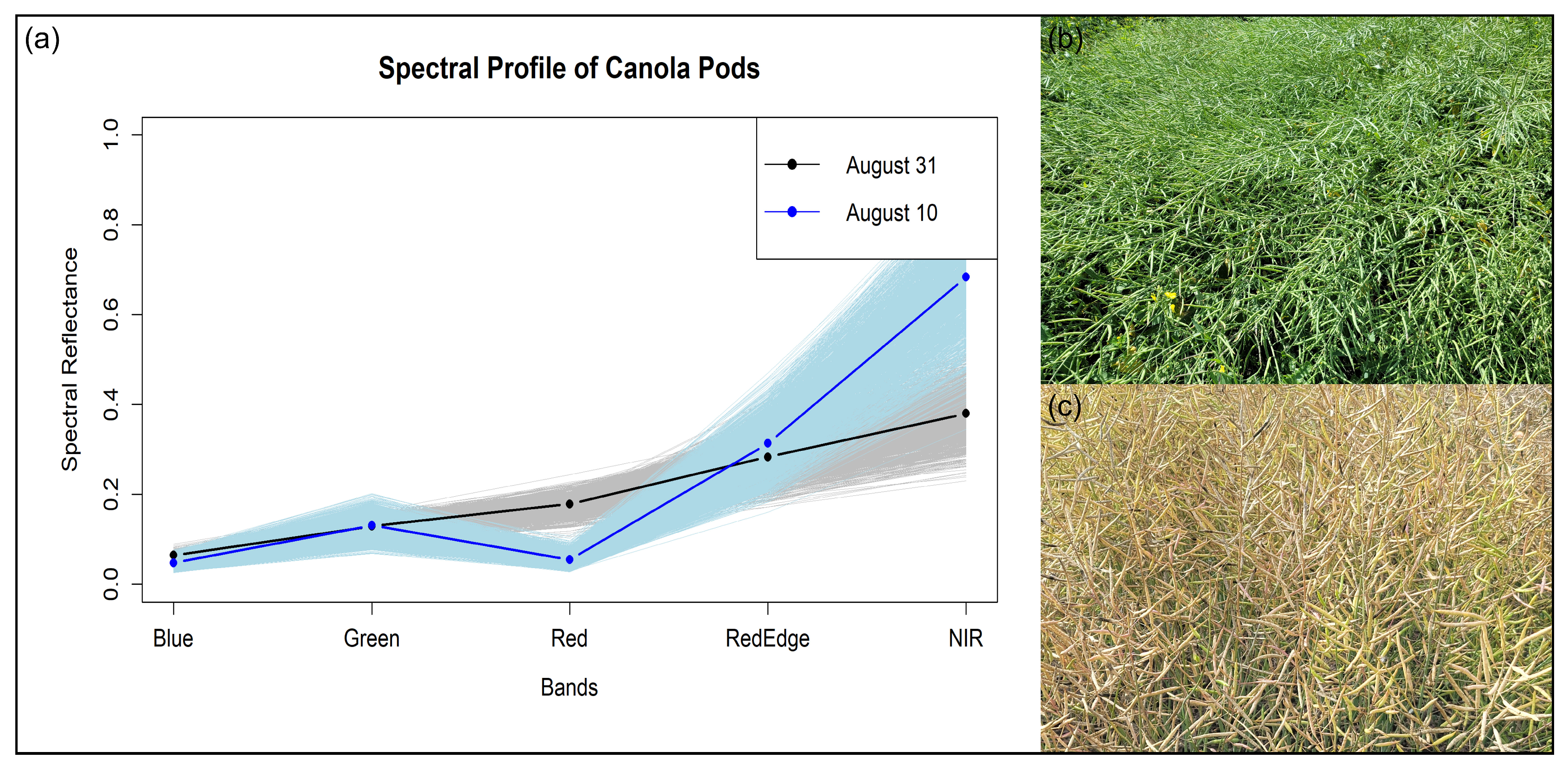
3.2. Spectral Variations of Canola Pods

The spectral profiles of pods during the ripening and senescence stages revealed significant differences, especially in the red and NIR bands. The red reflectance values were slightly higher at the senescence stage, while the NIR band value was considerably lower than the respective values at the ripening stage (Figure 5). This can be attributed to the physiological changes that the pods undergo during their transition to full maturity. In contrast, an increase in reflectance values in the RedEdge and NIR bands was observed at the ripening stage.

3.3. Estimating Canola Yield Using Time Series of Remote Sensing Images

Twelve vegetation indices highly correlated with yield data and the percentage of flower coverage for each plot were selected for yield estimation (Table 4). For instance, indices—DYI, NDRB, CI, CFI, and CRI—showed strong negative correlations on 20 July, while GNDRE and SIPI showed a positive correlation on the same date. Flower coverage and the vegetation volume also had a strong positive correlation.

Although the training data included 13 variables across different dates, the M5P Model Tree selected only eight unique indices to define the variations at nodes. This model generated 21 rules labelled from LM1 to LM21, where each rule was associated with a coefficient used to predict seed grain metric tons within each leaf. Each leaf displays results in parentheses, representing the number of instances and the approximate error for that leaf. After pruning and smoothing, the model generated seven rules, each associated with a linear equation, which was then used for prediction. The pruning process estimates the expected error at each node from training data. It will be calculated by multiplying the residual of a model (the difference between the actual value and the predicted value) and (n + v)/(n − v), where n is the number of training samples, and v is the number of parameters in the model [27]. Hence, the adjustment reduced the error associated with each leaf, resulting in values ranging from 0.01% to 10%.

The M5P model sensitivity analysis using cross-validation showed a strong correlation coefficient (r = 0.88) (

Table 6. The sensitivity of the fitted M5P Model Tree using cross-validation.

Metric	Model Sensitivity (Cross-Validation)
Correlation coefficient (r)	0.88
Mean Absolute Error (MAE)	0.50 mt
Root Mean Squared Error (RMSE)	0.68 mt
Relative Absolute Error (RAE)	51%
Root Relative Squared Error (RRSE)	57%

). The Relative Absolute Error (RAE) and Root Relative Squared Error (RRSE) values were below 100%, indicating the model is close to the actual values (Table 6).

After that, the model’s prediction performance was assessed based on validation samples (30% of the field data). The mean squared error was 0.42 mt/ha, the root mean square error (RMSE) was 0.64 mt/ha, and the correlation coefficient was 0.78. These results indicate that the model’s prediction accuracy was high. The canola yield map generated by the M5P model shows predicted values ranging from 3.6 to 6.1 mt/ha (Figure 6). The highest values appeared in the middle of these plots, corresponding to areas with high densities of flowers and vegetation. The lowest plot values were mainly closer to the west side of our study area. Since shadows and soil coverage were removed from the analysis, the yield prediction pixels were sporadically distributed within each plot (Figure 6b).

4. Discussion

Canola thrives in moderate temperatures and various climates, which makes Northwestern Ontario’s conditions ideal for its cultivation [56,57]. Canola has a relatively short growing season, which aligns well with a frost-free period from May to September [57]. Cooler summers in this region support healthy growth, reducing the risk of heat stress that can damage the crop. Canola prefers well-drained soils, and the soil in these areas, often fertile and loamy, supports healthy root development and growth [58]. Therefore, soil in Northwestern Ontario, particularly the Rainy River and Thunder Bay areas, is suitable for canola farming [58]. As canola is emerging as a potential frontier for crop diversification in Northwestern Ontario, growing agricultural support and infrastructure, including seed suppliers, equipment, and processing facilities, enable farmers to access the necessary resources and markets. As canola cultivation expands, efficient, scalable, and timely yield estimation becomes essential. Since remote sensing approaches identify spatial variability and support variable-rate applications, increasing efficiency and yield, this study utilized remote sensing techniques to explore the spectral variations of canola at each phenological stage and estimate canola yield in experimental plots using a time series of images acquired from a Micasense RedEdge MX camera mounted on an Unmanned Aerial Vehicle (UAV).

4.1. Spectral Profile of Flowers and Pods

The spectral profile of canola flowers (Figure 3) exhibits very similar reflectance in the green and red regions, resulting in the characteristic of the yellow color [21,44]. Tian et al. [16] and Shao et al. [59] found low reflectance in the blue region and increasing reflectance from the red to the NIR regions, similar to this study, because of lower photosynthetic activities during flowering [4]. The yellow color is mainly attributed to carotenoids, which absorb the blue light of the spectrum and reflect a combination of green and red wavelengths [4,59]. The red reflectance is influenced by both foliar and flower coverages, and canopies tend to reflect more and absorb less in the RedEdge to NIR regions [4]. Shen et al. [60] reported that canola flowers show weak absorption in the red band (670 nm), likely due to the presence of chlorophyll in the calyx and stamen. This finding reaffirms the increasing reflectance from red to longer wavelengths (RedEdge and NIR). Hence, it can be concluded that this spectral (color) behavior differentiates canola from other crops, a stage during which petals are particularly prominent due to their bright yellow color.

The flower coverage for most plots ranged from 30% to 35%. Out of 72 experimental plots, 28 were treated with different levels of sulfur, which might indicate variations in crop development and flower formation. However, the one-way ANOVA test results for the percent cover of flowers for each treatment were not statistically significant, confirming that the mean flower coverage did not differ significantly between treatments. Nevertheless, this study cannot conclude whether the observed differences are attributable to varying treatments due to the limited availability of data. It is recommended that the same treatments be continued for several years and that results be compared.

In comparison with existing studies, Shao et al. [59] obtained a higher flowering coverage than this study, which ranged from 33.33 to 100%. They used Sentinel-2 images collected from seven distinct regions across China and the USA, each with varying climate conditions. In their study, moderate spatial resolution may have influenced the classification results (NDYI to identify flowers), and climate may affect crop development and flower formation.

The visual appearance of the pods changed from 10 August (green) to 31 August (brownish). The spectral signatures of pods also showed significant differences from 10 August to 31 August, corroborating the observed visual differences. Red reflectance decreased at the pod maturation stage (Figure 5). This aligns with the findings of Singh et al. [61], who explained that the “red peak” indicates a high chlorophyll absorption, a characteristic marker of green vegetation. Hence, these findings suggest that the canola pods were fully developed and exhibited high chlorophyll concentrations at that time.

In contrast, during the senescence stage, there was an increase in spectral reflectance in the red region, while the RedEdge and NIR bands showed a decrease in reflectance. These physiological changes indicate alterations in cell structure and chlorophyll concentration within the pods. During senescence, the reduction in chlorophyll and structural alterations causes variations in reflectance [62]. The decrease in NIR reflectance is closely related to the reduction in chlorophyll levels [62]. Additionally, Sulik & Long [43] stated that vegetative yellowing causes an increase in reflectance in the green region, attributed to a reduction in the absorption of red light. Although an in-depth analysis of the pod maturation and development period of canola pods was not conducted in this study, the results provided a detailed assessment of the spectral variation of the pods over time. Future studies should analyze variations in the spectral profiles of canola pods throughout the whole phenological process of maturation.

4.2. Estimating Canola Yield Using Remote Sensing

One of the machine learning techniques that work with numeric continuous values is called a “model tree” [63]. The model trees are much smaller and more accurate than regression trees [27,63]. Among these model trees, the M5 Model Tree combines a decision tree and linear regression at each leaf node [27,63]. Once a standard regression tree is constructed, the internal sub-nodes are pruned, and the prediction error at each node is estimated [63]. The pruning process is followed by a smoothing step to avoid discontinuities in subtrees [63]. However, error minimization will be considered by reducing the standard deviation at each internal node. Hence, trees from this model are multivariate linear models; they learn efficiently and handle high-dimensional data [27]. Furthermore, the model develops relationships for every possible component of a linear model. Thus, the non-linear relationship of the datasets is approximated [27]. If there is a non-linear relation between canola yield and flower coverage, it can be compensated to some extent. The error at each leaf suggested the need for model rescaling; however, the maximum accuracy achieved was 21%. Fayaz et al. [63] reported an accuracy of 48% for the M5P Model Tree using a training dataset of 70%. A set of meteorological parameters was employed for rainfall prediction. A direct comparison is not possible due to the different prediction approaches employed.

Although this study created 44 vegetation indices, the model used only 12 that were highly correlated. These correspond to the peak flowering stage (20 July) and the senescence stage (31 August). At the peak flowering stage, many indices that used green, red, and NIR bands were highly correlated with the seed grain amount. At the senescence stage, the correlation pattern shifted towards indices using red and near-infrared (NIR) bands. These indices are sensitive to the physiological and phenological changes in plants. For example, SIPI is developed to evaluate changes in leaf surface and mesophyll structure during vegetation phenology [51]. NDYI exhibited a strong correlation because of its sensitivity to green and blue bands, which is particularly relevant for estimating canola yield during the flowering period [46]. At this stage, carotenoids in the yellow flowers absorb blue light while reflecting green and red light [4,60], making this index sensitive to changes in flower physiology during the flowering stage. On the other hand, NDVI—one of the most widely used indices for estimating greenness—decreased as floral cover increased. Moreover, its influence was more pronounced during the crop maturation (senescence) period, reflecting a reduction in green biomass. In contrast, BNDVI values were higher than those of NDVI, aligning with findings from Fernando [46], which reported that greater flowering intensity in canola was associated with higher BNDVI values. Sulik & Long [44] argued that BNDVI and NDVI are valuable tools for analyzing canola after the flowers have fallen.

Additionally, Tian et al. [16] demonstrated that combining blue, green, red, and NIR bands in indices such as CFI enhances the spectral analysis of canola flowers. Despite the mathematical relationship between CFI and NDVI, with NDVI being a component of the CFI equation, their predictive influence varied across phenological stages, particularly on 20 July and 31 August. Tian et al. [16] incorporated NDVI as a component of CFI because they demonstrated its potential ability to differentiate rapeseed from other objects and bare areas using this index. As flowering declines and the plant shifts towards senescence, indices such as NDVI may increase their values due to the accumulation of dry biomass. Furthermore, the combination of bands and their relative weights influences both the results of spectral values and the performance as a predictor. Rai et al. [21] utilized nearly all the aforementioned indices and found that those based on RGB and NIR bands, such as SIPI, yielded the best results for training machine learning models.

The model performance improved when the percent cover of flowers was introduced as a predictor variable. The model sensitivity was assessed in different ways (Table 6). For example, the correlation coefficient of the model using cross-validation was 0.88 (r = 0.88). The RMSE was 0.68 mt/ha. These results suggest that the model is performing well with the training data. Once the model’s prediction accuracy was assessed, a correlation coefficient of 0.78 was achieved compared to validation data (r = 0.78). The actual yield values ranged from 2.8 to 6.8 mt/ha, whereas the predicted values ranged from 3.6 to 6.1 mt/ha. Although field samples were checked for normality and outliers were removed before applying the M5P model tree algorithm, the data distribution remained asymmetrical. The skewness of the data may explain this underestimation; for instance, the third quartile whisker range was greater than the first quartile whisker range in the box plot (grain metric tons per hectare). However, it is essential to note that the experimental plots were treated with different sulfur treatments, which likely influenced crop characteristics, performance, and the overall research framework. Additionally, the field data represent pure seed weight without straws. Yield potential is further influenced by the balance between vegetative growth and the potential number of flowers, pods, and seeds, as each flower determines the possible number of pods [64]. Although the ANOVA tests confirmed no significant differences in the predicted yield due to different sulfur treatments, this should be further investigated using data acquired over several seasons.

We did not calculate the number of flowers; instead, we compared the area representing flowers based on the number of pixels. Wan et al. [14] obtained a strong correlation (89%) between the number of flowers and the yield. However, Fernando [46] found a strong non-linear relationship between the number of flowers and yield. Although the overall flower coverage is important, according to Yantai et al. [65], the number of fertile flowers per plant plays a more significant role in yield. It can be assumed that soil conditions, flower fertility, and treatments applied may also influence the relationship between percent cover and crop yield in this study. Therefore, future research should consider analyzing the relationship between the number of fertile flowers and canola yield as a possible solution to improve the yield prediction results. However, isolating fertile flowers is challenging when using vertical aerial images. Images from a proximal camera at an oblique angle might help in this situation.

This study demonstrated the feasibility of monitoring the canola crop over its phenological cycles using remote sensing techniques. For example, remote sensing quickly identifies areas where crops are stressed due to drought, pests, diseases, or nutrient deficiencies. Therefore, developed spectral profiles can be used as benchmarks to compare and take corrective actions before problems become severe. Notably, canola is sensitive to specific environmental stresses such as water, heat, and nutrient stresses, so tracking these factors is key to ensuring healthy yields. Also, this study provides baseline data for monitoring the growth stages of canola plants from germination to flowering and ripening. By assessing plant vigor, biomass, and other growth parameters, our study’s prediction model can accurately forecast the potential canola yield well before harvest. This is crucial for farmers to plan their harvests and for agricultural stakeholders to estimate crop supply. In summary, remote sensing for canola monitoring is essential for increasing productivity, reducing costs, managing resources efficiently, and ensuring the long-term sustainability of canola farming.

The combination of remote sensing with advanced algorithms, such as machine learning, enables the processing of large volumes of data and the identification of complex patterns in agricultural production. Therefore, future research on canola yield estimation should delve deeper into the possible limitations, applications, and comparison of different learning algorithms to improve model accuracy.

5. Conclusions

This study used high spatial resolution remotely sensed images to monitor a canola field over time and estimate seed yield. The images were acquired using an Unmanned Aerial Vehicle (UAV) equipped with a Micasense Rededge MX camera during the crop’s growing season, and field samples were collected to complement the analysis.

First, the spectral profile of canola flowers during the peak flowering stage was created using reflectance values obtained from 2000 random points within the flower coverage. The results confirmed the spectral characteristics of yellow flowers, such as nearly identical reflectance levels in the green and red bands and low reflectance in the blue band due to carotenoid absorption. There was an increasing reflectance in the Rededge and NIR bands, confirming lower absorption at longer wavelengths of healthy vegetation.

Then, most plots had a flower coverage of between 30% and 35% of the plot area. Deviations from this range may be attributed to possible environmental factors (such as soil or weather) or specific effects of the various treatments employed. The correlation between the percent cover of flowers and canola yield was moderate. This result would be related to not all open flowers being fertile; thus, they did not contribute to the final yield.

The spectral profile of the pods was analyzed during the ripening and senescence periods, revealing differences between the two stages. High absorption in the red band indicates higher chlorophyll concentration in healthy vegetation. In contrast, during the senescence phase, an increase in reflectance in the red band and a decrease in the red-edge and NIR bands were evident, suggesting chlorophyll degradation and physiological changes in the pods. These changes were consistent during the transition between the two phases.

Finally, the M5P Model Tree performed well in predicting canola yield, with a correlation coefficient of 0.78 (r = 0.78). The tree was built using 12 spectral indices from different dates and the percent cover of flowers. After pruning and smoothing, the number of predictors used for the prediction was reduced to only the highly correlated variables. However, the difference between actual yield values (2.8 to 6.8 mt/ha) and predicted values (3.6 to 6.1 mt/ha) is significant. This underestimation primarily accounts for the asymmetrical distribution (skewness) of field data; for instance, the third quartile whisker range was greater than the first quartile whisker range in the box plot (grain metric tons per hectare). Due to time constraints, an analysis with non-linear models was not conducted; therefore, exploring yield variability using non-linear methods is recommended for future research. Integrating factors such as meteorological parameters, soil conditions, and different crop management practices would improve the accuracy of the predictions.

In conclusion, this study highlights the use of remote sensing technology as a valuable tool for analyzing canola crops and estimating yields. The findings offer valuable insights into vegetation phenology, which can be crucial for enhancing yield estimation and optimizing agricultural production.

References

1. Canola Council of Canada. Industry Overview. Available online: https://www.canolacouncil.org/about-canola/industry/ (accessed on 27 September 2024).
2. Canola Council of Canada. Canadian Canola Production Statistics. Available online: https://www.canolacouncil.org/markets-stats/production/ (accessed on 2 December 2024).
3. New Horizons Ontario’s Agricultural Soil Health and Conservation Strategy. 2022. Available online: https://www.researchgate.net/publication/322730732_NEW_HORIZONS_Ontario’s_Agricultural_Soil_Health_and_Conservation_Strategy (accessed on 27 September 2024).
4. OMAFRA Field Crop Team. Canola 2024 Seasonal Summary. Available online: https://fieldcropnews.com/2024/11/canola-sexiest-crop-of-the-year/ (accessed on 24 February 2025).
5. Government of Canada. The Biology of Brassica napus L. (Canola/Rapeseed). Available online: https://inspection.canada.ca/en/plant-varieties/plants-novel-traits/applicants/directive-94-08/biology-documents/brassica-napus (accessed on 10 May 2025).
6. Jin, X.; Kumar, L.; Li, Z.; Feng, H.; Xu, X.; Yang, G.; Wang, J. A Review of Data Assimilation of Remote Sensing and Crop Models. Eur. J. Agron. 2018, 92, 141–152. [Google Scholar] [CrossRef]
7. Luo, L.; Sun, S.; Xue, J.; Gao, Z.; Zhao, J.; Yin, Y.; Gao, F.; Luan, X. Crop Yield Estimation Based on Assimilation of Crop Models and Remote Sensing Data: A Systematic Evaluation. Agric. Syst. 2023, 210, 103711. [Google Scholar] [CrossRef]
8. Li, A.; Liang, S.; Wang, A.; Qin, J. Estimating Crop Yield from Multi-Temporal Satellite Data Using Multivariate Regression and Neural Network Techniques. Photogramm. Eng. Remote Sens. 2007, 73, 1149–1157. [Google Scholar] [CrossRef]
9. Lin, P.; Lee, W.S.; Chen, Y.M.; Peres, N.; Fraisse, C. A Deep-Level Region-Based Visual Representation Architecture for Detecting Strawberry Flowers in an Outdoor Field. Precis. Agric. 2020, 21, 387–402. [Google Scholar] [CrossRef]
10. Wang, N.; Cao, H.; Huang, X.; Ding, M. Rapeseed Flower Counting Method Based on GhP2-YOLO and StrongSORT Algorithm. Plants 2024, 13, 2388. [Google Scholar] [CrossRef]
11. Ma, C.; Liu, M.; Ding, F.; Li, C.; Cui, Y.; Chen, W.; Wang, Y. Wheat Growth Monitoring and Yield Estimation Based on Remote Sensing Data Assimilation into the SAFY Crop Growth Model. Sci. Rep. 2022, 12, 5473. [Google Scholar] [CrossRef]
12. Getahun, S.; Kefale, H.; Gelaye, Y. Application of Precision Agriculture Technologies for Sustainable Crop Production and Environmental Sustainability: A Systematic Review. Sci. World J. 2024, 2024, 2126734. [Google Scholar] [CrossRef]
13. Sulik, J.J.; Long, D.S. Automated Detection of Phenological Transitions for Yellow Flowering Plants Such as Brassica Oilseeds. Agrosystems Geosci. Environ. 2020, 3, e20125. [Google Scholar] [CrossRef]
14. Wan, L.; Li, Y.; Cen, H.; Zhu, J.; Yin, W.; Wu, W.; Zhu, H.; Sun, D.; Zhou, W.; He, Y. Combining UAV-Based Vegetation Indices and Image Classification to Estimate Flower Number in Oilseed Rape. Remote Sens. 2018, 10, 1484. [Google Scholar] [CrossRef]
15. Nguyen, L.H.; Robinson, S.; Galpern, P. Medium-Resolution Multispectral Satellite Imagery in Precision Agriculture: Mapping Precision Canola (Brassica napus L.) Yield Using Sentinel-2 Time Series. Precis. Agric. 2022, 23, 1051–1071. [Google Scholar] [CrossRef]
16. Tian, H.; Chen, T.; Li, Q.; Mei, Q.; Wang, S.; Yang, M.; Wang, Y.; Qin, Y. A Novel Spectral Index for Automatic Canola Mapping by Using Sentinel-2 Imagery. Remote Sens. 2022, 14, 1113. [Google Scholar] [CrossRef]
17. Zhang, T.; Vail, S.; Duddu, H.S.N.; Parkin, I.A.P.; Guo, X.; Johnson, E.N.; Shirtliffe, S.J. Phenotyping Flowering in Canola (Brassica napus L.) and Estimating Seed Yield Using an Unmanned Aerial Vehicle-Based Imagery. Front. Plant Sci. 2021, 12, 686332. [Google Scholar] [CrossRef] [PubMed]
18. Nasteski, V. An Overview of the Supervised Machine Learning Methods. Horiz. B 2017, 4, 51–62. [Google Scholar] [CrossRef]
19. Fernando, H.; Ha, T.; Attanayake, A.; Benaragama, D.; Nketia, K.A.; Kanmi-Obembe, O.; Shirtliffe, S.J. High-Resolution Flowering Index for Canola Yield Modelling. Remote Sens. 2022, 14, 4464. [Google Scholar] [CrossRef]
20. Lukas, V.; Huňady, I.; Kintl, A.; Mezera, J.; Hammerschmiedt, T.; Sobotková, J.; Brtnický, M.; Elbl, J. Using UAV to Identify the Optimal Vegetation Index for Yield Prediction of Oil Seed Rape (Brassica napus L.) at the Flowering Stage. Remote Sens. 2022, 14, 4953. [Google Scholar] [CrossRef]
21. Rai, N.; Pathak, H.; Mahecha, M.V.; Buckmaster, D.R.; Huang, Y.; Overby, P.; Sun, X. A Case Study on Canola (Brassica napus L.) Potential Yield Prediction Using Remote Sensing Imagery and Advanced Data Analytics. Smart Agric. Technol. 2024, 9, 100698. [Google Scholar] [CrossRef]
22. Ahmed, S.; Nicholson, C.E.; Rutter, S.R.; Marshall, J.R.; Perry, J.J.; Dean, J.R. Use of an Unmanned Aerial Vehicle for Monitoring and Prediction of Oilseed Rape Crop Performance. PLoS ONE 2023, 18, e0294184. [Google Scholar] [CrossRef]
23. Holzapfel, C.B.; Lafond, G.P.; Brandt, S.A.; Bullock, P.R.; Irvine, R.B.; Morrison, M.J.; May, W.E.; James, D.C. Estimating Canola (Brassica napus L.) Yield Potential Using an Active Optical Sensor. Can. J. Plant Sci. 2009, 89, 1149–1160. [Google Scholar] [CrossRef]
24. Muruganantham, P.; Wibowo, S.; Grandhi, S.; Samrat, N.H.; Islam, N. A Systematic Literature Review on Crop Yield Prediction with Deep Learning and Remote Sensing. Remote Sens. 2022, 14, 1990. [Google Scholar] [CrossRef]
25. Dolado, J.J.; Rodríguez, D.; Riquelme, J.; Ferrer-Troyano, F.; Cuadrado, J.J. A Two-Stage Zone Regression Method for Global Characterization of a Project Database. In Advances in Machine Learning Applications in Software Engineering; IGI Global: Hershey, PA, USA, 2007; pp. 1–13. [Google Scholar]
26. Abdelkader, S.S.; Grolinger, K.; Capretz, M.A.M. Predicting Energy Demand Peak Using M5 Model Trees. In Proceedings of the 2015 IEEE 14th International Conference on Machine Learning and Applications (ICMLA), Miami, FL, USA, 9–11 December 2015. [Google Scholar]
27. Quinlan Basser, J.R. Learning With Continuous Classes; World Scientific: London, UK, 1992. [Google Scholar]
28. Rahimikhoob, A.; Asadi, M.; Mashal, M. A Comparison Between Conventional and M5 Model Tree Methods for Converting Pan Evaporation to Reference Evapotranspiration for Semi-Arid Region. Water Resour. Manag. 2013, 27, 4815–4826. [Google Scholar] [CrossRef]
29. Keshtegar, B.; Piri, J.; Hussan, W.U.; Ikram, K.; Yaseen, M.; Kisi, O.; Adnan, R.M.; Adnan, M.; Waseem, M. Prediction of Sediment Yields Using a Data-Driven Radial M5 Tree Model. Water 2023, 15, 1437. [Google Scholar] [CrossRef]
30. Witten, I.H.; Frank, E.; Hall, M.A. Data Mining: Practical Machine Learning Tools and Techniques, 3rd ed.; Morgan Kaufmann Publishers: Burlington, NJ, USA, 2011. [Google Scholar]
31. Taghi Sattari, M.; Pal, M.; Apaydin, H.; Ozturk, F. M5 Model Tree Application in Daily River Flow Forecasting in Sohu Stream, Turkey. Water Resour. 2013, 40, 233–242. [Google Scholar] [CrossRef]
32. Alipour, A.; Yarahmadi, J.; Mahdavi, M. Comparative Study of M5 Model Tree and Artificial Neural Network in Estimating Reference Evapotranspiration Using MODIS Products. J. Climatol. 2014, 2014, 839205. [Google Scholar] [CrossRef]
33. Karthikeyan, J.; Murugan, A. Analysis and Prediction for Crop Yield Variations across States in India Using Machine Learning Approaches. NeuroQuantology 2022, 20, 4850. [Google Scholar]
34. Gonzalez-Sanchez, A.; Frausto-Solis, J.; Ojeda-Bustamante, W. Attribute Selection Impact on Linear and Nonlinear Regression Models for Crop Yield Prediction. Sci. World J. 2014, 2014, 509429. [Google Scholar] [CrossRef]
35. Lakehead University. Who We Are. Available online: https://www.lakeheadu.ca/centre/luars/who (accessed on 21 November 2024).
36. MicaSense. RedEdge-MX Integration Guide. Available online: https://support.micasense.com/hc/en-us/articles/360011389334-RedEdge-MX-Integration-Guide (accessed on 16 November 2024).
37. DJI. Matrice 300 RTK. Available online: https://www.dji.com/ca/support/product/matrice-300 (accessed on 16 November 2024).
38. Canola Council of Canada. Canola Growth Stages. Available online: https://www.canolacouncil.org/canola-encyclopedia/growth-stages/#overview-of-canola-growth-stages (accessed on 17 November 2024).
39. PIX4D. PIX4Dmapper. Available online: https://www.pix4d.com/product/pix4dmapper-photogrammetry-software/ (accessed on 21 November 2024).
40. Therneau, T.; Atkinson, B.; Ripley, B. Package “rpart”, version 4.1.24; UTC: Washington, DC, USA, 2025.
41. Xu, M.; Watanachaturaporn, P.; Varshney, P.; Arora, M. Decision Tree Regression for Soft Classification of Remote Sensing Data. Remote Sens. Environ. 2005, 97, 322–336. [Google Scholar] [CrossRef]
42. Ahmad, A. Decision Tree Ensembles Based on Kernel Features. Appl. Intell. 2014, 41, 855–869. [Google Scholar] [CrossRef]
43. Sulik, J.J.; Long, D.S. Spectral Indices for Yellow Canola Flowers. Int. J. Remote Sens. 2015, 36, 2751–2765. [Google Scholar] [CrossRef]
44. Sulik, J.J.; Long, D.S. Spectral Considerations for Modeling Yield of Canola. Remote Sens. Environ. 2016, 184, 161–174. [Google Scholar] [CrossRef]
45. Ashourloo, D.; Shahrabi, H.S.; Azadbakht, M.; Aghighi, H.; Nematollahi, H.; Alimohammadi, A.; Matkan, A.A. Automatic Canola Mapping Using Time Series of Sentinel 2 Images. ISPRS J. Photogramm. Remote Sens. 2019, 156, 63–76. [Google Scholar] [CrossRef]
46. Fernando, H. Remote Sensing Approaches in Canola Seed Yield Estimation Using Reproductive Spectral Signature. Ph.D. Dissertation, University of Saskatchewan, Saskatoon, SK, Canada, 2022. [Google Scholar]
47. Leandro, E.R.; Heenkenda, M.K.; Romero, K.F. Estimating Sugarcane Maturity Using High Spatial Resolution Remote Sensing Images. Crops 2024, 4, 333–347. [Google Scholar] [CrossRef]
48. Gitelson, A.A.; Merzlyak, M.N. Remote Estimation of Chlorophyll Content in Higher Plant Leaves. Int. J. Remote Sens. 1997, 18, 2691–2697. [Google Scholar] [CrossRef]
49. Thompson, C.N.; Guo, W.; Sharma, B.; Ritchie, G.L. Using Normalized Difference Red Edge Index to Assess Maturity in Cotton. Crop Sci. 2019, 59, 2167–2177. [Google Scholar] [CrossRef]
50. Rouse, J.W. Monitoring the Vernal Advancement and Retrogradation (Green Wave Effect) of Natural Vegetation; NASA Technical Reports Server: Houston, TX, USA, 1974.
51. Penuelas, J.; Baret, F.; Filella, I. Semi-Empirical Indices to Assess Carotenoids/Chlorophyll a Ratio from Leaf Spectral Reflectance. Photosynthetica 1995, 31, 221–230. [Google Scholar]
52. Fernando, H.; Ha, T.; Duddu, H.; Attanayake, A.; Olakorede, K.-O.; Shirtliffe, S. Canola Yield Simulation through Digitalized Flower Number Using High-Resolution UAV-RGB Imagery 2021. 2022. Available online: https://essopenarchive.org/doi/full/10.1002/essoar.10508314.3 (accessed on 24 September 2024).
53. Esri. ArcGIS PRO. Available online: https://www.esri.com/en-us/arcgis/products/arcgis-pro/overview (accessed on 28 November 2024).
54. Hornik, K.; Buchta, C.; Karatzoglou, A.; Meyer, D.; Zeileis, A. Package “RWeka”, version 0.4-46; UTC: Washington, DC, USA, 2023.
55. R Core Team. R: A Language and Environment for Statistical Computing; R Foundation for Statistical Computing: Vienna, Austria, 2021; Available online: https://www.R-project.org/ (accessed on 28 September 2024).
56. Roth, G.W.; Hunter, J. Winter Canola in Pennsylvania: Production and Agronomic Recommendations; Penn State Extension: State College, PA, USA, 2010. [Google Scholar]
57. Ontario. Climate Zones and Planting Dates for Vegetables in Ontario. Available online: https://www.ontario.ca/page/climate-zones-and-planting-dates-vegetables-ontario (accessed on 24 February 2025).
58. Chapagain, T. Farming in Northern Ontario: Untapped Potential for the Future. Agronomy 2017, 7, 59. [Google Scholar] [CrossRef]
59. Shao, C.; Shuai, Y.; Wu, H.; Deng, X.; Zhang, X.; Xu, A. Development of a Spectral Index for the Detection of Yellow-Flowering Vegetation. Remote Sens. 2023, 15, 1725. [Google Scholar] [CrossRef]
60. Shen, M.; Chen, J.; Zhu, X.; Tang, Y. Yellow Flowers Can Decrease NDVI and EVI Values: Evidence from a Field Experiment in an Alpine Meadow. Can. J. Remote Sens. 2009, 35, 99–106. [Google Scholar] [CrossRef]
61. Singh, K.D.; Duddu, H.S.N.; Vail, S.; Parkin, I.; Shirtliffe, S.J. UAV-Based Hyperspectral Imaging Technique to Estimate Canola (Brassica napus L.) Seedpods Maturity. Can. J. Remote Sens. 2021, 47, 33–47. [Google Scholar] [CrossRef]
62. Collins, W. Remote Sensing of Crop Type and Maturity. Photogramm. Eng. Remote Sens. 1978, 44, 43–55. [Google Scholar]
63. Fayaz, S.A.; Zaman, M.; Kaul, S.; Butt, M.A. How M5 Model Trees (M5-MT) on Continuous Data Are Used in Rainfall Prediction: An Experimental Evaluation. Rev. D’intelligence Artif. 2022, 36, 409–415. [Google Scholar] [CrossRef]
64. Edwards, J. Canola Growth & Development; NSW Department of Primary Industries: Sydney, Australia, 2011; ISBN 9781742562124.
65. Yantai, G.; Harker, K.N.; Kutcher, H.R.; Gulden, R.H.; Irvine, B.; May, W.E.; O’Donovan, J.T. Canola Seed Yield and Phenological Responses to Plant Density. Can. J. Plant Sci. 2016, 96, 151–159. [Google Scholar] [CrossRef]
Figure 1. Our study area map (part of the Lakehead University Agricultural Research Station). Distribution of canola experimental plots is outlined in burgundy color.
Remotesensing 17 02127 g001
Figure 2. The workflow diagram of this study.
Remotesensing 17 02127 g002
Figure 3. The spectral profile of canola during its peak flowering stage. (a) The spectral profile of 2000 selected points (grey lines) and the average spectral profile (black line), and (b) Canola flowers at the peak flowering stage.
Remotesensing 17 02127 g003
Figure 4. Exploratory data analysis (EDA) of the percentage of canola flowers for plots. (a) Index plot, (b) Box plot, (c) histogram, and (d) theoretical quantile.
Remotesensing 17 02127 g004
Figure 5. Spectral profiles of canola pods on 10 August (ripening) and 31 August (senescence). (a) The spectral profile of 2000 points collected for 10 August (blue lines) and 31 August (grey lines), along with the mean spectral profiles (blues and black lines, respectively), (b) Canola pods at the ripening stage, and (c) Canola pods at the senescence stage.
Remotesensing 17 02127 g005
Figure 6. Spatial distribution of predicted canola yield over our study area. (a) predicted yield raster overlayed with 10 August 2023 remotely sensed image; and (b) overview of one plot at a larger scale.
Remotesensing 17 02127 g006