Abstract
Soil moisture content (SMC) is a critical parameter for agricultural productivity, particularly in semi-arid regions, where irrigation practices are extensively used to offset water deficits and ensure decent yields. Yet, the socio-economic and remote context of these regions prevents sufficiently dense SMC monitoring in space and time to support farmers in their work to avoid unsustainable irrigation practices and preserve water resource availability. In this context, our study addresses the challenge of high spatial resolution (i.e., 20 m) SMC estimation by integrating remote sensing datasets in machine learning models. For this purpose, a dataset made of 166 soil samples’ SMC along with corresponding SMC, precipitation, and radar signal derived from Soil Moisture Active Passive (SMAP), Integrated Multi-satellitE Retrievals for GPM (IMERG), and Sentinel-1 (S1), respectively, was used to assess four machine learning models’ (Decision Tree—DT, Random Forest—RF, Gradient Boosting—GB, Extreme Gradient Boosting—XGB) reliability for SMC mapping. First, each model was trained/validated using only the coarse spatial resolution (i.e., 10 km) SMAP SMC and IMERG precipitation estimates as independent features, and, second, S1 information (i.e., 20 m) derived from single scenes and/or composite images was added as independent features to highlight the benefit of information (i.e., S1 information) for SMC mapping at high spatial resolution (i.e., 20 m). Results show that integrating S1 information from both single scenes and composite images to SMAP SMC and IMERG precipitation data significantly improves model reliability, as R2 increased by 12% to 16%, while RMSE decreased by 10% to 18%, depending on the considered model (i.e., RF, XGB, DT, GB). Overall, all models provided reliable SMC estimates at 20 m spatial resolution, with the GB model performing the best (R2 = 0.86, RMSE = 2.55%).
1. Introduction
Soil moisture content (SMC) in the unsaturated soil zone [1] plays a pivotal role in agriculture, influencing seed germination, plant growth, and nutrient uptake in the root zone [2,3]. Actually, SMC is a key indicator of soil health and agricultural productivity, affecting both the physical and chemical properties of soil [4,5,6]. Understanding and accurately monitoring SMC is essential for optimizing irrigation practices, improving crop management, mitigating the impacts of droughts, and minimizing water stress on plants to achieve agriculture resilient to the effects of climate change, especially in arid and semi-arid regions [7,8,9].
Conventionally, SMC is monitored through direct measurements such as the gravimetric method, which determines SMC by weighing a soil sample and calculating the water fraction relative to its total weight [10]. Despite its high reliability, this method relies on soil sample collection from the field prior to laboratory analysis, which results in labor-intensive and cost-prohibitive monitoring [3,8]. In consequence, this method is not adapted to intensive SMC, yet is required to adequately capture SMC variation in space and time related to complex interactions among multiple factors such as (i) soil texture and structure, (ii) topographic characteristics, (iii) land cover patterns, (iv) vegetation properties, and (v) meteorological forcing [11,12,13]. To overcome this issue (i.e., large scale and intensive monitoring in space and time), an alternative measurement consists in the use of a TDR (Time Domain Reflectometer) [14], a device that rapidly measures soil moisture using electromagnetic waves, but its accuracy is affected by salinity [15,16]. It is useful for point measurements but not for large-scale monitoring, as it requires physical displacement and does not offer continuous coverage in space and time.
In recent decades, remote sensing technology has transformed the way we observe and analyze the Earth’s surface, providing continuous, large-scale, and non-invasive data acquisition capabilities. Active microwave sensors in low frequencies (X, C, and L-bands) are well suited for SMC retrieval because the backscatter is very sensitive to soil dielectric properties, a proxy to soil water content [3,17,18]. As SMC increases, the dielectric constant of the soil–water mixture also rises, a variation that can be detected using microwave sensors [17,19]. In comparison to higher-frequency bands (i.e., C and X), L-bands have a greater penetration depth into the soil and are less sensitive to soil roughness, vegetation, and atmospheric conditions [20,21]. In this context, two dedicated satellite missions equipped with L-band microwave radiometers have been deployed for monitoring earth’s surface SMC: ESA’s Soil Moisture and Ocean Salinity (SMOS), launched in 2009, and NASA’s Soil Moisture Active Passive (SMAP), launched in 2015 [20]. However, because of their limited spatial resolution (35 km and 10 km for SMOS and SMAP, respectively), SMOS and SMAP SMC estimates are limited to regional studies [20,22,23,24], and their use for local applications is challenging [9].
In this context, many studies have proposed the use of optical and/or thermal passive sensors data to obtain SMC estimates at a finer spatial resolution. Two main methods stand out. One links SMC to land surface temperature (LST) and vegetation indices [25], while the other links SMC to red and near-infrared (NIR) reflectances [26]. It is worth mentioning that an adaptation of the first method consists in replacing LST data with short-wave infrared (SWIR) data [27]. Continuously improved, these techniques have been successively applied to MODIS, Landsat, and Sentinel-2 data to enable soil SMC monitoring at increasingly finer spatial resolutions. However, due to cloud cover, LST, along with red, NIR, and SWIR data, remains prone to considerable gaps in both space and time, limiting SMC retrieval to clear sky conditions.
To overcome cloud cover difficulties, Sentinel-1 (S1) C-band SAR images offer an interesting alternative, as C-band signal is not altered by cloud cover. Various techniques have been successfully adapted to S1 data to retrieve SMC at high spatial resolution, such as the use of the Water Cloud Model (WCM) [28], Change Detection (CD) technique [29,30], and machine learning approaches [31,32,33]. While S1 images provide high spatial resolution (10 m), the C-band wavelength (approximately 5.5 cm) is more affected by soil roughness and vegetation cover than the L-band wavelength (approximately 30 cm) [18,34,35]. In consequence, S1-based SMC estimates are expected to be less accurate than SMOS and SMAP SMC estimates. Still, some authors have taken advantage of S1’s high spatial resolution (i.e., 10 m) to improve low-resolution SMAP SMC estimates (i.e., 10 km) [9,36,37,38]. To date, these spatial resolution improvements have been limited to 1 km [36,38], which is not adapted to monitor SMC at the agriculture plot level to support farmers in their decision-making.
In the above-described context, this study aims at integrating several C-band (S1) and L-band (SMAP) features with satellite-based precipitation estimates (IMERG) in a machine-learning model. In doing so, this approach allows capitalizing on the L-band (SMAP) ability to monitor SMC in time and on the C-band (S1) ability to monitor SMC variation in space to provide high-resolution SMC estimates (i.e., 20 m) for all sky conditions (cloudy or not). Due to its socio-economic context and the importance of agriculture in maintaining economic activity, the Bolivian Altiplano region is selected as the study area to support agriculture planning.
2. Materials
2.1. Study Area
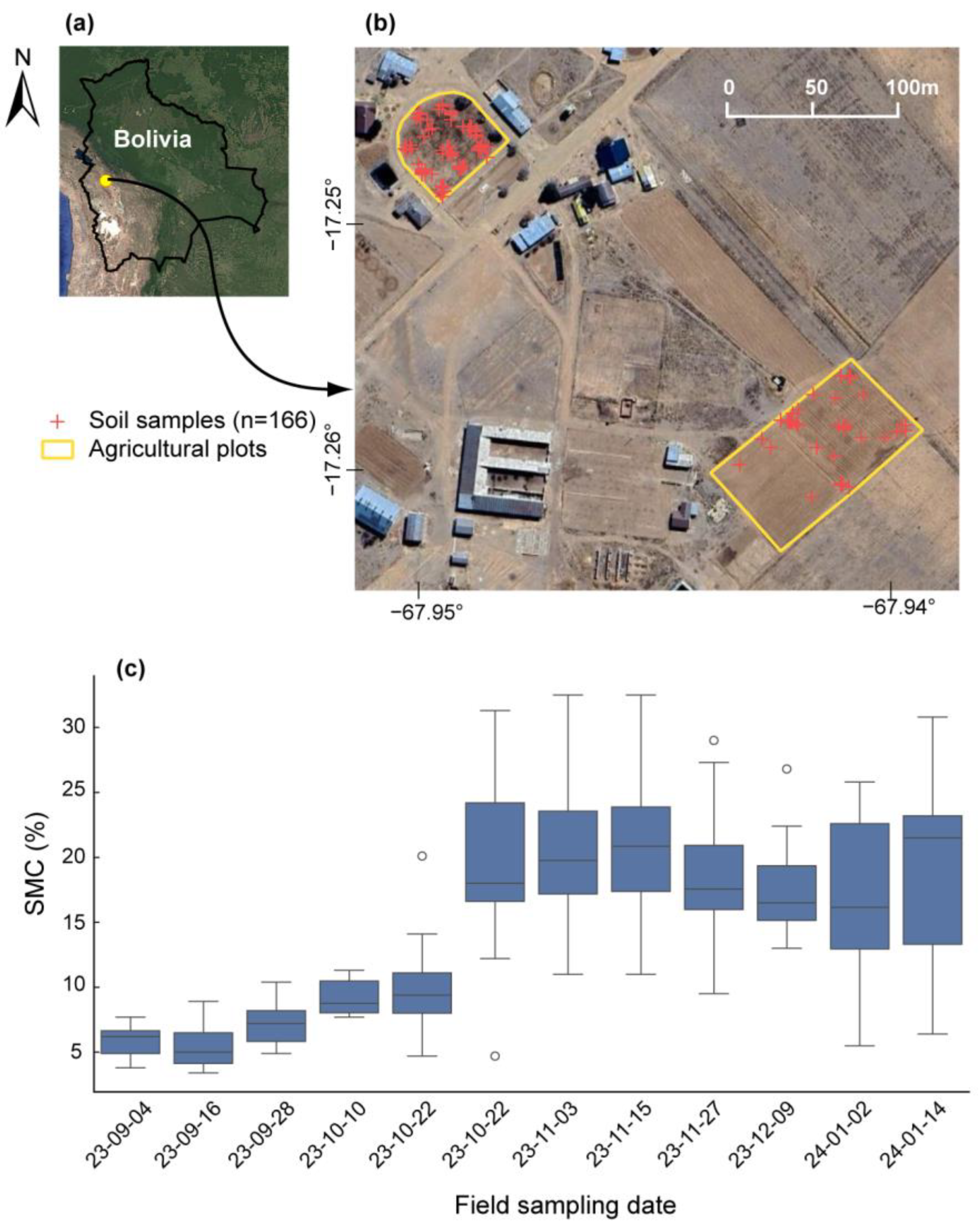
The research was conducted in two plots of approximately 6500 and 2540 m2 located at the Patacamaya experimental station from Universidad Mayor de San Andrés (UMSA) (Figure 1), located in the central Bolivian Altiplano region, at an average altitude of 3800 m.a.s.l. with a flat topography [39]. The region is semiarid with (i) an average rainfall of less than 400 mm∙year−1, concentrated in the austral summer [40], (ii) an average temperature that varies from 4 °C to 8 °C [41], and (iii) a high evapotranspiration rate of approximately 1300 mm∙year−1. Agriculture is the main economic activity, which increasingly depends on irrigation to cope with the water deficit [42]. According to World Reference Base for Soil (WRB) System guidelines, the soils are classified as Association of Leptosols—Durisols—Regosols [43].
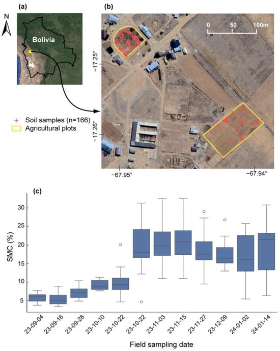
Figure 1.
The study area in Bolivia (a), along with the location of 166 soil sample sites within agricultural plots (b) and Boxplot of the volumetric soil moisture measurements obtained during the study period (c). White circle represent the outlier SMC measurements.
2.2. Reference Soil Moisture Data
A total of 166 soil samples were collected within the agricultural plots during twelve field visits starting on 4 September 2023 and ending on 14 January 2024. The visits (n = 12) were realized with a 12-day frequency to match with the S1 satellite observation dates and time (approximately 10 h local time) (Figure 1c). Twelve to fifteen soil samples were collected during each field visits. Each soil sample consists of a composite of 3 subsamples taken diagonally (upper left, center, lower right) from a 10 m × 10 m square area at 10 cm depth. Prior to soil sample collection, SMC was also measured using a TDR-150 Field Scout made by the Spectrum Technologies, Inc. (Aurora, CO, USA). Finally, two SMC measurement were obtained from each composite soil sample, one in the soil laboratory of the Faculty of Chemistry at Universidad Mayor de San Andrés (UMSA) by averaging the three soil samples’ information [10] and the other one from the TDR-150 Field Scout measurements.
2.3. Sentinel-1 Images and Pre-Processing
Sentinel-1 (S1) satellite images provide polarization values in VV (vertical/vertical) and VH (vertical/horizontal) in interferometry mode, with a center frequency of 5.405 GHz. S1 images are available as a Single Look Complex (SLC) product, which provides both phase and amplitude information, and as a post-processed Ground Range Detected (GRD) product, which provides direct surface backscatter in the form of intensity and amplitude images. Due to its dual-polarization antenna that can discriminate subtle changes in SMC, the GRD product has emerged as an essential tool for mapping soil moisture and is therefore being considered for the current study. S1 images are available from both ascending and descending orbits. To maintain consistency in S1 observations across space and time, only the descending orbit is used. All S1 images acquired during field soil sample collection were preprocessed according to four successive steps: (i) border noise removal, (ii) radiometric calibration, (iii) topographic correction, and (iv) focal mean filter to reduce the speckle effect. S1 preprocessing (i.e., downloading, preprocessing, and compositing) was carried out via GEE [44] on the free cloud platform Google Colab (retrieved from https://colab.research.google.com/, accessed on 20 October 2024). Finally, for each soil sampling date a composite image is obtained by averaging the value of two S1 images: the one acquired during the sampling date and the one obtained 12 days before.
2.4. Soil Moisture Active Passive (SMAP)
The SMAP mission is an orbiting satellite launched in January 2015 to measure soil moisture globally using an L-band radiometer. SMAP Level-4 (L4) soil moisture product provides global observations of SMC at different depths (e.g., 0–5 cm, 0–100 cm), along with other research outputs, such as soil temperature and evapotranspiration at high temporal resolution (every 3 h) and low spatial resolution (11 km) [45]. SMAP L4 ensures continuous data availability, even during instrument outages, by relying on land model simulations when necessary [46]. For this study we used SMAP L4 SMC of the top (0–5 cm) and root zone (0–100 cm) layers, both available on GEE.
2.5. Integrated Multi-Satellite Retrievals for GPM (IMERG)
The Global Precipitation Measurement (GPM) mission was launched in February 2014 as the successor to the Tropical Rainfall Measuring Mission (TRMM) [47]. Compared to the TRMM, the GPM enhances spatial resolution (from 0.25° to 0.1°) and temporal resolution (from 3 h to 30 min), expands coverage (from 50°N–50°S to 60°N–60°S), and improves sensitivity for detecting light and solid precipitation [48]. The Integrated Multi-satellitE Retrievals for GPM (IMERG) is the precipitation product derived from the GPM mission. IMERG reliability was previously assessed across the Altiplano region, and results show that IMERG precipitation estimates are reliable for daily total amount monitoring and hydrological modelling [41,49]. For this study, we used the last released version (v.07) available at the hourly time-step in GEE [50].
2.6. Machine Learning Models
Four supervised machine learning (ML) models based on decision trees were evaluated: (i) Random Forest (RF) [51], (ii) Extreme Gradient Boosting (XGB) [52], (iii) Decision Tree (DT) [53], and (iv) Gradient Boosting (GB) [54]. Decision trees are non-parametric supervised learning models commonly used for regression and classification tasks. These models represent decisions and their potential outcomes in a hierarchical structure analogous to a tree, allowing the derivation of simple decision rules from dataset features to predict a target variable (e.g., soil moisture) [55].
In the DT model, a single decision tree is built by recursively dividing the dataset into smaller subsets, using features that maximize information gain or reduce impurity [53,55]. The RF model employs an ensemble of decision trees, each trained on different subsets of the dataset using bagging (bootstrap aggregation). The final prediction is derived as the average of all tree predictions, enhancing model robustness and reducing overfitting [51]. The GB model builds decision trees sequentially, with each tree aiming to correct the errors of its predecessor by minimizing a defined loss function. This iterative process leverages the residuals of the prior tree to guide subsequent tree construction [54]. XGB is an advanced implementation of GB that incorporates parallel computing and regularization techniques, improving computational efficiency and mitigating overfitting [52].
All models were implemented using default hyper-parameters provided by a Python library [52,56], as these default configurations yielded satisfactory performance in the ML models [56]. Default hyper-parameter values are presented in Table 1.

Table 1.
Hyper-parameters considered for the machine learning models’ set-up.
3. Methods
3.1. Laboratory SMC Measurement
SMC was computed using both the gravimetric and volumetric methods. To do so, each soil sample was collected with a metal cylinder directly pushed all the way in from the surface before being removed. Then, the soil sample trapped in the metal cylinder was extracted into a polypropylene plastic container (150 mL), hermetically sealed, and directly brought to the laboratory for analysis. Each soil sample was (i) weighed to obtain humid mass (Mh), (ii) dried during 24 h at 105 °C, (iii) left to cool in a desiccant capsule to avoid absorption of moisture from the environment, and (iv) weighed again to obtain the dry mass (Md). Finally, gravimetric humidity was computed (Equation (1)) and converted to volumetric humidity (Equation (2)) to compare with TDR Field Scout SMC measurements. Hereafter, the volumetric humidity is considered as the reference SMC values.
where θg and θv represent the gravimetric and volumetric humidity, respectively, and ρa and ρw represents the bulk density of soil (1.48 g·cm−3 [57]) and the water density (1 g·cm−3), respectively.
3.2. TDR Measurement Assessment
SMC obtained through the TDR-150 Field Scout was compared to the SMC obtained in laboratory to assess TDR-150 Field Scout SMC reliability. The comparison is based on R2 and RMSE.
3.3. Learning Database Elaboration
Eight polarization indices (PIs) and 36 texture indices (TIs) were derived from all S1 single scenes and composite images (Table 2). Note that S1 TIs were derived from the Gray Level Co-occurrence Matrix (GLCM) available in GEE [58]. All these indices were selected because they have shown strong correlation with soil moisture [37,59,60,61]. SMAP top layer (0–5 cm) and root zone (0–100 cm) SMC obtained from the nearest time of the field measurement (13–14 h UTC-0), along with IMERG total precipitation amount for the 5-day period preceding the soil moisture measurements date, were considered.
Table 2.
Sentinel-1 features. Note that all indices were computed from both the S1 images acquired during field soil sampling (i.e., single scene) and the corresponding composite image.
Following this process, the learning database included 166 soil moisture observations with corresponding S1 features obtained from the single scenes (n = 46) and the composite images (n = 46), SMAP SMC (n = 2), and IMERG precipitation amount (n = 1) (Table 2 and Table 3).
Table 3.
Hydrological features.
3.4. Machine Learning Modelling Set-Up
First, SMAP and IMERG features (i.e., top layer SMC, root zone SMC, and total precipitation) were considered as independent features to assess their potential for SMC mapping across agriculture field (scenario-1). Then, S1 features were aggregated to the independent features to assess the potential improvement in SMC estimates brought by S1 features. To assess the potential of S1 features obtained from single scenes and composite images, different scenarios were considered. First, only S1 features obtained from the single scenes were considered (scenario-2); second, only S1 features obtained from the composite images were considered (scenario-3); and finally, S1 features obtained from both the single scenes and the composite images were considered (scenario-4) (Figure 2).
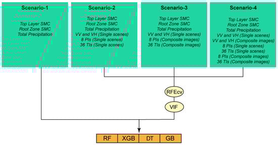
Figure 2.
SMC modeling framework flow chart. Note that the 8 PIs and 36 TIs were computed from both the S1 images acquire during field soil sampling and the corresponding composite image.
Multi-collinearity is a common issue in machine learning that reduces the robustness of models because of redundancy in the chosen independent features. To mitigate this, the Recursive Feature Elimination Cross Validation (RFEcv) algorithm was employed to identify the subset of independent features that provides the best performance [64]. As a model-specific feature selection technique (a wrapping method), RFEcv is executed independently for each model. The model undergoes iterative runs, eliminating one redundant feature at a time until the model’s performance experiences the smallest decline. In this process, the 10-fold cross-validation is used, with the Root Mean Square Error (RMSE, Equation (1)) serving as the objective function. Afterward, the Variance Inflation Factor (VIF) is applied to the subset of independent features selected by RFEcv to further reduce multi-collinearity. Only independent features with a VIF lower than 10 are retained [65]. This two-step feature selection process (RFEcv, VIF) was selected, as it considerably improved machine learning outputs [35]. It is worth mentioning that, due to the low number of independent features in scenario-1 (n = 3), no multi-collinearity issue was expected for this scenario, and therefore, the above-described two-step feature selection was only applied to scenario-2, -3, and -4.
Finally, each machine-learning model (RF, GT, GB, and XGB) was trained using 70% (n = 116) of the total learning database observations (n = 166) and validated using the remaining 30% of the observations (n = 50) not used during the training. The 70–30% splitting was based on a random selection among all available observations (n = 166). To ensure consistent comparisons among all the considered model and scenario combinations, the same splitting was used for all considered set-ups, so that each model and scenario combination was trained and validated with the exact same observations.
The models’ output reliability was assessed using the coefficient of determination (R2, Equation (3)) and the Root Mean Square Error (RMSE, Equation (4)).
where n represents the number of samples, and Pi and Oi represent the predicted and observed values of SMC at the site i, respectively, and represents the average of the observed values.
4. Results
4.1. TDR-150 Field Scout Reliability
Figure 3 shows the correlation between SMCs obtained (i) with the TDR-150 Field Scout and (ii) in laboratory (gravimetric method). With an R2 and an RMSE of 0.98 and 2.8%, respectively, the TDR-150 Field Scout provides reliable SMC estimates across the considered region. It is worth mentioning that laboratory SMC measurements are also subject to uncertainties because of the loss of humidity during the transport from the sampling site to the laboratory. In consequence, SMCs obtained through the TDR tend to be slightly superior to the SMCs obtained in the laboratory (Bias = 2.6%, Figure 3). According to this result, the SMCs obtained through the TDR-150 Field Scout are used as a reference (i.e., target) in this study.
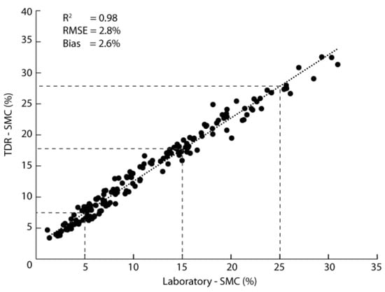
Figure 3.
Scatter plot of SMCs obtained in the laboratory and with TDR-150 Field Scout.
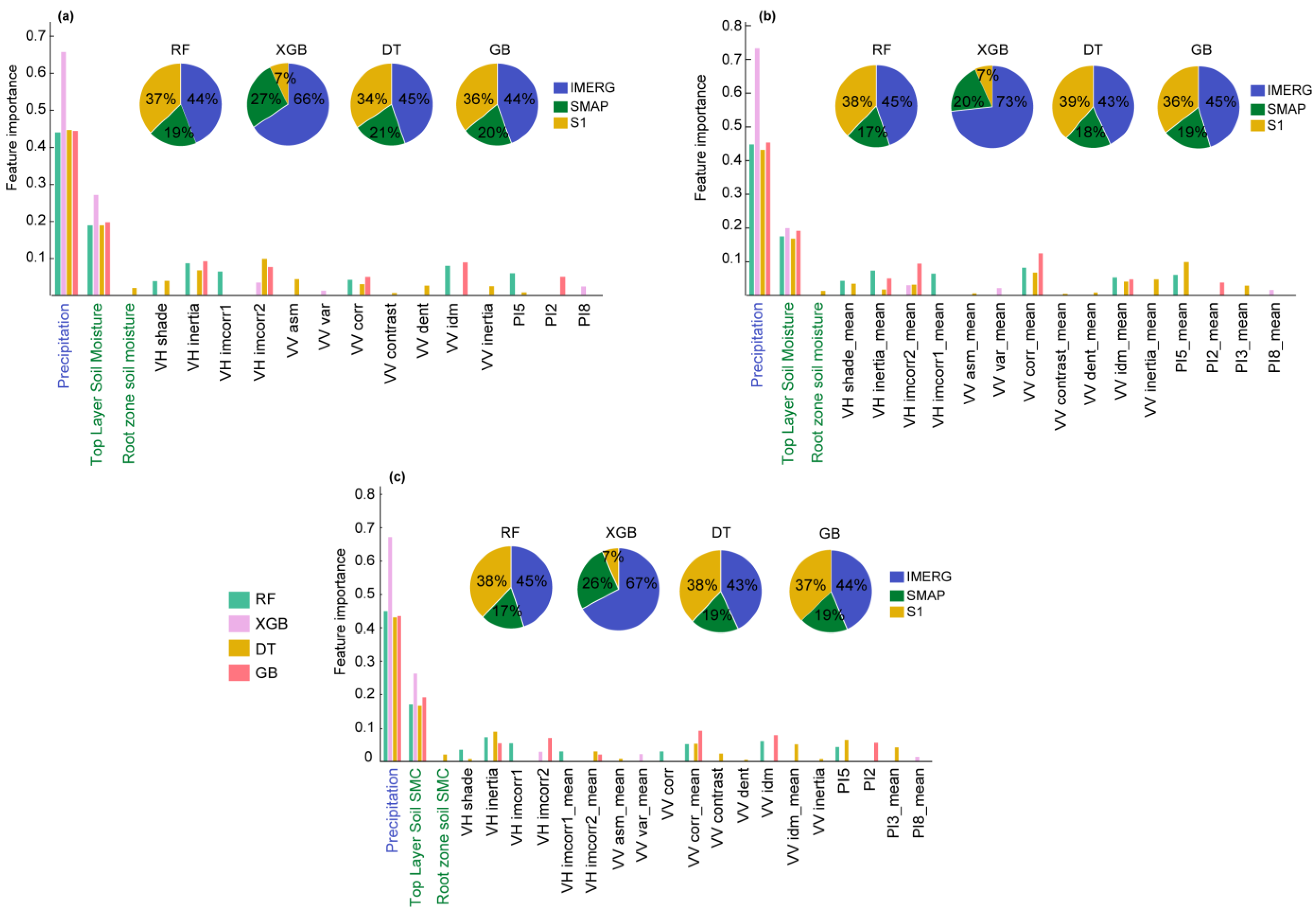
4.2. Feature Selection and Importance
Figure 4 shows the feature importance (FI) of the selected independent features for each model and scenario-2, -3, and -4 (SMAP + IMERG + S1). FI was obtained from the models during the training step. It quantifies the respective contribution of each independent variable in the output prediction. For all scenarios (-2, -3, and -4), “total precipitation” (IMERG) and “top layer soil moisture” (SMAP) were identified as the most relevant features, together accounting for more than 60% of the FI for all considered models and scenarios. Precipitation is of particular importance, because it is the main driver of SMC variations for the studied soils. Moreover, “root zone soil” SMC has a very low FI value (close to 0) for all scenarios and models, as (i) target observations are superficial, so not necessarily correlated to deeper SMC (i.e., “root zone soil” SMC), and (ii) “root zone soil” SMC, through the assimilation of SMAP observation, turns into a land surface model with its own uncertainties. It can be explained with the difference between “root zone soil” depth (0–100 cm) and SMC’s use as a target (0–10 cm). Actually, no clear relationship between top layer (0–10 cm) and in-depth layer (0–100 cm) SMC is observed across semi-arid regions, as the top layer SMC is expected to dry faster than the in-depth layer.
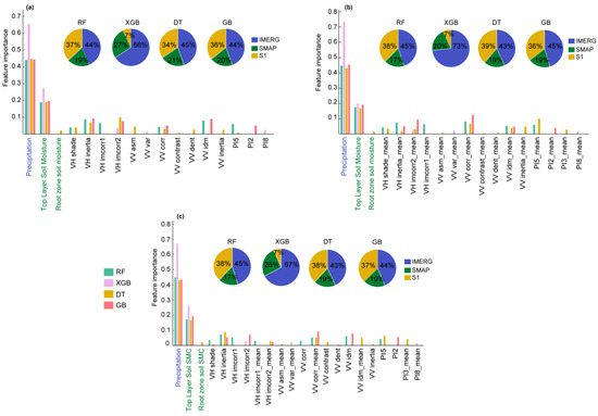
Figure 4.
Feature importance values for selected independent features and scenario-2, -3, and -4 (a,b,c, respectively), along with cumulative feature importance for IMERG, SMAP, and S1 independent features. Note that S1 features are computed with the composite images ending with “_mean”.
Even if S1 had been previously used to retrieve SMCs across different regions [9,36,37,38], only three (four) were selected for the modelling using scenario-2 (scenario-3 and -4). According to their equations (Table 2), all PIs are quite comparable, and therefore combining them is unlikely to offer any additional benefits.
Similarly, 11 (15) TIs were selected for the modelling using scenario-2 and -3 (scenario-4), with a majority of TIs based on VV. The dominance of VV TIs is in line with previous studies highlighting a higher SMC sensitivity to VV than to VH polarization [31,34,66]. It is worth mentioning that same TIs are selected for all scenarios, with some TIs (VH imcorr1, VH imcorr2, VV corr) considered twice in scenario-4 (i.e., derived from both the single scenes and composite images).
Finally, even if S1 independent features present low FI values (Figure 4), put together, they contribute approximately 7% to 39% in the modelling process (Figure 4). This indicates that S1 improves SMC estimates at higher spatial resolution (i.e., 20 m). Actually, IMERG and SMAP bring relevant information for the SMC temporal dynamic, whereas S1 brings relevant information for the SMC spatial dynamic.
4.3. Soil Moisture Estimates Evaluation
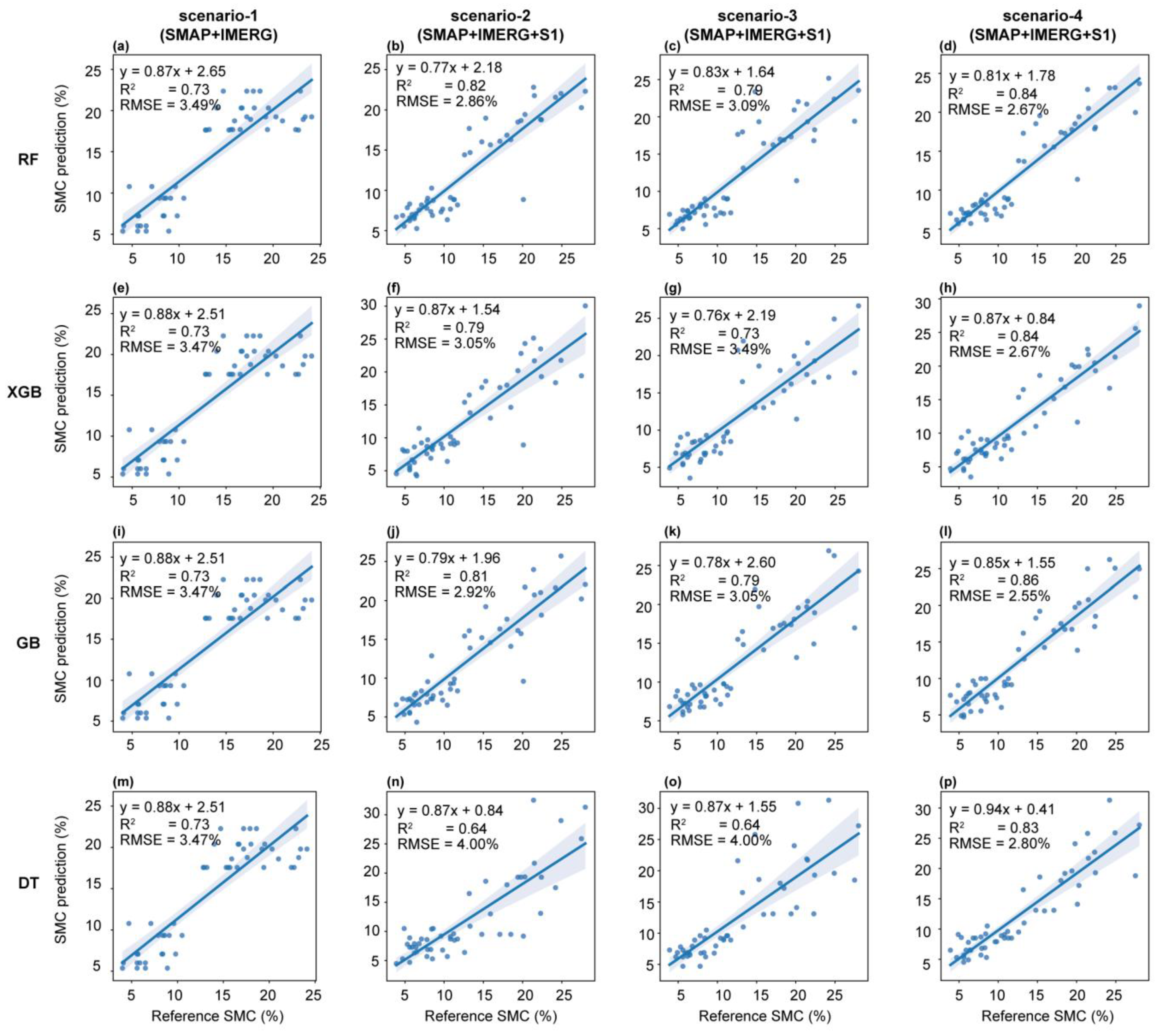
The comparison of scenario-1 with scenario-2, -3, and -4 shows that the integration of S1 features quite substantially improves the SMC estimates. Indeed, for each model, higher R2 and lower RMSE are obtained with scenario-2, -3, and -4.
Except for the DT model, the consideration of S1 features (scenario-2, -3, and -4) systematically improves the SMC estimates (Table 4). Even if composite images are generally recommended to minimize local noise [35,67,68], the results show that more reliable SMC estimates are obtained when considering the single scenes (scenario-2) rather than the composite images (scenario-3) (Table 4). Yet, the combination of the two (scenario-4) provides the most reliable SMC estimates for all considered models showing the complementarity of single scenes and composite images.
Table 4.
Performance of ML models with (SF) and without (TF) feature selection.
When comparing scenario-1 with scenario-4, an R2 increase of approximately 15%, 13.5%, 16%, and 12% is observed at the validation step for the RF, XGB, GB, and DT model, respectively. Similarly, an RMSE decrease of 15%, 14%, 18%, and 10% is observed at the validation step for the RF, XGB, GB, and DT model, respectively. These results underline the effectiveness of the S1 integration in the SMC mapping at high spatial resolution. Overall, based on scenario-4, all models provide reliable SMC estimates (R2 ≥ 0.83 and RMSE ≤ 3.15%), with GB performing the best (R2 = 0.86 and RMSE = 2.55%).
Scenario-1’s good fit (R2 ≥ 0.73) is due to an outlier compensation effect (Figure 5a,c,e,g) because the low spatial resolution of SMAP and IMERG (11 × 11 km) does not allow capturing SMC spatial variation occurring at the agriculture field level, as both considered plot fall in the same pixel. This is clearly observable through the horizontal line that corresponds to the same field sample collection date, for which SMAP and IMERG attribute the same value to all collected soil sample, whereas all these samples present very contrasted SMC values (Figure 5a,c,e,g). This aspect is considerably attenuated with the integration of S1 features (scenario-2, -3, and -4) (Figure 5). Actually, the high spatial resolution of S1 features (20 × 20 m) allows capturing SMC variation occurring for the same date at the agriculture field scale level and therefore the removal of the horizontal line (especially between 10% and 17.5% SMC, Figure 5b,d,f,h).
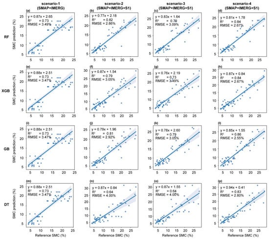
Figure 5.
Scatter plot comparing reference and prediction SMCs obtained with scenario-1, -2, -3, and -4 for the validation step with (a–d) RF, (e–h) XGB, (i–l) GB, and (m–p) DT.
This spatial discrepancy in between scenario-1 and scenario-2, -3, and -4 explains the overfitting issue observed in scenario-1 with lower (higher) R2 (RMSE) scores observed during the training step than during the validation step. Actually, the coarse spatial resolution of scenario-1 features (11 × 11 km) cannot capture the SMC spatial variability across the studied area. As a result, for each field visit, a unique combination of “root zone SMC”, “top layer SMC”, and “total precipitation” is attributed to all the SMCs observed that day at the different sampled points. As a result, when testing the models, the targeted SMC to predict has high probability to be included in the SMC range used in the training step, leading to an overfitting issue. This problem is avoided in scenario-2, -3, and -4 due to the consideration of the 20 m spatial resolution feature (S1), insuring a better discretization of the SMC spatial variability.
4.4. Soil Moisture Mapping
Figure 6 shows SMC maps derived from scenario-1 and -4 for 4 September 2023. It is worth mentioning that, as SMC maps derived from scenario-1 are similar for all considered models, Figure 6 only shows SMC maps obtained with the RF model. Similarly, as scenario-4 is more reliable than scenario-2 and -3 (Table 4, Figure 5), Figure 6 only shows maps obtained with scenario-4.
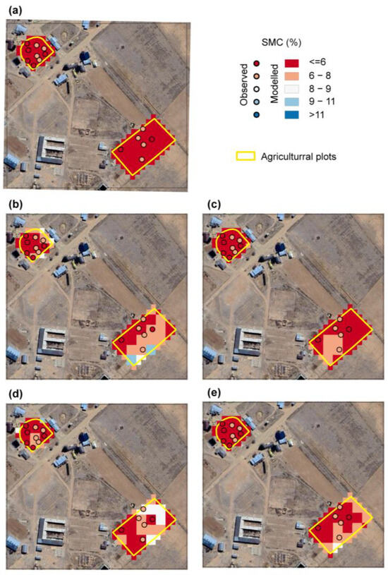
Figure 6.
4 September 2023 SMC maps derived from (a) RF with scenario-1, and using scenario-4 with (b) RF, (c) XGB, (d) GB, and (e) DT.
Due to SMAP’s and IMERG’s low spatial resolution (11 × 11 km), SMC maps based on scenario-1 show a uniformity in the study area (Figure 6a). Conversely, SMC maps based on scenario-4 present SMC variability in space that confirms the benefit of S1 features’ high spatial resolution (20 × 20 m) for the redistribution of SMAP SMC estimates (i.e., top layer soil moisture) at the sub-grid scale.
Although the models generated comparable metrics during the validation step (Table 4), significant differences are observed in the spatial distribution of the predicted SMCs. XGB and DT produced a more homogeneous SMC mapping in the agricultural plots, with values ranging between 6 and 8%. In contrast, RF shows a more marked variability in SMC, identifying sectors with up to 11% moisture. GB, on the other hand, reports a more balanced SMC distribution and greater agreement with reference SMC (Figure 6).
5. Discussion
Despite S1’s opportunity to substantially increase SMC estimates spatial resolution and accuracy (Figure 5 and Figure 6, Table 4), its 12-day revisit time does not allow daily monitoring. In this context, several studies combine daily MODIS optical/infrared and/or land surface temperature (LST) estimates to achieve continuous SMC estimates [18,25,26,27]. However, these MODIS datasets are available at coarse spatial resolution (i.e., 500 m) and for clear sky conditions. Therefore, high spatial (i.e., 20 m) and temporal (i.e., daily) resolution SMC mapping from satellite still represents a challenge to investigate.
Despite its low spatial resolution (11 km), IMERG precipitation estimates play a fundamental role in SMC mapping (Figure 3). Therefore, satellite-based precipitation estimates available at higher spatial resolution should considerably improve SMC mapping. As available satellite-based precipitation estimates across the region are only available at kilometric spatial resolution [69,70], a spatial downscaling procedure should be considered to obtaina precipitation estimates at high spatial resolution. In this line, the method proposed by [47] that integrates MODIS cloud optical and microphysical properties to improve IMERG spatial resolution from 11 km to 1 km could be used as a guideline. On the other hand, evapotranspiration (ET) is highly correlated with SMC in areas with poor vegetation cover [71]. Therefore, the integration of satellite-based ET estimates in the presented modelling approach should improve SMC estimates. Yet, satellite-based ET estimates rely on optical/IR data (i.e., SEBAL [72,73], SSEBop [74], METRIC [75]) that are only available for clear sky conditions, preventing daily monitoring.
Topography plays a crucial role in SMC dynamics [76], as it provides essential information for identifying depressions and areas prone to water accumulation, which in turn influence soil moisture levels. Numerous studies have demonstrated the benefits of incorporating topographic data as an independent variable in machine learning (ML) models for soil moisture mapping [77,78,79]. A study conducted in the UK found that using a high-resolution digital elevation model (DEM) derived from drone imagery significantly improved the reliability of ML models for predicting soil organic carbon in plowed fields [80]. Considering that microtopography in plowed areas is recognized as a key factor influencing the spatial distribution of soil moisture [81,82], incorporating such a detailed DEM could substantially enhance the performance and reliability of SMC predictions. It is worth mentioning here that freely available DEMs (i.e., SRTM) are not suitable for such a purpose. Indeed, these DEMs were retrieved from a single date, so the topography at that time might differ from the present one, especially across agriculture plots where plough practices considerably change microtopographic features.
In this study, the RFE wrapper features selection has been selected based on previous studies reporting on its efficiency [35,64]. However, other wrapper features selection such as the Genetic Algorithm (GA) or Sequential Feature Selector (SFS) have also proven their efficiency. Actually, the reliability of machine learning models (e.g., RF and Support Vector Machine (SVM)) significantly increases when using the GA or SFS with GA, being more suitable than SFS for SVM models [67,83]. Similarly, by default, hyper-parameter values have been used in this study for all the considered models (i.e., RF, XGB, GB, DT). However, hyper-parameters tuning techniques such as the grid-search function could be used to increase model performance and prevent model overfitting or underfitting [83,84,85,86,87]. In this context, future studies should consider combining hyper-parameter tuning with different feature-selection processes (i.e., RFE, GA, and SFS) to ensure an as efficient as possible modelling set-up.
Finally, this study relies on the consideration of single models. However, recently, machine learning model stacking strategies have been successfully applied to downscale SMAP SMC estimates to 1 km [38] and to estimated SMC at 30 m spatial resolution [88]. Both studies show that the stacking modelling approach outperforms the single modelling approach [38,88]. In this context, a stacking modelling approach integrating the above-mentioned datasets (i.e., high spatial resolution satellite-based precipitation, evapotranspiration, and digital elevation models) constitutes a very promising approach to substantially improve SMC mapping.
It is worth mentioning that S1 polarizations are not only sensitive to SMC but also to soil roughness and vegetation cover [89,90]. As the models were calibrated and validated across two agriculture plots with intrinsic soil roughness and vegetation cover, these models can only be used to estimate SMC across areas with similar features (i.e., soil roughness, vegetation cover). Indeed, different soil roughness and/or vegetation cover will result in different S1 polarization, even for a similar SMC range as the one considered in this study. As these models were not trained for such combinations, they will inevitably fail to retrieve SMC in different areas. To minimize such inconsistency, additional observations from areas with different soil roughness and vegetation cover should be added to the learning database.
6. Conclusions
This study assesses the integration of several remote sensing datasets (i.e., SMAP, IMERG and S1) in advanced machine learning techniques for Soil Moisture Content (SMC) mapping at high spatial resolution (20 m). For this task, different machine learning models (Random Forest—RF, Extreme Gradient Boosting—XGB, Gradient Boosting—GB, and Decision Tree—DT) are considered. The key findings can be summarized as follows:
- -
- Top-layer SMC derived from L-band sensors (i.e., SMAP) and precipitation (i.e., IMERG) are predominant factors in SMC monitoring.
- -
- Even if accurate SMC (R2 ≥ 0.73; RMSE ≤ 3.15%) can be obtained considering only precipitation and top-layer SMC, the coarse spatial resolution (i.e., 10 km) of these datasets cannot capture SMC spatial variation at the agriculture plot scale.
- -
- Adding S1-based features to IMERG precipitation and SMAP top-layer SMC substantially improved SMC estimates derived from all considered models, with an R2 (RMSE) increase (decrease) ranging from 12% to 16% (10% to 18%) depending on the considered model (with scenario-4).
- -
- S1-based features allow the spatial downscaling of SMC estimates obtained through SMAP and IMERG from 10 km to 20 m. In this process, S1 features derived from single scenes alone lead to more reliable SMC estimates than the consideration of S1 features derived from composite images alone, and the combination of the two provides the most reliable SMC estimates for all considered models.
- -
- Among the considered models, the GB model (with scenario-4) achieved the highest reliability, with an R2 and RMSE of 0.86 and 2.55%, respectively.
The significance of this research lies in its innovative application of remote sensing data and machine learning to address the challenges of SMC estimation at the agriculture plot level to provide a valuable tool for precision agriculture. By effectively downscaling SMAP data using Sentinel-1 (from 10 km to 20 m), our approach not only enhances spatial resolution but also improves the reliability of SMC estimates. The practical applications of these findings may support stakeholders and policymakers to make informed decisions about water resource management (i.e., irrigation) towards sustainable agriculture management strategies. The proposed framework can serve to assess the impacts of climate variability on SMC dynamics to provide complementary insights to support climate-resilient agricultural practices. Even if this study can serve as a blueprint for similar applications in different regions, further research should focus on refining this method by considering (i) the same independent features (i.e., precipitation, top layer SMC) at a higher spatial resolution, (ii) additional independent features, controlling SMC variability in space and time (e.g., evapotranspiration, soil properties), and (iii) more complex machine-learning approaches (e.g., stacking).
Author Contributions
Conceptualization, D.T., L.B. and F.S.; methodology, D.T., L.B. and F.S.; formal analysis, D.T. and L.B.; investigation, D.T., L.B., F.A., R.C., R.H., E.R., R.E.-V., R.P.Z., M.P.-F., E.U. and F.S.; data curation, D.T. and L.B.; writing—original draft preparation, D.T. and F.S.; writing—review and editing, D.T., L.B., F.A., R.C., R.H., E.R., R.E.-V., R.P.Z., M.P.-F., E.U. and F.S.; supervision F.S.; project administration, F.S.; funding acquisition, F.S. All authors have read and agreed to the published version of the manuscript.
Funding
This work was supported by the Agropolis Foundation (project number: 2001-032) in the framework of the project WASACA (Wastewater irrigation: a sustainable agriculture adaptation to climate changes over the Bolivian Altiplano?) and by the Centre National d’Etudes Spatiales (CNES) in the framework of the QUIMONOS project (Quinoa monitoring by satellite). The first author is grateful to the IRD (Institut de Recherche pour le Développement) for its financial support.
Data Availability Statement
The original contributions presented in the study are included in the article; further inquiries can be directed to the corresponding author.
Conflicts of Interest
The authors declare no conflicts of interest.
References
- Seneviratne, S.I.; Corti, T.; Davin, E.L.; Hirschi, M.; Jaeger, E.B.; Lehner, I.; Orlowsky, B.; Teuling, A.J. Investigating Soil Moisture–Climate Interactions in a Changing Climate: A Review. Earth-Sci. Rev. 2010, 99, 125–161. [Google Scholar] [CrossRef]
- Weil, R.; Brady, N. The Nature and Properties of Soils, 15th ed.; Pearson: New York, NY, USA, 2016; ISBN 978-0-13-325448-8. [Google Scholar]
- Bittelli, M. Measuring Soil Water Content: A Review. HortTechnology 2011, 21, 293–300. [Google Scholar] [CrossRef]
- Mueller, L.; Schindler, U.; Mirschel, W.; Shepherd, T.G.; Ball, B.C.; Helming, K.; Rogasik, J.; Eulenstein, F.; Wiggering, H. Assessing the Productivity Function of Soils. A Review. Agron. Sustain. Dev. 2010, 30, 601–614. [Google Scholar] [CrossRef]
- Cardoso, E.J.B.N.; Vasconcellos, R.L.F.; Bini, D.; Miyauchi, M.Y.H.; Santos, C.A.d.; Alves, P.R.L.; Paula, A.M.d.; Nakatani, A.S.; Pereira, J.d.M.; Nogueira, M.A. Soil Health: Looking for Suitable Indicators. What Should Be Considered to Assess the Effects of Use and Management on Soil Health? Sci. Agric. 2013, 70, 274–289. [Google Scholar] [CrossRef]
- Carrão, H.; Russo, S.; Sepulcre-Canto, G.; Barbosa, P. An Empirical Standardized Soil Moisture Index for Agricultural Drought Assessment from Remotely Sensed Data. Int. J. Appl. Earth Obs. Geoinf. 2016, 48, 74–84. [Google Scholar] [CrossRef]
- Shaxson, F.; Barber, R. Optimizing Soil Moisture for Plant Production: The Significance of Soil Porosity; FAO Soil Bulletin; Food and Agriculture Organization of the United Nations (FAO): Rome, Italy, 2003; ISBN 92-5-104944-0. [Google Scholar]
- Rasheed, M.W.; Tang, J.; Sarwar, A.; Shah, S.; Saddique, N.; Khan, M.U.; Imran Khan, M.; Nawaz, S.; Shamshiri, R.R.; Aziz, M.; et al. Soil Moisture Measuring Techniques and Factors Affecting the Moisture Dynamics: A Comprehensive Review. Sustainability 2022, 14, 11538. [Google Scholar] [CrossRef]
- Senanayake, I.P.; Pathira Arachchilage, K.R.L.; Yeo, I.-Y.; Khaki, M.; Han, S.-C.; Dahlhaus, P.G. Spatial Downscaling of Satellite-Based Soil Moisture Products Using Machine Learning Techniques: A Review. Remote Sens. 2024, 16, 2067. [Google Scholar] [CrossRef]
- FAO. Standard Operating Procedure for Soil Organic Moisture Content by Gravimetric Method, 1st ed.; Global Soil Laboratory Network GLOSOLAN; FAO: Rome, Italy, 2023. [Google Scholar]
- Mohanty, B.P.; Skaggs, T.H. Spatio-Temporal Evolution and Time-Stable Characteristics of Soil Moisture within Remote Sensing Footprints with Varying Soil, Slope, and Vegetation. Adv. Water Resour. 2001, 24, 1051–1067. [Google Scholar] [CrossRef]
- Brocca, L.; Morbidelli, R.; Melone, F.; Moramarco, T. Soil Moisture Spatial Variability in Experimental Areas of Central Italy. J. Hydrol. 2007, 333, 356–373. [Google Scholar] [CrossRef]
- Crow, W.T.; Berg, A.A.; Cosh, M.H.; Loew, A.; Mohanty, B.P.; Panciera, R.; de Rosnay, P.; Ryu, D.; Walker, J.P. Upscaling Sparse Ground-Based Soil Moisture Observations for the Validation of Coarse-Resolution Satellite Soil Moisture Products. Rev. Geophys. 2012, 50, RG2002. [Google Scholar] [CrossRef]
- He, H.; Aogu, K.; Li, M.; Xu, J.; Sheng, W.; Jones, S.B.; González-Teruel, J.D.; Robinson, D.A.; Horton, R.; Bristow, K.; et al. Chapter Three—A Review of Time Domain Reflectometry (TDR) Applications in Porous Media. In Advances in Agronomy; Sparks, D.L., Ed.; Academic Press: Cambridge, MA, USA, 2021; Volume 168, pp. 83–155. [Google Scholar]
- Patterson, D.E.; Smith, M.W. Unfrozen Water Content in Saline Soils: Results Using Time-Domain Reflectometry. Can. Geotech. J. 1985, 22, 95–101. [Google Scholar] [CrossRef]
- Zegelin, S.J.; White, I.; Jenkins, D.R. Improved Field Probes for Soil Water Content and Electrical Conductivity Measurement Using Time Domain Reflectometry. Water Resour. Res. 1989, 25, 2367–2376. [Google Scholar] [CrossRef]
- Wang, L.; Qu, J.J. Satellite Remote Sensing Applications for Surface Soil Moisture Monitoring: A Review. Front. Earth Sci. China 2009, 3, 237–247. [Google Scholar] [CrossRef]
- Millard, K.; Richardson, M. Quantifying the Relative Contributions of Vegetation and Soil Moisture Conditions to Polarimetric C-Band SAR Response in a Temperate Peatland. Remote Sens. Environ. 2018, 206, 123–138. [Google Scholar] [CrossRef]
- Njoku, E.G.; Kong, J.-A. Theory for Passive Microwave Remote Sensing of Near-Surface Soil Moisture. J. Geophys. Res. 1896–1977 1977, 82, 3108–3118. [Google Scholar] [CrossRef]
- Portal, G.; Jagdhuber, T.; Vall-llossera, M.; Camps, A.; Pablos, M.; Entekhabi, D.; Piles, M. Assessment of Multi-Scale SMOS and SMAP Soil Moisture Products across the Iberian Peninsula. Remote Sens. 2020, 12, 570. [Google Scholar] [CrossRef]
- Akash, M.; Mohan Kumar, P.; Bhaskar, P.; Deepthi, P.R.; Sukhdev, A. Review of Estimation of Soil Moisture Using Active Microwave Remote Sensing Technique. Remote Sens. Appl. Soc. Environ. 2024, 33, 101118. [Google Scholar] [CrossRef]
- Rowlandson, T.; Impera, S.; Belanger, J.; Berg, A.A.; Toth, B.; Magagi, R. Use of in Situ Soil Moisture Network for Estimating Regional-Scale Soil Moisture during High Soil Moisture Conditions. Can. Water Resour. J. Rev. Can. Ressour. Hydr. 2015, 40, 343–351. [Google Scholar] [CrossRef]
- Wang, X.; Lü, H.; Crow, W.T.; Zhu, Y.; Wang, Q.; Su, J.; Zheng, J.; Gou, Q. Assessment of SMOS and SMAP Soil Moisture Products against New Estimates Combining Physical Model, a Statistical Model, and in-Situ Observations: A Case Study over the Huai River Basin, China. J. Hydrol. 2021, 598, 126468. [Google Scholar] [CrossRef]
- Fang, B.; Lakshmi, V.; Zhang, R. Validation of Downscaled 1-Km SMOS and SMAP Soil Moisture Data in 2010–2021. Vadose Zone J. 2024, 23, e20305. [Google Scholar] [CrossRef]
- Carlson, T. An Overview of the “Triangle Method” for Estimating Surface Evapotranspiration and Soil Moisture from Satellite Imagery. Sensors 2007, 7, 1612–1629. [Google Scholar] [CrossRef]
- Zhan, Z.; Qin, Q.; Ghulan, A.; Wang, D. NIR-Red Spectral Space Based New Method for Soil Moisture Monitoring. Sci. China Ser. Earth Sci. 2007, 50, 283–289. [Google Scholar] [CrossRef]
- Sadeghi, M.; Babaeian, E.; Tuller, M.; Jones, S.B. The Optical Trapezoid Model: A Novel Approach to Remote Sensing of Soil Moisture Applied to Sentinel-2 and Landsat-8 Observations. Remote Sens. Environ. 2017, 198, 52–68. [Google Scholar] [CrossRef]
- Baghdadi, N.; El Hajj, M.; Zribi, M.; Bousbih, S. Calibration of the Water Cloud Model at C-Band for Winter Crop Fields and Grasslands. Remote Sens. 2017, 9, 969. [Google Scholar] [CrossRef]
- Hornacek, M.; Wagner, W.; Sabel, D.; Truong, H.-L.; Snoeij, P.; Hahmann, T.; Diedrich, E.; Doubkova, M. Potential for High Resolution Systematic Global Surface Soil Moisture Retrieval via Change Detection Using Sentinel-1. IEEE J. Sel. Top. Appl. Earth Obs. Remote Sens. 2012, 5, 1303–1311. [Google Scholar] [CrossRef]
- Gao, Q.; Zribi, M.; Escorihuela, M.J.; Baghdadi, N. Synergetic Use of Sentinel-1 and Sentinel-2 Data for Soil Moisture Mapping at 100 m Resolution. Sensors 2017, 17, 1966. [Google Scholar] [CrossRef] [PubMed]
- El Hajj, M.; Baghdadi, N.; Zribi, M.; Bazzi, H. Synergic Use of Sentinel-1 and Sentinel-2 Images for Operational Soil Moisture Mapping at High Spatial Resolution over Agricultural Areas. Remote Sens. 2017, 9, 1292. [Google Scholar] [CrossRef]
- Wang, J.; Wu, F.; Shang, J.; Zhou, Q.; Ahmad, I.; Zhou, G. Saline Soil Moisture Mapping Using Sentinel-1A Synthetic Aperture Radar Data and Machine Learning Algorithms in Humid Region of China’s East Coast. CATENA 2022, 213, 106189. [Google Scholar] [CrossRef]
- Chung, J.; Lee, Y.; Kim, J.; Jung, C.; Kim, S. Soil Moisture Content Estimation Based on Sentinel-1 SAR Imagery Using an Artificial Neural Network and Hydrological Components. Remote Sens. 2022, 14, 465. [Google Scholar] [CrossRef]
- Baghdadi, N.; El Hajj, M.; Choker, M.; Zribi, M.; Bazzi, H.; Vaudour, E.; Gilliot, J.-M.; Ebengo, D.M. Potential of Sentinel-1 Images for Estimating the Soil Roughness over Bare Agricultural Soils. Water 2018, 10, 131. [Google Scholar] [CrossRef]
- Tola, D.; Satgé, F.; Pillco Zolá, R.; Sainz, H.; Condori, B.; Miranda, R.; Yujra, E.; Molina-Carpio, J.; Hostache, R.; Espinoza-Villar, R. Soil Salinity Mapping of Plowed Agriculture Lands Combining Radar Sentinel-1 and Optical Sentinel-2 with Topographic Data in Machine Learning Models. Remote Sens. 2024, 16, 3456. [Google Scholar] [CrossRef]
- Bai, J.; Cui, Q.; Zhang, W.; Meng, L. An Approach for Downscaling SMAP Soil Moisture by Combining Sentinel-1 SAR and MODIS Data. Remote Sens. 2019, 11, 2736. [Google Scholar] [CrossRef]
- Meyer, R.; Zhang, W.; Kragh, S.J.; Andreasen, M.; Jensen, K.H.; Fensholt, R.; Stisen, S.; Looms, M.C. Exploring the Combined Use of SMAP and Sentinel-1 Data for Downscaling Soil Moisture beyond the 1 Km Scale. Hydrol. Earth Syst. Sci. 2022, 26, 3337–3357. [Google Scholar] [CrossRef]
- Xu, J.; Su, Q.; Li, X.; Ma, J.; Song, W.; Zhang, L.; Su, X. A Spatial Downscaling Framework for SMAP Soil Moisture Based on Stacking Strategy. Remote Sens. 2024, 16, 200. [Google Scholar] [CrossRef]
- Satge, F.; Denezine, M.; Pillco, R.; Timouk, F.; Pinel, S.; Molina, J.; Garnier, J.; Seyler, F.; Bonnet, M.-P. Absolute and Relative Height-Pixel Accuracy of SRTM-GL1 over the South American Andean Plateau. ISPRS J. Photogramm. Remote Sens. 2016, 121, 157–166. [Google Scholar] [CrossRef]
- Garcia, M.; Raes, D.; Jacobsen, S.-E. Evapotranspiration Analysis and Irrigation Requirements of Quinoa (Chenopodium quinoa) in the Bolivian Highlands. Agric. Water Manag. 2003, 60, 119–134. [Google Scholar] [CrossRef]
- Satgé, F.; Pillco, R.; Molina-Carpio, J.; Mollinedo, P.P.; Bonnet, M.-P. Reliability of Gridded Temperature Datasets to Monitor Surface Air Temperature Variability over Bolivia. Int. J. Climatol. 2023, 43, 6191–6206. [Google Scholar] [CrossRef]
- Canedo, C.; Pillco Zolá, R.; Berndtsson, R. Role of Hydrological Studies for the Development of the TDPS System. Water 2016, 8, 144. [Google Scholar] [CrossRef]
- IUSS. World Reference Base for Soil Resources. International Soil Classification System for Naming Soils and Creating Legends for Soil Maps, 4th ed.; International Union of Soil Sciences (IUSS): Viena, Austria, 2022; ISBN 979-8-9862451-1-9. [Google Scholar]
- Gorelick, N.; Hancher, M.; Dixon, M.; Ilyushchenko, S.; Thau, D.; Moore, R. Google Earth Engine: Planetary-Scale Geospatial Analysis for Everyone. Remote Sens. Environ. 2017, 202, 18–27. [Google Scholar] [CrossRef]
- Reichle, R.; De Lannoy, G.; Koster, R.; Crow, W.; Kimball, J.; Liu, Q.; Bechtold, M. SMAP L4 Global 3-Hourly 9 Km EASE-Grid Surface and Root Zone Soil Moisture Geophysical Data, Version 7. 2022. Available online: https://nsidc.org/data/spl4smau/versions/7 (accessed on 15 February 2024).
- Entekhabi, D.; Njoku, E.G.; O’Neill, P.E.; Kellogg, K.H.; Crow, W.T.; Edelstein, W.N.; Entin, J.K.; Goodman, S.D.; Jackson, T.J.; Johnson, J.; et al. The Soil Moisture Active Passive (SMAP) Mission. Proc. IEEE 2010, 98, 704–716. [Google Scholar] [CrossRef]
- Callaú Medrano, S.; Satgé, F.; Molina-Carpio, J.; Pillco Zolá, R.; Bonnet, M.-P. Downscaling Daily Satellite-Based Precipitation Estimates Using MODIS Cloud Optical and Microphysical Properties in Machine-Learning Models. Atmosphere 2023, 14, 1349. [Google Scholar] [CrossRef]
- Huffman, G.J.; Bolvin, D.T.; Braithwaite, D.; Hsu, K.-L.; Joyce, R.J.; Kidd, C.; Nelkin, E.J.; Sorooshian, S.; Stocker, E.F.; Tan, J.; et al. Integrated Multi-Satellite Retrievals for the Global Precipitation Measurement (GPM) Mission (IMERG). In Satellite Precipitation Measurement: Volume 1; Levizzani, V., Kidd, C., Kirschbaum, D.B., Kummerow, C.D., Nakamura, K., Turk, F.J., Eds.; Springer International Publishing: Cham, Switzerland, 2020; pp. 343–353. ISBN 978-3-030-24568-9. [Google Scholar]
- Satgé, F.; Xavier, A.; Pillco Zolá, R.; Hussain, Y.; Timouk, F.; Garnier, J.; Bonnet, M.-P. Comparative Assessments of the Latest GPM Mission’s Spatially Enhanced Satellite Rainfall Products over the Main Bolivian Watersheds. Remote Sens. 2017, 9, 369. [Google Scholar] [CrossRef]
- Huffman, G.J.; Stocker, E.F.; Bolvin, D.T.; Nelkin, E.J.; Tan, J. GES DISC Dataset: GPM IMERG Final Precipitation L3 Half Hourly 0.1 Degree x 0.1 Degree V07 (GPM_3IMERGHH 07). 2023. Available online: https://rda.ucar.edu/datasets/d731000/ (accessed on 12 March 2024).
- Breiman, L. Random Forests. Mach. Learn. 2001, 45, 5–32. [Google Scholar] [CrossRef]
- Chen, T.; Guestrin, C. XGBoost: A Scalable Tree Boosting System. In Proceedings of the 22nd ACM SIGKDD International Conference on Knowledge Discovery and Data Mining, San Francisco, CA, USA, 13–17 August 2016; pp. 785–794. [Google Scholar]
- Quinlan, J.R. Induction of Decision Trees. Mach. Learn. 1986, 1, 81–106. [Google Scholar] [CrossRef]
- Friedman, J.H. Greedy Function Approximation: A Gradient Boosting Machine. Ann. Stat. 2001, 29, 1189–1232. [Google Scholar] [CrossRef]
- Breiman, L.; Friedman, J.; Olshen, R.A.; Stone, C.J. Classification and Regression Trees; Chapman and Hall/CRC: New York, NY, USA, 2017; ISBN 978-1-315-13947-0. [Google Scholar]
- Pedregosa, F.; Varoquaux, G.; Gramfort, A.; Michel, V.; Thirion, B.; Grisel, O.; Blondel, M.; Prettenhofer, P.; Weiss, R.; Dubourg, V.; et al. Scikit-Learn: Machine Learning in Python. J. Mach. Learn. Res. 2011, 12, 2825–2830. [Google Scholar]
- Vargas, E.R.; Céspedes, R. Clasificación de suelos según la aptitud de riego en la estación experimental Patacamaya. Rev. Investig. Innov. Agropecu. Recur. Nat. 2019, 6, 72–80. [Google Scholar]
- Haralick, R.M.; Shanmugam, K.; Dinstein, I. Textural Features for Image Classification. IEEE Trans. Syst. Man Cybern. 1973, SMC-3, 610–621. [Google Scholar] [CrossRef]
- Attarzadeh, R.; Amini, J.; Notarnicola, C.; Greifeneder, F. Synergetic Use of Sentinel-1 and Sentinel-2 Data for Soil Moisture Mapping at Plot Scale. Remote Sens. 2018, 10, 1285. [Google Scholar] [CrossRef]
- Mohseni, F.; Mirmazloumi, S.M.; Mokhtarzade, M.; Jamali, S.; Homayouni, S. Global Evaluation of SMAP/Sentinel-1 Soil Moisture Products. Remote Sens. 2022, 14, 4624. [Google Scholar] [CrossRef]
- Reichle, R.H.; Liu, Q.; Ardizzone, J.V.; Crow, W.T.; Lannoy, G.J.M.D.; Kimball, J.S.; Koster, R.D. IMERG Precipitation Improves the SMAP Level-4 Soil Moisture Product. J. Hydrometeorol. 2023, 24, 1699–1723. [Google Scholar] [CrossRef]
- Periasamy, S.; Ravi, K.P.; Tansey, K. Identification of Saline Landscapes from an Integrated SVM Approach from a Novel 3-D Classification Schema Using Sentinel-1 Dual-Polarized SAR Data. Remote Sens. Environ. 2022, 279, 113144. [Google Scholar] [CrossRef]
- Conners, R.W.; Trivedi, M.M.; Harlow, C.A. Segmentation of a High-Resolution Urban Scene Using Texture Operators. Comput. Vis. Graph. Image Process. 1984, 25, 273–310. [Google Scholar] [CrossRef]
- Awad, M.; Fraihat, S. Recursive Feature Elimination with Cross-Validation with Decision Tree: Feature Selection Method for Machine Learning-Based Intrusion Detection Systems. J. Sens. Actuator Netw. 2023, 12, 67. [Google Scholar] [CrossRef]
- Murray, L.; Nguyen, H.; Lee, Y.-F.; Remmenga, M.; Smith, D. Variance Inflation Factors in Regression Models with Dummy Variables. In Proceedings of the 2012—24th Annual Conference Proceedings, Conference on Applied Statistics in Agriculture, Foz do Iguacu, Brazil, 18–24 August 2012; pp. 161–177. [Google Scholar] [CrossRef]
- Bousbih, S.; Zribi, M.; El Hajj, M.; Baghdadi, N.; Lili-Chabaane, Z.; Gao, Q.; Fanise, P. Soil Moisture and Irrigation Mapping in A Semi-Arid Region, Based on the Synergetic Use of Sentinel-1 and Sentinel-2 Data. Remote Sens. 2018, 10, 1953. [Google Scholar] [CrossRef]
- Sirpa-Poma, J.W.; Satgé, F.; Resongles, E.; Pillco-Zolá, R.; Molina-Carpio, J.; Flores Colque, M.G.; Ormachea, M.; Pacheco Mollinedo, P.; Bonnet, M.-P. Towards the Improvement of Soil Salinity Mapping in a Data-Scarce Context Using Sentinel-2 Images in Machine-Learning Models. Sensors 2023, 23, 9328. [Google Scholar] [CrossRef] [PubMed]
- Sirpa-Poma, J.W.; Satgé, F.; Pillco, R.; Resongles, E.; Perez-Flores, M.; Flores, M.G.; Molina-Carpio, J.; Ramos, O.; Bonnet, M.-P. Complementarity of Sentinel-1 and Sentinel-2 Data for Soil Sa-Linity Monitoring to Support Sustainable Agriculture Practices in the Central Bolivian Altiplano (in Review). Sustainability 2024, 16, 6200. [Google Scholar] [CrossRef]
- Satgé, F.; Ruelland, D.; Bonnet, M.-P.; Molina, J.; Pillco, R. Consistency of Satellite-Based Precipitation Products in Space and over Time Compared with Gauge Observations and Snow-Hydrological Modelling in the Lake Titicaca Region. Hydrol. Earth Syst. Sci. 2019, 23, 595–619. [Google Scholar] [CrossRef]
- Satgé, F.; Hussain, Y.; Molina-Carpio, J.; Pillco, R.; Laugner, C.; Akhter, G.; Bonnet, M.-P. Reliability of SM2RAIN Precipitation Datasets in Comparison to Gauge Observations and Hydrological Modelling over Arid Regions. Int. J. Climatol. 2021, 41, E517–E536. [Google Scholar] [CrossRef]
- Bing, L.; Su, H.; Shao, Q.; Liu, J. Changing Characteristic of Land Surface Evapotranspiration and Soil Moisture in China during the Past 30 Years. J. Geo-Inf. Sci. 2012, 14, 1–13. [Google Scholar] [CrossRef]
- Bastiaanssen, W.G.M.; Molden, D.J.; Makin, I.W. Remote Sensing for Irrigated Agriculture: Examples from Research and Possible Applications. Agric. Water Manag. 2000, 46, 137–155. [Google Scholar] [CrossRef]
- Laipelt, L.; Henrique Bloedow Kayser, R.; Santos Fleischmann, A.; Ruhoff, A.; Bastiaanssen, W.; Erickson, T.A.; Melton, F. Long-Term Monitoring of Evapotranspiration Using the SEBAL Algorithm and Google Earth Engine Cloud Computing. ISPRS J. Photogramm. Remote Sens. 2021, 178, 81–96. [Google Scholar] [CrossRef]
- Senay, G. Satellite Psychrometric Formulation of the Operational Simplified Surface Energy Balance (SSEBop) Model for Quantifying and Mapping Evapotranspiration. Appl. Eng. Agric. 2018, 3, 555–566. [Google Scholar] [CrossRef]
- Allen, R.G.; Tasumi, M.; Trezza, R. Satellite-Based Energy Balance for Mapping Evapotranspiration with Internalized Calibration (METRIC)—Model. J. Irrig. Drain. Eng. 2007, 133, 380–394. [Google Scholar] [CrossRef]
- Raduła, M.W.; Szymura, T.H.; Szymura, M. Topographic Wetness Index Explains Soil Moisture Better than Bioindication with Ellenberg’s Indicator Values. Ecol. Indic. 2018, 85, 172–179. [Google Scholar] [CrossRef]
- Guevara, M.; Vargas, R. Downscaling Satellite Soil Moisture Using Geomorphometry and Machine Learning. PLoS ONE 2019, 14, e0219639. [Google Scholar] [CrossRef]
- Celik, M.F.; Isik, M.S.; Yuzugullu, O.; Fajraoui, N.; Erten, E. Soil Moisture Prediction from Remote Sensing Images Coupled with Climate, Soil Texture and Topography via Deep Learning. Remote Sens. 2022, 14, 5584. [Google Scholar] [CrossRef]
- Singh, A.; Gaurav, K. Deep Learning and Data Fusion to Estimate Surface Soil Moisture from Multi-Sensor Satellite Images. Sci. Rep. 2023, 13, 2251. [Google Scholar] [CrossRef]
- Cutting, B.J.; Atzberger, C.; Gholizadeh, A.; Robinson, D.A.; Mendoza-Ulloa, J.; Marti-Cardona, B. Remote Quantification of Soil Organic Carbon: Role of Topography in the Intra-Field Distribution. Remote Sens. 2024, 16, 1510. [Google Scholar] [CrossRef]
- Kamphorst, E.C.; Jetten, V.; Guérif, J.; Pitkänen, J.; Iversen, B.V.; Douglas, J.T.; Paz, A. Predicting Depressional Storage from Soil Surface Roughness. Soil Sci. Soc. Am. J. 2000, 64, 1749–1758. [Google Scholar] [CrossRef]
- Zhang, D.; Zhao, Y.; Qi, H.; Shan, L.; Chen, G.; Ning, T. Effects of Micro-Topography and Vegetation on Soil Moisture on Fixed Sand Dunes in Tengger Desert, China. Plants 2024, 13, 1571. [Google Scholar] [CrossRef]
- Taghadosi, M.M.; Hasanlou, M.; Eftekhari, K. Retrieval of Soil Salinity from Sentinel-2 Multispectral Imagery. Eur. J. Remote Sens. 2019, 52, 138–154. [Google Scholar] [CrossRef]
- Huang, Z.; Wu, W.; Liu, H.; Zhang, W.; Hu, J. Identifying Dynamic Changes in Water Surface Using Sentinel-1 Data Based on Genetic Algorithm and Machine Learning Techniques. Remote Sens. 2021, 13, 3745. [Google Scholar] [CrossRef]
- Bandak, S.; Movahedi Naeini, S.A.R.; Komaki, C.B.; Verrelst, J.; Kakooei, M.; Mahmoodi, M.A. Satellite-Based Estimation of Soil Moisture Content in Croplands: A Case Study in Golestan Province, North of Iran. Remote Sens. 2023, 15, 2155. [Google Scholar] [CrossRef]
- Zhang, W.; Liu, H.; Wu, W.; Zhan, L.; Wei, J. Mapping Rice Paddy Based on Machine Learning with Sentinel-2 Multi-Temporal Data: Model Comparison and Transferability. Remote Sens. 2020, 12, 1620. [Google Scholar] [CrossRef]
- Pham, L.H.; Pham, L.T.; Dang, T.D.; Tran, D.D.; Dinh, T.Q. Application of Sentinel-1 Data in Mapping Land-Use and Land Cover in a Complex Seasonal Landscape: A Case Study in Coastal Area of Vietnamese Mekong Delta. Geocarto Int. 2022, 37, 3743–3760. [Google Scholar] [CrossRef]
- Das, B.; Rathore, P.; Roy, D.; Chakraborty, D.; Jatav, R.S.; Sethi, D.; Kumar, P. Comparison of Bagging, Boosting and Stacking Algorithms for Surface Soil Moisture Mapping Using Optical-Thermal-Microwave Remote Sensing Synergies. CATENA 2022, 217, 106485. [Google Scholar] [CrossRef]
- Zheng, X.; Feng, Z.; Li, L.; Li, B.; Jiang, T.; Li, X.; Li, X.; Chen, S. Simultaneously Estimating Surface Soil Moisture and Roughness of Bare Soils by Combining Optical and Radar Data. Int. J. Appl. Earth Obs. Geoinf. 2021, 100, 102345. [Google Scholar] [CrossRef]
- Gella, G.W.; Bijker, W.; Belgiu, M. Mapping Crop Types in Complex Farming Areas Using SAR Imagery with Dynamic Time Warping. ISPRS J. Photogramm. Remote Sens. 2021, 175, 171–183. [Google Scholar] [CrossRef]


Disclaimer/Publisher’s Note: The statements, opinions and data contained in all publications are solely those of the individual author(s) and contributor(s) and not of MDPI and/or the editor(s). MDPI and/or the editor(s) disclaim responsibility for any injury to people or property resulting from any ideas, methods, instructions or products referred to in the content. |
© 2025 by the authors. Licensee MDPI, Basel, Switzerland. This article is an open access article distributed under the terms and conditions of the Creative Commons Attribution (CC BY) license (https://creativecommons.org/licenses/by/4.0/).