Multi-Component Remote Sensing for Mapping Buried Water Pipelines

Abstract

Accurate localization of buried water pipelines in rural areas is crucial for maintenance and leak management but is often hindered by outdated maps and the limitations of traditional geophysical methods. This study aimed to develop and validate a multi-source remote-sensing workflow, integrating UAV (unmanned aerial vehicle)-borne near-infrared (NIR) surveys, multi-temporal Sentinel-2 imagery, and historical Google Earth orthophotos to precisely map pipeline locations and establish a surface baseline for future monitoring. Each dataset was processed within a unified least-squares framework to delineate pipeline axes from surface anomalies (vegetation stress, soil discoloration, and proxies) and rigorously quantify positional uncertainty, with findings validated against RTK-GNSS (Real-Time Kinematic—Global Navigation Satellite System) surveys of an excavated trench. The combined approach yielded sub-meter accuracy (±0.3 m) with UAV data, meter-scale precision (≈±1 m) with Google Earth, and precision up to several meters (±13.0 m) with Sentinel-2, significantly improving upon inaccurate legacy maps (up to a 300 m divergence) and successfully guiding excavation to locate a pipeline segment. The methodology demonstrated seasonal variability in detection capabilities, with optimal UAV-based identification occurring during early-vegetation growth phases (NDVI, Normalized Difference Vegetation Index ≈ 0.30–0.45) and post-harvest periods. A Sentinel-2 analysis of 221 cloud-free scenes revealed persistent soil discoloration patterns spanning 15–30 m in width, while Google Earth historical imagery provided crucial bridging data with intermediate spatial and temporal resolution. Ground-truth validation confirmed the pipeline location within 0.4 m of the Google Earth-derived position. This integrated, cost-effective workflow provides a transferable methodology for enhanced pipeline mapping and establishes a vital baseline of surface signatures, enabling more effective future monitoring and proactive maintenance to detect leaks or structural failures. This methodology is particularly valuable for water utility companies, municipal infrastructure managers, consulting engineers specializing in buried utilities, and remote-sensing practitioners working in pipeline detection and monitoring applications.

1. Introduction

In large-scale systems—spanning irrigation networks, municipal supplies, and hydropower—leak localization conserves scarce water resources and lowers energy consumption. Although large-diameter pipelines account for a minority of leak incidents, they often contribute the majority of volumetric losses [1]. In some European regions, more than half of the water is lost before reaching end users, a problem compounded in rural and semi-rural areas where pipelines (often non-metallic and made of reinforced concrete) traverse long distances and where legacy maps are outdated or inaccurate [1,2]. Therefore, the accurate detection and monitoring of subsurface water infrastructure is vital for utility providers to maintain service reliability, prevent accidental damage, and reduce both economic and environmental costs [3,4,5]. To address these challenges effectively, there is a strong need for developing and implementing efficient, low-cost, non-invasive surveillance methods for buried-pipeline monitoring, such as those utilizing remote-sensing techniques [6].

Ground-penetrating radar (GPR), electromagnetic induction, acoustic sensing, and thermal imaging remain traditional methods for subsurface detection but require specialized hardware and expert operators. Moreover, their performance degrades in conductive soils, noisy environments, and when faced with reinforced-concrete or non-metallic pipes, limiting their utility for routine, wide-area surveys [4]. Liu et al. [6] provide a comprehensive review of multi-sensor data fusion for pipeline monitoring, highlighting integration challenges and opportunities. On the other hand, remote sensing—utilizing platforms such as satellites and UAVs—provides a non-destructive, time- and cost-effective approach for wide-area surveillance and is particularly useful in difficult or nearly inaccessible areas where traditional ground methods are challenging [7,8].

Concerning satellite-based methodology, Hadjimitsis et al. [2] applied high-resolution IKONOS and Google Earth data—enhanced with principal-component analysis (PCA) and spatial filtering—to trace pipeline corridors and identify vegetation anomalies associated with leaks [2]. Recent studies have further demonstrated the versatility of satellite-based remote-sensing techniques: Ng-Cutipa et al. [9] successfully applied Spectral Angle Mapper using Sentinel-2 data for geological mapping, while Durlević et al. [10] utilized VIIRS and Sentinel-2 data for environmental monitoring through GIS-based spatial modeling. Methodologies originally developed for archaeological prospection offer further guidance. For example, airborne CASI (Compact Airborne Spectrographic Imager) and ATM (Airborne Thematic Mapper) data revealed subsurface masonry in the Arpi case [11]; GeoEye-1 and WorldView-2 multispectral images exposed buried street patterns at Mantinea and Elis [12]; and multi-temporal Sentinel-2 analyses detected Roman roads in Foggia Province [13] and pre-Roman city walls at Veii [14]. These studies demonstrate that buried features consistently alter soil moisture, vegetation vigor, and micro-relief—yielding reproducible spectral anomalies [5,15,16]. Likewise, El-Behaedi showed that WorldView-3 can resolve even subtle soil-mark signatures [17]. By adapting these proven approaches—spectral-index mapping, time-series analysis, and targeted filtering—to pipelines, it is possible to achieve reliable, corridor-scale detection of buried water infrastructure.

Unmanned aerial vehicles (UAVs) equipped with multispectral, hyperspectral, and thermal sensors have also shown strong potential for both pipeline alignment and leak detection in non-urban settings. In the European Union-funded WADI (Water-related Information Management for District Impact) project, hyperspectral VNIR–SWIR (Visible and Near-Infrared—Short-Wave Infrared) cameras (Hyspex) and a microbolometer IR (infrared) sensor (FLIR, Forward-Looking Infrared) were flown on both manned and unmanned platforms to derive Water Index maps; multi-temporal UAV flights under dry conditions revealed clear WI (Water Index) contrasts over artificial leaks, highlighting the need for optimal acquisition timing [1,18]. Koganti et al. [19] demonstrated that UAV imagery—using visible, multispectral, and thermal cameras—can effectively map subsurface drainage pipes, sometimes succeeding where GPR failed, and recommended UAV screening prior to geophysical surveys. Voysey and Campbell [20] used DJI Mavic 2 Enterprise Advanced (thermal IR) and DJI Phantom 4 Multispectral to detect simulated leaks at varying depths, finding reliable detection only for shallow leaks (~0.2 m). Although relatively fewer studies target water pipelines, methods refined in archaeological prospection offer valuable guidance. Drone-borne multispectral surveys have delineated crop marks over buried masonry [13,14,15,16,21,22], while combined RGB/NIR [23,24] and thermal flights and UAV-derived digital surface models [3] reveal microtopographic anomalies. These archaeological applications confirm that UAVs can capture fine-scale surface signatures—vegetation stress, soil-texture changes, and subtle relief—caused by buried structures.

Sometimes, reliable mapping of extended subsurface structures requires the fusion of complementary remote-sensing datasets—each contributing distinct spatial and spectral insights—within a GIS (geographic information system) framework [2]. Recent advances in multi-sensor fusion have demonstrated significant improvements in underground infrastructure detection. Zhao et al. [25] successfully applied multi-source remote-sensing data fusion and machine learning for pipeline leakage detection. Tian [26] introduced a combined methodology based on optical techniques and LiDAR for real-time pipeline localization with sub-millimeter accuracy and less than 1% drift. Wang et al. [27] developed an accurate localization method for underground pipeline leakage using ultrasonic creep wave detection and data integration, achieving 0.43 m positioning accuracy. Priyanka and Thangavel [28] applied digital twin technology with multi-type feature extraction for oil pipeline leak classification. A comprehensive review by Dadrass Javan et al. [29] highlights current approaches in multi-sensor and multi-platform remote-sensing data fusion, emphasizing the integration of UAV sensors with satellite data for enhanced detection capabilities. Calleja et al. [30] combined WorldView-2 multispectral imagery to flag candidate crop-mark corridors, UAV-borne RGB/NIR cameras and LiDAR (Light Detection and Ranging)-derived DSMs (digital surface models), and GPR to confirm buried structures. Meanwhile, Mellilos et al. [31] demonstrated the power of integrating field spectroscopy with satellite remote sensing—using an SVC-HR1024 spectroradiometer alongside Landsat 8-derived NDVI, EVI (Enhanced Vegetation Index), and SR (Simple Ratio) maps—to reliably detect and delineate underground military bunkers via vegetation-stress anomalies.

Other studies either compare UAV versus satellite performance [32] that focuses solely on satellite imagery [12] or discuss multi-sensor integration conceptually [4], but none demonstrate a fully validated, end-to-end UAV + satellite workflow for subsurface mapping. Adopting the above synergistic paradigms for buried-pipeline and leak detection in rural settings could enable rapid, larger-scale anomaly screening via satellite, targeted, centimeter-scale surveys via UAV or low-altitude platforms and definitive validation through geophysical methods or exploratory trenches—maximizing detection accuracy while minimizing costly, blind excavation.

However, reliable early detection of leaks in buried water pipelines depends on a well-characterized baseline of normal surface signatures. This study presents a reproducible, multi-sensor workflow—validated against RTK-GNSS trench surveys—for precise localization and monitoring of buried reinforced-concrete pipelines. Focusing on a 1.5 km section of the Aravissos aqueduct in a rural environment, we integrated three complementary datasets: 221 cloud-free Sentinel-2 surface-reflectance scenes, eight missions of UAV-borne near-infrared imagery, and historical Google Earth orthophotos. For each data source, we derived a pipeline axis and rigorously quantified its positional uncertainty by combining feature scatter, geolocation errors, and digitizing repeatability. We then compared NIR vegetation-stress signals, Sentinel-2 soil-discoloration bands, and orthophoto soil-vegetation marks to establish a baseline of spatio-temporal surface conditions. This framework ultimately aims to prepare infrastructure managers to detect deviations—such as those caused by leaks—rapidly and cost-effectively, enabling proactive maintenance and minimizing water loss.

2. Materials and Methods

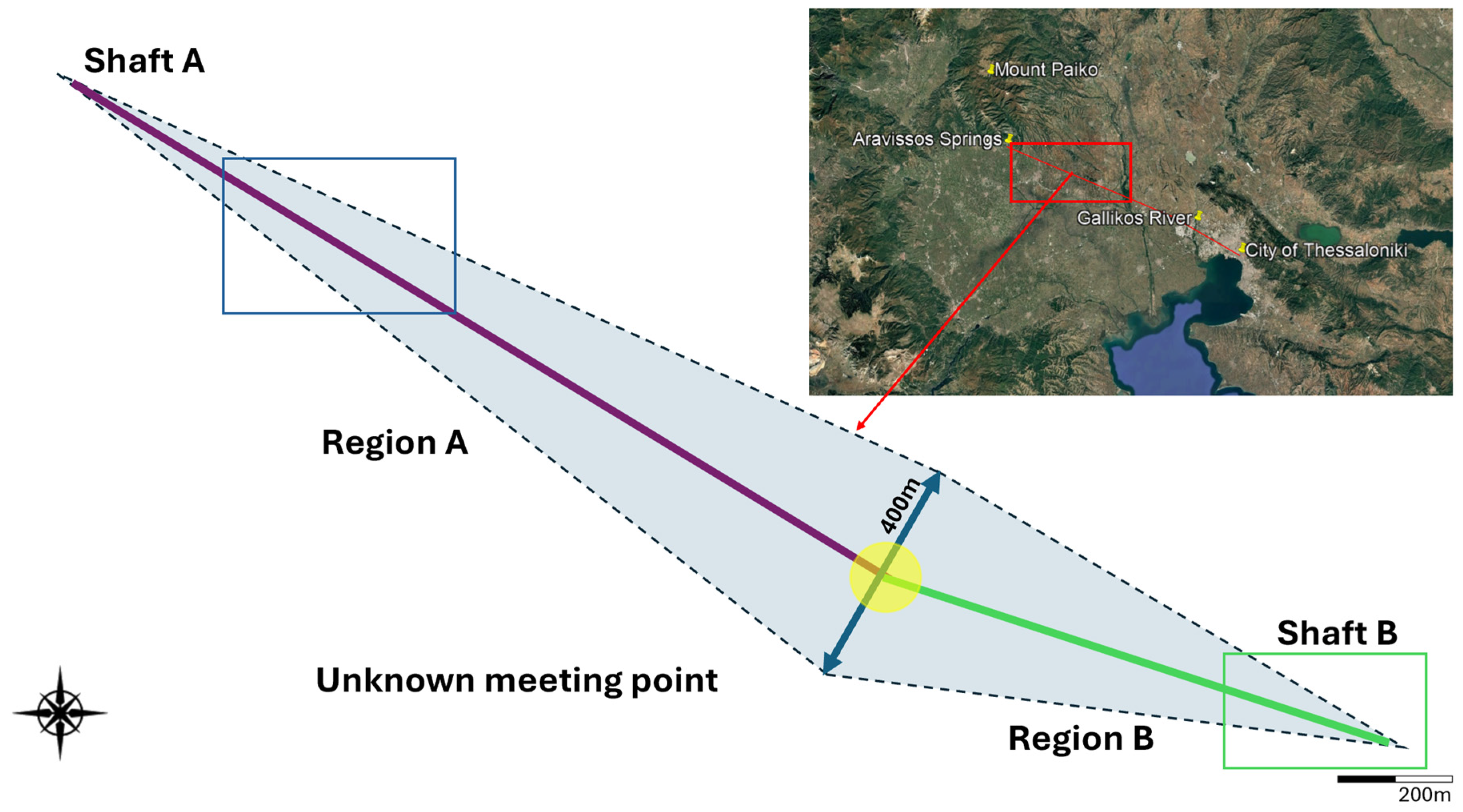
2.1. Description of Study Area and Use Case

The Aravissos pipeline, constructed between 1975 and 1978, spans approximately 52 km (51,968 m) from the Aravissos aqueduct to the western embankment of the Gallikos River. Originating from Aravissos Springs at Mount Paiko (Figure 1), this gravity-fed pipeline, buried at a depth of 2 to 2.50 m with a diameter of 1650 mm, is made of prestressed concrete reinforced with helical and longitudinal steel. Serving as a primary conduit for water transportation to Thessaloniki, the pipeline meets approximately 35% of the city’s daily water needs. The rupture of the pipeline in 2018 left many areas of the city without regular water supply for three weeks, highlighting its critical importance within the city’s extensive water supply network.

The section of the Aravissos pipeline examined in this study extends approximately 1500 m and as schematically illustrated in Figure 1, comprises two segments—Region A and Region B—originating from existing shaft structures identified through field surveys and archival documentation. The configuration shown in this diagram reflects the legacy pipeline alignment as depicted in outdated technical drawings prior to the present investigation. However, the precise direction remains uncertain, forming a critical ambiguity zone in their convergence region indicated by the yellow circle (Figure 1). The magenta and green lines represent the presumed pipeline axes derived from each region from the legacy maps, but field crews were unable to verify their exact position due to discrepancies in the historical data. The red line in the inset map denotes the approximate pipeline route extending from Aravissos Springs to Thessaloniki, providing a broader geographical context for the study area. This operational need provided the motivation for applying the multi-source remote-sensing workflow presented in this study.

It is important to note that due to the sensitive nature of critical water pipeline infrastructure, national security regulations (e.g., EU Directive 2022/2557 [33]; Law 5054/2023 [34]) and best practices for asset protection prohibit the public release of exact geographic coordinates or detailed imagery that could lead to precise localization of the infrastructure. Consequently, all spatial analyses were performed in a local plane whose origin was translated by an undisclosed constant offset.

2.2. NIR Aerial Survey Campaigns

To examine whether near-infrared (NIR) imaging could show an indication for the pipeline location, a DJI Mavic 3 NIR (SZ DJI Technology Co., Ltd., Shenzhen, China) drone was used. The imaging bands included green (G), 560 ± 16 nm, red (R), 650 ± 16 nm, red edge (RE), 730 ± 16 nm, and near infrared (NIR), 860 ± 26 nm. Flights occurred on clear days between 10:00 AM and 1:00 PM to maximize solar radiation and to minimize shadow effects from vegetation, with a flight altitude of 90 m, yielding RGB images with a 5 cm spatial resolution. The flight paths were pre-programmed using the DJI Pilot software (v 6.1.2), with a side overlap of 80% and a front overlap of 80%. Each flight took approximately 35 min, capturing 300 images per campaign. Eight aerial surveys were conducted between January 2024 and March 2025 to examine how vegetation cover and soil conditions influenced the detectability of subsurface features. These campaigns took place on 31 January 2024, 7 February 2024, 15 June 2024, 5 November 2024, 27 November 2024, 29 January 2025, 25 February 2025, and 22 March 2025. Images were georeferenced using the EGSA (Hellenic Geodetic Reference System 1987) 1987 system, with RTK applied for GNSS error correction. The images were processed with the Terra DJI software (v. 4.1.0) and further analyzed using ArcGIS Pro.

The analysis of the NIR images included the Normalized Difference Vegetation Index (NDVI) and the Optimized Soil-Adjusted Vegetation Index (OSAVI), which have been widely used to evaluate plant health and soil properties [35,36] and are shown in Equations (1) and (2):

$$\mathrm{N}\mathrm{D}\mathrm{V}\mathrm{I}={\displaystyle \frac{\mathrm{N}\mathrm{I}\mathrm{R}-\mathrm{R}\mathrm{e}\mathrm{d}}{\mathrm{N}\mathrm{I}\mathrm{R}+\mathrm{R}\mathrm{e}\mathrm{d}}}$$

(1)

$$\mathrm{O}\mathrm{S}\mathrm{A}\mathrm{V}\mathrm{I}=1.16{\displaystyle \frac{\mathrm{N}\mathrm{I}\mathrm{R}-\mathrm{R}\mathrm{e}\mathrm{d}}{\mathrm{N}\mathrm{I}\mathrm{R}+\mathrm{R}\mathrm{e}\mathrm{d}+0.16}}$$

(2)

The NDVI threshold of 0.35, used for pipeline trace delineation, was determined through iterative analysis of our multi-temporal dataset. This threshold was selected based on three criteria: (1) seasonal optimization—during optimal detection periods (early regrowth phases with NDVI ≈ 0.30–0.45), pipeline-induced vegetation stress consistently manifested as values below 0.35, while surrounding healthy vegetation exceeded this threshold; (2) visual validation against true-color imagery confirmed that 0.35 effectively separated visible linear anomalies from background vegetation in our Mediterranean agricultural setting; and (3) sensitivity analysis across alternative thresholds (0.30 and 0.40) showed 0.35 provided optimal balance between detection sensitivity and false-positive suppression. This threshold selection approach ensures reproducibility while acknowledging that site-specific calibration may be required for different vegetation types and climatic conditions.

All raster layers were processed in ArcGIS Pro and rendered with fixed symbology so that identical colors correspond to identical index values across the entire time-series. True-color imagery was displayed with a standard 8-bit linear stretch. NDVI layers were rendered using a percent-clip stretch from 0.75 (red) to 0.80 (green) with a gamma of 0.5. OSAVI layers, calculated as 1.16*(NIR–red)/(NIR + red + 0.16), and were rendered with a minimum–maximum stretch from –0.13 (pale violet) to 0.23 (deep violet) with a gamma of 1.2. All stretch types, range limits, and gamma values were held constant for each of the campaign dates.

2.3. Sentinel-2 Data

The satellite data used in this study were obtained from the Sentinel-2 (S-2A) satellite for soil monitoring purposes. The georeferenced data were accessed from the Copernicus Data Space Ecosystem [37]. Sentinel-2 (S-2A) carries a multispectral instrument (MSI) that acquires reflected solar radiance in 13 bands between 440 and 2200 nm spectral wavelength (Esa, 2018). The spatial resolution was 10 m for the red, green, blue, and near-infrared bands; 20 m for six more bands in the NIR (705–865 nm) and short-wave infrared (SWIR, 1600–2200); and 60 m for three other bands (443, 940, and 1375 nm). Sentinel-2 (S-2A) satellite orbits have a 5-day revisit time in paired operations, with image acquisitions taking place around 9:29 UTC (Coordinated Universal Time) (i.e., 11:29 and 12:29 local time in winter and summer, respectively). Level-2A processing includes a Scene Classification and an Atmospheric Correction applied to Top-Of-Atmosphere (TOA) Level-1C orthoimage products. The main output of Level-2A processing, which has been used in this study, is an atmospherically corrected orthoimage Surface Reflectance product.

2.4. Google Earth

Using Google Earth Pro’s “Historical Imagery” slider, the pipeline track on the ground proved distinctly visible on only three occasions—5 August 2002, 11 June 2011 and 14 July 2011—out of a total of 17 available acquisition dates for the study area. At a fixed zoom level (ground sampling distance ≲ 0.5 m), full-resolution screenshots of these three dates were exported, then imported into ArcGIS Pro and warped to the EGSA 1987 (EPSG:2100) projection. Georeferencing relied on at least five visually identified ground control points—road intersections, field edges, and surveyed shaft locations.

Table 1. Summary of remote-sensing data sources, specifications, and derived products.

Data Source	Spatial Resolution	Spectral Bands	Temporal Coverage	Key Products	Positional Accuracy
UAV (DJI Mavic 3 NIR)	5 cm	G (560 ± 16 nm), R (650 ± 16 nm), RE (730 ± 16 nm), and NIR (860 ± 26 nm)	8 campaigns (Jan 2024–Mar 2025)	NDVI and OSAVI	±0.30 m
Sentinel-2	10 m (VNIR), 20 m (RE/SWIR), and 60 m (atmospheric)	13 bands (440–2200 nm)	221 scenes (2015–2020)	Soil discoloration maps and false-color composites	±13.0 m
Google Earth	~0.5 m	RGB (visible spectrum)	3 dates (2002 and 2011)	Orthophotos and soil/vegetation marks	±1.0 m
Traditional methods, GPR *	<1 m lateral	N/A	N/A	Depth profiles	±0.1–0.5 m
Legacy maps	N/A	N/A	1975–1978	Pipeline routes	Up to 300 m error

* Ground-Penetrating Radar.

summarizes the diverse remote-sensing platforms employed in this study, highlighting the trade-offs between spatial resolution, temporal frequency, and positional accuracy. The multi-sensor approach leverages each platform’s strengths: a UAV’s centimeter-scale resolution for detailed vegetation analysis, Sentinel-2′s high temporal frequency for change detection, and Google Earth’s historical archive for temporal baseline establishment.

2.5. Data Analysis and Error Evaluation

Surface-expression anomalies associated with the buried pipeline were independently delineated in each remote-sensing dataset and then integrated through a unified least-squares workflow consisting of three stages: (1) feature extraction, (2) axis determination, and (3) uncertainty quantification. Concerning feature extraction and the NIR drone imagery, fixed thresholds were applied to RGB, NDVI, and OSAVI rasters to highlight vegetation- and soil-related anomalies. We manually digitized the two boundaries of each water pipeline-related anomaly in a GIS as polylines, ensuring the vertices followed the visible edges of the spectral contrast. As for the Sentinel-2 images, NIR–red–green false-color composites were screened for continuous pale bands aligned with the expected pipeline traces on the soil surface. Each detected discoloration area was visually traced as a closed GeoJSON (Geographic JavaScript Object Notation) polygon (repeated 3 times). For the Google Earth photos, each anomaly was digitized three times to capture operator variability; the resulting screenshots were georeferenced using ≥ 5 ground control points. For axis determination, every individual vertex along all digitized anomaly lines—the coordinate points defining trench edges or soil-discoloration bands—was projected into a local Cartesian system (EGSA 1987, EPSG (European Petroleum Survey Group): 2100) with the shafts fixed as the origin. A single, average centerline was then obtained for each dataset by fitting a least-squares regression, constrained to pass through the shafts’ coordinates, to the entire vertex cloud. The best-fit linear axis, representing the mean orientation of the traced pipeline feature, was obtained by solving a constrained orthogonal least-squares regression (minimizing the sum of squared perpendicular distances of all digitized vertices to a line forced through the reference shaft) and then exported as KML (Keyhole Markup Language) for seamless GIS integration. Positional uncertainty for each sensing method was quantified by combining three independent error components in quadrature:

$$E_{total}=\sqrt{E_{scatter}^2+E_{geo}^2+E_{dig}^2}$$

(3)

where each component represents fundamentally different uncertainty mechanisms:

• E_scatter quantifies the spatial dispersion of traced features and reflects natural variability in surface expression width and continuity;
• E_geo represents platform-specific horizontal geolocation accuracy derived from technical specifications (RTK GNSS for UAV: ±0.03 m; Sentinel-2 metadata: ±12.5 m; and Google Earth georeferencing: estimated ±0.5 m based on ground control point residuals);
• E_dig captures operator variability through triplicate digitization analysis.

This root-sum-square combination assumes Gaussian error distributions and statistical independence between sources—assumptions validated through comparisons with RTK-GNSS ground truth measurements. The methodology described above delineated the potential operational areas for the survey crews to locate the buried pipeline. Guided by these results, an exploratory trench measuring 7 m in length, 1.5 m in width, and 2.5 m in depth was excavated through the projected junction zone. The exposed pipeline crown was surveyed using a Spectra Geospatial SP85 RTK-GNSS receiver in order to establish a ground-truth centerline. Simultaneously, a DJI Mavic 3 M unmanned aerial vehicle was flown in a tightly spaced grid pattern over the trench, and the resulting high-resolution images were processed to produce an orthophotograph of the excavation site. All ground-truth data and orthophotographs were imported into ArcGIS Pro, together with the UAV, Sentinel-2, and Google Earth data layers, to facilitate a comprehensive comparative analysis of positional discrepancies. The quantification of errors is shown in

Table 2. Quantification of error components and their relative contributions to total positional uncertainty.

Method	Escatter (m)	Egeo (m)	Edig (m)	Etotal (m)	Dominant Error Source (%)
UAV-NIR	0.29	0.03	0.05	±0.30	Scatter
Sentinel-2	4.5	12.5	2.0	±13.0	Geolocation
Google Earth	~0.8 *	~0.5 *	~0.3 *	±1.0	Scatter

* Estimated values based on total error and typical proportions.

.

3. Results

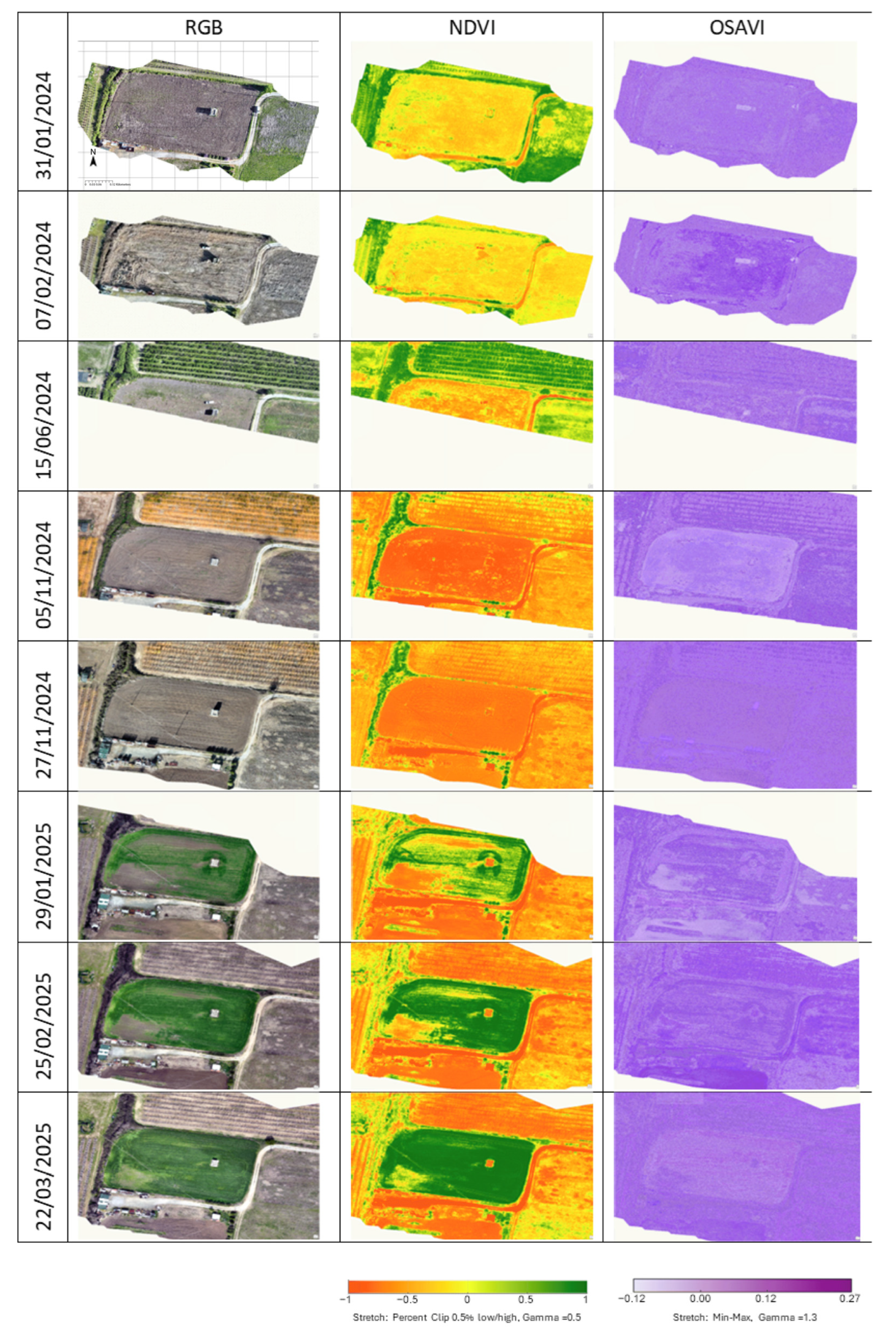
3.1. Data Acquisition from UAVs

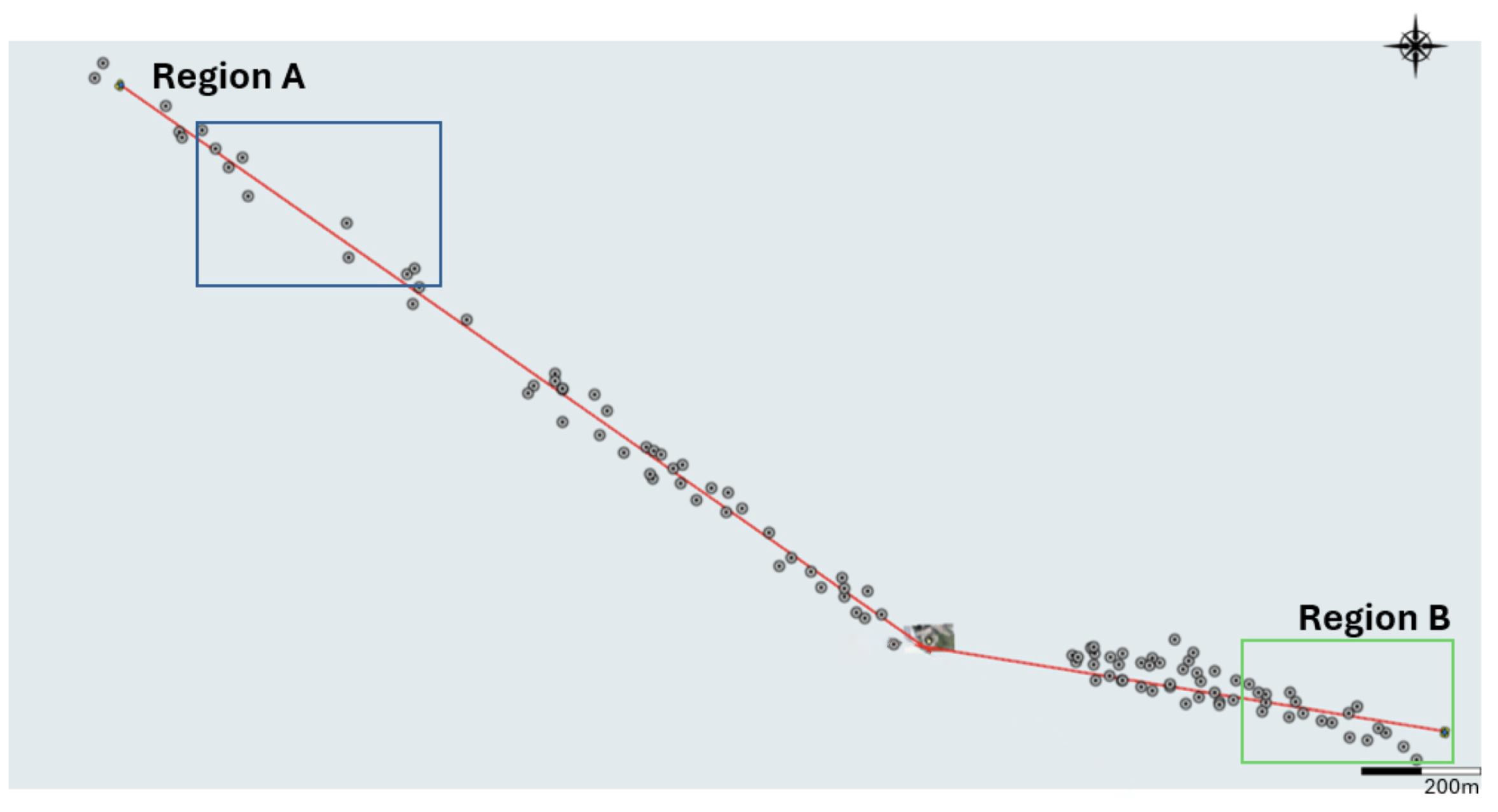
3.1.1. Identifying the Pipeline Traces with UAVs

Figure 2 shows the true-color (left), NDVI (center), and OSAVI (right) imagery of the study field at Region A (as shown by the blue rectangle in Figure 1) on 31 January 2024, 15 June 2024, 5 November 2024, 27 November 2024, 29 January 2025, 25 February 2025, and 22 March 2025, all rendered with fixed symbology (NDVI 0.75–0.80, γ = 0.5; OSAVI –0.13–0.23, γ = 1.2). Specifically, on 31 January 2024, beneath dense vegetation, while the NDVI signal is largely saturated at its high end across the field, a very faint trace of the buried pipeline alignment can nevertheless be discerned upon close inspection within the NDVI imagery. OSAVI, however, fully saturates into deep violet on this date, making the alignment indistinguishable in that particular index. By 15 June 2024—immediately post-harvest—the residue distribution and soil compaction along the back-filled trench can be seen in true color as a very subtle tonal stripe, yet neither NDVI nor OSAVI shows any anomaly. Both indices have collapsed to their low-end values (NDVI < 0.15; OSAVI ≈ 0.00) and lack the dynamic range to discriminate the subsurface water infrastructure trace. On 5 November 2024, NDVI remains low (≈0.18–0.20) and featureless, but OSAVI faintly highlights the water pipeline trace as a pale-violet band (mean OSAVI ≈ 0.05 inside vs. 0.12 outside the trench). By 27 November 2024, no traces of the pipeline are visible in any image. During early regrowth on 29 January 2025, both indices enter mid-range (NDVI ≈ 0.30–0.45; OSAVI ≈ 0.12–0.18) and each depicts the trench as a subdued stripe. By 25 February 2025, as the vegetation cover increases, NDVI (≈0.60–0.70) and OSAVI (≈0.20–0.30) both clearly delineate the pipeline, and even at peak greenness on 22 March 2025—when NDVI exceeds 0.75 and OSAVI exceeds 0.20—the alignment remains detectable as a faint linear anomaly.

The above observations reveal that in bare-soil or early vegetation conditions, OSAVI’s soil adjustment excels at highlighting possible pipe location indications. Once vegetation establishes (NDVI ≈0.30 and higher), NDVI generally provides good contrast. At peak biomass levels (NDVI > 0.75), detectability diminishes significantly: the pipeline appeared as a “faint linear anomaly” in both NDVI and OSAVI in March 2025. However, under the dense vegetation of January 2024, this feature was reduced to a “very faint trace” in NDVI, discernible only upon close inspection, while it became indistinguishable in the concurrently fully saturated OSAVI. This highlights the varying responses of different indices at high vegetation densities and the importance of considering potential saturation effects and the limits of visual interpretation. Threshold sensitivity analysis confirmed the robustness of our NDVI = 0.35 selection: testing alternative values of 0.30 and 0.40 resulted in either excessive noise inclusion (0.30) or incomplete trace capture (0.40), respectively. The selected threshold maintained consistent detection across our eight-mission temporal series while minimizing false positives from natural vegetation variability.

Figure 3 shows true-color (left), NDVI (center), and OSAVI (right) imagery at Region B (shown in Figure 1 with the green rectangle) over the same seasonal sequence as Figure 2—plus a second spring revisit—rendered with identical symbology (NDVI 0.75–0.80, γ = 0.5; OSAVI –0.13–0.23, γ = 1.2). Across all eight dates, the buried pipeline alignment remains completely undetectable. On the bare-soil and post-harvest dates (31 January 2024 and 15 June 2024), the RGB mosaics are uniformly pale; NDVI falls below 0.15 (deep red–orange) and OSAVI to ≈ 0.00 (pale violet), erasing any trace of subsurface disturbance. During the late-autumn flights (5 November and 27 November 2024), NDVI rises only to ≈ 0.18–0.20 and OSAVI to ≈ 0.05–0.10, yet both indices still portray a homogeneous field with no linear anomaly. With early regrowth on 29 January 2025, NDVI (≈0.30–0.50) and OSAVI (≈0.10–0.20) begin to differentiate orchard rows from bare patches, but the pipeline trace does not emerge. Finally, once the vegetation completely covers the soil (25 February 2025; NDVI ≈ 0.60–0.70; OSAVI ≈ 0.20–0.30) and peak greenness (22 March 2025; NDVI > 0.75; OSAVI > 0.20), the entire plot saturates into uniform green and violet, and the subsurface alignment remains invisible.

The observed vegetation-index responses are underpinned by the biophysical effects of subsurface soil disturbance. Altered soil properties in back-filled trenches (e.g., compaction and modified porosity) induce localized moisture gradients that stress overlying vegetation—a principle established in archaeological prospection [38,39] and for detecting stress above buried structures, even from slight leaks [1,7]. Supporting these mechanisms, recent research demonstrates the reliability of vegetation-stress indices for locating pipeline leaks and the efficacy of soil-adjusted metrics, like OSAVI, in capturing moisture-brightness contrasts under sparse cover [40]. Furthermore, long-term studies show that trench-induced compaction and root-zone damage persistently suppress canopy vigor, measurable via broad-band indices, such as NDVI [41]. Consistent with this body of literature, our results affirm that a phenology-driven integration of OSAVI and NDVI optimizes UAV-based surveys, enabling robust and repeatable detection of buried pipeline traces across seasonal vegetation cycles.

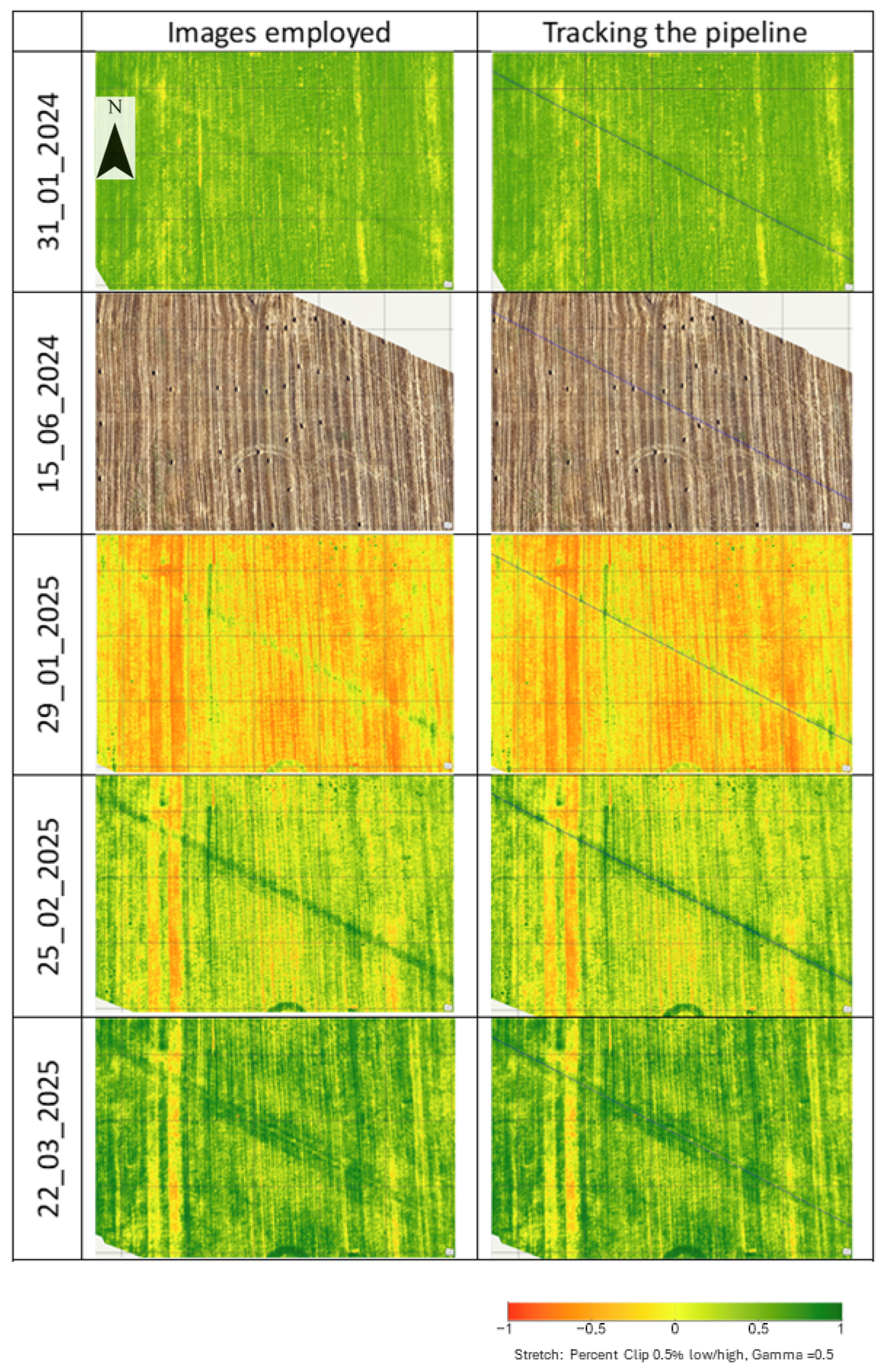
3.1.2. Marking the Traces with UAVs

Figure 4 (left column) shows four NDVI images (31 January 2024, 29 January 2025, 25 February 2025, and 22 March 2025) displayed with consistent symbology, alongside one true-color RGB orthomosaic (15 June 2024). These images from Region A illustrate how the buried pipeline’s visibility in spectral data changes seasonally. In the right column, blue lines mark the pipeline soil trace margins, manually digitized from each NDVI image using pixels with NDVI values below 0.35. The 15 June 2024 RGB image, which shows low contrast in vegetation indices, was interpreted visually to delineate the trench trace. All digitized lines were anchored at their upstream end to the surveyed position of shaft A. As detailed in Section 2.5, these individual trench traces were then processed to calculate a single average pipeline axis from the UAV data. This involved projecting all vertices into a local Cartesian system originating at shaft A and fitting a constrained least-squares regression through the combined points. The resulting best-fit axis represents the mean orientation of the UAV-derived traces (Figure 4), with a horizontal uncertainty of ±0.30 m. This uncertainty was calculated by combining three error sources in quadrature: inter-trace variability (0.29 m), GNSS georeferencing errors (0.03 m), and manual digitization errors (0.05 m). In contrast, this NDVI thresholding approach did not detect a continuous linear anomaly in Region B using UAV data. Consequently, Sentinel-2 imagery was subsequently used to assess detectability at a broader scale.

3.2. Data Acquisition from Sentinel-2

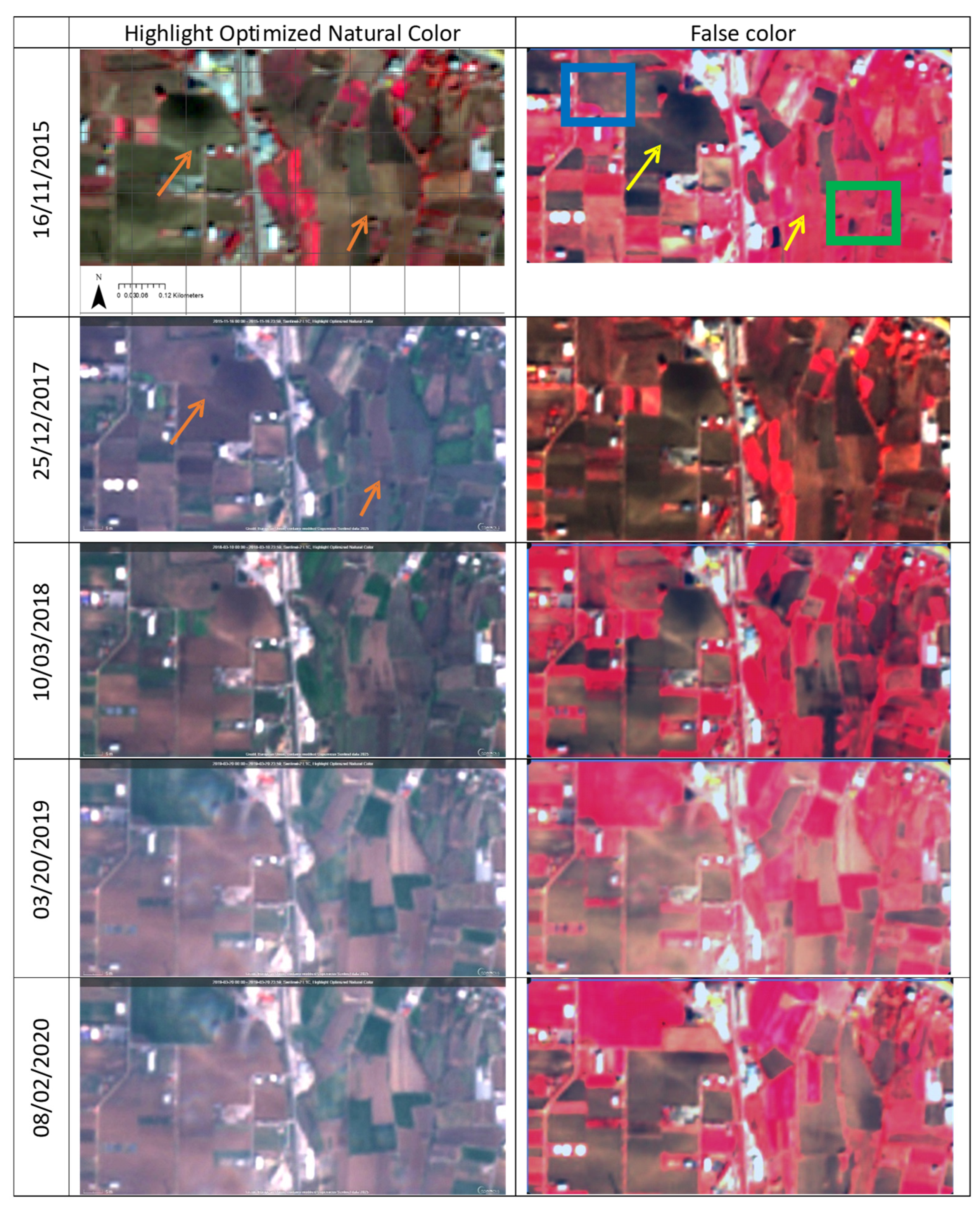
3.2.1. Identifying Pipeline Traces with Sentinel-2

Figure 5 presents a series of indicative Sentinel-2 L1A (Level-1A (Sentinel-2 Product Level)) scenes—chosen to be representative of the timeframes when the buried pipeline trace can be tracked both in Regions A and B using 10–20 m Sentinel-2 data—displayed in true-color (left) and NIR–red–green false color (right). The blue and green boxes mark the A and B regions previously surveyed by a drone, and orange arrows in the true-color panels alongside yellow arrows in the false-color images pinpoint the faint soil bands corresponding to the trench alignment. False-color composites were generated by mapping bands B08 (NIR), B04 (red), and B03 (green), with a channel gain of 2.5, a gamma correction of 1.2, and stretch limits set to red = 0.32–1.00, green = 0.13–1.00, and blue = 0.21–0.83; these adjustments enhance subtle differences in soil color, rendering the pale disturbance zones more discernible.

• In the 16 November 2015 scene, the unplanted field appears uniformly brown in true color, yet the orange arrows draw attention to two nearly imperceptible pale lines cutting diagonally through the field—one downslope of shaft A, the other just southwest of shaft B. The false-color composite renders these same features as narrow, cool-tone streaks, with the yellow arrows, indicating reduced NIR reflectance.
• By 25 December 2017, orange arrows still trace a faint linear pattern near shaft A. In the NIR composite, this trench line persists as a delicate low-NIR band (yellow arrow), whereas shaft B shows a coherent pale anomaly.
• The 10 March 2018 acquisition captures early spring green-up, and the true-color image’s orange-arrowed alignment is now masked by emerging vegetation. Likewise, the false-color panel—highlighted by yellow arrows—displays a continuous linear feature.
• On 20 March 2019, satellite images again reveal soil tone variations. Here, an orange arrow in the true-color composite marks a pale line southeast of shaft A, while the false-color image accentuates this band (yellow arrow) as a distinct low-NIR track, whereas near shaft B, the trace is not observable.
• Finally, the 8 February 2020 scene shows both orange and yellow arrows which indicate where the pipeline alignment would lie.

Sentinel-2 satellite imagery consistently reveals distinct, broad linear soil discoloration patterns indicative of the buried pipeline infrastructure, particularly evident in post-harvest (e.g., 16 November 2015 and 25 December 2017), bare soil (e.g., 8 February 2020), and early-spring (e.g., 10 March 2018 and 20 March 2019) scenes. These features, typically spanning 15–30 m in width and resolved by Sentinel-2′s 10–20 m spatial resolution, significantly exceed the actual pipeline trench dimensions. They predominantly reflect widespread alterations in soil optical properties—such as moisture retention and textural contrasts—rather than direct, localized vegetation stress. The substantial lateral extent of these discolorations suggests their genesis is not solely attributable to the immediate physicochemical properties of the backfill material. Instead, these broad surficial expressions are hypothesized to arise from complex, long-term interactions between the pipeline system and the encompassing hydrogeological, biogeochemical, and geomechanical environment.

The development of these extensive features results from multiple interacting mechanisms that modify soil properties well beyond the immediate trench footprint. Three primary processes drive these modifications: (1) hydrological alterations from contrasting hydraulic properties between backfill and native soil [41]; (2) geochemical changes, including salt migration and oxidation processes; and (3) physical modifications from construction-related soil compaction. Additionally, decades of agricultural practices have enhanced the surface expression of these subsurface disturbances. The following sections detail how each mechanism contributes to the broad spectral signatures observed in Sentinel-2 imagery, contrasting with the narrower vegetation stress patterns detected by UAV surveys.

Detailed Physical Mechanisms

To better understand these processes, it is instructive to consider parallels with archaeological remote sensing, where similar soil discoloration patterns have been extensively documented. Archaeological research has shown that buried anthropogenic features—whether ancient ditches or modern pipelines—create persistent spectral anomalies through fundamentally similar mechanisms [42]. This body of research provides valuable insights for interpreting our pipeline signatures, as both contexts involve linear buried features with contrasting infill properties that modify overlying soil characteristics. Drawing on these archaeological principles while considering the specific properties of pipeline construction, we can identify several key mechanisms:

Water Migration: Pipeline trenches fundamentally alter subsurface hydrology through three key processes. First, the backfill–soil interface creates preferential flow paths where water accumulates during precipitation, following the pipeline alignment [41]. Second, particle size differences between backfill and native soil generate capillary barriers that force lateral water redistribution, expanding the detectable anomaly width to 15–30 m despite narrower trench dimensions [11,15]. Third, compacted trench bases create perched water conditions, maintaining elevated moisture in overlying soil. These moisture variations are particularly detectable in Sentinel-2′s NIR band (B08: 842 nm) and visible bands where wet soil appears darker [8,31].

Salt Accumulation: In our semi-arid study area, evapotranspiration drives upward salt migration, with pipeline trenches acting as collection zones for dissolved minerals. During dry periods, capillary rise brings salts to the surface where they crystallize, creating high-albedo features visible in Sentinel-2′s blue (B02: 490 nm) and green (B03: 560 nm) bands. This process intensifies along pipelines due to enhanced lateral groundwater flow toward the disturbed zone [8].

Agricultural Enhancement: Consistent with archaeological observations [13,42], repeated plowing significantly enhances pipeline visibility by progressively mixing deeper backfill material with surface soil. Modern deep plowing (20–30 cm) brings contrasting soil to the surface, while differential erosion between compacted and loose zones creates microtopographic variations [23]. These effects are most pronounced in our post-harvest (November–December) and late-winter (February–March) imagery when bare soil maximizes contrast.

Temporal Persistence: Unlike vegetation anomalies that vary seasonally, these soil marks demonstrate remarkable persistence across our 2015–2020 observations. This “soil memory” effect results from permanent modifications to soil structure and chemistry during pipeline installation [10,25]. The lateral expansion of these features, through the mechanisms described above, creates broad zones detectable at Sentinel-2′s 10–20 m resolution, providing reliable indicators for pipeline mapping despite the sensor’s moderate spatial resolution.

3.2.2. Marking the Traces

Figure 6 presents the estimated pipeline alignment as derived from multi-date Sentinel-2 imagery. For each selected scene from Figure 5, pale-soil discoloration patterns were manually outlined, and the boundary vertices of these polygons—shown as grey circles—were used as input for linear regression. Following the method described in Section 2.5, a least-squares axis was computed for each segment, constrained to pass through the respective shaft. The Sentinel-based method identified the pipeline traces in both regions, and their intersection defines the most likely junction between the northern and southern pipeline paths. Positional uncertainty was quantified by combining the root-mean-square scatter of the polygon vertices relative to each regression line (E_scatter ≈ 4.5 m), Sentinel-2′s geolocation error (E_geo = ±12.5 m), and digitization variability (E_dig ≈ 2 m), resulting in a one-sigma total error of approximately ±13.0 m. While this is coarser than UAV-based mapping, Sentinel-2 imagery remains useful for broader-scale detection in areas lacking drone coverage, such as Region B.

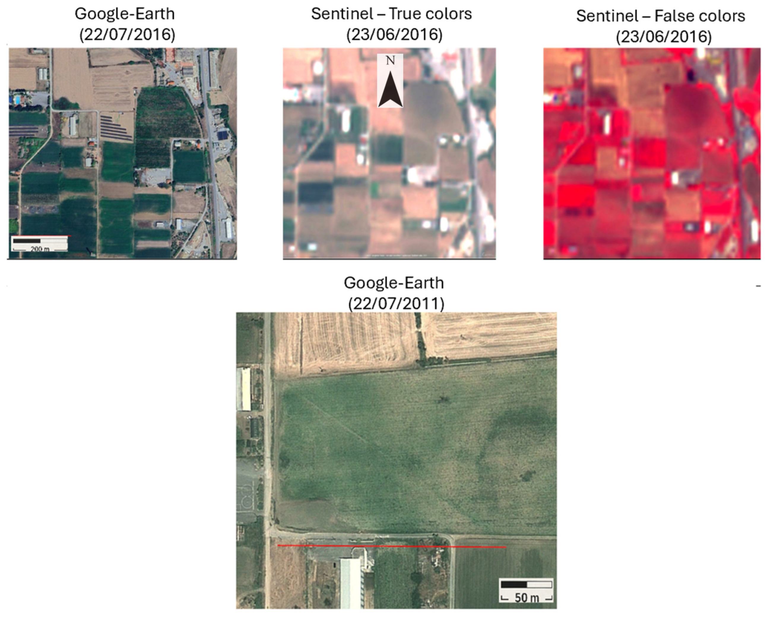
3.3. Data Acquisition from Google Earth

We processed Google Earth orthophotos from 5 August 2002, 11 June 2011, and 14 July 2011 using the same least-squares workflow as the UAV and Sentinel-2 datasets. For each date, the visible soil–vegetation disturbance was digitized three times, all vertices were reprojected to EGSA 1987 (EPSG:2100), and an orthogonal least-squares regression, constrained through the shaft coordinate, was fitted to each dataset cloud. The three date-specific axes (slopes and intercepts) were then averaged to produce a single, 2 km reference centerline for the Google Earth dataset. Positional uncertainty for this averaged axis was computed by combining, in quadrature, the vertex scatter RMSE (root-mean-square error, E_scatter), the affine-georeferencing error (E_geo), and the digitization repeatability (E_dig), yielding σ_total ≈ 1 m (1 σ).

Figure 7 compares visual evidence of an underground pipeline’s surface expression using two distinct remote-sensing datasets from comparable dates: high-resolution Google Earth imagery (22 July 2011 and 22 July 2016) and Sentinel-2 imagery (23 June 2016, presented as true- and false-color composites). Both datasets effectively identify the broad linear features corresponding to the pipeline’s route. The image dates were selected based on the optimal clarity of these pipeline-related surface anomalies in both data sources within a similar temporal window. The pipeline’s surface manifestation is observable through at least two distinct effects: (1) fine-scale variations in vegetation, often appearing as linear patterns of growth or stress, and (2) soil discoloration. Notably, the detectability of these phenomena varies with the sensor. Vegetation variations are more clearly discernible in the high-resolution Google Earth imagery, consistent with previous UAV-based near-infrared (NIR) observations. Conversely, soil discoloration is adequately visible in both Google Earth and the coarser resolution Sentinel-2 data. It is posited that both trace types are secondary effects of the buried infrastructure. However, the specific physical or chemical mechanisms driving the vegetation anomalies versus the soil chromaticity changes likely differ. Elucidating these causal links is beyond the scope of this study but represents an area for future research. To our knowledge, no published studies have directly compared these dual manifestations across these specific remote-sensing platforms.

4. Discussion

This study evaluated an integrated remote-sensing framework for pipeline detection and localization, particularly in contexts where legacy mapping is absent or unreliable. The discussion below synthesizes the findings, addresses methodological strengths and limitations, and considers the practical implications of the results.

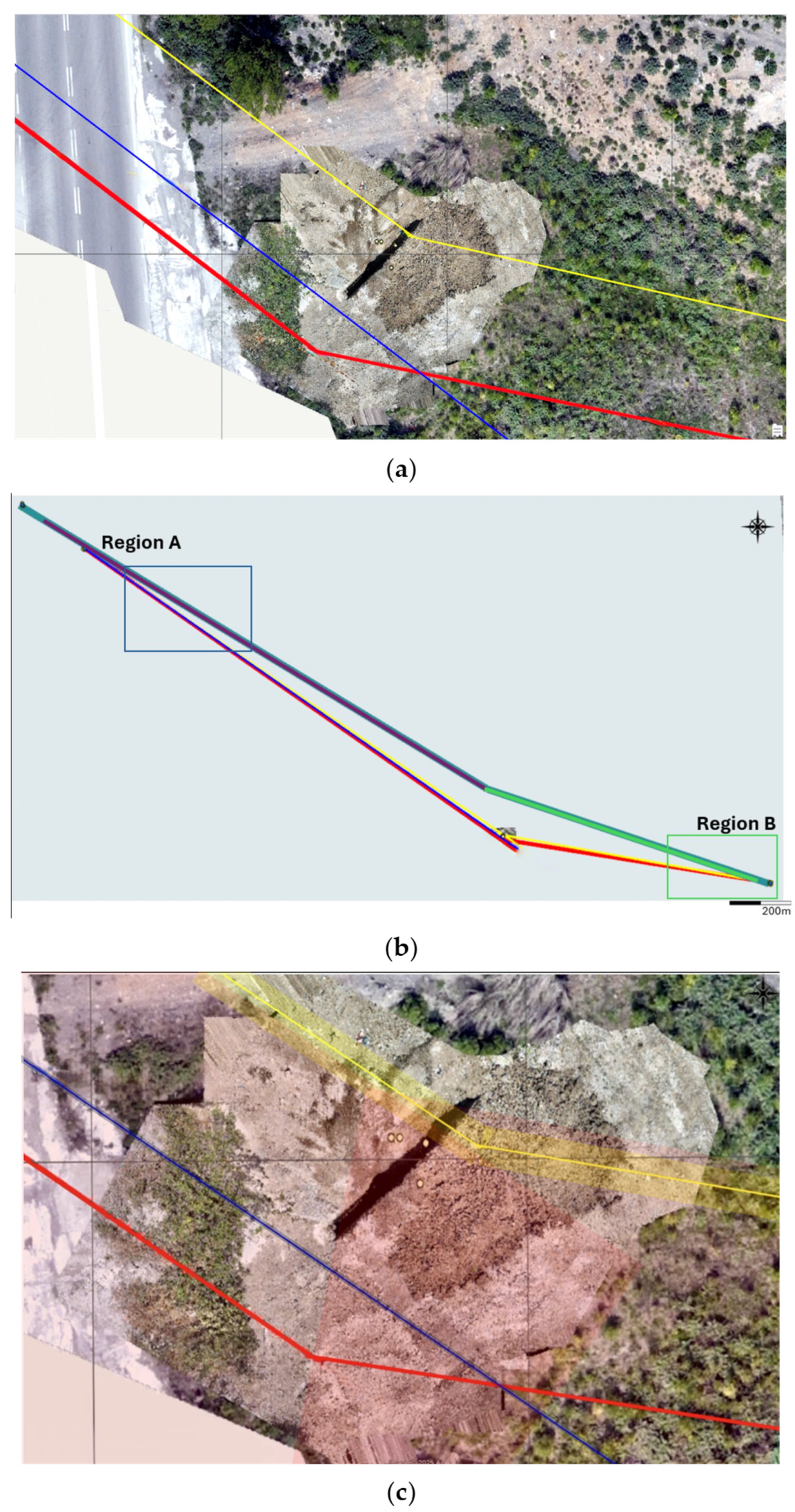
4.1. Comparative Analysis of Pipeline Alignments and Efficacy of Remote Sensing

An integrated comparison of pipeline alignments derived from the different methodologies is presented in Figure 8. Specifically, Figure 8a illustrates the pipeline alignments generated from three distinct remote-sensing analyses: (a) unmanned aerial vehicle (UAV)-based vegetation indices (Normalized Difference Vegetation Index, NDVI; Optimized Soil-Adjusted Vegetation Index, OSAVI), (b) historical Google Earth orthophotography, and (c) Sentinel-2 multispectral satellite data. These are juxtaposed with the original legacy pipeline map. The high-resolution UAV imagery acquired over Region A enabled the calculation of a precise pipeline axis (dark-blue line). The pipeline axis derived from multi-temporal Google Earth orthophotos is depicted in yellow, while the Sentinel-2-derived axis is shown in red. The intersection of these latter two datasets provided an initial estimate of the pipeline junction. The original “legacy” pipeline alignment is represented by magenta and green colors.

A key observation from Figure 8a is the substantial congruence in the derived pipeline alignments from all three remote-sensing modalities (UAV, Google Earth, and Sentinel-2). This mutual agreement underscores the collective accuracy of the remote-sensing approaches. Conversely, the legacy mapping demonstrates a marked divergence, positioning the putative junction point of the two pipeline segments several hundred meters from the location identified by the contemporary remote-sensing analyses. This discrepancy highlights the utility of the proposed multi-sensor remote-sensing framework, especially in rural environments where accurate cartographic information may be deficient. The hierarchical approach employed—the initial detection of broad soil-discoloration anomalies using medium-resolution satellite data (Sentinel-2), a refinement of surface patterns with high-resolution orthophotography (Google Earth), and a precise delineation of the pipeline trace through targeted UAV-borne near-infrared (NIR) vegetation index analysis—proved effective. Despite general agreement, a closer examination of the intersecting points suggested by each remote-sensing method reveals discrepancies in the order of several meters. Figure 8b provides orthophotographic details of the potential intersection site. The shaded bands enveloping the axes derived from each method represent the quantified total positional uncertainty (E_total), while divergence is further emphasized in the magnified view presented in Figure 8c.

4.2. Excavation Strategy, Validation, and Operational Implications

The observed discrepancies in junction point estimations raise a pertinent practical question: how should excavation be guided based on such multi-source information? Considering the calculated positional accuracies, prioritization of the UAV-NIR data (±0.3 m) would appear logical. However, the efficacy of the NIR method is highly contingent upon specific surface conditions, including soil type, moisture content, and, critically, the density and phenological state of the vegetation cover. A preliminary NIR survey is often advisable to assess its suitability for pipeline detection under site-specific conditions, as a continuous and unambiguous signal along the entire pipeline trajectory, particularly at intersections, is not always guaranteed. In this investigation, while the NIR method yielded a distinct signal along segments of the pipeline, signal discontinuity or ambiguity within the critical intersection zone prevented the identification of a precise crossing point using this method exclusively. Consequently, excavation was initiated proximate to the intersection suggested by the next most accurate method, Google Earth (±1 m accuracy). The trench, with a width of 1.5 m, was oriented towards the broader zone of interest indicated by the NIR data (Figure 8c). Given that approach, the southern pipeline segment (Region B) was successfully located approximately 0.4 m from the Google Earth-derived position (the located pipe’s path is indicated by yellow GPS-recorded points). It is imperative to acknowledge a potential confirmation bias: the discovery of the pipe near the Google Earth-indicated point, subsequent to targeting that area, does not definitively exclude the possibility that the NIR indication might have been equally or more accurate.

Despite the successful localization of the southern segment, the Google Earth-derived intersection point could not be definitively confirmed, and the northern pipeline segment was not identified within the initial excavation extent. For the specific utility work undertaken, the localization and confirmation of any accessible segment of the pipe fulfilled the immediate operational requirements; thus, further excavation to precisely locate the northern segment or the junction was not pursued. It is important to note that the full validation of the predicted junction point was hindered by site-specific logistical constraints. The suspected location of the junction, based on the remote-sensing analyses, appeared to be beneath an active roadway. The necessary permissions and logistical arrangements to excavate a public road were beyond the scope and immediate operational requirements of this particular utility intervention. This situation highlights a real-world challenge in applying such methodologies: while remote sensing can provide accurate predictions, final ground-truth validation can sometimes be limited by accessibility, land use, or infrastructure.

Moreover, it is important to emphasize that the methodology achieved its primary operational objective with high confidence. The successful location of the southern pipeline segment within 0.4 m of the Google Earth-derived position validates the accuracy of our multi-source approach. This outcome demonstrates that the integrated remote-sensing workflow provides sufficient precision for practical utility operations, reducing search areas from hundreds of meters (based on legacy maps) to sub-meter accuracy. The operational cost reduction of approximately 80% compared to extensive blind excavation or blanket geophysical surveys further validates the methodology’s practical effectiveness.

While the precise junction point was not located during this intervention, this did not compromise the operational requirements, as access to any pipeline segment was sufficient for the immediate maintenance needs. Should future operations require precise junction location, the dramatically reduced search area established by our methodology would enable targeted applications of complementary techniques. Ground-penetrating radar surveys along the confirmed pipeline alignments could locate the junction within the constrained zone defined by our remote-sensing analysis. The achieved validation—successfully locating the pipeline where predicted—demonstrates that our methodology provides the spatial accuracy required for operational decision-making, while establishing a framework for more detailed investigations when specific infrastructure features require precise locations.

4.3. Methodological Limitations

The combined remote-sensing approach, while advantageous, is subject to inherent limitations:

• The UAV-NIR (NDVI/OSAVI) method: Despite its high potential accuracy, this method demonstrated variable reliability. Its efficacy is highly sensitive to surface conditions (soil type, moisture, and vegetation characteristics). Beyond detection-related constraints, UAV surveys face significant operational limitations. Individual flights cover only 10–50 hectares, requiring multiple missions for extended pipeline networks with associated cost increases. Meteorological conditions severely restrict acquisition windows, as wind speeds exceeding 12–14 m/s, precipitation, or fog prevent operations, potentially eliminating entire optimal phenological periods. Battery constraints, limiting flight durations to 20–35 min, necessitate frequent interruptions.
• Google Earth imagery: The archival imagery in Google Earth, while invaluable, often has irregular and sometimes sparse temporal resolutions, particularly for specific rural locations. This makes it less reliable for systematic, continuous monitoring programs and more of an opportunistic data source when clear imagery coincides with optimal ground conditions. Successful detection is contingent upon favorable environmental conditions (e.g., minimal vegetation cover and optimal soil moisture to enhance discoloration), coinciding with the dates of image acquisition.
• Sentinel-2 multispectral data: Sentinel-2 provides valuable high temporal resolution (ca. 5-day revisit cycle), rendering its soil discoloration signal potentially useful for near real-time pipeline localization and monitoring of soil–pipe interactions. However, its utility is constrained by its comparatively low spatial resolution, resulting in a substantial positional uncertainty (±13.0 m).
• Site-specific validation constraints: The comprehensive validation of all predicted features, particularly complex ones, like pipeline junctions, may be impeded by practical on-the-ground limitations, such as the presence of existing infrastructure (e.g., roads) or restricted access, as encountered in this study.
• Temporal repeatability considerations: While this study successfully demonstrated the comparative accuracy of UAV (±0.3 m), Google Earth (±1 m), and Sentinel-2 (±13 m) data sources for pipeline detection, we acknowledge that a statistical analysis of data repeatability across seasons was not performed. Such an analysis would require extensive multi-temporal datasets collected across equivalent seasonal periods over multiple years.

Our preliminary observations reveal that vegetation conditions can vary significantly even between similar calendar dates in consecutive years (e.g., late January 2024 versus late January 2025), primarily due to variations in agricultural management practices, including planting schedules, irrigation regimes, and crop rotation patterns. These inherent variabilities in agricultural landscapes need to be carefully considered in any temporal repeatability study, potentially requiring collaboration with local farmers to document management practices.

Future studies focusing on temporal repeatability of pipeline detection should consider the following: (i) establishing a systematic multi-year data collection protocol across all seasons, (ii) documenting agricultural management practices and their timing, (iii) developing statistical models that account for both seasonal and agricultural-induced variability, and (iv) examining how different vegetation conditions affect the detectability of underground infrastructure. Such research would provide valuable insights into the optimal timing for data collection and the reliability of detection methods under varying environmental conditions.

A significant outcome of this multi-source approach is the establishment of a spatially explicit baseline of the pipeline’s surface signature. The temporal variability observed across different sensors and seasons underscores the importance of such a baseline. Future monitoring efforts can leverage this baseline; deviations from the established patterns—whether in vegetation indices from UAVs or soil discoloration patterns from Sentinel-2—could serve as early indicators of changing subsurface conditions, potentially signaling compromised pipeline integrity or active leakage. This proactive approach, moving from initial mapping to ongoing surveillance, is critical for preventative maintenance.

4.4. Proposed Workflow

The key findings of the present study confirm distinct contributions and optimal use cases for each data source:

• UAV-NIR Surveys: These provide the highest positional accuracy (±0.3 m, 1σ), pinpointing the pipeline via narrow vegetation stress anomalies. However, detection is contingent on specific phenological windows (e.g., post-sowing and early green-up), necessitating carefully timed acquisitions coordinated with local agricultural cycles.
• Sentinel-2 Imagery: This enables consistent, corridor-scale detection (±13.0 m, 1σ) through the identification of broader soil discoloration bands associated with long-term subsurface disturbance. Its high temporal frequency and wide-area coverage make it invaluable for initial screening and monitoring, despite its coarser spatial resolution.
• Google Earth Historical Imagery: This serves as a crucial bridge, offering meter-scale accuracy (≈±1 m, 1σ) for identifying both soil marks (comparable to Sentinel-2) and, opportunistically, finer vegetation patterns (approaching the detail of UAVs) when suitable archival imagery coincides with favorable ground conditions.

Based on the above validated capabilities, we propose the following operational sequence for practical applications:

• Initial Screening: Utilize a multi-temporal Sentinel-2 analysis (focusing on post-harvest and late-winter/early-spring scenes) to identify persistent pale-soil anomalies and delineate candidate pipeline corridors.
• Refinement: Consult historical high-resolution archives (like Google Earth) to refine the potential axis, leveraging images captured during periods of low vegetation cover.
• Precision Mapping: Deploy targeted UAV-NIR surveys during phenologically optimal windows to achieve centimeter-level centerline mapping immediately prior to excavation, maintenance, or repair activities.

This workflow not only provides significantly improved locational data, drastically reducing the search area compared to outdated records (by up to 300 m in our case study), but also furnishes asset managers with quantified uncertainty estimates for each stage, supporting risk assessment and providing a repeatable audit trail. While demonstrated on a concrete aqueduct in Greece, the methodology’s principles are readily transferable to other types of buried utilities and diverse environmental settings.

5. Conclusions

This study demonstrated that integrated multi-source remote sensing achieves substantial improvements in buried pipeline localization accuracy, reducing positional uncertainty from exceeding 300 m using legacy documentation to 0.3 m with UAV-based near-infrared surveys, approximately 1 m using Google Earth historical imagery, and 13 m employing Sentinel-2 multispectral data. The methodology successfully located a buried pipeline segment within 0.4 m of the remotely sensed prediction, validating the operational effectiveness of the approach. A search area reduction of 99.9 percent compared to legacy documentation translated to operational cost savings of approximately 80 percent through the elimination of extensive exploratory excavation. Optimal detection conditions were quantitatively established, with UAV-based vegetation indices performing most effectively within the NDVI range of 0.30 to 0.70, while Sentinel-2 soil discoloration signatures achieved maximum contrast during November through March acquisitions under minimal vegetation cover conditions. The developed methodology offers immediate practical applications for water utility operators engaged in maintenance planning and emergency response activities, where the rapid pipeline location directly impacts service restoration times and resource allocation. Infrastructure asset managers benefit from accurate spatial data for inventory updates, risk assessments, and interference analyses with proposed developments. Regulatory authorities gain enhanced capabilities for compliance monitoring and environmental protection through improved documentation of subsurface infrastructure. Engineering consultants can apply the workflow for pre-construction surveys, reducing project delays. The methodology’s transferability could be extended to alternative buried infrastructure, including gas distribution networks, telecommunication cables, and electrical conduits, with particular value in rural and semi-rural environments where historical documentation often proves inadequate or absent. Municipal planning departments can integrate the validated pipeline locations into geographic information systems for improved urban development coordination and emergency response planning.

Future research should focus on automating the data fusion and least-squares adjustment process within open-source GIS platforms, further investigating the specific soil-physical and chemical mechanisms underlying the observed Sentinel-2 discoloration patterns and exploring the potential of integrating hyperspectral or thermal UAV payloads to enhance detection capabilities, potentially enabling near real-time leak identification. Future research should also focus on a more detailed investigation of the distinct causal mechanisms behind the narrow, vegetation-related anomalies observed in high-resolution UAV imagery versus the broader soil discoloration patterns detected by satellite sensors. This could involve controlled field experiments, detailed soil sampling for physical and chemical analyses across pipeline transects, and integration with subsurface hydrological modeling to better understand the complex interactions between buried infrastructure and the overlying surface environment. Finally, assessing the temporal repeatability of these detection methods across seasons, considering agricultural variability, would provide vital evidence on method reliability and establish science-based protocols for operational pipeline monitoring throughout diverse cropping cycles.

References

1. Chatelard, C.; Krapez, J.-C.; Barillot, P.; Déliot, P.; Frédéric, Y.-M.; Pierre, J.; Nouvel, J.-F.; Hélias, F.; Louvet, Y.; Legoff, I.; et al. Multispectral approach assessment for detection of losses in water-transmission systems by airborne remote sensing. In Proceedings of the 13th International Conference on Hydroinformatics 2018, Palermo, Italy, 1–6 July 2018. [Google Scholar] [CrossRef]
2. Hadjimitsis, D.G.; Agapiou, A.; Themistocleous, K.; Alexakis, D.D.; Toulios, G.; Perdikou, S.; Sarris, A.; Toulios, L.; Clayton, C. Detection of water pipes and leakages in rural water-supply networks using remote-sensing techniques. In Remote Sensing: Advanced Techniques and Platforms; Hadjimitsis, D.G., Ed.; InTech: Rijeka, Croatia, 2013; Chapter 6. [Google Scholar]
3. Papadakis, M. Use of Satellite Remote Sensing for Detecting Archaeological Features: An Example from Ancient Corinth, Greece. Master’s Thesis, Lund University, Lund, Sweden, 2023. [Google Scholar]
4. Agapiou, A.; Lysandrou, V. Remote-sensing archaeology: Tracking and mapping evolution in European scientific literature 1999–2015. J. Archaeol. Sci. Rep. 2015, 4, 192–200. [Google Scholar] [CrossRef]
5. Cerra, D.; Agapiou, A.; Cavalli, R.M.; Sarris, A. An objective assessment of hyperspectral indicators for the detection of buried archaeological relics. Remote Sens. 2018, 10, 500. [Google Scholar] [CrossRef]
6. Liu, S.; Liu, H.; Liu, P.; Zhao, L.; Ma, C. A review of multi-sensor data fusion for pipeline monitoring. Process Saf. Environ. Prot. 2022, 165, 835–852. [Google Scholar]
7. van der Werff, H.M.A.; van der Meijde, M.; Jansma, F.; Van der Meer, F.; Groothuis, G.J. A Spatial-Spectral Approach for Visualization of Vegetation Stress Resulting from Pipeline Leakage. Sensors 2008, 8, 3733–3743. [Google Scholar] [CrossRef]
8. Agapiou, A.; Alexakis, D.D.; Themistocleous, K.; Hadjimitsis, D.G. Water-leakage detection using remote sensing, field spectroscopy and GIS in semiarid Cyprus. Urban Water J. 2014, 11, 573–583. [Google Scholar] [CrossRef]
9. Ng-Cutipa, W.L.; Lobato, A.; González, F.J.; Georgalas, G.P.; Zananiri, I.; Carvalho, M.; Cardoso-Fernandes, J.; Somoza, L.; Piña, R.; Lunar, R.; et al. Spectral angle mapper application using Sentinel-2 in coastal placer deposits in Vigo Estuary, Northwest Spain. Remote Sens. 2025, 17, 1824. [Google Scholar] [CrossRef]
10. Durlević, U.; Srejić, T.; Valjarević, A.; Aleksova, B.; Deđanski, V.; Vujović, F.; Lukić, T. GIS-based spatial modeling of soil erosion and wildfire susceptibility using VIIRS and Sentinel-2 data: A case study of Šar Mountains National Park, Serbia. Forests 2025, 16, 484. [Google Scholar] [CrossRef]
11. Pascucci, S.; Cavalli, R.M.; Palombo, A.; Pignatti, S. Suitability of CASI and ATM airborne data for archaeological subsurface detection. J. Geophys. Eng. 2010, 7, 183–189. [Google Scholar] [CrossRef]
12. Donati, J.C.; Sarris, A. Evidence for two planned Greek settlements in the Peloponnese from satellite remote sensing. Am. J. Archaeol. 2016, 120, 361–398. [Google Scholar] [CrossRef]
13. Abate, N.; Elfadaly, A.; Masini, N.; Lasaponara, R. Multitemporal 2016–2018 Sentinel-2 data enhancement for landscape archaeology: The case study of Foggia Province, Southern Italy. Remote Sens. 2020, 12, 1309. [Google Scholar] [CrossRef]
14. Materazzi, F.; Pacifici, M. Archaeological crop-mark detection through drone multispectral remote sensing: The case of Veii. J. Archaeol. Sci. Rep. 2022, 41, 103235. [Google Scholar]
15. Kalaycı, T.; Lasaponara, R.; Wainwright, J.; Masini, N. Multispectral contrast of archaeological features: A quantitative evaluation. Remote Sens. 2019, 11, 913. [Google Scholar] [CrossRef]
16. Negula, D.; Moise, C.; Lazăr, M.A.; Rișcuța, C.N.; Cristescu, C.; Dedulescu, A.L.; Mihalache, C.E.; Badea, A. Satellite remote sensing for analysis of the Micia and Germisara sites. Remote Sens. 2020, 12, 2003. [Google Scholar] [CrossRef]
17. El-Behaedi, R. Detection and 3-D modelling of potential buried archaeological structures using WorldView-3 imagery. Remote Sens. 2022, 14, 92. [Google Scholar] [CrossRef]
18. Krapez, J.-C.; Sanchis Muñoz, J.; Mazel, C.; Chatelard, C.; Déliot, P.; Frédéric, Y.-M.; Barillot, P.; Hélias, F.; Barba Polo, J.; Olichon, V.; et al. Multispectral Optical Remote Sensing for Water-Leak Detection. Sensors 2022, 21, 1057. [Google Scholar] [CrossRef]
19. Koganti, T.; Ghane, E.; Martinez, L.R.; Iversen, B.V.; Allred, B.J. Mapping agricultural subsurface drainage systems using UAV imagery and ground-penetrating radar. Sensors 2021, 21, 2800. [Google Scholar] [CrossRef]
20. Voysey, D.; Campbell, G. Assessing the detectability of underground water-pipe leaks with non-invasive technologies. Proc. Assoc. Public Auth. Surv. Conf. 2023, 26, 79–86. [Google Scholar]
21. Agudo, P.U.; Pajas, J.A.; Pérez-Cabello, F.; Redón, J.V.; Ezquerra Lebrón, B. The potential of drones and sensors to enhance detection of archaeological crop marks: A comparative study. Drones 2018, 2, 29. [Google Scholar] [CrossRef]
22. Kaimaris, D.; Tsokas, D. Application of UAS with remote-sensing sensors for locating marks in the archaeological site of Europos, Greece. Remote Sens. 2023, 15, 3843. [Google Scholar] [CrossRef]
23. Ciccone, G. Investigating archaeological remains at Stracciacappe (Rome): Comparing UAV multispectral, thermal and micro-topographic data. Drone Syst. Appl. 2024, 12, 1–16. [Google Scholar] [CrossRef]
24. Dongen, A.; Eeckhout, P.; Lo Buglio, D. Crossed experimentations of low-altitude surveys for detecting buried structures. Int. Arch. Photogramm. Remote Sens. Spatial Inf. Sci. 2022, 46, 505–512. [Google Scholar] [CrossRef]
25. Zhao, Y.; Li, J.; Zhang, Y.; Wang, Q.; Liu, Z. Pipeline leakage detection using multi-source remote sensing data fusion and machine learning. Remote Sens. 2023, 15, 1391. [Google Scholar] [CrossRef]
26. Tian, T. Localization and Mapping Through Multi-Sensor Fusion for Pipe Inspection: From Theory to Deployment. Master’s Thesis, Tech. Report, CMU-RI-TR-25-17. Carnegie Mellon University, Pittsburgh, PA, USA, 2025. [Google Scholar]
27. Wang, K.; Li, P.; Sun, G.; Zhao, Z.; Luo, W. An accurate localization method for underground pipeline leakage points in chemical parks based on ultrasonic creep wave flaw detection and data integration. Acta Acust. 2024, 8, 69. [Google Scholar] [CrossRef]
28. Priyanka, E.; Thangavel, S. Multi-type feature extraction and classification of leakage in oil pipeline network using digital twin technology. J. Ambient. Intell. Humaniz. Comput. 2022, 13, 5885–5901. [Google Scholar] [CrossRef]
29. Dadrass Javan, F.; Samadzadegan, F.; Pourazar, S.; Fazeli, H. A critical review on multi-sensor and multi-platform remote sensing data fusion approaches: Current status and prospects. Int. J. Remote Sens. 2024, 45, 1327–1402. [Google Scholar]
30. Calleja, J.F.; Requejo Pagés, O.; Díaz-Álvarez, N.; Peón, J.; Gutiérrez, N.; Martín-Hernández, E.; Relea, A.C.; Melendi, D.R.; Álvarez, P.F. Detection of buried archaeological remains with combined satellite multispectral and UAV data. Int. J. Appl. Earth Obs. Geoinf. 2018, 73, 555–573. [Google Scholar] [CrossRef]
31. Melillos, G.; Themistocleous, K.; Papadavid, G.; Agapiou, A.; Prodromou, M.; Michaelides, S.; Hadjimitsis, D.G.; Papadavid, G. Integrated use of field spectroscopy and satellite remote sensing for defence and security applications in Cyprus. In Fourth International Conference on Remote Sensing and Geoinformation of the Environment (RSCy2016); International Society for Optics and Photonics: Paphos, Cyprus, 2016; Volume 9688, p. 96880F. [Google Scholar] [CrossRef]
32. Themistocleous, K. The use of UAV platforms for remote-sensing applications: Case studies in Cyprus. Proc. Int. Conf. Remote Sens. Geoinf. Environ. 2015, 9229, S1–S8. [Google Scholar]
33. Directive (EU) 2022/2557 of the European Parliament and of the Council of 14 December 2022 on the Resilience of Critical Entities and Repealing Council Directive 2008/114/EC; Official Journal of the European Union: Brussels, Belgium, 2022.
34. Law 5054/2023; Ratification of the Additional Protocol to the Convention on the Contract for the International Carriage of Goods by Road (CMR) Concerning the Electronic Consignment Note. Government Gazette of the Hellenic Republic: Athens, Greece, 2023.
35. Gitelson, A.A.; Kaufman, Y.J.; Merzlyak, M.N. Use of a green channel in remote sensing of global vegetation from EOS-MODIS. Remote Sens. Environ. 1996, 58, 289–298. [Google Scholar] [CrossRef]
36. Rondeaux, G.; Steven, M.; Baret, F. Optimization of soil-adjusted vegetation indices. Remote Sens. Environ. 1996, 55, 95–107. [Google Scholar] [CrossRef]
37. ESA. Sentinel-2 Product Specification, Issue 14.9; European Space Agency: Paris, France, 2018. [Google Scholar]
38. White, D.C.; Williams, M.; Barr, S.L. Detecting sub-surface soil disturbance using hyperspectral first-derivative ratios of associated vegetation stress. Int. Arch. Photogramm. Remote Sens. Spatial Inf. Sci. 2008, 37, 243–248. [Google Scholar]
39. Merola, P.; Allegrini, A.; Guglietta, D.; Sampieri, S. Study of buried archaeological sites using vegetation indices. Proc. SPIE Remote Sens. Environ. Monit. GIS Geol. VI 2006, 6366, 64–75. [Google Scholar]
40. Ma, P.; Zhuo, Y.; Chen, G.; Burken, J.G. Natural gas induced vegetation stress identification and discrimination from hyperspectral imaging for pipeline leakage detection. Remote Sens. 2024, 16, 1029. [Google Scholar] [CrossRef]
41. Brehm, T. Evaluating the Effects of Underground Pipeline Installation on Soil and Crop Characteristics Throughout Ohio, USA. Master’s Thesis, Ohio State University, Columbus, OH, USA, 2022. [Google Scholar]
42. Gojda, M. Air Survey and Remote Sensing in Archaeology; Wydawnictwo Naukowe Uniwersytetu Kardynała Stefana Wyszyńskiego: Warszawa, Poland, 2020. [Google Scholar]
Figure 1. Map of the 1.5 km study reach of the Aravissos pipeline, showing Region A and B shaft locations (blue/green boxes) and their presumed axes (magenta/green lines). The inset map provides a broader geographical context. The shaded triangular area represents the uncertainty zone of their connection. The inset satellite map provides a broader geographical context of Central Macedonia, marking Mount Paiko, Aravissos Springs (pipeline origin), Gallikos River, and the city of Thessaloniki (pipeline destination). The red line in the inset indicates the approximate route of the Aravissos pipeline.
Remotesensing 17 02109 g001
Figure 2. Multi-temporal UAV imagery over Region A (blue box in Figure 1), showing true-color (left), NDVI (middle), and OSAVI (right) composites on 31 January 2024, 15 June 2024, 5 November 2024, 27 November 2024, 29 January 2025, 25 February 2025, and 22 March 2025. All indices use fixed symbology (NDVI: 0.75–0.80, γ = 0.5; OSAVI: –0.13–0.23, γ = 1.2) to facilitate direct visual comparisons of the buried pipeline’s spectral signature through seasonal cycles. The coordinate grid and scale are shown only in the first panel to improve visual clarity and reduce clutter.
Remotesensing 17 02109 g002
Figure 3. Multi-temporal UAV imagery over Region B (green box in Figure 1), showing true-color (left), NDVI (center), and OSAVI (right) composites on 31 January 2024, 7 February 2024, 15 June 2024, 5 November 2024, 27 November 2024, 29 January 2025, 25 February 2025, and 22 March 2025. All layers use fixed symbology (NDVI: 0.75–0.80, γ = 0.5; OSAVI: –0.13–0.23, γ = 1.2) to enable direct comparisons across dates. Grid coordinates in every panel are identical to those shown in the top-left image.
Remotesensing 17 02109 g003
Figure 4. Source images (left) and pipeline tracking (right) over Region A. For 31 January 2024, 29 January 2025, 25 February 2025, and 22 March 2025, NDVI maps are displayed—with values < 0.35 shown in green—while the 15 June 2024 panel is a true-color RGB orthomosaic. A 20 m grid is shown for reference.
Remotesensing 17 02109 g004
Figure 5. Selected Sentinel-2 L1A scenes in natural color (left) and NIR–red–green false color (right), showing soil discoloration potentially related to the buried pipeline (orange and yellow arrows). Regions A and B are outlined in blue and green, respectively. Grid coordinates in every panel are identical to those shown in the top-left image.
Remotesensing 17 02109 g005
Figure 6. Pipeline alignment estimated from multi-date Sentinel-2 imagery. Grey circles represent vertices of manually digitized soil-discoloration polygons near shafts A (north) and B (south). Red lines show least-squares regressions constrained to each shaft, with their intersection indicating the proposed junction between the two pipeline segments.
Remotesensing 17 02109 g006
Figure 7. Comparison of pipeline surface expressions. Top row, from left to right: Google Earth orthophoto (22 July 2016), Sentinel-2 true-color composite (23 June 2016), and Sentinel-2 false-color composite (23 June 2016). Bottom panel: Google Earth orthophoto (22 July 2011).
Remotesensing 17 02109 g007
Figure 8. Pipeline alignments from UAV, Google Earth, and Sentinel-2: comparison with historical data and ground truth. (a) Pipeline centerlines derived from UAV (dark–blue), Google Earth (yellow), Sentinel-2 (red; turquoise for distinct shaft fits), and historical records (magenta and green); (b,c) orthophotos with overlaid alignments and their positional uncertainties (shaded bands) at an excavation site. Ground-truth survey from an exposed trench section. (c) Details showing high agreement between UAV and Google Earth, contrasting with the Sentinel-2 offset (the grid is 20 m).
Remotesensing 17 02109 g008