Article

PhA-MOE: Enhancing Hyperspectral Retrievals for Phytoplankton Absorption Using Mixture-of-Experts

1
Department of Electrical and Computer Engineering, University of California at Davis, Davis, CA 95616, USA
2
School of Geosciences, University of Louisiana at Lafayette, Lafayette, LA 70504, USA
3
Department of Electrical and Computer Engineering, University of Louisiana at Lafayette, Lafayette, LA 70504, USA
*
Author to whom correspondence should be addressed.
Remote Sens. 2025, 17(12), 2103; https://doi.org/10.3390/rs17122103
Submission received: 8 April 2025 / Revised: 2 June 2025 / Accepted: 12 June 2025 / Published: 19 June 2025
(This article belongs to the Special Issue Artificial Intelligence for Ocean Remote Sensing (Second Edition))

Abstract

:
As a key component of inherent optical properties (IOPs) in ocean color remote sensing, phytoplankton absorption coefficient ( a p h y ), especially in hyperspectral, greatly enhances our understanding of phytoplankton community composition (PCC). The recent launches of NASA’s hyperspectral missions, such as EMIT and PACE, have generated an urgent need for hyperspectral algorithms for studying phytoplankton. Retrieving a p h y from ocean color remote sensing in coastal waters has been extremely challenging due to complex optical properties. Traditional methods often fail under these circumstances, while improved machine-learning approaches are hindered by data scarcity, heterogeneity, and noise from data collection. In response, this study introduces a novel machine learning framework for hyperspectral retrievals of a p h y based on the mixture-of-experts (MOEs), named PhA-MOE. Various preprocessing methods for hyperspectral training data are explored, with the combination of robust and logarithmic scalers identified as optimal. The proposed PhA-MOE for a p h y prediction is tailored to both past and current hyperspectral missions, including EMIT and PACE. Extensive experiments reveal the importance of data preprocessing and improved performance of PhA-MOE in estimating a p h y as well as in handling data heterogeneity. Notably, this study marks the first application of a machine learning–based MOE model to real PACE-OCI hyperspectral imagery, validated using match-up field data. This application enables the exploration of spatiotemporal variations in a p h y within an optically complex estuarine environment.

1. Introduction

Microscopic photosynthetic organisms in the ocean, namely phytoplankton, serve as a fundamental cornerstone of global carbon cycling and the marine food web, impacting both diversity and quality in the food chain [1]. The knowledge of phytoplankton abundance and diversity at regional and global scales is crucial for assessing marine biodiversity as well as the health of marine ecosystems. Among various metrics, the phytoplankton absorption coefficient ( a p h y ) is considered one of the most important optical proxies for characterizing phytoplankton community composition (PCC) [2]. Therefore, ocean color remote sensing algorithms that estimate a p h y have been considered as an efficient approach for broad-scale PCC observations [2,3,4], contributing to the interpretation of key earth science questions within the context of climate change. With recent launches of new hyperspectral sensors like NASA’s Ocean Color Instrument (OCI) on the Plankton, Aerosol, Cloud, Ocean Ecosystem (PACE) and Earth Surface Mineral Dust Source Investigation (EMIT) instrument, as a precursor to the Surface Biology Geology (SBG) mission, there is a growing need for global coastal algorithms to retrieve a p h y to advance water quality and harmful algal bloom (HAB) monitoring in optically complex coastal waters [5].
Existing methods for a p h y retrievals from remote sensing reflectance ( R r s ) can be either semi-analytical models [6,7,8] or AI-based methods [9,10]. Semi-analytical methods are rooted in simplified radiative transfer theory and integrate both analytical (physics-based) and empirical (data-driven) models to retrieve inherent optical properties (IOPs) at specific wavelengths or across the entire spectrum, such as the Quasi Analytical Algorithm (QAA) algorithm [6] and the Generalized IOP Inversion (GIOP) algorithm [8]. Despite their success in open ocean applications using multispectral satellite data, the performance of semi-analytical methods highly depends on the selection of IOP eigenvectors and empirical relationships, posing challenges in coastal applications. Further, the semi-analytical IOP retrieval methods essentially involve an inversion process in which R r s is determined by various IOPs (e.g., back-scattering and absorption) and associated concentrations, as described by radiative transfer theory [11,12], which can be simplified as
R r s ( λ ) = c b t ( λ ) a t ( λ ) + b t ( λ )
where c is a proportional constant, and a t ( λ ) and b t ( λ ) are the total absorption and total back-scattering coefficients, respectively, with units of m 1 . The total absorption coefficient a t ( λ ) can be further expressed as [13]:
a t ( λ ) = a w ( λ ) + a C D O M ( λ ) + a N A P ( λ ) + a p h y ( λ ) ,
where a w ( λ ) is the absorption by water, a C D O M ( λ ) represents colored dissolved organic matter (CDOM)’s absorption, and a N A P ( λ ) is the absorption by non-algal particles (NAP).
Thus, traditionally, this inversion problem has been challenging, especially in coastal oceans, as estimating the components of a t ( λ ) and b t ( λ ) from R r s inherently represents a one-to-many problem. With the advancement of artificial intelligence (AI) technologies, learning-based methods have recently gained attention to retrieve phytoplankton-related metrics (e.g., chlorophyll a (Chl-a) and a p h y from R r s [10,14], overcoming limitations of empirical models and semi-empirical algorithms. Among various approaches, mixture density networks (MDNs) have emerged as a more reliable approach for predicting IOPs and water quality metrics [15] by modeling conditional probabilities of target variables based on a global dataset, GLORIA [16], supplemented with additional field observations as reported in [15]. Initially developed for multispectral satellites, the MDN was adapted for the Hyperspectral Imager for the Coastal Ocean (HICO) in [10] for high-dimensional prediction of a p h y . O’Shea et al. [15] further expanded MDN to a multi-head prediction framework, enabling the simultaneous estimation of IOPs, such as a p h y , a C D O M , and a N A P , as well as biogeochemical parameters, including total suspended solids (TSS), phycocyanin (PC), and Chl-a [15]. Another learning-based method is introduced by Zhu et al. [9], where transfer learning is employed to train a multilayer perceptron (MLP) network, transferring knowledge learned from simulated data and further integrating it with field observations to estimate the weights of different phytoplankton groups.
While learning-based methods show promise, their effectiveness heavily depends on the availability of a sufficient quantity and high quality of labeled data, which are often limited in practice. This is particularly true for obtaining match-up in situ measurements of a p h y using the quantitative filter pad technique (QFT) method [4,17] and R r s using field radiometers. Further, current limited global observations of a p h y are also compounded by noise from various sources, which hinders the performance of learning-based methods in predicting a p h y . Moreover, the diverse geological locations of in situ measurements lead to data heterogeneity, posing additional challenges for the generalization of a p h y prediction. In fact, the inherent heterogeneity of the in situ data presents a domain generalization challenge for the learning-based methods, making it difficult to generalize the models to potential unseen data distributions [18]. A straightforward and effective solution is to apply ensemble learning by training separate models for distinct data subsets, such as data collected from different water types, like turbid, clear, or algal-bloom-dominated water conditions [18]. However, training these separate models requires a large amount of domain-labeled data [18,19,20], which is impractical for a p h y retrieval due to limited data size. Therefore, efficiently addressing the data heterogeneity while maintaining model robustness remains a critical challenge in a p h y retrieval.
To address the aforementioned challenges, we propose a novel approach, named Phytoplankton Absorption prediction, empowered by the Mixture-of-Experts (MOEs), termed PhA-MOE. MOE is an emerging learning framework designed to handle non-stationary and heterogeneous data patterns [21,22,23,24,25], making it well-suited for the diverse spectral characteristics observed in R r s a p h y optical data. Traditional networks such as multilayer perceptron (MLP) and MDN learn a shared representation of all input data, which can lead to the underfitting of individual patterns in the presence of heterogeneous data distributions. In contrast, the MOE framework introduces a softly partitioned representation space, allowing for faster convergence and more accurate modeling of distinct patterns. In this study, to overcome this data heterogeneity, PhA-MOE integrates an innovative MOE structure with MDN as its backbone, utilizing a specialized neural network design and training scheme to achieve robust performance in a p h y prediction.
The objectives of this study were to:
  • Examine various preprocessing methods for R r s a p h y spectral data and introduce an innovative method for in situ spectral feature extraction and enhancement, further providing benchmark comparisons for different neural networks.
  • Present the first known MOE application in ocean color remote sensing, featuring a novel specialized structure design and training scheme for a p h y prediction.
  • Establish a systematic experiment and evaluation of a p h y prediction by comparing the performance of PhA-MOE against other state-of-the-art (SOTA) learning-based approaches, thereby validating its effectiveness and robustness.
  • Apply the PhA-MOE framework to real hyperspectral PACE-OCI imagery for the first time and validate its performance using match-up field data, enabling the study of spatio-temporal variations of a p h y in an optically complex estuary.

2. Data

2.1. Dataset

2.1.1. GLORIA Data

The hyperspectral match-up dataset of R r s a p h y used to train PhA-MOE for a p h y estimation in this study was obtained from [10]. The original spectral resolution of 1 nm for both R r s and a p h y spectra is further downsampled to match the wavebands of EMIT https://earth.jpl.nasa.gov/emit/ (accessed on 27 January 2024) and PACE https://pace.gsfc.nasa.gov/ (accessed on 27 January 2024), resulting in corresponding datasets with spectral resolutions of approximately 7.4 and 2.5 nm, respectively, within the 400–700 nm range. After removing the missing values, a total of 1872 R r s a p h y pairs remain available for training and testing, with vector lengths of 40 for EMIT and 144 for PACE, respectively.

2.1.2. Field Collection in Gulf Estuaries

This study also utilized bio-optical measurements collected in Lake Pontchartrain and the Terrebonne–Barataria Estuary on the Gulf Coast. While multiple parameters were collected, this study specifically focused on measurements of R r s and a p h y from four field campaigns. These were conducted in Lake Pontchartrain at eight and 11 sites on 19 September 2024 and 25 September 2024, respectively; at 10 sites in Terrebonne Bay on 22 October 2024; and at 12 sites in Barataria Bay on 24 October 2024. These dates were selected to coincide with PACE-OCI satellite imagery acquisitions, allowing for the testing and validation of PhA-MOE’s a p h y predictions. For hyperspectral R r s , measurements were taken using a GER1500 spectroradiometer (Spectra Vista Corporation, Poughkeepsie, NY, USA) at each site in Lake Pontchartrain. In brief, in situ water-surface radiance, sky radiance, and reference-plate radiance will be collected at each site and converted to R r s following [4]. Skylight and residual corrections were applied using the glint-correction approach suggested by [26]. The collected water samples were filtered through a 25 mm Whatman GF/F glass microfiber filter with a nominal pore size of 0.7 m. Light absorption by total particulate matter ( a t ) and non-algal particulate matter ( a N A P ) will be measured on a Perkin-Elmer Lambda 850 spectrophotometer fitted with a 15 cm diameter integrating sphere ([27]) using the internally mounted sample in the IS-mode ([17,28]). Phytoplankton absorption ( a p h y ) will then be calculated as the difference between a t and ( a N A P ) ([17]). These data are used in this study to test the robustness and generalizability of PhA-MOE for a p h y prediction when applied to PACE imagery.

2.1.3. Satellite Data

PACE’s OCI, the first global ocean and atmosphere hyperspectral mission with a 2700 km swath and 2-day global coverage, will significantly improve regional and global analysis. Despite PACE’s spatial resolution of 1.2 km, it remains valuable in providing data for large lakes, bays, and estuaries, such as Lake Pontchartrain on the northern Gulf Coast. Moreover, compared with multispectral sensors, PACE-OCI possesses narrow band features (5 nm) from the ultraviolet to near infrared (340–890 nm; [29]). PACE-OCI Level 2 Apparent Optical Property (AOP) version 2 data were acquired through Earthdata (https://search.earthdata.nasa.gov/search, (accessed on 27 January 2024)), leveraging (earthaccess, https://pypi.org/project/earthaccess/0.5.3/, (accessed on 27 January 2024)). The atmospheric-corrected R r s data were directly extracted from PACE-OCI Level 2 AOP and preprocessed using HyperCoast ([30]). The PACE-OCI R r s was validated using in situ R r s measurements collected in Lake Pontchartrain and Terrebonne–Barataria Estuary before implementing PhA-MOE to estimate a p h y . Finally, PACE-OCI R r s was used as input into the trained PhA-MOE model for testing and validation of a p h y predictions using field-collected a p h y data.

2.2. Data Preprocessing

As shown in Figure 1, the majority of R r s a p h y spectral data falls within the interquartile range across wavelengths, while the outliers extend significantly beyond this range. The presence of substantial outliers can lead to poor learning performance [31]. However, given the small data size, filtering out all outliers is not ideal, as they may capture irregular but meaningful patterns. Therefore, data preprocessing plays a crucial role in effective feature extraction and enhancement to improve a p h y prediction. In this study, we primarily consider the following preprocessing methods:
  • Robust Scaler (Rob): The robust scaler is designed to mitigate the influence of outliers by scaling the data based on the interquartile range, calculated as
    z ˜ = ( z Q 2 ) / ( Q 3 Q 1 )
    where z is a data sample at a given wavelength λ , such as R r s ( λ ) or a p h y ( λ ) . Here, Q 2 , Q 1 , and Q 3 are the median, first, and third quartiles, respectively. It is important to note that, since { Q 1 , Q 2 , Q 3 } are computed from training samples and Equation (3) represents a linear transformation, the predicted a ˜ p h y can be rescaled back to the original a p h y domain without any loss of information.
  • Logarithmic Scaler (Log): The log transformation is another form of linear normalization, commonly used to scale data within a specified range (e.g., to [−1,1]), and expressed as
    z ˜ = 2 · log ( 1 + z ) ( log ( 1 + z ) ) min ( log ( 1 + z ) ) max ( log ( 1 + z ) ) min 1 .
The data normalization methods in (3) and (4) can be applied in two ways, including (1) wavelength-column wise (WL), with normalization performed independently for each wavelength across all samples, and (2) whole wavebands of a sample (WB), with normalization applied to the entire spectral range across all wavelengths in the training set. In particular, the WL approach processes spectral values of each wavelength independently, whereas the WB approach normalizes the entire spectrum using a single common factor.
Intuitively, WB is preferable as it preserves the bio-optical properties of the spectra, which is particularly true for hyperspectral data, such as PACE. However, neural network training may also benefit from the WL method, as it provides a better value range for the data samples of each wavelength, especially for multicultural satellites like Sentinel 3-OLCI and Sentinel 2-MSI. Here, in this study, we adopt both approaches to evaluate their impact on performance for different spectral resolutions, such as PACE and EMIT. In machine learning, there is no universally superior normalization method for all models [31,32,33]. Therefore, we will examine both WL and WB preprocessing methods. The following notations will be used A–B–C–D, where A and C represent the normalization methods, while B and D indicate WB and WL setups for R r s and a p h y , respectively. For example, “Rob-WL-Log-WB” indicates that the input data is preprocessed with a robust scaler in the WL setup, while the output is log-transformed in the WB setup. The values of { Q 1 , Q 2 , Q 3 } and { z max , z min } are collectively determined by all the training samples. Once established, these values remain fixed for the validation and testing datasets.

3. Method

3.1. Motivation for Applying MOE to a p h y Prediction

Before presenting the details of the proposed PhA-MOE framework, we begin with a brief overview of the MOE methodology and the rationale for its application in predicting a p h y .
Bio-optical measurements, specifically, a p h y , are well recognized to exhibit diverse spectral characteristics due to the optically complex nature of estuarine–coastal waters. This can lead to distinct sample distributions, making it challenging for a single neural network to effectively process different water types.
To address this challenge, we adopt the MOE framework. MOE models consist of two main components—a gating mechanism and experts. Experts are submodels specialized for different data patterns, while the gating mechanism attributes input data to different experts based on their characteristics. The process, also known as routing, creates soft partitions of the data space [34,35]. With this special mechanism, MOE has been successfully applied to address data heterogeneity challenges across various domains [21,22,23,24,25].
In problems involving data heterogeneity, the training set includes samples drawn from different distributions, and the objective is to build a model capable of efficiently and effectively handling these diverse data patterns. The testing data may follow one of the known distributions or represent a previously unseen distribution. The domain generalization task becomes challenging, as the target domain (test set) is explicitly assumed to differ from the source domains (training set). More recently, MOE has been utilized to address the domain generalization challenge in image recognition [36,37,38,39,40].
Beyond its framework design and aforementioned successful examples, the effectiveness of MOE in handling data heterogeneity can be further understood by its distinct way of representing input data compared with conventional networks (e.g., MLP and MDN).
The fully connected layers in conventional neural networks (MLP and MDN) process all input samples identically. This classic design is effective for handling homogeneous data. When the data distributions are heterogeneous, this mechanism forces the network to represent all heterogeneous data samples in the same embedding space, which compromises across diverse data patterns and underfits each. For instance, for one input data sample, the entire data embedding layers are updated to be more representative of its pattern, potentially degrading the representation ability of other patterns. To address this issue, the model complexity should be improved to function properly, imposing overfitting risks when the training set is small. Compared with simply enlarging the network size, the MOE framework offers a more efficient way to handle heterogeneous data distributions with better generalizability. Specifically, a MOE framework consists of multiple sub-networks called experts, each of which is specialized for distinct data patterns. The MOE framework dynamically processes input data samples by assigning them to distinct experts rather than forcing a single network to handle all input data distributions. In other words, for one input data sample, only the related expertise subnetworks are updated, while the others remain unchanged.

3.2. PhA-MOE Model for a p h y Retrieval

Phytoplankton Absorption prediction empowered by the Mixture-of-Experts (MOE), termed PhA-MOE, is designed for a p h y estimation and consists of a MOE-based embedding module and an MDN-based predictor, as illustrated in Figure 2. The MOE module assigns each data sample to the most suitable experts for feature extraction, followed by an MDN network for final prediction.
The MDN enhances the prediction robustness by modeling the output space as a mixture of Gaussian densities, which better represents the distributions of a p h y . Further, the MOE structure addresses input data heterogeneity and enhances neural network generalizability by exploring the representation of input data. Therefore, our proposed PhA-MOE model integrates the strengths of both MDN and MOE structures to improve the representation and processing of both output and input data effectively.
For those who are interested in the technical details, more information is provided in Appendix A for the theoretical derivation and loss design of our proposed PhA-MOE.

3.3. Evaluation Metrics

In this study, we use the normalized root-mean-square error (NRMSE) as the primary evaluation metric. Given the wide range of values exhibited by a p h y ( λ ) , NRMSE is preferred over the traditional mean squared error (MSE), as it provides a scale-independent assessment. Specifically, the NRMSE on wavelength λ is calculated as
NRMSE ( λ ) = 1 N a ^ p h y ( λ ) a p h y ( λ ) a p h y ( λ ) 2 2 ,
where q and q ^ are the ground truth and prediction, respectively.
Furthermore, performance is evaluated using median symmetric accuracy ϵ and the symmetric signed percentage bias β , as adopted from [10] and referenced in [10] to evaluate the retrieval performance on each wavelength, i.e.,
ϵ ( λ ) = 100 ( e P 1 ) [ % ] , P = med log e a ^ p h y ( λ ) / a p h y ( λ ) ,
and
β ( λ ) = 100 sign ( B ) · ( e | B | 1 ) [ % ] , B = med log e a ^ p h y ( λ ) / a p h y ( λ ) .
These metrics are robust to outliers and zero-centered. Additionally, we assess the performance of the estimations by comparing the slope (S) of the linear regression.

4. Results

4.1. Baseline

A baseline comparison is conducted by evaluating the performance of PhA-MOE against MDN [10], MLP [9], and variational auto-encoder (VAE) [41]. The models were implemented using PyTorch (v2.2.0+cu118) and trained on an NVIDIA RTX 4090 GPU. All models are tuned using the validation set to determine optimal hyperparameters. To ensure a fair comparison, each model is fine-tuned on the same dataset split: 70% for training, 15% for validation, and 15% for testing.
For each model architecture, we pre-select a set of candidate hyperparameters, such as the number of layers and the number of neurons per layer. The parameter search space for the model is constructed by all combinations of these candidates. Each configuration is trained using 11 different random seeds. All models are trained for 1000 epochs, and the model state with the lowest validation loss is saved as the best checkpoint for each model variant. Model performance is evaluated using the NRMSE value in the validation set based on each variant’s best checkpoint. For each model type, the configuration with the lowest average NRMSE across all random seeds is selected. The final selected architectures are listed in Table 1.
The proposed PhA-MOE architecture mirrors that of the MDN, except the first two layers are replaced with an MOE structure comprising eight experts. The fine-tuning procedure for the PhA-MOE model follows the same approach as other models, with its parameter search space defined by combinations of the number of experts and the number of activated experts. During training, the MOE loss weight is set to γ = 1 in Equation (A4). For the EMIT dataset, the top six experts are activated, while for the PACE dataset, the top four experts are activated.

4.2. Evaluation of Various Preprocessing Methods

To evaluate the impact of various preprocessing methods, we present the performance results of neural networks with different preprocessing under EMIT and PACE spectral settings, as shown in Table 2 and Table 3, respectively. All the metrics are calculated on each wavelength and then averaged to display in Table 2 and Table 3. The best-performing data preprocessing methods are underlined. The results indicate that appropriate data preprocessing can significantly enhance the performance of neural networks in estimating a p h y . In particular, the proposed PhA-MOE and MDN exhibit consistent patterns, as both are based on the MDN framework. Unlike the statistical MDN, MLP and VAE show less sensitivity to different data preprocessing methods, although their optimal performance is significantly lower than the MDN-based approaches. In general, the robust scaler (Rob) is more effective for normalizing the reflectance R r s , while the logarithmic scaler (Log) is best suited for a p h y normalization. This is because the logarithmic scaler adjusts the extremely small a p h y values into a more suitable range for neural network training, preventing the large values from dominating the loss calculation. On the other hand, the majority of R r s values are not so extreme, making the robust scaler a more appropriate choice. Its linear nature better preserves the original distribution compared with the logarithmic one.
Another interesting observation is that the EMIT and PACE datasets might favor different preprocessing for the PhA-MOE in a p h y estimation. Based on the results, “Rob-WL-Log-WL” yields the best performance on EMIT, while “Rob-WB-Log-WB” achieves the best results for PACE. This difference may arise from distinct characteristics of WL and WB processing. In Appendix B, the boxplots illustrate how WL and WB preprocessing methods affect the value distributions of R r s and a p h y across wavelengths. The WL preprocessing effectively centers the R r s value around zero and scales the range between −1 and 1. WB preprocessing introduces wavelength-dependent biases, with mean values deviating from zero. However, WL processes each wavelength independently and may distort the original spectral shape, while WB preserves it by retaining important bio-optical features such as spectral peaks and troughs associated with diverse pigments across the full spectral waveform.
The possible reason that PACE and EMIT favor different preprocessing could be their different spectral resolutions. PACE has a higher spectral resolution of 2.5 nm, capturing more spectral details influenced by IOPs (e.g., absorptions by different phytoplankton groups) and associated concentrations compared with multispectral satellite data (e.g., Sentinel 3-OLCI) and even EMIT, which has a lower resolution at 7.4 nm. The high resolution is key for identifying different phytoplankton groups based on spectral troughs/peaks. WB preserves these patterns, allowing neural networks to learn such bio-optical features more efficiently. On the other hand, EMIT has a relatively lower resolution (7.4 nm) in comparison to PACE, which could result in less detailed bio-optical information. In this case, the potential distortion caused by WL processing has a reduced impact, as bio-optical spectral details are missing with decreasing spectral resolution. As a result, ensuring a suitable data range can also enhance the performance of a p h y estimation when spectral resolution is decreasing, and thus, WL preprocessing outperforms WB for EMIT.

4.3. Comparison of Different Learning Frameworks

In this section, we conduct a comparison of different learning frameworks, including MLP, VAE, MDN, and the proposed PhA-MOE, based on multiple evaluation metrics, as shown in Table 4. Here, each model utilizes their optimal preprocessing, as those from Table 2 and Table 3 are based on the NRMSE value.
Compared with conventional MDN, the proposed PhA-MOE improves the prediction accuracy of a p h y and outperforms all other models across all evaluation metrics for both EMIT and PACE spectral settings. PhA-MOE achieves the lowest NRMSE at 1.17, outperforming MDN (1.25), MLP (4.35), and VAE (5.08) at EMIT wavelengths. Similarly, it maintains the lowest ϵ value at 28.35. For the PACE wavelength settings, PhA-MOE again outperforms MDN and other models. It achieves the lowest NRMSE at 1.46, compared with 1.72 (MDN), 4.57 (MLP), and 6.79 (VAE). The ϵ value is minimized at 39.08, significantly lower than 41.25 (MDN), 55.09 (MLP), and 46.17 (VAE). These results validate the power of the MOE structure in capturing heterogeneous data distributions, consistently yielding better performance at both EMIT and PACE spectral settings. To further illustrate the advantages of MOE, we will present expert distributions to showcase how PhA-MOE effectively adapts to complex spectral variations.

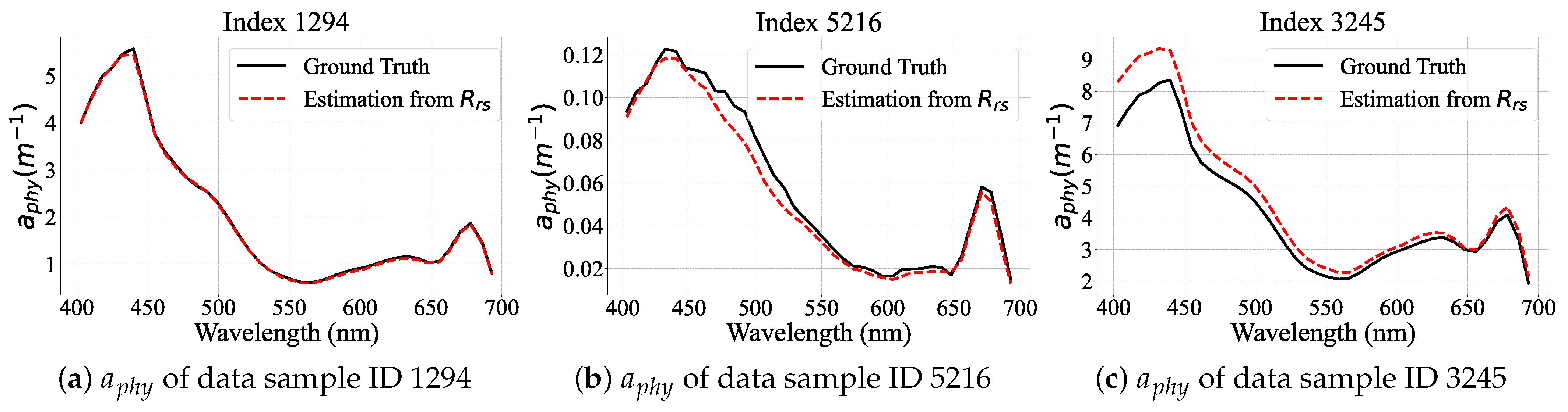
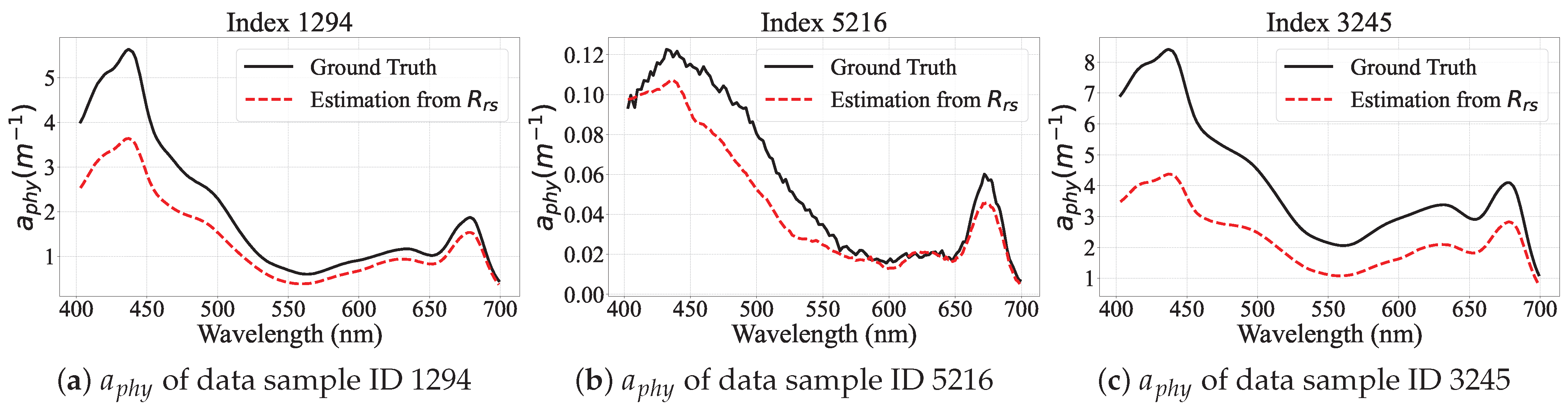
Performance Visualization of PhA-MOE model

In this section, we first present the performance metrics for the PhA-MOE models on each wavelength. The NRMSE ( λ ) , MDSA ( λ ) , SSPB ( λ ) , and Slope ( λ ) values for each wavelength in the EMIT and PACE spectral settings are shown in Figure 3 and Figure 4, respectively.
These metrics allow for a detailed assessment of model performance at different wavelengths for all test samples. From the results, PhA-MOE demonstrates strong performance across all metrics throughout the spectrum. Overall, EMIT data (Figure 3) demonstrated better performance than the PACE data (Figure 4). We attribute this performance difference to the contradiction between the limited data set size and large number of output parameters to learn in the MDN backbone used in the PhA-MOE model. Specifically, the output dimension of MDN grows quadratically with the number of a p h y spectral bands, which are 144 for PACE signals and 40 for EMIT signals. In other words, there are 13 times more parameters to learn when training an MDN for PACE signals compared with EMIT signals.
In particular, for both EMIT and PACE wavelength settings (Figure 3 and Figure 4), PhA-MOE achieves lower NRMSE values in the 400–500 nm range, followed by the 600–700 nm range, compared with the 500–600 nm range. A similar trend is observed across other metrics as well, which suggests that the a p h y values in the range of 500–600 nm, typically lower in magnitude, show poorer performance compared with higher values. This could be attributed to the logistic scaling on a p h y not sufficiently expanding the smaller values into a clearly distinguished value space for effective learning.
Further, we displayed the a p h y estimations at three key wavelengths: near 440 nm and 670 nm for Chl-a absorption and 620 nm for phycocyanin absorption. The results are shown in Figure 5 for the EMIT setting at 440, 618, and 671 nm and in Figure 6 for PACE at 440, 620, and 673 nm. Accurate retrievals of a p h y at these three wavelengths are also highly beneficial for further estimating Chl-a using 670 nm and phycocyanin concentrations using 620 nm. For Figure 5 and Figure 6, we selected the best-performing seed for the PhA-MOE model based on the NRMSE value on the validation set. The PhA-MOE model demonstrates strong agreement between predicted and true values across all wavelengths, with the lowest NRMSE observed at 440 nm (0.53, ε = 23.10%), followed by 671 nm and 618 nm for the EMIT setting. In contrast, the PACE results (Figure 6) exhibit slightly higher NRMSE values at all wavelengths, particularly at 620 nm (NRMSE = 1.21, ε = 31.47%), suggesting reduced model performance on the higher spectral resolution PACE setting. Nonetheless, the fitted regression lines remain close to the 1:1 reference line, and the slopes and scatter are reasonably consistent, indicating that PhA-MOE still generalizes well despite the increased spectral complexity.
To further illustrate the performance of a p h y predictions, it is important not only to focus on improved evaluation metrics but also to examine the spectral shape by overlaying the estimated a p h y onto the field measurements of a p h y across the spectra to assess whether PhA-MOE effectively captures subtle spectral variations rather than merely fitting dominant features of a p h y near Chl-a absorption peaks at 440 and 670 nm. While these dominant features are clearly represented in the scatter plots, more subtle variations, such as those in the range of 450–500 nm influenced by chlorophyll c (Chl-c) and some other photosynthetic carotenoids, are more challenging to capture, which are critical for differentiating phytoplankton groups. Estimated a p h y spectra from testing set data are shown in Figure 7 and Figure 8 for EMIT and PACE spectral settings, respectively, demonstrating good alignment between predicted and actual values. For the EMIT setting, we present the best, 50th-best, and 100th-best fitted curves and then adopt the same target a p h y spectra to the PACE setting for comparison. Note that these selected targets may not correspond to the best, 50th-best, and 100th-best fitted curves in the PACE setting.
In Figure 7, the EMIT results for the best, 50th-best, and 100th-best fitted curves all show excellent alignment between the predicted and actual in the range of 550–680 nm, where chlorophylls a, b, and c have overlapping absorption features. For Figure 7a–c, the a p h y spectra exhibit spectral characteristics typical of cyanobacteria-dominated waters (e.g., Microcystis spp.), with notably high absorption at 440 nm—indicative of bloom conditions. In contrast, Figure 7b, corresponding to Index 5216, displays spectral features more representative of clearer waters, where pico-eukaryotes and cyanobacteria (e.g., prochlorococcus) are likely the dominant phytoplankton group. However, in the 450–500 nm range (Figure 7b), the model shows slight discrepancies between the predicted and actual a p h y values, despite this being among the top 50 best-fitted cases. One possible reason is the overall low magnitude of a p h y in this sample—around 0.12 at 440 nm—meaning that even a moderate absolute error results in a relatively high NRMSE, which can mask poor spectral alignment. This highlights the importance of visually assessing the full spectral shape, not just relying on summary metrics. Additionally, in the 100th-best example shown in Figure 7c, the prediction in the 400–450 nm range deviates more from the ground truth compared with other wavelengths, even though the overall spectral shape remains well aligned. Overall, with EMIT’s 7.4 nm spectral resolution, the predicted a p h y spectra effectively capture signatures of different phytoplankton groups. This demonstrates the potential of using PhA-MOE and EMIT data to derive phytoplankton community composition (PCC), paving the way for applications in future missions such as SBG.
In contrast, the a p h y predictions at the PACE wavelength settings—corresponding to the same sample IDs but not necessarily the best, 50th-best, or 100th-best fits—show that while the spectral shapes are well captured, the magnitudes are consistently underestimated across all three cases, as shown in Figure 8a–c.

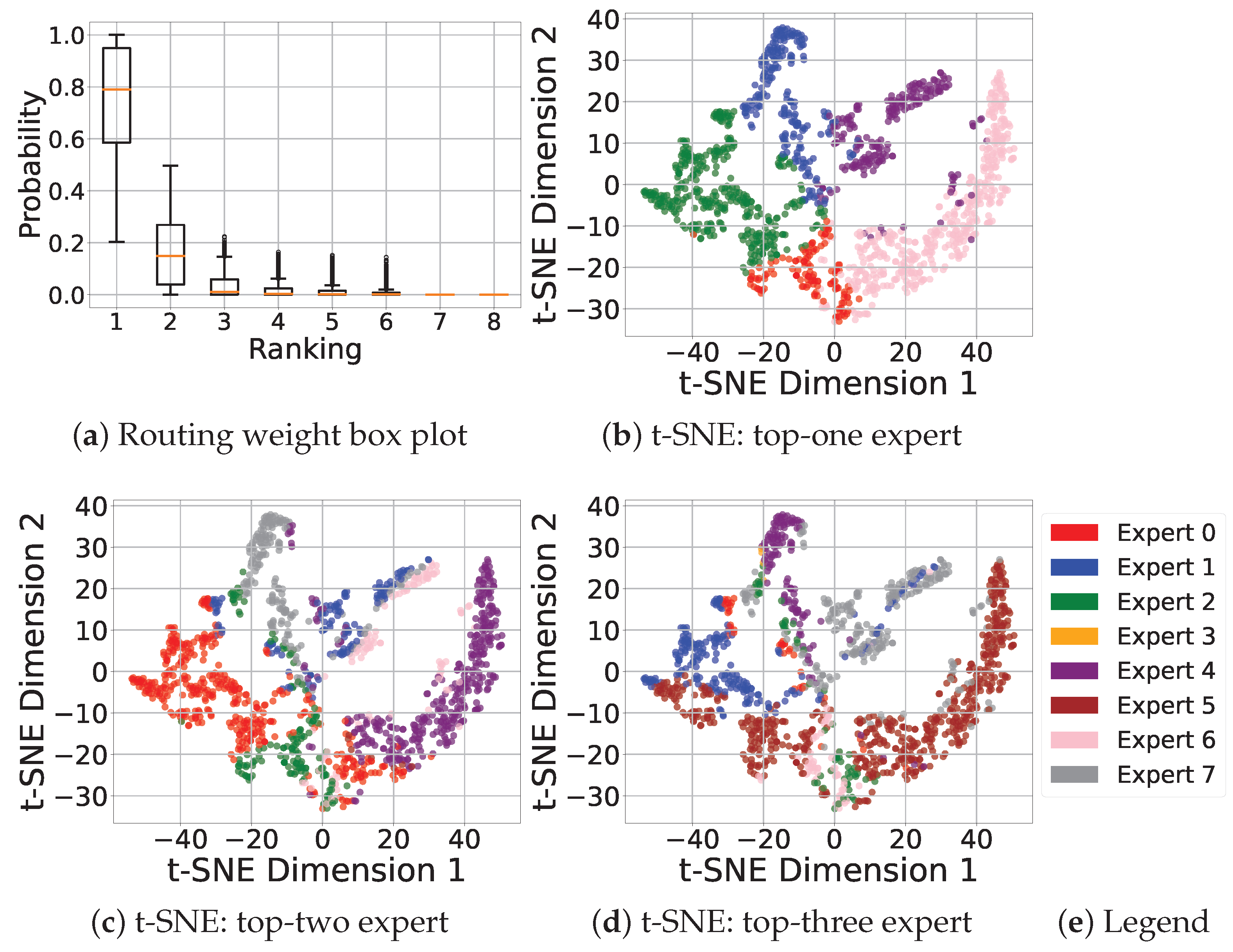
4.4. Visualization of MOE Learning

In this section, we present a visualization of MOE learning to illustrate how the MOE structure assigns data samples to different experts, effectively handling the heterogeneous data pattern. The optimal MOE structure for the EMIT wavelength setting consists of eight experts, with the model activating the six most relevant experts for each input data sample. In other words, the PhA-MOE model utilizes a total of eight experts, with six contributing to the final prediction of each input. Note that these six activated experts have unequal influences on the final estimation, as their individual outputs are weighted and summed based on the routing weights (also known as the gating function values) as introduced in Appendix A.
To visualize the behavior of the gating network, we present the box plot of routing weights for the EMIT wavelength setting in Figure 9a. For each data sample, the routing weights are ranked in descending order, and the distribution of these weights is shown using a box diagram for each expert rank across the entire training set. Since the model activates only the top six experts, the routing weights of the ’top-7’ and ’top-8’ experts are always zero. As shown in Figure 9a, each data sample is primarily processed by its three most relevant experts (’top-1’, ’top-2’, and ’top-3’), demonstrating the specialization of each expert in handling different data distributions.
An efficient MOE structure should be capable of softly partitioning the data space, allowing different experts to handle distinct data clusters. To illustrate this effect, we visualize the training data space using two-dimensional (2D) t-distributed stochastic neighbor embedding (tSNE), as shown in Figure 9b–d, where each data sample is color-coded according to its assigned expert indices. The result in Figure 9b–d reveals a clear clustering pattern in the data space, particularly for the top-one routing weights as shown in Figure 9b–d, where each cluster is predominantly handled by a specific expert. This is consistent with the observation from Figure 9a, which indicates the top-one expert contributes most significantly to the final prediction. The rest of the lower-ranked experts in Figure 9b–d (especially the top two and top three) show different partitioning patterns, with more experts activated and overlapping responsibilities. This results in a more complex division of the data space, indicating collaborations among experts for nuanced predictions, as shown in Figure 9b. These results validate the effectiveness of PhA-MOE in managing data heterogeneity by assigning specialized experts to distinct data distributions, demonstrating its ability to adaptively learn and capture complex spectral patterns.
An efficient MOE also enhances the model’s explainability by aligning each expert’s data space patterns with domain knowledge. For example, in natural language processing tasks, MOE models have been shown to assign different types of words (e.g., nouns, verbs, and adjectives) to different experts for processing [42]. Similarly, we expect the PhA-MOE model used in this study to reflect bio-optical knowledge by assigning experts based on spectral characteristics associated with different water types. To further explore the relationship between expert assignments and bio-optical properties, we labeled each data sample with its corresponding water type following the classification proposed in [43]. This classification, based on GLORIA data, defines three distinct water types. Type I represents clear waters, where phytoplankton presence is minimal, and the spectra are dominated by blue and green reflectance. Type II corresponds to green waters typically associated with phytoplankton blooms—often cyanobacteria—characterized by R r s ( 665 ) > R r s ( 492 ) . Type III includes turbid waters, distinguished by strong red and near-infrared reflectance due to high concentrations of TSS. This labeling allows us to assess whether the PhA-MOE model’s expert assignments align with known spectral characteristics of different water types, thereby enhancing the interpretability of the model, as illustrated in Figure 10a.
To investigate whether the PhA-MOE model captures water-type-specific patterns through its expert assignments, we performed a three-dimensional (3D) tSNE visualization of the gating vectors. Each data point is colored according to its corresponding water type label. As shown in Figure 10b, samples belonging to the same water types (e.g., water types I and II) tend to form distinct clusters in the gating vector space. This clustering indicates that the MOE routing mechanism is sensitive to underlying water-type spectral characteristics. These results demonstrate the interpretability of the MOE structure and its effectiveness in handling heterogeneous data distributions by assigning specialized experts aligned with domain-relevant patterns. Figure 10b also shows that most data points in the GLORIA dataset belong to Water Type I and Type II.

4.5. PhA-MOE Implementation on Field and PACE-OCI Observations

In addition to the training dataset in [10], introduced in Section 2.1.1, additional field data collected from Lake Pontchartrain, Terrebonne Bay, and Barataria Bay in the Gulf estuaries, as described in Section 2.1.2, were further used to evaluate the performance and test the generalizability of the pre-trained and fine-tuned PhA-MOE and MDN frameworks in predicting a p h y . This dataset includes R r s and a p h y measurements from 35 stations, matched with hyperspectral imagery from PACE-OCI acquired on 19 September 2024, 25 September 2024, and 24 October 2024. The model’s performance was further evaluated using matched PACE hyperspectral imagery acquired on the same day as the field observations.

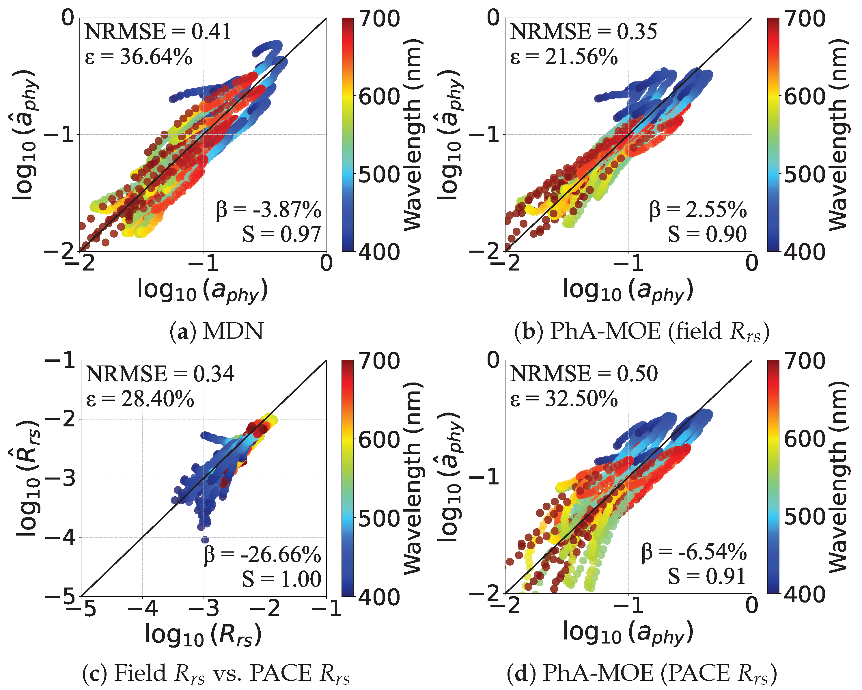
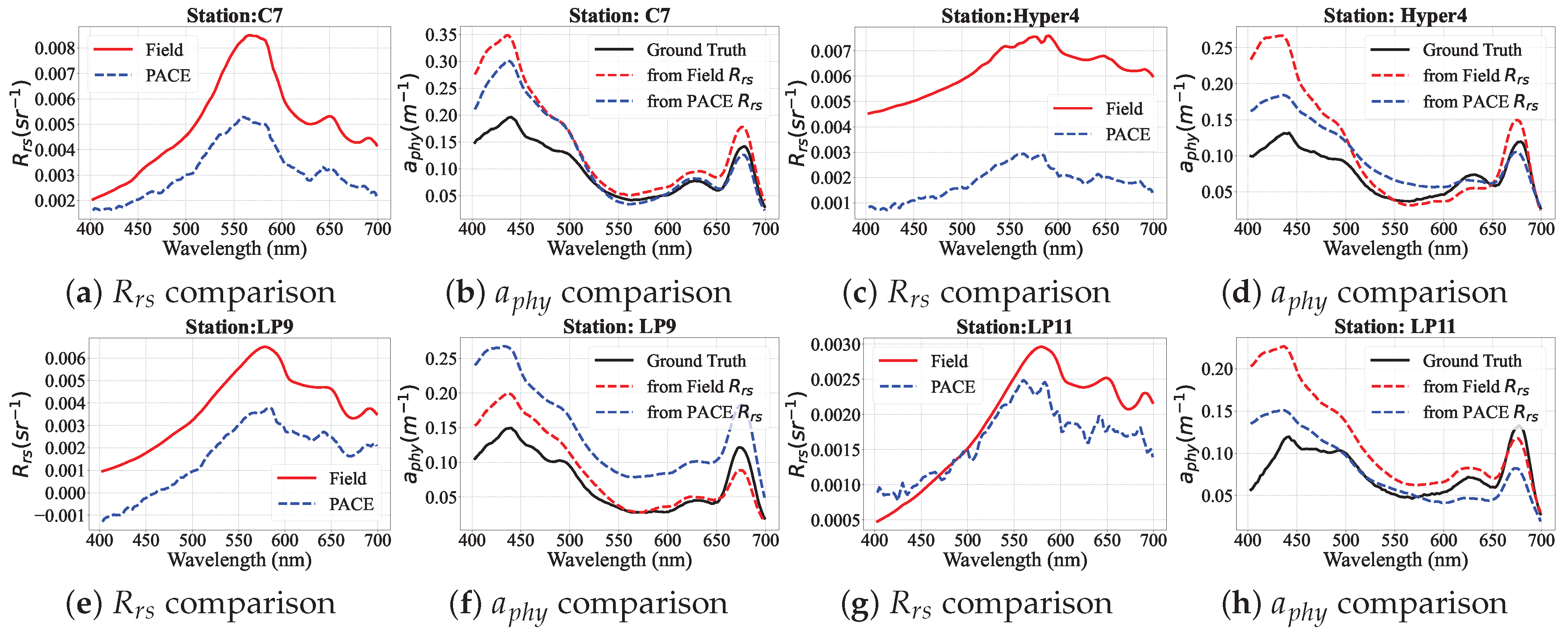
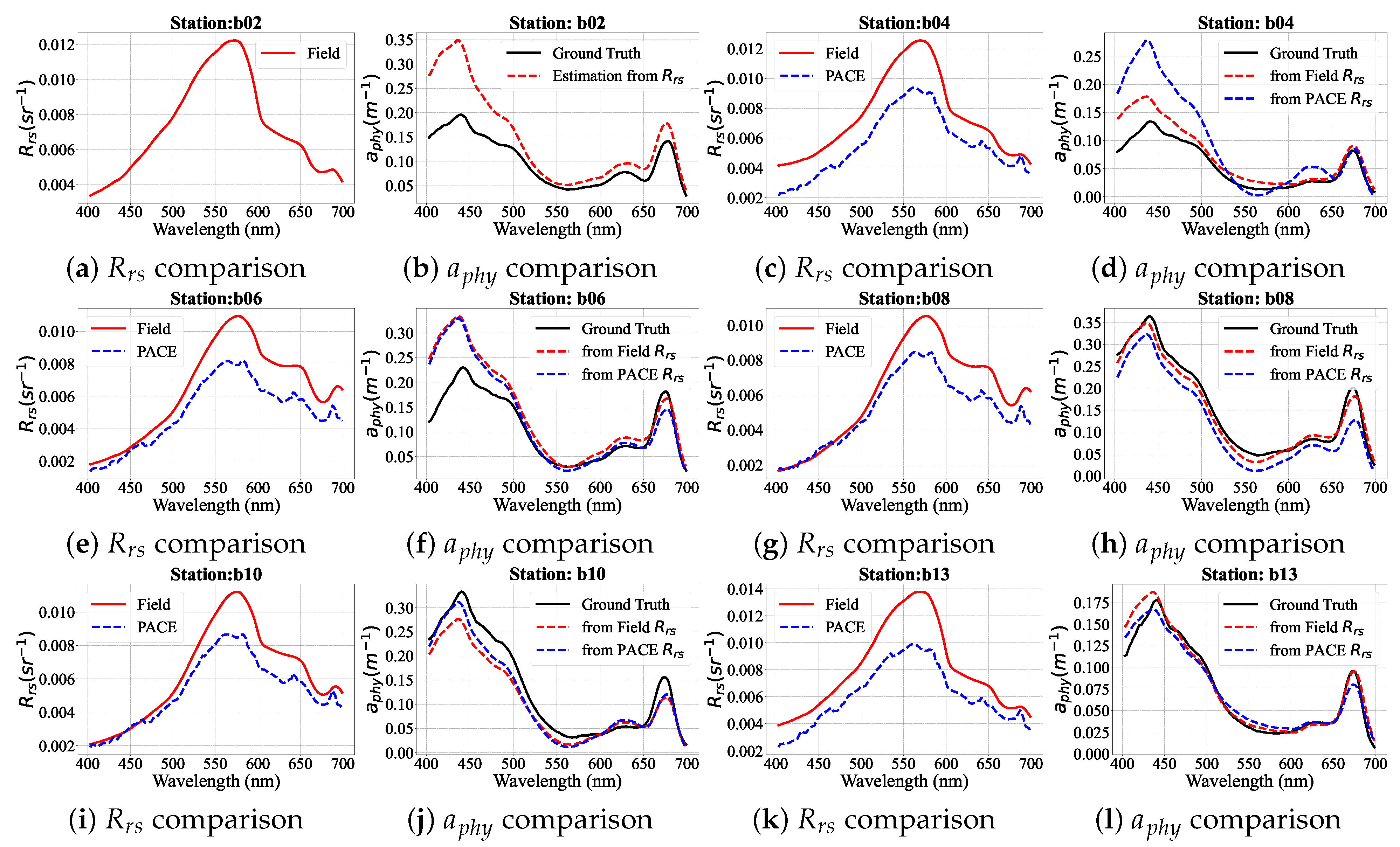
4.5.1. Comparison of Generalizability Between PhA-MOE and MDN
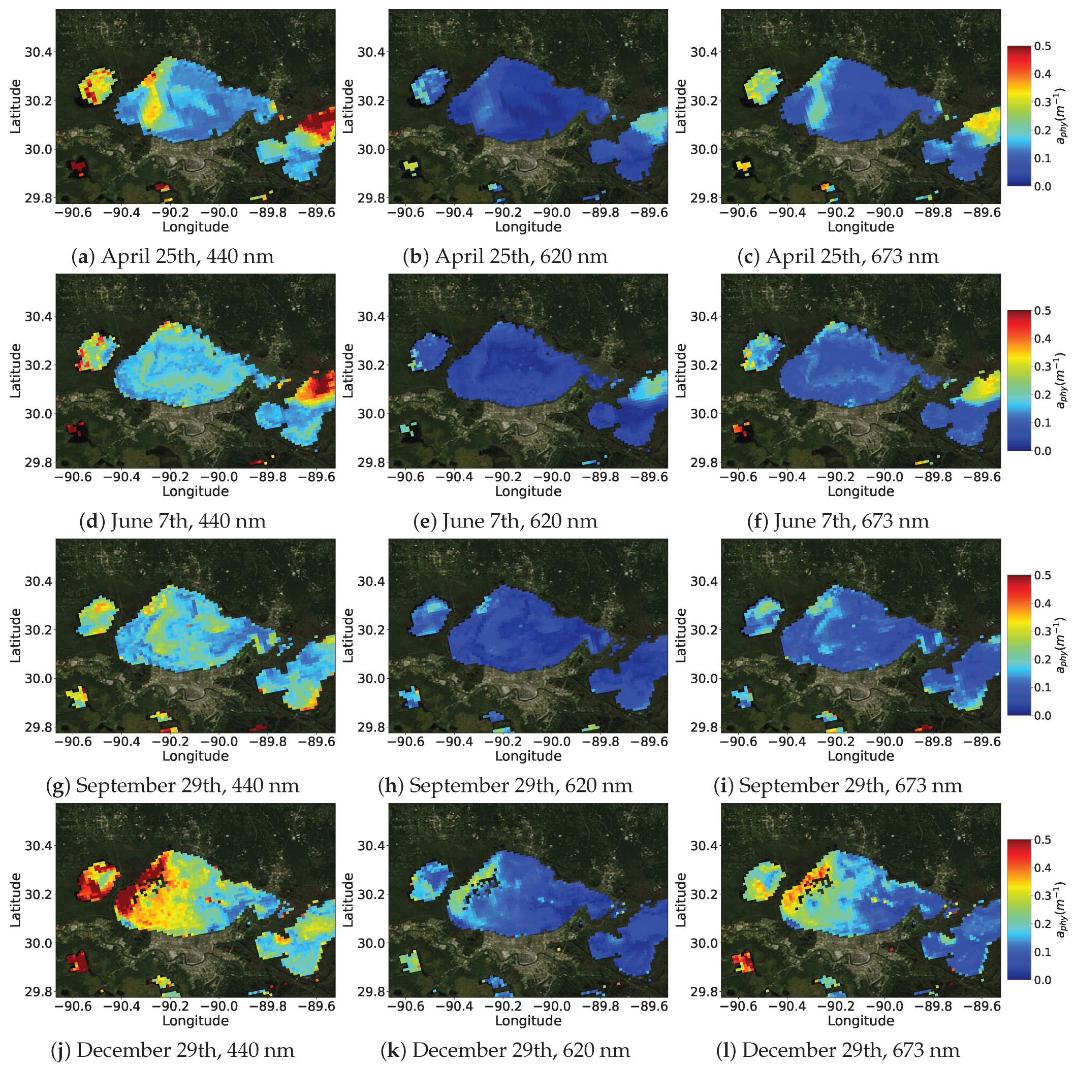
We split the field dataset into two parts: 21 samples were used for additional training, and 14 data samples were used for validation. To construct the new training set, we randomly select 20% of the original training samples and combine them with the 21 field samples. The updated validation set includes the original validation set along with the rest of the 14 field samples. This integration of the field dataset with a subset of the original training dataset helps prevent overfitting during the fine-tuning by maintaining diversity in the training data. Subsequently, this fine-tuning process was performed on the pre-trained PhA-MOE and MDN models. We compared the performance of the fine-tuned PhA-MOE and MDN models using 14 testing field samples at PACE wavelength settings, as well as PACE-derived R r s spectra at the corresponding locations of those 14 sites. The result is shown in Table 5, where PhA-MOE outperforms MDN both before and after fine-tuning the field data. For example, in the best-seed performance after fine-tuning, the NRMSE of PhA-MOE is 0.35, compared with 0.41 for MDN. Similarly, the MDSA value for PhA-MOE is reduced to 21.56, compared with 36.64 for MDN. This experiment shows improved generalizability of the proposed PhA-MOE model over the conventional MDN model, validating the effectiveness of the MOE framework in handling data heterogeneity and improving model generalizability.
We further compare the best-seed performance of the two models after fine-tuning for the a p h y predictions. As visualized in Figure 11a,b, PhA-MOE exhibits a more accurate regression pattern than MDN, with predictions more tightly aligned with the ground truth in the 500–700 nm range and slightly better performance in the 400–500 nm range.

4.5.2. PhA-MOE for a p h y Map Prediction

The fine-tuned PhA-MOE model from Section 4.5.1 was further applied to the corresponding PACE-derived R r s at the same 14 sites. When comparing field-measured R r s with PACE-derived R r s (Figure 11c), we find that they generally agree well, with a slope S = 1 , NRMSE = 0.34 , and a symmetric error of 28.40 % (MDSA, denoted as ϵ ). However, some discrepancies were observed in the blue spectral region, where PACE tends to overcorrect the blue wavelengths, underestimating the R r s values. The predicted a p h y results from PACE R r s compared against field-measured a p h y are presented in Figure 11b,d, revealing a weaker relationship compared with the model’s performance on field data.
To further evaluate the model’s performance on PACE-OCI hyperspectral imagery, we first compared the spectral profiles of field-measured and PACE-derived R r s . As illustrated in Figure 12, Figure 13 and Figure 14, the field-measured R r s spectra (red lines) are generally higher in magnitude than PACE-OCI R r s (blue lines), while PACE effectively captures the overall spectral shape, especially in the spectral range of 500–700 nm. Further, for a p h y predictions, the validation results confirm that the pre-trained PhA-MOE model, with minimal fine-tuning, performs well on both in situ R r s and PACE-OCI R r s in Lake Pontchatrain at the regional level, demonstrating its generalizability as shown in Figure 11b,c. Specifically, when using in situ R r s , the model achieves an NRMSE of 0.36 and a symmetric error (MDSA, denoted as ϵ ) of 23.22% for a p h y prediction, with a strong correlation to in situ a p h y (slope = 0.88). When applied to PACE-derived R r s , the model maintains comparable performance, achieving an NRMSE of 0.50 and Slope = 0.91, although the symmetric error increases to 32.50% and bias rises to 6.54%. The higher errors observed with PACE-derived R r s could be attributed to residual uncertainties in atmospheric correction or the time difference between in situ R r s and PACE R r s . Nonetheless, the strong overall agreement between the two validation sets highlights the robustness of the PhA-MOE model with fine-tuning and its practical applicability to real hyperspectral imagery. This represents the first demonstration of applying an AI model to PACE data with validation, though there is still room for improvement.
Examining individual sites provides a better understanding of the factors contributing to prediction errors in Figure 11b,d. The validation results reveal several key patterns when comparing a p h y predictions from PACE R r s (blue lines) and in situ R r s (red lines) against in situ a p h y (black lines) in Figure 12, Figure 13 and Figure 14. At sites such as LP9, T14, and TC7, where PACE-OCI R r s is consistently lower than in situ R r s , we observe an overestimation of a p h y from PACE R r s . This suggests that discrepancies in R r s magnitude are one of the most direct factors affecting the accuracy of a p h y retrieval, leading to systematic biases in the estimates. Furthermore, some field-measured spectra exhibit atypical characteristics—for example, cases where a p h y at 440 nm is lower than at 670 nm, indicating stronger absorption in the red region compared with the blue. This is not typical of standard a p h y spectra and is likely due to the pigment packaging effect [44], such as observed at Hyper 4 and LP11 (Figure 12d,h) or b06 (Figure 14f), which show broad absorption features between 440 and 500 nm. The pigment packaging effect causes the absorption spectra to flatten, especially at peak absorption wavelengths (e.g., 440 nm for Chl-a). In these cases, the model struggles to accurately predict both the magnitude and spectral shape of a p h y . This limitation is understandable, as spectra of this type are extremely underrepresented in the training dataset. However, this type of a p h y spectra has also been frequently observed in lakes ([45]), where the blue-to-red absorption ratio of phytoplankton tends to decrease in lakes with higher CDOM content. Consequently, spectral mismatches or uncertainties in the model’s ability to resolve this specific type of absorption feature, particularly when the spectral slope deviates from typical Chl-a absorption patterns, may contribute to the observed discrepancies. Lastly, in Figure 14, the overall performance of PhA-MOE in predicting a p h y for both PACE R r s and in situ R r s appears to be more reliable compared with Figure 12 and Figure 13. This improvement is likely due to better alignment between in situ and PACE R r s , as well as a shorter time gap between the two observations. Moreover, it highlights the critical role that R r s quality plays in accurately predicting a p h y using the PhA-MOE model.
After validating the PhA-MOE model using field a p h y data (Figure 11b,d, Figure 12, Figure 13 and Figure 14), we applied the model directly to PACE-OCI R r s imagery (version 2) to generate a p h y maps for Lake Pontchartrain, enabling an assessment of its spatial and temporal variability. This marks the first application of PACE-OCI hyperspectral imagery in optically complex waters in estuaries to study a p h y across seasons since PACE’s launch on 8 February 2024.
Figure 15 presents the match-up PACE-OCI imagery acquired on 23 September 2024 alongside in situ observations in Figure 12. The RGB image (Figure 15a) captures the overall water conditions, with variations in color likely indicating differences in CDOM, TSS, and phytoplankton abundance and community composition. The a p h y at 440 nm (Figure 15b) shows absorption values ranging from 0 to 0.5, indicating moderate phytoplankton biomass in certain regions. Meanwhile, the low absorption at 620 nm (Figure 15c) indicates minimal phycocyanin presence, suggesting that cyanobacteria were not dominant during this period. In addition, a p h y at 670 nm (Figure 15d) shows lower values compared with a p h y at 440 nm, which is consistent with typical a p h y spectral characteristics.
Figure 16 presents PACE-derived a p h y at three wavelengths (440 nm, 620 nm, and 673 nm) for four different dates: 25 April, 7 June, 29 September, and 29 December 2024 to examine seasonal and spatial variations in phytoplankton absorption, with particular focus on chlorophyll-a and phycocyanin dynamics. From the results, seasonal variations in a p h y are evident, with noticeable differences in absorption intensity across different months. For instance, certain regions, such as in the northwestern–central part of Lake Pontchartrain, exhibit higher absorption at 440 nm and 673 nm, while 620 nm absorption remains low in most cases. However, on 29 December 2024, localized increases in 620 nm absorption are observed near the area connected to the Tangipahoa River, suggesting cyanobacterial activity in those areas. Additionally, a high discharge from the Amite River was observed in December, flowing into Lake Maurepas, which is connected to Lake Pontchartrain through Pass Manchac, likely also contributing to the cyanobacteria bloom. In addition, on 7 June 2024, cyanobacteria signals were also detected in Lake Borgne. These examples demonstrate the ability of PACE hyperspectral imagery to capture seasonal and spatial dynamics of phytoplankton communities, offering valuable insights into Chl-a and phycocyanin variability in estuarine environments. These results reveal a clear change in the spatial distribution of a p h y that is significantly higher in December compared with April, June, and September, with the lowest levels observed in April due to the discharges of tributaries in the northern shore of the lake leading to nutrient-rich waters in December. This study demonstrates the capability of PACE data to detect phytoplankton dynamics in estuarine waters and emphasizes the potential for using hyperspectral remote sensing to monitor seasonal and spatial variations in phytoplankton communities.

5. Discussion

5.1. Data Preprocessing

Our experimental results highlight the importance of data preprocessing in training effective neural networks for a p h y prediction. This is primarily due to the heavy-tailed distribution of both input and output data, where the large outliers significantly exceed the 75 % quartile value. In this study, we tested two different preprocessing strategies: (1) WB—applying the same scale to the entire spectral signal, preserving the spectral shape of bio-optical signals, and (2) WL—applying different scalers to different wavelengths of the signal. Intuitively, the former WB approach is preferred as it preserves the spectral shape, while the WL approach ensures the data remains within a more reasonable value range.
For the PACE wavelength setting, applying a uniform scaler to the entire signal yields the best results. Interestingly, the experimental results show that the EMIT dataset benefits more from the WL approach. This suggests that the neural network is still able to extract the necessary features for a p h y estimation, processing signals in a more abstract and flexible manner. This phenomenon could be attributed to the relatively lower resolutions of EMIT (7.4 nm) compared with PACE (2.5 nm), where high-resolution spectral information in PACE carries important interband relationships that could be distorted by WL preprocessing. Given these findings, the WL method may also be well-suited for a p h y prediction using multispectral sensors such as Sentinel-2 MSI or Sentinel-3 OLCI, whereas the WB approach appears more appropriate for high-spectral resolution datasets.
These findings suggest that neural networks are capable of extracting valuable bio-optical information even when preprocessing alters the spectral shape of the signal. This opens the door to further exploration of hybrid preprocessing strategies that combine the strengths of both approaches—preserving spectral shape while enhancing data normalization. Such combinations may improve performance across a wider range of datasets and contribute to more robust and generalizable machine-learning models for a p h y prediction.

5.2. Model Implementation of Satellite Imagery

When the PhA-MOE model trained on field observations is applied to satellite imagery, several factors contribute to its reduced performance. One of the most critical factors is the quality of satellite-derived R r s , as the water-leaving signal typically accounts for only about 10% of the top-of-atmosphere radiance [46]. Atmospheric correction in coastal areas is particularly challenging due to the complex aerosol composition. This presents a major concern when applying the PhA-MOE framework to PACE-derived R r s , as differences in spectral shape and magnitude were observed and can significantly affect model performance. Based on our field observations (Figure 12, Figure 13 and Figure 14), PACE-derived R r s values are generally lower than in situ measurements under most conditions, although good agreement is observed in some cases. Additionally, PACE R r s spectra tend to be slightly noisier compared with in situ measurements. Furthermore, this discrepancy may also result from differences in spatial resolution. PACE has a spatial resolution of 1.2 km, whereas estuarine environments are highly biogeochemically dynamic. In situ, R r s is collected at a single point, and comparing it to a 1.2 km × 1.2 km satellite pixel inevitably introduces spatial mismatch. This is an unavoidable limitation when using PACE in estuarine–coastal settings. In addition, estuaries also often have high concentrations of CDOM and NAP, which further complicate the signal, especially in the blue–green spectral regions [47]. Additionally, it is difficult to perfectly match the timing of field measurements with satellite overpasses. In most cases, there is a time difference of 2–3 h, which can further contribute to discrepancies between observed and predicted a p h y values. Overall, our field R r s measurements suggest that PACE-OCI performs reasonably well in capturing the spectral shape, but some discrepancies remain in magnitude, particularly at sites with high CDOM and NAP concentrations.

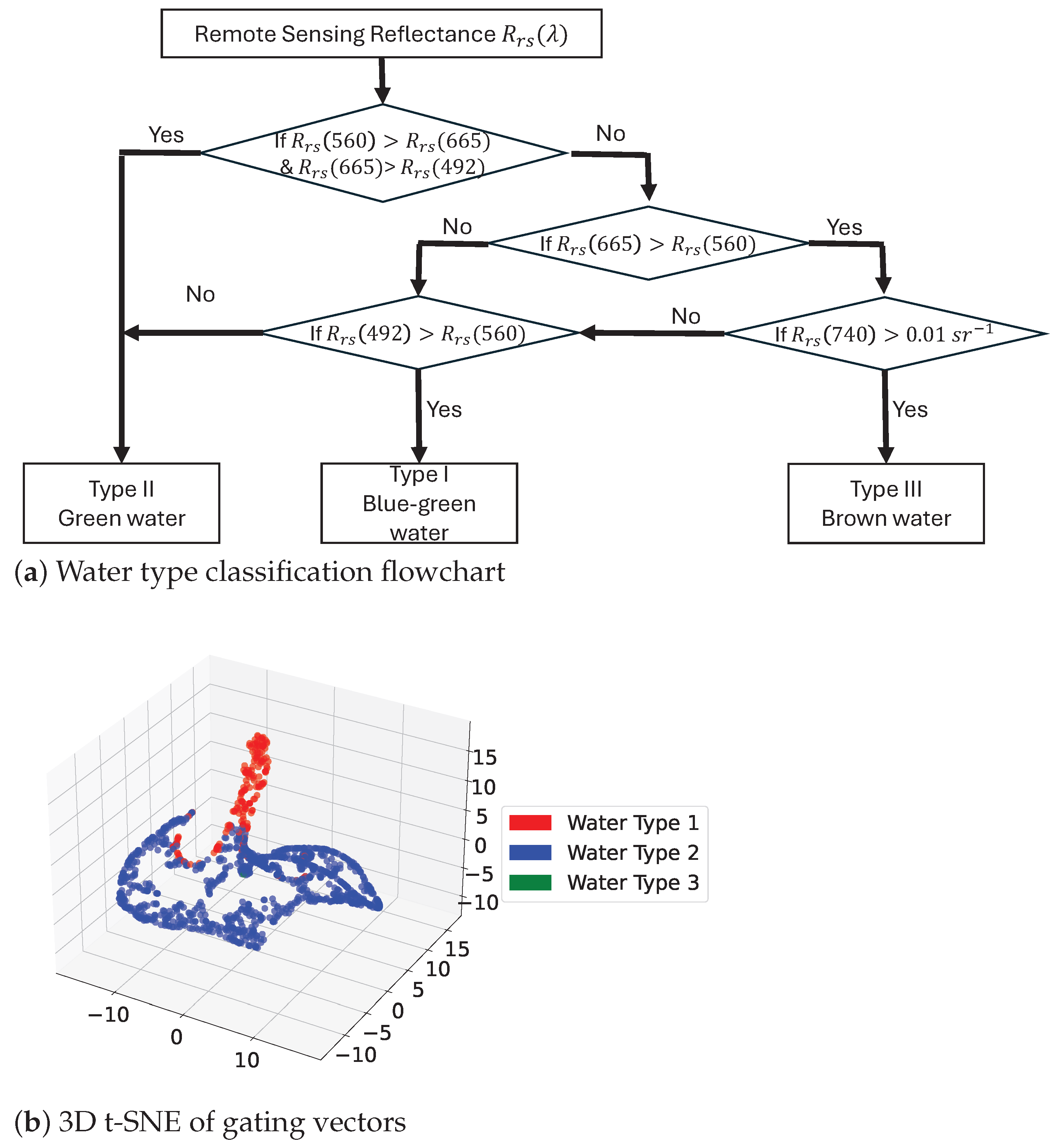
5.3. Interpretability of MOE Structure

The proposed PhA-MOE model consistently outperforms its MDN backbone across evaluation metrics (NRMSE, MDSA, SSPB, and Slope), regardless of whether the entire signal is scaled together or each wavelength is scaled separately. This demonstrates the effectiveness of the MOE structure in handling the heterogeneous data distributions, making it particularly valuable in the ocean color field, where diverse bio-optical properties interact in complex ways to influence R r s . The PhA-MOE framework offers two key advantages: (1) it demonstrates strong performance on the GLORIA dataset by effectively addressing data heterogeneity, and (2) when applied to a new dataset (Lake Pontchartrain), it consistently outperforms the conventional MDN baseline both before and after fine-tuning, indicating promising generalizability.
The MOE structure softly splits the data space into different clusters, with each assigned to specialized sub-networks (experts) for processing. This architecture enhances both model interpretability and alignment with bio-optical properties of waters. Unlike traditional black-box neural networks, MOE-based models offer a structured approach to learning, where different experts focus on distinct spectral characteristics, making the predictions more transparent and physically meaningful. This approach is particularly useful in ocean color remote sensing, where variations in water types, driven by diverse phytoplankton assemblages, as well as differing levels of carbon and sediment concentrations, introduce complexities that traditional models struggle to capture. By leveraging a MOE-based framework, we can develop models that adaptively learn from these variations, leading to more reliable a p h y estimates.
Beyond indicating that MOE can cluster heterogeneous data distributions, the expert top-k routing process enables the model to generalize beyond predefined water type categories. To evaluate the generalizability of the PhA-MOE model on unseen data, we examine the position of data samples in the embedding space as illustrated in Figure 9b, where clusters in different colors represent distinct data patterns. If the new sample falls within one existing cluster, it likely belongs to a data pattern the model has already learned. If it falls in proximity to established clusters, the model can be generalized by combining existing learned patterns. However, if the sample is located far from all clusters, the existing model may not be capable of processing it effectively, where fine-tuning is needed for performance improvement.
Future research should explore incorporating domain knowledge into the initialization of experts, enabling them to specialize in distinct bio-optical conditions, such as coastal vs. open-ocean waters or specific phytoplankton functional types, if more field observations become available in the future. This approach could further enhance the generalizability and accuracy of MOE-based models in global ocean color applications.

5.4. Potentials to Large Phytoplankton Foundation Models

The proposed PhA-MOE model demonstrates strong generalizability when applied to both in situ and PACE-derived R r s , highlighting its practicality for predicting phytoplankton absorption characteristics using hyperspectral satellite data. The results suggest that a pre-trained PhA-MOE model, with minimal fine-tuning, can effectively generalize across different sources of R r s , such as in situ and satellite-derived observations in the Gulf estuaries. This adaptability underscores the potential of MOE-based architectures for developing phytoplankton foundation models similar to large language models. Just as language models are pre-trained on extensive text corpora and fine-tuned for specific tasks, the PhA-MOE model could serve as a base model for phytoplankton absorption retrieval, refining predictions for different aquatic environments with minimal additional training. The strategy of pre-training neural networks on large datasets and fine-tuning with local data offers a scalable and transferable approach, further enhancing the applicability of MOE structures in ocean color remote sensing, such as PACE tested in this study. However, for EMIT, we have not yet obtained paired field observations to match with EMIT imagery. This highlights the need for future efforts to focus on field measurements of bio-optical properties, ensuring that this approach can be properly validated and applied to a broader range of hyperspectral missions.

6. Conclusions

In this work, we introduce PhA-MOE, a novel learning-based framework for hyperspectral retrieval of a p h y powered by MOE. To achieve improved performance in a p h y prediction, we first explored various data preprocessing methods for R r s a p h y spectral data feature extraction and normalization. With the optimal preprocessing methods identified, the innovative MOE structure and a specialized training scheme are applied to MDN for a p h y prediction under EMIT and PACE spectral settings, where PhA-MOE outperforms other SOTA models with the lowest NRMSE, highlighting its improvement in prediction accuracy. Additionally, PhA-MOE demonstrates better symmetric prediction metrics, such as MDSA and SSPB, showing a good balance between the overestimation and underestimation errors. Furthermore, this study presents the first application of the PhA-MOE machine learning model to the newly launched PACE-OCI and EMIT hyperspectral imagery in optically complex estuarine environments. The results from Lake Pontchartrain demonstrate the power of the MOE framework in handling heterogeneous data and highlight its effectiveness in predicting a p h y using hyperspectral imagery. The a p h y maps derived from PhA-MOE in Lake Pontchartrain demonstrate the potential of using hyperspectral imagery to provide detailed insights into the phytoplankton community structure. Promising future directions include exploring the customized MOE architectures integrated with advanced learning models for a p h y prediction, as well as incorporating decoupling modules for the joint retrieval of other optical properties. Another key direction involves integrating physics-inspired feedback mechanisms to leverage domain knowledge more effectively, along with enhanced spatial-spectral feature extraction techniques to improve spatial consistency in ocean color remote sensing analysis.

Author Contributions

Conceptualization, S.Z. and B.L.; methodology, W.W. and S.Z.; software, W.W. and S.G.; validation, W.W., S.G., Y.Z. and J.L.; formal analysis, W.W. and B.L.; investigation, W.W., J.L. and B.L.; resources, J.L. and B.L.; data curation, W.W., J.L. and B.L.; writing—original draft preparation, W.W.; writing—review and editing, W.W., S.Z., B.L. and Z.D.; visualization, W.W. and B.L.; supervision, S.Z., B.L. and Z.D.; project administration, S.Z. and B.L.; funding acquisition, S.Z. and B.L. All authors have read and agreed to the published version of the manuscript.

Funding

This work was supported in part by the National Science Foundation under Grant Nos. 2425811 and 2332760, in part by the National Aeronautics and Space Administration (NASA) PACE program through Grant Nos. 80NSSC24K1415 and 80NSSC24K0865, and in part by the USACE ERDC Freshwater HAB funding support through Grant No. W912HZ-24-2-0016.

Data Availability Statement

PACE-OCI and EMIT data can be accessed from NASA Earthdata Search (https://search.earthdata.nasa.gov/search (accessed on 27 January 2024)). The other data presented in this study are available upon request from the second author. The source code used in this study is publicly available on GitHub. The models were implemented using PyTorch (v2.2.0, CUDA 11.8). This repository provides all the scripts necessary to reproduce the experiments and analyses presented in this manuscript. You can access the repository at https://github.com/wwwangUCD/PhA-MOE (accessed on 11 June 2025). We encourage the community to explore, utilize, and contribute to the codebase to further advance research in this area.

Acknowledgments

The authors gratefully acknowledge Nima Pahlevan and Ryan O’Shea for sharing the R r s a p h y dataset and the NASA PACE program for providing access to the PACE-OCI AOP data.

Conflicts of Interest

The authors declare no conflicts of interest.

Abbreviations

The following abbreviations are used in this manuscript:
IOPsInherent Optical Properties
a p h y Phytoplankton Absorption Coefficient
PPCPhytoplankton Community Composition
MOEMixture of Experts
OCIOcean Color Instrument
PACEPlankton, Aerosol, Cloud, Ocean Ecosystem
EMITEarth Surface Mineral Dust Source Investigation
SBGSurface Biology Geology
HABHarmful Algal Bloom
R r s Remote Sensing Reflectance
IOPInherent Optical Properties
QAAQuasi Analytical Algorithm
GIOPGeneralized IOP Inversion
CDOMColored Dissolved Organic Matter
NAPNon-Algal Particles
AIArtificial Intelligence
ChlaChlorophyll-a
MDNMixture Density Network
TSSTotal Suspended Solids
PCPhycocyanin
MLPMulti-Layer Perceptron
QFTQuantitative Filter Pad Technique
AOPApparent Optical Property
SOTAState-of-the-Art
VAEVariational Autoencoder
2DTwo-Dimensional
3DThree-Dimensional

Appendix A. Technical Details of PhA-MOE

In PhA-MOE, the MOE-based embedding uses a noisy top-k gating network and multiple expert networks [42], implemented using multilayer perceptron (MLPs) [48]. Unlike traditional single-expert-activation neural networks, the MOE gating network dynamically selects the top k most relevant experts for each input, while each expert network specializes in capturing specific patterns within the data distribution. Each expert generates a latent embedding, which is forwarded into the final predictor designed based on MDN framework. This MDN-based predictor follows a structure used in [10], learning a mixture Gaussian probability distribution to characterize the in situ data samples.
The “Top-k weighted sum” block in the embedding module aggregates features from the selected experts as illustrated in Figure 2. The predictor module’s “combination function” process refers to the sampling process from a trained MDN model, which ultimately yields a p h y estimation by drawing from the mixture Gaussian probability distribution corresponding to the input R r s . The loss functions for PhA-MOE consist of the MOE loss [42] and the MDN loss, each with distinct physical interpretations and value ranges [10]. The MOE loss is designed to prevent any single expert from dominating the output or receiving a disproportionate number of samples. In contrast, the MDN loss aims to maximize the likelihood of accurately estimating a p h y . The PhA-MOE model applies these two losses sequentially, ensuring that it effectively balances the experts while also effectively learning the target output distribution.
  • MOE-based Embedding:
As shown in Figure 2, the preprocessed reflectance ( R ˜ r s ) is passed through the gating network in the proposed PhA-MOE, which determines the relevance of each expert for the given input. This process, known as routing, assigns different samples to specific experts, which then process the input independently. The top-k outputs are combined into a weighted sum based on these routing weights.
The output of gating network G ( x ) and i-th expert network E i ( x ) for an input x (specifically R ˜ r s ) is combined as
Y = i = 1 M G ( x ) i · E i ( x ) ,
where M is the number of experts, and G ( x ) i is the weight of the ith expert. To handle over-fitting and encourage diversity, a noisy top-k gating scheme adds sparsity and noise to the classic softmax gating. The weight G ( x ) takes the form of
G ( x ) i = e T k ( H ( x ) ) i j e T k ( H ( x ) ) j ,
where H ( x ) i = ( x · W g ) i + ϵ · log 1 + e ( x · W n ) i , and T k ( v ) i = v i if v i is among the top-k selection; otherwise, T k ( v ) i = .
Here, ϵ is a standard normal random variable and W n is introduced to balance the load of each expert. Meanwhile, H ( x ) i and T k ( v ) i denote the i-th elements of H ( x ) and T k ( v ) , respectively. The combination of embeddings from each selected expert forms latent Y , which is then passed to an MDN-based predictor for final prediction.
  • MDN-based Predictor:
The MDN learns a probability density, formulated as the weighted sum of c Gaussian distributions, expressed as:
p ( a ˜ ^ p h y Y ) = i = 1 c α i ( Y ) ψ i ( a ˜ ^ p h y Y ) ,
where a ˜ ^ p h y is the estimation of the preprocessed a ˜ p h y , ψ i ( a ˜ ^ p h y Y ) represents a multivariate Gaussian with mean μ i and covariance Cov i , and α i ( Y ) are the non-negative mixing coefficients satisfying i = 1 c α i ( Y ) = 1 .
After training, the MDN estimates the conditional probability of a ˜ ^ p h y given input embedding Y . The final estimation of a ˜ p h y is taken as the mean μ i ( Y ) of the Gaussian component with the largest mixing coefficients α i ( Y ) , i.e.,
a ˜ ^ p h y = μ i ( Y ) , where i = arg max α i ( Y ) ,
which refers to the “Combination Function” block in Figure 2. Note that the a ˜ ^ p h y is in the scaled value range, and to get the a p h y estimation in the actual value range (deonted as a ^ p h y ), we use the inverse transform of a p h y scaling.
  • Loss Function:
The loss function for training the PhA-MOE, is defined as
L = L MDN + γ L MOE .
Specifically, we use the same MOE loss as defined in [42]:
L MOE ( X ) = L importance ( X ) + L load ( X ) ,
where X represents a batch of inputs, and x X represents an individual input from the batch. The importance-balancing loss ensures all experts contribute equally to processing inputs, preventing any experts from dominating the training process, and is defined by
L importance ( X ) = w importance · CV ( Importance ( X ) ) 2 ,
where Importance ( X ) = x X G ( x ) , and CV ( · ) represents for the coefficient of variation:
CV ( A ) = std ( A ) E ( A ) ,
where std ( A ) and E ( A ) denote the standard deviation and expected value of A, respectively. A lower value of CV ( Importance ( X ) ) 2 indicates a more uniform distribution of importance across experts. The load-balancing loss is defined as:
L load ( X ) = w load · CV ( Load ( X ) ) 2 ,
where Load ( X ) i = x X P ( x , i ) , and P ( x , i ) represents the probability that expert i processes input x . This loss addresses the imbalance in the number of examples assigned to each expert.
For the MDN loss, we utilize the likelihood function for the joint probability, defined as:
L MDN = ln i = 1 c α i ( Y ) ψ i ( a p h y Y ) .
Both L MOE and L MDN are essential, but operate on different scales. To address this, our method trains the model using these two losses sequentially. Specifically, for each batch of training data, we alternate between optimizing L MOE and L MDN . This strategy ensures that the model effectively balances the contributions of the experts while simultaneously learning the correct output distribution.

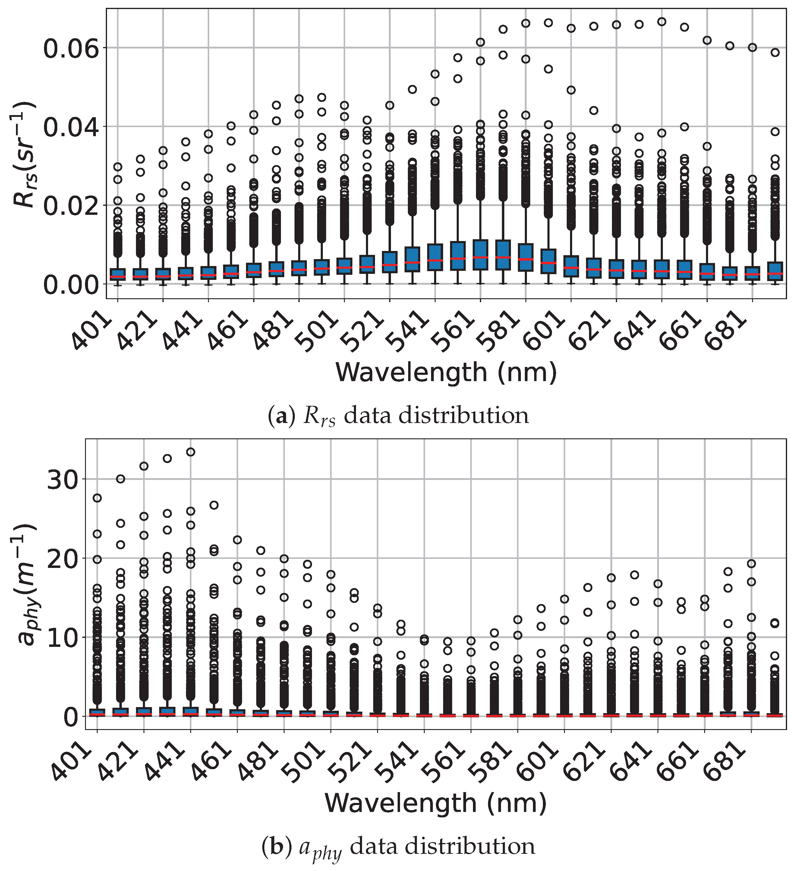
Appendix B. Box Plot Visualizations of Preprocessed Rrs and aphy

Figure A1. Boxplot visualization of R r s and a p h y on each wavelength after preprocessing. (a,b) WL and WB preprocessing on R r s , respectively. (c,d) WL and WB preprocessing on a p h y , respectively.
Remotesensing 17 02103 g0a1

Appendix C. Stability Analysis Across Random Seeds

Table A1 presents the performance of each method over different random seeds in terms of the coefficient of variation as defined in Equation (A6). Compared with other models, the proposed PhA-MOE model shows a smaller performance variation in various experimental setups and random seeds, indicating its superior robustness and stability.
Table A1. Coefficient of Variation (CV) of performance metrics across random seeds.
ResolutionModel CV ( NRMSE ) CV ( ϵ ) CV ( | β | ) CV ( | S 1 | )
EMITMDN0.34870.10090.51630.6850
PhA-MOE0.23590.07230.52260.5054
MLP0.40530.12700.41340.1924
VAE0.23950.14880.73820.3965
PACEMDN0.14640.12060.43860.4120
PhA-MOE0.09580.08430.20920.2631
MLP0.32880.12450.45510.1956
VAE0.43230.15550.64260.4813

References

  1. Henson, S.A.; Cael, B.; Allen, S.R.; Dutkiewicz, S. Future phytoplankton diversity in a changing climate. Nat. Commun. 2021, 12, 5372. [Google Scholar] [CrossRef] [PubMed]
  2. Liu, B.; D’Sa, E.J.; Maiti, K.; Rivera-Monroy, V.H.; Xue, Z. Biogeographical trends in phytoplankton community size structure using adaptive sentinel 3-OLCI chlorophyll a and spectral empirical orthogonal functions in the estuarine-shelf waters of the northern Gulf of Mexico. Remote Sens. Environ. 2021, 252, 112154. [Google Scholar] [CrossRef]
  3. Xi, H.; Hieronymi, M.; Röttgers, R.; Krasemann, H.; Qiu, Z. Hyperspectral Differentiation of Phytoplankton Taxonomic Groups: A Comparison between Using Remote Sensing Reflectance and Absorption Spectra. Remote Sens. 2015, 7, 14781–14805. [Google Scholar] [CrossRef]
  4. Liu, B.; D’Sa, E.J.; Joshi, I.D. Floodwater impact on Galveston Bay phytoplankton taxonomy, pigment composition and photo-physiological state following Hurricane Harvey from field and ocean color (Sentinel-3A OLCI) observations. Biogeosciences 2019, 16, 1975–2001. [Google Scholar] [CrossRef]
  5. Dierssen, H.M.; Ackleson, S.G.; Joyce, K.E.; Hestir, E.L.; Castagna, A.; Lavender, S.; McManus, M.A. Living up to the hype of hyperspectral aquatic remote sensing: Science, resources and outlook. Front. Environ. Sci. 2021, 9, 649528. [Google Scholar] [CrossRef]
  6. Lee, Z.; Carder, K.L.; Arnone, R.A. Deriving inherent optical properties from water color: A multiband quasi-analytical algorithm for optically deep waters. Appl. Opt. 2002, 41, 5755–5772. [Google Scholar] [CrossRef]
  7. Roesler, C.S.; Boss, E. Spectral beam attenuation coefficient retrieved from ocean color inversion. Geophys. Res. Lett. 2003, 30. [Google Scholar] [CrossRef]
  8. Werdell, P.J.; Franz, B.A.; Bailey, S.W.; Feldman, G.C.; Boss, E.; Brando, V.E.; Dowell, M.; Hirata, T.; Lavender, S.J.; Lee, Z.; et al. Generalized ocean color inversion model for retrieving marine inherent optical properties. Appl. Opt. 2013, 52, 2019–2037. [Google Scholar] [CrossRef]
  9. Zhu, Q.; Shen, F.; Shang, P.; Pan, Y.; Li, M. Hyperspectral remote sensing of phytoplankton species composition based on transfer learning. Remote Sens. 2019, 11, 2001. [Google Scholar] [CrossRef]
  10. Pahlevan, N.; Smith, B.; Binding, C.; Gurlin, D.; Li, L.; Bresciani, M.; Giardino, C. Hyperspectral retrievals of phytoplankton absorption and chlorophyll-a in inland and nearshore coastal waters. Remote Sens. Environ. 2021, 253, 112200. [Google Scholar] [CrossRef]
  11. Mobley, C.D. Light and Water: Radiative Transfer in Natural Waters; Academic Press: San Diego, CA, USA, 1994. [Google Scholar]
  12. Gordon, H.R.; Brown, O.B.; Evans, R.H.; Brown, J.W.; Smith, R.C.; Baker, K.S.; Clark, D.K. A semianalytic radiance model of ocean color. J. Geophys. Res. Atmos. 1988, 93, 10909–10924. [Google Scholar] [CrossRef]
  13. Roesler, C.; Pery, M. In situ phytoplankton absorption, fluorescence emission, and particulate backscattering spectra determined from reflectance. J. Geophys. Res. 1995, 100. [Google Scholar] [CrossRef]
  14. Pahlevan, N.; Smith, B.; Schalles, J.; Binding, C.; Cao, Z.; Ma, R.; Alikas, K.; Kangro, K.; Gurlin, D.; Hà, N.; et al. Seamless retrievals of chlorophyll-a from Sentinel-2 (MSI) and Sentinel-3 (OLCI) in inland and coastal waters: A machine-learning approach. Remote Sens. Environ. 2020, 240, 111604. [Google Scholar] [CrossRef]
  15. O’Shea, R.E.; Pahlevan, N.; Smith, B.; Boss, E.; Gurlin, D.; Alikas, K.; Kangro, K.; Kudela, R.M.; Vaičiūtė, D. A hyperspectral inversion framework for estimating absorbing inherent optical properties and biogeochemical parameters in inland and coastal waters. Remote Sens. Environ. 2023, 295, 113706. [Google Scholar] [CrossRef]
  16. Lehmann, M.K.; Gurlin, D.; Pahlevan, N.; Alikas, K.; Conroy, T.; Anstee, J.; Balasubramanian, S.V.; Barbosa, C.C.; Binding, C.; Bracher, A.; et al. GLORIA-A globally representative hyperspectral in situ dataset for optical sensing of water quality. Sci. Data 2023, 10, 100. [Google Scholar] [CrossRef]
  17. Roesler, C.; Stramski, D.; D’Sa, E.; Röttgers, R.; Reynolds, R.A. Spectrophotometric Measurements of Particulate Absorption Using Filter Pads; IOCCG: Washington, DC, USA, 2018. [Google Scholar]
  18. Zhou, K.; Liu, Z.; Qiao, Y.; Xiang, T.; Loy, C.C. Domain Generalization: A Survey. IEEE Trans. Pattern Anal. Mach. Intell. 2023, 45, 4396–4415. [Google Scholar] [CrossRef]
  19. Zhou, K.; Yang, Y.; Qiao, Y.; Xiang, T. Domain Adaptive Ensemble Learning. IEEE Trans. Image Process. 2021, 30, 8008–8018. [Google Scholar] [CrossRef]
  20. Ding, Z.; Fu, Y. Deep Domain Generalization With Structured Low-Rank Constraint. IEEE Trans. Image Process. 2018, 27, 304–313. [Google Scholar] [CrossRef]
  21. Yuksel, S.E.; Wilson, J.N.; Gader, P.D. Twenty Years of Mixture of Experts. IEEE Trans. Neural Networks Learn. Syst. 2012, 23, 1177–1193. [Google Scholar] [CrossRef]
  22. Yi, L.; Yu, H.; Ren, C.; Zhang, H.; Wang, G.; Liu, X.; Li, X. pFedMoE: Data-level personalization with mixture of experts for model-heterogeneous personalized federated learning. arXiv 2024, arXiv:2402.01350. [Google Scholar]
  23. Huo, Z.; Zhang, L.; Khera, R.; Huang, S.; Qian, X.; Wang, Z.; Mortazavi, B.J. Sparse Gated Mixture-of-Experts to Separate and Interpret Patient Heterogeneity in EHR data. In Proceedings of the 2021 IEEE EMBS International Conference on Biomedical and Health Informatics (BHI), Athens, Greece, 27–30 July 2021; pp. 1–4. [Google Scholar] [CrossRef]
  24. Eavani, H.; Hsieh, M.K.; An, Y.; Erus, G.; Beason-Held, L.; Resnick, S.; Davatzikos, C. Capturing heterogeneous group differences using mixture-of-experts: Application to a study of aging. NeuroImage 2016, 125, 498–514. [Google Scholar] [CrossRef]
  25. Mu, S.; Lin, S. A comprehensive survey of mixture-of-experts: Algorithms, theory, and applications. arXiv 2025, arXiv:2503.07137. [Google Scholar]
  26. Gould, R.W.; Arnone, R.A.; Sydor, M. Absorption, Scattering, and, Remote-Sensing Reflectance Relationships in Coastal Waters: Testing a New Inversion Algorith. J. Coast. Res. 2001, 17, 328–341. [Google Scholar]
  27. Naik, P.; D’Sa, E. Phytoplankton Light Absorption of Cultures and Natural Samples: Comparisons Using Two Spectrophotometers. Opt. Express 2012, 20, 4871–4886. [Google Scholar] [CrossRef] [PubMed]
  28. Stramski, D.; Reynolds, R.A.; Kaczmarek, S.; Uitz, J.; Zheng, G. Correction of pathlength amplification in the filter-pad technique for measurements of particulate absorption coefficient in the visible spectral region. Appl. Opt. 2015, 54, 6763–6782. [Google Scholar] [CrossRef]
  29. Dierssen, H.; Bracher, A.; Brando, V.; Loisel, H.; Ruddick, K. Data Needs for Hyperspectral Detection of Algal Diversity Across the Globe. Oceanography 2020, 33, 74–79. [Google Scholar] [CrossRef]
  30. Liu, B.; Wu, Q. HyperCoast: A Python Package for Visualizing and Analyzing Hyperspectral Data in Coastal Environments. J. Open Source Softw. 2024, 9, 7025. [Google Scholar] [CrossRef]
  31. Singh, D.; Singh, B. Investigating the impact of data normalization on classification performance. Appl. Soft Comput. 2020, 97, 105524. [Google Scholar] [CrossRef]
  32. Cabello-Solorzano, K.; Ortigosa de Araujo, I.; Peña, M.; Correia, L.; Tallón-Ballesteros, A.J. The impact of data normalization on the accuracy of machine learning algorithms: A comparative analysis. In Proceedings of the International Conference on Soft Computing Models in Industrial and Environmental Applications; Springer: Cham, Switzerland, 2023; pp. 344–353. [Google Scholar]
  33. Koprinkova, P.; Petrova, M. Data-scaling problems in neural-network training. Eng. Appl. Artif. Intell. 1999, 12, 281–296. [Google Scholar] [CrossRef]
  34. Jacobs, R.A.; Jordan, M.I.; Nowlan, S.J.; Hinton, G.E. Adaptive Mixtures of Local Experts. Neural Comput. 1991, 3, 79–87. [Google Scholar] [CrossRef]
  35. Jordan, M.I.; Jacobs, R.A. Hierarchical Mixtures of Experts and the EM Algorithm. Neural Comput. 1994, 6, 181–214. [Google Scholar] [CrossRef]
  36. Dai, Y.; Li, X.; Liu, J.; Tong, Z.; Duan, L.Y. Generalizable Person Re-Identification with Relevance-Aware Mixture of Experts. In Proceedings of the IEEE/CVF Conference on Computer Vision and Pattern Recognition (CVPR), Nashville, TN, USA, 20–25 June 2021; pp. 16145–16154. [Google Scholar]
  37. Li, B.; Shen, Y.; Yang, J.; Wang, Y.; Ren, J.; Che, T.; Zhang, J.; Liu, Z. Sparse Mixture-of-Experts are Domain Generalizable Learners. In Proceedings of the the Eleventh International Conference on Learning Representations, Kigali, Rwanda, 1–5 May 2023. [Google Scholar]
  38. Wang, M.; Yuan, J.; Wang, Z. Mixture-of-Experts Learner for Single Long-Tailed Domain Generalization. In Proceedings of the Proceedings of the 31st ACM International Conference on Multimedia, Ottawa, ON, Canada, 29 October–3 November 2023; MM ’23. pp. 290–299. [Google Scholar] [CrossRef]
  39. Zhou, Q.; Zhang, K.Y.; Yao, T.; Yi, R.; Ding, S.; Ma, L. Adaptive Mixture of Experts Learning for Generalizable Face Anti-Spoofing. In Proceedings of the Proceedings of the 30th ACM International Conference on Multimedia; Lisboa, Portugal, 10–14 October 2022, MM ’22; pp. 6009–6018. [CrossRef]
  40. Enzweiler, M.; Gavrila, D.M. A Multilevel Mixture-of-Experts Framework for Pedestrian Classification. IEEE Trans. Image Process. 2011, 20, 2967–2979. [Google Scholar] [CrossRef] [PubMed]
  41. Doersch, C. Tutorial on Variational Autoencoders. arXiv 2016. [Google Scholar] [CrossRef]
  42. Shazeer, N.; Mirhoseini, A.; Maziarz, K.; Davis, A.; Le, Q.V.; Hinton, G.E.; Dean, J. Outrageously Large Neural Networks: The Sparsely-Gated Mixture-of-Experts Layer. In Proceedings of the 5th International Conference on Learning Representations, ICLR 2017, Toulon, France, 24–26 April 2017. [Google Scholar]
  43. Balasubramanian, S.V.; Pahlevan, N.; Smith, B.; Binding, C.; Schalles, J.; Loisel, H.; Gurlin, D.; Greb, S.; Alikas, K.; Randla, M.; et al. Robust algorithm for estimating total suspended solids (TSS) in inland and nearshore coastal waters. Remote Sens. Environ. 2020, 246, 111768. [Google Scholar] [CrossRef]
  44. Lohrenz, S.E.; Weidemann, A.D.; Tuel, M. Phytoplankton spectral absorption as influenced by community size structure and pigment composition. J. Plankton Res. 2003, 25, 35–61. [Google Scholar] [CrossRef]
  45. Ahonen, S.; Jones, R.; Seppälä, J.; Vuorio, K.; Tiirola, M.; Vähätalo, A. Phytoplankton absorb mainly red light in lakes with high chromophoric dissolved organic matter. Limnol. Oceanogr. 2025, 70, 1359–1374. [Google Scholar] [CrossRef]
  46. Lou, J.; Liu, B.; Xiong, Y.; Zhang, X.; Yuan, X. Variational Autoencoder Framework for Hyperspectral Retrievals (Hyper-VAE) of Phytoplankton Absorption and Chlorophyll a in Coastal Waters for NASA’s EMIT and PACE Missions. IEEE Trans. Geosci. Remote Sens. 2025, 63, 1–16. [Google Scholar] [CrossRef]
  47. Liu, B.; D’Sa, E.J.; Joshi, I. Multi-decadal trends and influences on dissolved organic carbon distribution in the Barataria Basin, Louisiana from in-situ and Landsat/MODIS observations. Remote Sens. Environ. 2019, 228, 183–202. [Google Scholar] [CrossRef]
  48. Popescu, M.C.; Balas, V.E.; Perescu-Popescu, L.; Mastorakis, N. Multilayer perceptron and neural networks. WSEAS Trans. Cir. Sys. 2009, 8, 579–588. [Google Scholar]
Figure 1. Boxplot of data distributions at different wavelengths: (a) for R r s and (b) for a p h y , with mean in red and outliers represented as scatter points.
Remotesensing 17 02103 g001
Figure 2. Overall architecture of PhA-MOE in predicting a p h y . The dashed block represents the detailed structure of the corresponding module with the same color.
Remotesensing 17 02103 g002
Figure 3. PhA-MOE performance on each wavelength for EMIT setting, with (ad) representing the metrics of NRMSE, MDSA, SSPB, and Slope, respectively. Each bar is rendered in the light color of the corresponding wavelength.
Remotesensing 17 02103 g003
Figure 4. PhA-MOE performance on each wavelength for PACE setting, with (ad) representing the metrics of NRMSE, MDSA, SSPB, and Slope, respectively. Each bar is rendered in the light color of the corresponding wavelength.
Remotesensing 17 02103 g004
Figure 5. Scatter plots of a p h y estimation results of EMIT data. The red lines represent the fitted regression lines. Subfigures (ac) represent the results at 440 nm, 618 nm, and 671 nm, respectively.
Remotesensing 17 02103 g005
Figure 6. Scatter plots of a p h y estimation results of PACE data. The red lines represent the fitted regression lines. Subfigures (ac) represent the results at 440 nm, 620 nm, and 673 nm, respectively.
Remotesensing 17 02103 g006
Figure 7. Examples of predicted a p h y spectra at EMIT wavelength settings. The red lines represent the PhA-MOE model estimations, while the black lines represent the ground truth. Subfigures (ac) correspond to the best-fitted, 50th-best-fitted, and 100th-best-fitted samples, respectively.
Remotesensing 17 02103 g007
Figure 8. Examples of predicted a p h y spectra at PACE wavelength settings. The red lines represent the PhA-MOE model estimations, while the black lines represent the ground truth. Subfigures (ac) correspond to the results for the IDs 1294, 5216, and 3245, respectively.
Remotesensing 17 02103 g008
Figure 9. Expert routing behavior in the PhA-MOE model. (a) Box plot of routing weights for each expert rank. (bd) 2D t-SNE visualization of the input R r s from the training set, with data points color-coded by the assigned expert indices. Panels (b), (c), and (d) correspond to the top-one, top-two, and top-three experts selected by the gating network, respectively.
Remotesensing 17 02103 g009
Figure 10. (a) The flowchart for classifying water into three types based on R r s , following the method proposed in [43]; (b) 3D t-SNE visualization of the gating vectors from the training dataset, with data samples color-coded by their corresponding water type labels.
Remotesensing 17 02103 g010
Figure 11. Evaluation of the fine-tuned models for predicting a p h y in Lake Pontchartrain. (a) a p h y estimated from MDN model from field-measured R r s ; (b) a p h y estimated from PhA-MOE model from field-measured R r s ; (c) field R r s vs PACE R r s ; (d) a p h y estimated from PhA-MOE model from PACE R r s .
Remotesensing 17 02103 g011
Figure 12. Plots of R r s and a p h y spectra collected in Lake Pontchartrain on 25 September 2024. (a,c,e,g): in situ R r s (red curves) and PACE R r s (blue curves) at C7, Hyper4, LP9, and LP11, respectively. (b,d,f,h): in situ a p h y (black curves) and predicted a p h y from in situ R r s (red curves) and PACE R r s (blue curves) at C7, Hyper4, LP9, and LP11, respectively.
Remotesensing 17 02103 g012
Figure 13. Plots of R r s and a p h y spectra collected in Terrebonne Bay on 22 October 2024. (a,c,e,g): in situ R r s (red curves) and PACE R r s (blue curves) at T2, T4, T14, and TC7, respectively. (b,d,f,h): in situ a p h y (black curves) and predicted a p h y from in situ R r s (red curves) and PACE R r s (blue curves) at T2, T4, T14, and TC7, respectively.
Remotesensing 17 02103 g013
Figure 14. Plots of R r s and a p h y spectra collected in Barataria Bay on 24 October 2024. (a,c,e,g,i,k): in situ R r s (red curves) and PACE R r s (blue curves) at b02, b04, b06, b08, b10, and b13, respectively. (b,d,f,h,j,l): in situ a p h y (black curves) and predicted a p h y from in situ R r s (red curves) and PACE R r s (blue curves) at b02, b04, b06, b08, b10, and b13, respectively.
Remotesensing 17 02103 g014
Figure 15. PACE maps on September 23rd. (a) R r s . (bd) a p h y at 440 nm, 620 nm, and 673 nm, respectively.
Remotesensing 17 02103 g015
Figure 16. PACE a p h y maps on four dates (25 April, 7 June, 29 September, 29 December) across three wavelengths (440 nm, 620 nm, 673 nm). (a,d,g,j): a p h y at 440 nm. (b,e,h,k): a p h y at 620 nm. (c,f,i,l): a p h y at 673 nm. (ac): 25 April. (df): 7 June. (gi): 29 September. (jl): 29 December.
Remotesensing 17 02103 g016
Table 1. Model architecture configurations for EMIT and PACE wavelength settings.
ModelEMITPACE
MLP6 layers, 256 neurons each4 layers with (256, 512, 512, 256) neurons
VAE Encoder2 layers with (512, 256) neurons2 layers with (512, 256) neurons
VAE Decoder2 layers, 256 neurons each2 layers, 256 neurons each
MDN5 layers, 256 neurons each6 layers, 256 neurons each
PhA-MOEMOE part: 8 experts, each has two layers with 256 neurons each
MDN part: 3 layers, 256 neurons each4 layers, 256 neurons each
Table 2. NRMSE for different preprocessing methods in EMIT. Bold and underlined values indicate the best-performing preprocessing method for each model.
Preprocessing
Methods
Models
PhA-MOEMDNMLPVAE
Rob-WL-Log-WL1.171.257.355.08
Rob-WB-Log-WB1.511.638.198.61
Rob-WL-Rob-WL3.719.064.569.71
Rob-WB-Rob-WB5.775.224.348.12
Log-WL-Log-WL1.881.718.1210.92
Log-WB-Log-WB5.221.8922.5612.93
No preprocessing1.432.017.2313.53
Table 3. NRMSE for different preprocessing methods in PACE. Bold and underlined values indicate the best-performing preprocessing method for each model.
Preprocessing
Methods
Models
PhA-MOEMDNMLPVAE
Rob-WL-Log-WL1.932.498.046.79
Rob-WB-Log-WB1.461.727.889.69
Rob-WL-Rob-WL28.2025.106.588.54
Rob-WB-Rob-WB29.5929.455.139.36
Log-WL-Log-WL51.9663.778.6614.77
Log-WB-Log-WB76.6754.958.8912.67
No preprocessing15.7514.434.5714.50
Table 4. Performance comparison in EMIT and PACE datasets. Bold and underlined values indicate the best-performing model under each evaluation metric.
ResolutionModelNRMSE ↓ ϵ | β | | S 1 |
EMITMDN1.2528.378.180.088
PhA-MOE1.1728.356.920.085
MLP4.3569.1530.270.37
VAE5.0850.6417.550.23
PACEMDN1.7241.2512.790.13
PhA-MOE1.4639.088.550.13
MLP4.5755.0925.420.33
VAE6.7946.1717.050.23
Table 5. Performance Comparison between PhA-MOE and MDN Models before and after Fine-tuning. avg denotes the average performance across all random seeds, while best denotes the best-performing seed.
PhaseModelNRMSE ↓ ϵ | β | | S 1 |
Before Fine-tuningMDN (avg)1.6844.4132.790.12
PhA-MOE (avg)1.5041.4635.330.10
MDN (best)1.2051.3548.270.10
PhA-MOE (best)1.0638.8727.480.10
After Fine-tuningMDN (avg)0.5629.706.830.09
PhA-MOE (avg)0.5028.657.800.11
MDN (best)0.4136.643.870.03
PhA-MOE (best)0.3521.562.550.10
Disclaimer/Publisher’s Note: The statements, opinions and data contained in all publications are solely those of the individual author(s) and contributor(s) and not of MDPI and/or the editor(s). MDPI and/or the editor(s) disclaim responsibility for any injury to people or property resulting from any ideas, methods, instructions or products referred to in the content.

