Estimating Flood-Affected Houses as an SDG Indicator to Enhance the Flood Resilience of Sahel Communities Using Geospatial Data ^†

Abstract

The United Nations (UN) framework defines indicator 13.1.1 as the number of deaths, missing persons, and directly affected individuals due to disasters per 100,000 population. This indicator is associated with target 13.1, which calls for urgent actions against climate-related hazards and natural disasters in all countries. However, there is a lack of official data providers and well-established methodologies for assessing the resilience of populated areas to natural disasters. Earth observation (EO), geospatial technologies, and local data may support the estimation of this indicator and, as such, enhance the resilience of specific communities against hazards. Thus, the present study aims to enhance the capacity to monitor Sustainable Development Goals (SDGs) using the abovementioned technologies. In this context, a methodology that integrates ecoregion-specific model training and flood potential related geospatial datasets has been developed to estimate the number of houses affected by floods. This methodology relies on disaster-related databases, such as the UN’s DesInventar, and flood- and exposure-related data, including precipitation and soil moisture products combined with hydro-modelling based on digital elevation models, infrastructure datasets, and population products. By integrating these data sources, different machine learning regression models were trained and stratified by ecoregions to predict the number of affected houses and, as such, provide a more comprehensive understanding of community resilience to floods in the Sahel region. This effort is particularly crucial as the frequency and intensity of floods significantly increase in many areas due to climate change.

1. Introduction

While natural hazards cause large-scale damages and disruptions around the continents, their effects are felt most severely in least-developed environments, such as the Sahel [1]. Between 1960 and 2020, natural hazards afflicted almost 300 million people in the Sahel, where hydrological hazards were the most dominant, and floods were a prime example. These hydrological hazards include floods, storm surges, tsunamis, and other water-related phenomena that risk human life, property, and the environment. These hazards are defined as natural events caused by the occurrence, movement, and distribution of surface and subsurface freshwater and saltwater [2]. In the region, these hazards constituted 41.8% of all reported natural disasters [3].

In addition, the affected areas often lack robust infrastructure, early warning systems, and adequate response capabilities to disasters. These are typically tied to a scarcity of financial resources, which may result in a significant loss of life and property [4]. In the Sahel region, this lack of resources has been intensified by the increasing frequency and intensity of extreme rainfall over the past 30 years [5,6].

Many previous studies have reported variations in rainfall characteristics across the Sahel region, with significant differences between its eastern and western sections. Additionally, analyses of not only ground-based but also satellite-based rainfall data indicate a clear trend towards more frequent and intense extreme rainfall events since the early 2000s [6,7,8,9,10]. In this regard, floods are a significant threat to Sahel communities, especially given the fact that many of them are settled in areas with limited urban planning and lack of drainage facilities, which make them highly vulnerable to floods [11,12,13]. In addition, the combined impacts of climate change and the intensification of urbanization due to demographic growth are expected to increase flooding risks in the coming years [12,13].

To cope with the growing threat of natural disasters, the United Nations Sustainable Development Goals (SDGs) established a framework for building resilience, defined by the UN’s General Assembly (A/RES/76/203) as “the ability of a living being, material, mechanism, or system not to succumb or break under a disturbance or adverse situation, and/or to recover its initial state when that disturbance or situation no longer exists”. This framework includes specific indicators focused on mitigating natural disasters’ impacts, with indicator 13.1.1 being the one which measures the number of deaths, missing persons, and directly affected individuals due to disasters per 100,000 population. This indicator is integrated within target 13.1, which calls for urgent actions against climate-related hazards and natural disasters. Indicator 13.1.1 also quantifies the disaster-induced human impact, highlighting the most vulnerable populations and regions worldwide. In this line, as a standardized metric, it also enables an international comparison and assessment of trends, ensuring continuous improvement in disaster mitigation, adaptation, and development of response efforts.

However, despite the critical importance of such an indicator, there is a notable lack of official data providers and standardized methodologies for assessing the resilience of populated areas to natural hazards. This gap significantly hinders efforts to develop effective resilience-building strategies [14,15].

In this regard, EO and geospatial technologies, combined with local data, are indispensable tools for estimating the resilience of specific communities to particular hazards [16]. These technologies offer essential detailed, timely, and accurate data for monitoring and responding to disaster risks [17]. In this context, previous studies have combined satellite data with local information to assess flood resilience comprehensively. Cian et al. (2021) [18] aggregated socioeconomic conditions, physical exposure, and adaptive capacities by integrating EO data with census information to map a multi-temporal flood vulnerability index in Northeast Italy. Additionally, hydrologic models remain fundamental in flood estimation, particularly when integrated with geospatial technologies [19] while Hu et al. (2017) [20] applied GIS-based methods for flood risk assessments in suburban areas, combining multi-dimensional impact factors within a GIS environment to enhance resilience estimation. Machine learning (ML)-based frameworks also play a crucial role in flood estimation [21,22]; by integrating historical flood data with socioeconomic and environmental indicators, it is possible to estimate the community’s resilience to this events. Abdel-Mooty et al. (2022) [23] developed a two-stage ML-based framework synthesizing resilience indices to predict community responses to future flood hazards. This approach relied on historical flood records and climate data to train ML algorithms.

Recent advances in deep learning have significantly improved real-time flood mapping and damage detection capabilities. CNN-based models such as U-Net have shown strong performance when identifying flooded areas from satellite imagery [24,25]. Thus, datasets like FloodNet [26] and applications of deep neural networks for real-time flood mapping [27] are increasingly shaping emergency response strategies. However, these approaches rely on dense ground truth data, which are unavailable in the Sahel region. Unlike these methods, the presented study prioritizes predictive estimation of infrastructure impact (e.g., number of affected houses) based on pre-event meteorological and exposure data. This makes it suitable for data-constrained settings and long-term SDG monitoring.

The critical importance of fostering community resilience to mitigate the impacts of flooding has been emphasized by numerous researchers [28,29,30]. This issue is particularly severe in developing countries where rapid and low-quality urbanization, coupled with increasing flood impacts and associated uncertainties, poses significant challenges driven by complex social and environmental threats [31,32,33]. In this regard, the present study aims to address the existing knowledge gap concerning standardized methodologies for assessing the resilience of populated areas to natural hazards (i.e., specifically floods) by introducing an integrated approach that combines regional ecological stratification, multi-source geospatial data, and machine learning to estimate the number of houses affected by flooding. While individual components such as data fusion and machine learning are well established, the novelty of this approach lies in their operational integration for predictive flood impact estimation, specifically linked to SDG indicator 13.1.1. The use of ecoregion-based stratification enables context-specific modeling of flood impacts, enhancing accuracy in heterogeneous environments, a feature not previously operationalized in regional-scale applications. This measure, therefore, provides a replicable framework for estimating SDG 13.1.1 in regions prone to extreme events like the Sahel, where data constraints often limit conventional monitoring methods.

2. Study Area

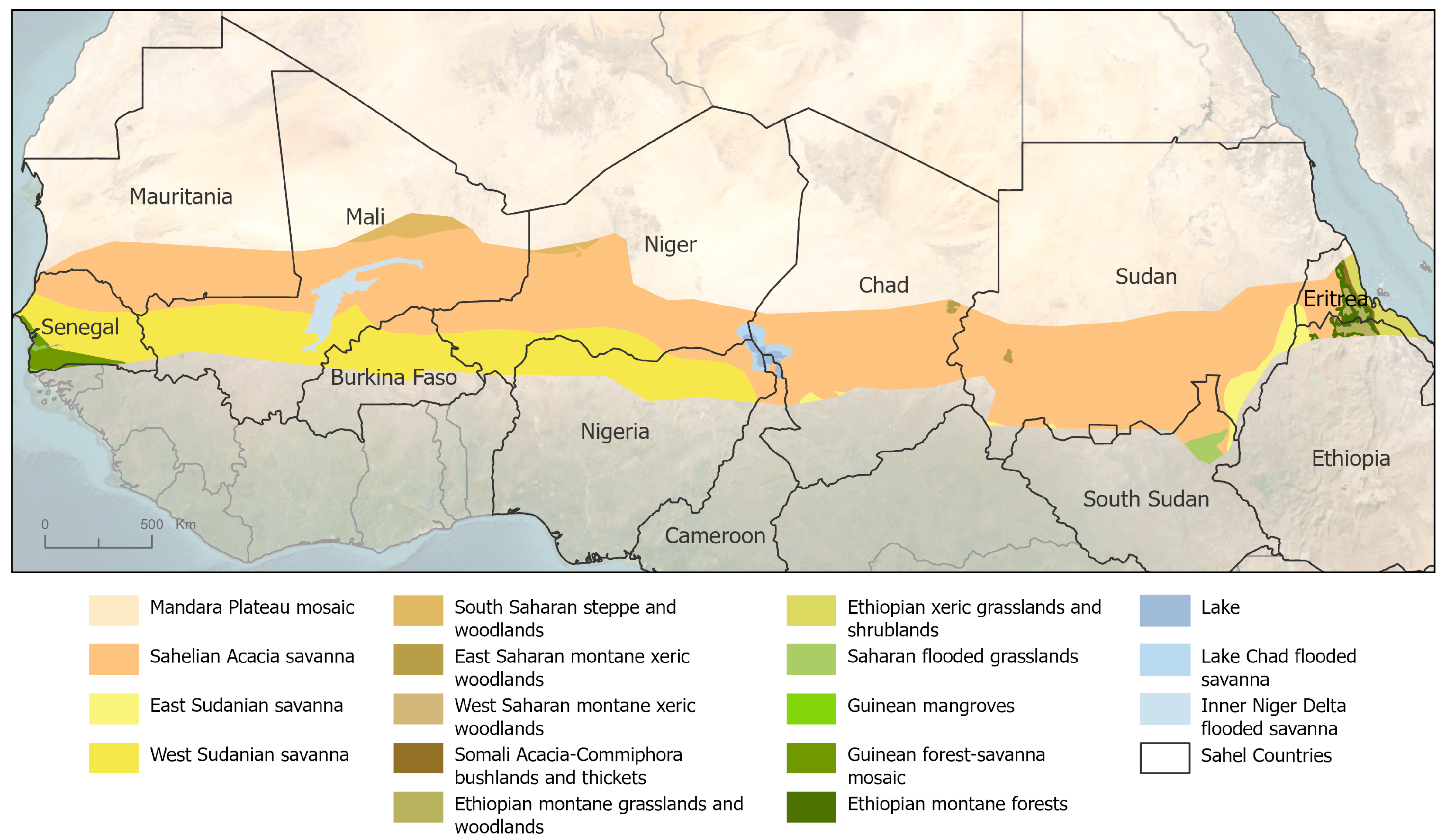
The Sahel region is a hot semi-arid area located just south of the Sahara Desert and north of the Sudanian savanna. It covers several countries, including Senegal, Mauritania, Mali, Burkina Faso, Niger, Nigeria, Chad, and Sudan (Figure 1). This region has a long, dry, and shorter rainy season, which spans approximately 8–9 months and 3–4 months, respectively [34]. In addition, rainfall distribution varies across the Sahel region, with higher precipitation in the southern areas when compared to the northern zones [35]. Lastly, recent studies have highlighted increased extreme rainfall over the past few years [7].

The Sahel encompasses a diverse array of terrestrial ecoregions [36], each presenting unique ecological characteristics and challenges, which have been considered while developing the proposed methodology (see Section 4).

Table 1. Ecoregions within the Sahel, with their respective areas, and the distribution of recorded flood events used for training and validation purposes.

Ecoregion	Code	km2 (% Sahel)	Num. Events Training	Num. Events Validation
Sahelian Acacia savanna	AT0713	2,234,057.9 (67.9)	523	57
West Sudanian savanna	AT0722	750,142.2 (22.8)	739	117
East Sudanian savanna	AT0705	60,353.6 (1.8)	0	0
Inner Niger Delta flooded savanna	AT0903	49,389.1 (1.5)	0	0
South Saharan steppe and woodlands	PA1329	47,839.7 (1.5)	0	0
Ethiopian xeric grasslands and shrublands	AT1305	32,501.1 (1.0)	0	0
Guinean forest-savanna mosaic	AT0707	28,863.5 (0.9)	0	0
Ethiopian montane forests	AT0112	22,347.5 (0.7)	0	0
Lake Chad flooded savanna	AT0904	17,827.4 (0.5)	20	2
Saharan flooded grasslands	AT0905	17,546.2 (0.5)	0	0
Ethiopian montane grasslands and woodlands	AT1007	15,156.4 (0.5)	0	0
East Saharan montane xeric woodlands	AT1303	4890.9 (0.1)	0	0
Somali Acacia-Commiphora bushlands and thickets	AT0715	4870.7 (0.1)	0	0
Guinean mangroves	AT1403	2251.8 (0.1)	2	0
West Saharan montane xeric woodlands	PA1332	201.2 (0.0)	0	0
Mandara Plateau mosaic	AT0710	107.6 (0.0)	0	0

provides a detailed breakdown of the ecoregions, the area they cover, and the total number of recorded flood events used in the study. This summary offers an overview of the spatial distribution of flood occurrences across different ecoregions.

Figure 1. Map of the Sahel region and its ecoregions, based on [37].

Figure 1. Map of the Sahel region and its ecoregions, based on [37].

Flood events have been documented across 91.3% of the Sahel, with the Sahelian Acacia savanna and West Sudanian savanna hosting most of these records. This reflects their extensive geographic coverage within the region and their susceptibility to flooding due to varying climatic and ecological conditions. These factors highlight the importance of tailoring methodologies to the unique characteristics of each ecoregion to enhance the results.

3. Datasets

For the data employed in this study, three main categories were considered: (i) ground truth, (ii) flood-related, and (iii) exposure-related data. Due to the scarcity of locally produced geospatial products in the Sahel, global datasets were selected as the only viable option (

Table 2. Datasets used in the study detailing their application, type, name, resolution, period, and source.

Use	Product Type	Dataset Name	Spatial Resolution	Period	Source (Accessed on 10 April 2024)
Ground Truth	Flood Events	DesInventar	Point	2015–2023	UNDRR (https://desinventar.cimafoundation.org/)
Flood-related	Precipitation	CHIRPS	5 km	2015–2023	UCSB (https://www.chc.ucsb.edu/data/chirps)
Flood-related	Soil Moisture	SMAP	9 km	2015–2023	NASA (https://smap.jpl.nasa.gov/data/)
Flood-related	Terrain	DEM	30 m	2011–2015	Copernicus (https://dataspace.copernicus.eu/explore-data/data-collections/copernicus-contributing-missions/collections-description/COP-DEM)
Exposure	LULC	World Cover	10 m	2020–2021	ESA (https://esa-worldcover.org/en)
Exposure	LULC	Dynamic Land Cover	100 m	2015–2019	Copernicus (https://land.copernicus.eu/en/products/global-dynamic-land-cover)
Exposure	Population	GHSL	100 m	2015 and 2020	JRC (https://data.jrc.ec.europa.eu/collection/ghsl)
Exposure	Buildings	OSM	Vector	2015–2023	OSM (https://www.openstreetmap.org/)
Validation	Buildings	Google (Open Buildings)	Vector	2016–2023	Open Buildings (https://sites.research.google/gr/open-buildings/)

).

3.1. Ground Truth

Data associated with flood events and their impacts (i.e., affected houses) were extracted from the DesInventar Sendai (https://desinventar.cimafoundation.org/ (accessed on 10 April 2024)), an open-source platform for disaster information management supported by the UNDRR. This platform was designed to address the scarcity of disaster data, particularly for smaller-scale events, via facilitating, storing, and analysing disaster-related information [38]. Compiling data on diverse disasters, DesInventar enhances the comprehension of disaster trends, refines prevention and mitigation measures, and makes informed decisions within the context of disaster risk management [39].

In this context, floods were found in various ecoregions within the Sahel, including the West Sudanian savanna, Lake Chad flooded savanna, Sahelian Acacia savanna, Ethiopian montane grasslands and woodlands, and the Guinean mangroves (Table 1). Notice that other data sources, such as EM-DAT (https://www.emdat.be/) [40] and the Copernicus Emergency Management Service (CEMS (https://emergency.copernicus.eu/)) [41], were also considered. However, the limited number of event records and the lack of detailed information on affected houses made us solely use the DesInventar database for this study.

3.2. Flood-Related Data

The utilized flood-related data included the Copernicus DEM (https://dataspace.copernicus.eu/explore-data/data-collections/copernicus-contributing-missions/collections-description/COP-DEM, accessed on 10 April 2024), CHIRPS (https://www.chc.ucsb.edu/data/chirps, accessed on 10 April 2024), and SMAP (https://smap.jpl.nasa.gov/data/, accessed on 10 April 2024) products. Using 30 m pixel spacing, the Copernicus DEM delineated the hydrological basins draining towards each flood location identified in the DesInventar database (see Section 4.1.2). In addition, the CHIRPS product, which is a daily precipitation dataset that integrates satellite imagery with in situ data from 1981 to the present for latitudes between 50°S and 50°N at a pixel resolution of 0.05 degrees [42], was used to extract the recorded precipitation before the flood events within the discharge basin. Lastly, the SMAP product, derived from NASA’s Soil Moisture Active Passive mission, was used to extract the soil moisture conditions in the discharge basin before each flood event. SMAP provides global soil moisture data within a 9 km pixel spacing and a 2–3 day revisit time, which allows us to understand the water content in the soil before the floods.

3.3. Exposure-Related Data

The exposure-related data used included the ESA’s WorldCover (https://esa-worldcover.org/en) and OSM (https://www.openstreetmap.org) to determine the number of houses at each flood-affected location. The ESA WorldCover is a detailed global product of land cover classes at 10 m for the years 2020 and 2021, which relies on Sentinel-1 and -2 images [43], while the OSM is a free and editable world map created and maintained by a community of volunteers where buildings are identified [44]. Additionally, the JRC’s Global Human Settlement Layer (GHSL) population grid product, which provides an estimation of the number of people living in each grid $100\times 100$ m cell of the world from 1975 to 2030 based on census data and information about built-up areas [45], was also used.

Additionally, the Open Buildings (https://sites.research.google/gr/open-buildings/, accessed on 10 April 2024) dataset [46], provided by Google, was used to support the validation of the results as an additional source of exposure data. This dataset provides information on the number of houses in the selected validation areas, allowing an assessment of the variance between the actual and predicted numbers of affected houses relative to the total number of houses in those areas. Note that this dataset was used only for validation rather than prediction, as it is limited to the African continent, and including it in the prediction process would restrict the applicability of the developed method to this region, even though its potential may be global.

4. Methods

The proposed methodology to predict the number of houses affected by floods as an SDG indicator has been developed to leverage a comprehensive set of existing datasets, integrating flood-related and exposure data (e.g., population and houses). Thus, the proposed algorithm operates through a structured workflow with three primary steps initiated after the user selects the AOI. The steps are (i) data extraction (i.e., ground truth, flood-related, and exposure), (ii) model training, and (iii) validation. These steps are outlined in the simplified structure presented in Figure 2. The following subsections provide a detailed explanation of each stage.

4.1. Data Extraction

The data extraction step involved collecting and organizing diverse datasets. This section describes the sources and handling of the ground truth, flood-related, and exposure data.

4.1.1. Ground Truth

The algorithm has been designed to operate at the municipality level due to the unavailability of more detailed data such as neighborhoods or streets. The data were filtered and grouped to address data duplication in the DesInventar dataset, which often reported single events multiple times due to their varying impacts across different parts of a municipality. This process ensured the removal of redundant records. Regarding the impacts of flood events, the DesInventar database provides detailed information on human and material losses. For the most recent data, it documents the number of houses destroyed and affected. Only the aggregated figures for affected houses were considered to simplify the algorithm. This approach consolidates all material impacts (i.e., including destroyed houses) under the category of affected houses.

Finally, the DesInventar database did not provide latitude and longitude information for the events. Therefore, extracting these coordinates from additional sources was necessary. Specifically, using data from Wikidata, Wikipedia’s central data management platform and a data source also used in previous EO-based studies [47]. Wikidata is highly interlinked and connected to many other datasets, making it a valuable resource [48]. To improve spatial accuracy, the extracted coordinates were cross-referenced with OpenStreetMap (OSM) land use data to ensure that they overlapped with known settlement areas, thereby reducing the potential for misalignment between flood locations and exposure inputs.

The following example from the DesInventar database illustrates the data considered for extracting the labels of affected houses, which were used to train and validate the algorithm (

Table 3. Example of the DesInventar data considered as Ground Truth.

Department	Region	Location	Date 1	Latitude 2	Longitude 2	Affected Houses
Zinder	Dungass	Malawa	20190729	13.03°	9.61°	0
Maradi	Tessaoua	Ourafane	20200715	14.07°	8.13°	68
Tillaberi	Kollo	Liboré	20200813	13.4°	2.19°	0
Zinder	Mirriah	Mirriah	20200917	13.71°	9.16°	28
Tahoua	Madaoua	Azarori	20200613	14.14°	5.9°	0
Zinder	Matamaye	Kantche	20190618	13.54°	8.46°	54
Dosso	Birningaoure	Kiota	20160802	13.29°	2.96°	1

¹ Note that Date is in YYYYMMDD format. ² Note that latitude and longitude are expressed in the EPSG:4326 coordinate system.

). Notice that the sample events in the Table were selected randomly.

4.1.2. Flood-Related Data

To evaluate the hydrological context of each flood event, the watershed draining into each affected location was delineated using the Copernicus DEM as input data and processed with WhiteboxTools v2.3 (https://www.whiteboxgeo.com/manual/wbt_book/preface.html, accessed on 10 April 2024) [49]. This watershed delineation was needed to analyze flow dynamics and potential flood impacts.

Accumulated precipitation and soil moisture data, derived from CHIRPS and SMAP products, respectively, were extracted for the month preceding each flood event. These data were categorized into four temporal intervals: 0–7, 7–14, 14–21, and 21–28 days before the official flood date (

Table 4. Flood-related considered inputs.

Variable	Short Name
Rainfall (mm, CHIRPS): 0–7 days before event	Rain_0_7
Rainfall (mm, CHIRPS): 7–14 days before event	Rain_7_14
Rainfall (mm, CHIRPS): 14–21 days before event	Rain_14_21
Rainfall (mm, CHIRPS): 21–28 days before event	Rain_21_28
Soil moisture (wfv, SMAP): 0–7 days before event	SoilM_0_7
Soil moisture (wfv, SMAP): 7–14 days before event	SoilM_7_14
Soil moisture (wfv, SMAP): 14–21 days before event	SoilM_14_21
Soil moisture (wfv, SMAP): 21–28 days before event	SoilM_21_28

Note that wfv means water fraction by volume.

). The 7-day window was selected to reflect the rapid hydrological response typical of arid and semi-arid regions, where short, intense rainfall over low-infiltration soils generates rapid run-off and flash flooding. These conditions often produce sharp hydrographs with rising limbs and peak flows shortly after precipitation events, making short-term antecedent conditions particularly relevant [5]. Thus, the combination of accumulated rainfall and soil moisture influences run-off generation and soil infiltration, and, as such, these determine the magnitude of floods.

4.1.3. Exposure Data

Exposure data, including building areas, urban area extent, and population within affected locations, were extracted from (i) OpenStreetMap (OSM), (ii) Land Use Land Cover (LULC) data, (iii) and the Global Human Settlement Layer (GHSL), respectively. OSM provided building area data, LULC offered urban area extent, and GHSL supplied population distribution estimates.

To further refine the exposure assessment, the flood potential classification method proposed by Wang and Liu [50] was employed, which involves calculating a flood order from a DEM that ranks grid cells based on their elevation and proximity to water bodies. By statistically analyzing these flood order values, the areas were categorized into four flood potential classes: (i) very low, (ii) low, (iii) medium, and (iv) high.

Table 5. Exposure data considered inputs.

Variable	Short Name
Population (GHSL) in Very Low flood potential areas	Pop_VL
Population (GHSL) in High flood potential areas	Pop_H
Population (GHSL) in Medium flood potential areas	Pop_M
Population (GHSL) in Low flood potential areas	Pop_L
Building Area (sqm, OSM) in Very Low flood potential areas	BldgArea_VL
Building Area (sqm, OSM) in High flood potential areas	BldgArea_H
Building Area (sqm, OSM) in Medium flood potential areas	BldgArea_M
Building Area (sqm, OSM) in Low flood potential areas	BldgArea_L
Urban Area (ha, LULC) in Very Low flood potential areas	UrbArea_VL
Urban Area (ha, LULC) in High flood potential areas	UrbArea_H
Urban Area (ha, LULC) in Medium flood potential areas	UrbArea_M
Urban Area (ha, LULC) in Low flood potential areas	UrbArea_L

presents the exposure data (i.e., building area, urban area extent, and population) extracted for each flood potential category. Notice that efforts were made to extract the flooded area using Sentinel-1 and Sentinel-2 observations. However, the rapid nature of the recorded floods, which did not coincide with the acquisition times of the satellites, limited the potential of satellite imagery to capture the true extent of the affected areas for each event.

4.2. Model Training

To establish a robust training dataset of flood events using DesInventar records, pinpointing their exact location and date were necessary. Relevant flood-related data (see Section 4.1.2) and exposure data (see Section 4.1.3) were extracted for each event. These data were then integrated with the number of affected houses, sourced from DesInventar (see Section 4.1.1), resulting in a comprehensive dataset (

Table 6. Example of a comprehensive dataset used for training the machine learning model, showcasing five flood events.

Location	Chetimari	Goudoumaria	Gadabedji	Tabalak	Ouallam
Date	15/10/2019	12/07/2018	25/08/2019	05/07/2017	23/08/2020
Affected Houses	768	45	26	36	51
Latitude 1	13.2°	13.7°	15.0°	15.1°	14.3°
Longitude 1	12.4°	11.2°	7.2°	5.7°	2.1°
Rain_0_7 (mm)	4.8	10.6	16.5	2.5	48.0
Rain_7_14 (mm)	4.3	10.6	9.0	6.3	15.0
Rain_14_21 (mm)	3.8	18.1	9.3	0.3	56.3
Rain_21_28 (mm)	0.0	10.6	8.2	3.5	30.0
SoilM_0_7 (wfv)	0.1	0.1	0.1	0.1	0.2
SoilM_7_14 (wfv)	0.1	0.1	0.1	0.1	0.2
SoilM_14_21 (wfv)	0.1	0.1	0.1	0.1	0.2
SoilM_21_28 (wfv)	0.1	0.0	0.1	0.1	0.2
Pop_VL (population)	970	6059	5150	1431	10,580
Pop_L (population)	1067	1713	6523	3267	11,665
Pop_M (population)	325	7595	6887	303	3874
Pop_H (population)	34	1104	3479	0	0
BldgArea_VL (sqm)	20,748.0	12,679.2	2837.5	5164.6	9923.6
BldgArea_L (sqm)	1046.5	625.4	1909.0	4341.6	3300.8
BldgArea_M (sqm)	105.2	825.0	2205.1	0.0	0.0
BldgArea_H (sqm)	0.0	74.3	1387.7	0.0	0.0
UrbArea_VL (ha)	12.1	16.1	0.0	2.9	57.7
UrbArea_L (ha)	0.9	0.9	0.0	3.1	30.4
UrbArea_M (ha)	0.0	2.0	0.0	0.0	7.6
UrbArea_H (ha)	0.0	0.0	0.0	0.0	0.0

¹ Please note that latitude and longitude values have been rounded to one decimal place and are expressed in the EPSG:4326 coordinate system.

). Thus, such a dataset was used to train different random forest regressors [51], one for each ecoregion, capable of predicting the affected houses by floods. Notice that ‘random forests’ is a machine learning model well-known for its robustness to noisy data [52,53] and its resistance to over-fitting. This study used the events from 2015 to 2020 for training and events from 2021 to 2023 for validation.

4.3. Validation

Once the random forest models were trained, the number of houses affected by floods was estimated, which will serve as an estimator of the SDG indicator, using flood-related data (see Section 4.1.2) and exposure data (see Section 4.1.3) for a given location. To evaluate these predictions, the estimated figures for affected houses were validated by comparing the predicted values with the actual data obtained from specific flood events selected for validation purposes (Table 1). The validation entailed analyzing the absolute and relative errors between the predicted and observed values. Thus, the validation of absolute values involved a direct comparison between the predicted number of affected houses and the actual number recorded in the validation dataset. On the other hand, the relative assessment examined the proportion of predicted affected houses relative to the total number of houses in the location, compared to the actual proportion of affected houses. For this purpose, the total number of houses was derived from the Open Buildings dataset provided by Google.

RMSE, a reliable measure of the algorithm performance, provided an average value of the differences between the predicted and actual outputs and was employed as a primary metric to evaluate the predictive performance of the models (Equation (1)). In addition, to quantify prediction uncertainty, bootstrap resampling (10,000 iterations) was used to derive 95% confidence intervals for the mean prediction error across ecoregions.

$$\mathrm{RMSE}=\sqrt{{\displaystyle \frac{1}{n}}\sum _{i=1}^n{(y_i-{\widehat{y}}_i)}^2}$$

(1)

where, $y_i$ and ${\widehat{y}}_i$ represent the actual and predicted values while n is the total number of observations. This metric quantifies the accuracy of the algorithm across different ecoregions, highlighting its strengths and limitations. Furthermore, to enhance model interpretability, both the relative input importance from the random forests and SHAP (SHapley Additive exPlanations) values were computed, allowing a more transparent assessment of trained models.

5. Results

The estimation of affected houses was validated by comparing predicted values with actual outputs for flood events set aside expressly for validation. This comparison provides insights into the predictions’ absolute and relative accuracy. Additionally, it underscores the significance of input data quality in forecasting the extent of affected houses. The following sections present detailed results and analysis of these predictions.

5.1. Prediction Accuracy

The prediction accuracy for the number of houses affected by floods varies notably across different ecoregions. The Lake Chad flooded savanna demonstrates the highest prediction accuracy, with the lowest RMSE value of 73.33. In contrast, predictions for the Sahelian Acacia savanna and West Sudanian savanna show higher RMSE values (136.84 and 130.84, respectively), indicating more significant errors and potential challenges in modeling flood impacts accurately in these regions (

Table 7. RMSE of Predicted vs. Actual number of houses affected by floods, grouped by ecoregions with validation records.

Ecoregion	RMSE
Sahelian Acacia savanna (AT0713)	136.84
West Sudanian savanna (AT0722)	130.84
Lake Chad flooded savanna (AT0904)	73.33

).

In the Lake Chad flooded savanna, the algorithm achieves its best accuracy in events where more than 100 houses are affected, as indicated by the consistent RMSE of around 73.33. However, only two validation events were available for such an ecoregion, which may restrict the validation (Figure 3c). For the Sahelian Acacia savanna, prediction error varies significantly, with the highest RMSE of 202.04 seen in the group affecting over 100 houses. Meanwhile, smaller-scale events affecting 11–50 houses had an RMSE of 77.17. While this suggests reasonable performance, the error appears relatively high, given the limited scale of these events. This fluctuation indicates that the algorithm struggles with larger-scale flood events in this region and exhibits notable errors for smaller ones (Figure 3a). A similar trend is observed in the West Sudanian savanna, where RMSE peaks at 241.13 for small-scale events and rises again to 141.33 for the largest impact group. However, the algorithm demonstrates its highest accuracy for medium-sized events (51–100 affected houses), with a significantly lower RMSE of 42.92. These results suggest that prediction accuracy in the West Sudanian savanna is most reliable for moderate-scale events, while both small and large-scale cases exhibit greater uncertainty (Figure 3b). However, it is essential to note that the error is also influenced by the total number of houses in each location, not just the number of affected houses.

Regarding the differences between actual and predicted values for each event, the algorithm displayed both overestimation and underestimation instances in predicting the number of affected houses. Some misalignments between actual and predicted values were observed in the Sahelian Acacia savanna (Figure 4a). While the algorithm performed well for many events, accurately aligning predictions with actual data, challenges arose in some instances, particularly for larger-scale flood events. The most significant discrepancy occurred in an event where 670 affected houses were recorded, yet the algorithm estimated only 66, highlighting an underestimation. The algorithm showed mixed performance in the West Sudanian savanna (Figure 4b). It achieved relatively accurate predictions for certain moderate-impact events but struggled considerably when faced with events of higher extremes. This inconsistency is evident in several cases where the algorithm markedly over- or under-predicted the number of affected houses, suggesting significant challenges in handling events characterized by high variability or magnitude. Only two events were available for validation in the Lake Chad flooded savanna ecoregion (Figure 4c). In both cases, the algorithm underestimated the number of affected houses. However, these differences were less pronounced than some errors observed in the Sahelian Acacia and West Sudanian savannas. Nevertheless, the limited number of validation events in this ecoregion restricts the reliability of the results, as the small sample size may not adequately reflect the overall predictive capability.

To assess the reliability of the prediction error estimates, 95% confidence intervals for the mean prediction error were calculated using bootstrap resampling (10,000 iterations) (

Table 8. Mean prediction error and 95% confidence intervals for each ecoregion, based on bootstrap resampling (10,000 iterations).

Ecoregion	Mean Error (Houses)	95% CI
Sahelian Acacia savanna (AT0713)	35.21	(2.75, 72.21)
West Sudanian savanna (AT0722)	51.46	(29.27, 72.74)
Lake Chad flooded savanna (AT0904)	−73.00	(−80.00, −66.00)

). Thus, the West Sudanian savanna (AT0722) and Sahelian Acacia savanna (AT0713) exhibited positive mean errors of 51.46 and 35.21, respectively, with upper confidence bounds exceeding 70 houses. In contrast, the Lake Chad flooded savanna (AT0904) showed a negative mean error of −73.00, with a relatively narrow confidence interval of (−80.00, −66.00). These results are consistent with the observed patterns in Figure 5, where the prediction accuracy was higher in AT0904, though based on a smaller validation sample.

However, these differences are not substantial when considering the total number of houses exposed in each event (Figure 6). The percentage differences between the predicted and actual values of affected houses in the three ecoregions reveal that the medians of each distribution are close to zero, indicating that the predictive models generally achieve satisfactory accuracy. Specifically, in the Lake Chad flooded savanna ecoregion (AT904), the interquartile range (IQR) is relatively narrow, reflecting a high degree of consistency in predictions. However, this is likely influenced by the limited sample size of only two observations. In contrast, the West Sudanian savanna (AT0722) and the Sahelian Acacia savanna (AT0713) regions showed wider IQRs, highlighting greater variability and reduced accuracies in the predictions, which is expected, given the more significant number of validation events (117 and 57, respectively). Notably, both the Sahelian Acacia savanna and the West Sudanian savanna show a slight overestimation trend of affected houses in the predictions compared to the actual values. Despite some outliers and variability, the overall differences remain within a reasonable range, predominantly between −2% and 3%. This modest variation suggests that the predictive performance of the algorithm is robust, particularly given the considerable scale of the events and the extensive number of houses at risk in the Sahel region.

5.2. Inputs Importance

The relative importance of the flood-related and exposure data used to predict the number of affected houses was analyzed by using the random forests trained models since, during the training process, the importance of each input when predicting the affected houses was computed for each ecoregion (Figure 7). Thus, these results indicate that rainfall data and soil moisture are among the most influential inputs, followed by urban area, building area, and population metrics.

To enhance interpretability and address the limitations of standard feature importance rankings, SHAP values were also computed for each ecoregion to provide a more robust and model-agnostic assessment of input influence. The SHAP summary plots (Figure 8) reveal the direction and magnitude of each feature’s contribution to the predicted number of affected houses. In addition to reaffirming the key role of rainfall and soil moisture predictors, SHAP values highlight important non-linear and interaction effects, particularly in relation to built-up area and flood potential indicators. These results further corroborate the findings from the original importance analysis, while offering more transparent insights into the prediction logic of the trained models.

However, differences regarding input importances among the ecoregions can be found. In the Lake Chad flooded savanna (AT0904), soil moisture data recorded between 7 and 14 days before each flood event plays the most critical role, contributing to over 40% of the importance of the models. This suggests that pre-flood moisture conditions significantly influence the flood impact in this region, where saturated soils may exacerbate flooding severity. Rainfall occurring 0–7 days before each flood event also holds notable importance, reflecting the immediate trigger for flood occurrences in this ecoregion. These patterns were reaffirmed by the SHAP analysis, which showed concentrated and consistently positive SHAP values for these predictors.

For the West Sudanian savanna (AT0722), building areas in high flood potential zones emerge as the most significant predictor, accounting for approximately 30% of the total importance. This highlights the vulnerability of infrastructure in areas prone to flooding. SHAP values, likewise, emphasized the high contribution of urban exposure variables, particularly when combined with elevated rainfall inputs in the week preceding the event. Additionally, rainfall recorded 0–7 days before an event is another key driver, underscoring the direct relationship between recent precipitation and flood impact in this region.

Finally, in the Sahelian Acacia savanna (AT0713), the model attributes the highest importance to soil moisture levels measured 14–21 days before an event (approximately 20%), followed by soil moisture levels recorded 0–7 days before the flood. This pattern indicates that moisture conditions play a role in shaping flood dynamics in this region.

6. Discussion

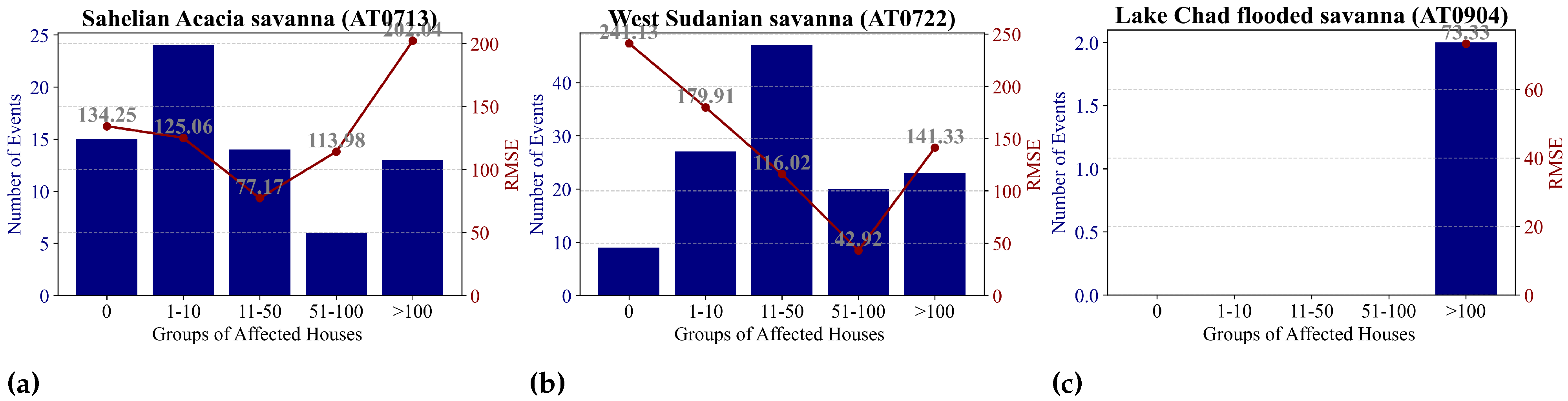
The results of this study offer critical insights into the performance of an algorithm for estimating the number of houses affected by flood events across different ecoregions within the Sahel. The observed variability in prediction accuracy, characterized by discrepancies between predicted and actual outputs, aligns with prior research that highlights the challenges of modeling complex and dynamic flood phenomena, particularly in data-scarce regions such as the Sahelian and West Sudanian savannas [54]. Studies have shown that landscape heterogeneity, floodplain complexity, and inconsistent data availability often increase prediction errors, as seen in the high RMSE values reported in these regions. The Lake Chad flooded savanna, demonstrating the highest prediction accuracy, underscores the impact of simplified conditions or limited validation datasets. While the RMSE of 73.33 suggests robust algorithm performance, this result should be interpreted cautiously. The limited number of events in this ecoregion (only two) may not adequately reflect the range of flood scenarios, potentially inflating the perceived accuracy. This region’s relatively homogeneous landscape and flat floodplain conditions may also simplify the flood modeling process, as fewer environmental variables introduce uncertainty. Nonetheless, this result highlights the potential benefits of focused datasets in improving predictive reliability when applied in regions with consistent environmental characteristics. Comparatively, the Sahelian Acacia savanna and West Sudanian savanna exhibited more pronounced errors, with RMSE values of 136.84 and 130.84, respectively. This finding suggests that the models struggle to accurately capture the nuances of larger-scale flood events, consistent with hypotheses from earlier studies that emphasise the importance of detailed topographic and hydrologic data for flood prediction in complex terrains. The higher variability in these regions may arise from their more heterogeneous landscapes, characterized by a mixture of dry lands, variable soil infiltration rates, and complex hydrological pathways. This aligns with findings from prior studies that highlight the role of terrain complexity and data quality in influencing flood prediction accuracy [55].

The analysis of affected houses reveals a clear trend: the prediction accuracy of the algorithm is closely linked to the scale of the flood impact, with accuracy decreasing as the scale of impact increases. Smaller-scale flood events, such as those affecting 11–50 houses, were predicted with relatively low RMSE values, particularly in the Sahelian Acacia savanna (RMSE = 77.17) and West Sudanian savanna (RMSE = 42.92 for events impacting 51–100 houses). These findings align with the observed bias in the training dataset, where moderate-impact events (11–100 affected houses) were better represented, particularly in regions like AT0722 and AT0713. Conversely, the algorithm exhibited significant underperformance for extreme flood events, with RMSE values exceeding 200 when the number of affected houses surpassed 100, likely due to their sparse representation in the training data (e.g., only 60 cases in AT0713 and 79 cases in AT0722 for events >100 houses). This emphasizes the accuracy dependency on the similarity between the predicted events and the distribution of events used in training, with models performing best for scenarios resembling the most frequent and moderately impactful floods within the training dataset. Additionally, fixed aggregation windows may also limit the ability of the algorithm to capture delayed hydrological responses or longer-term flood generation processes since flood dynamics are often shaped by both immediate and antecedent hydrological conditions, which can vary substantially across regions and years [5].

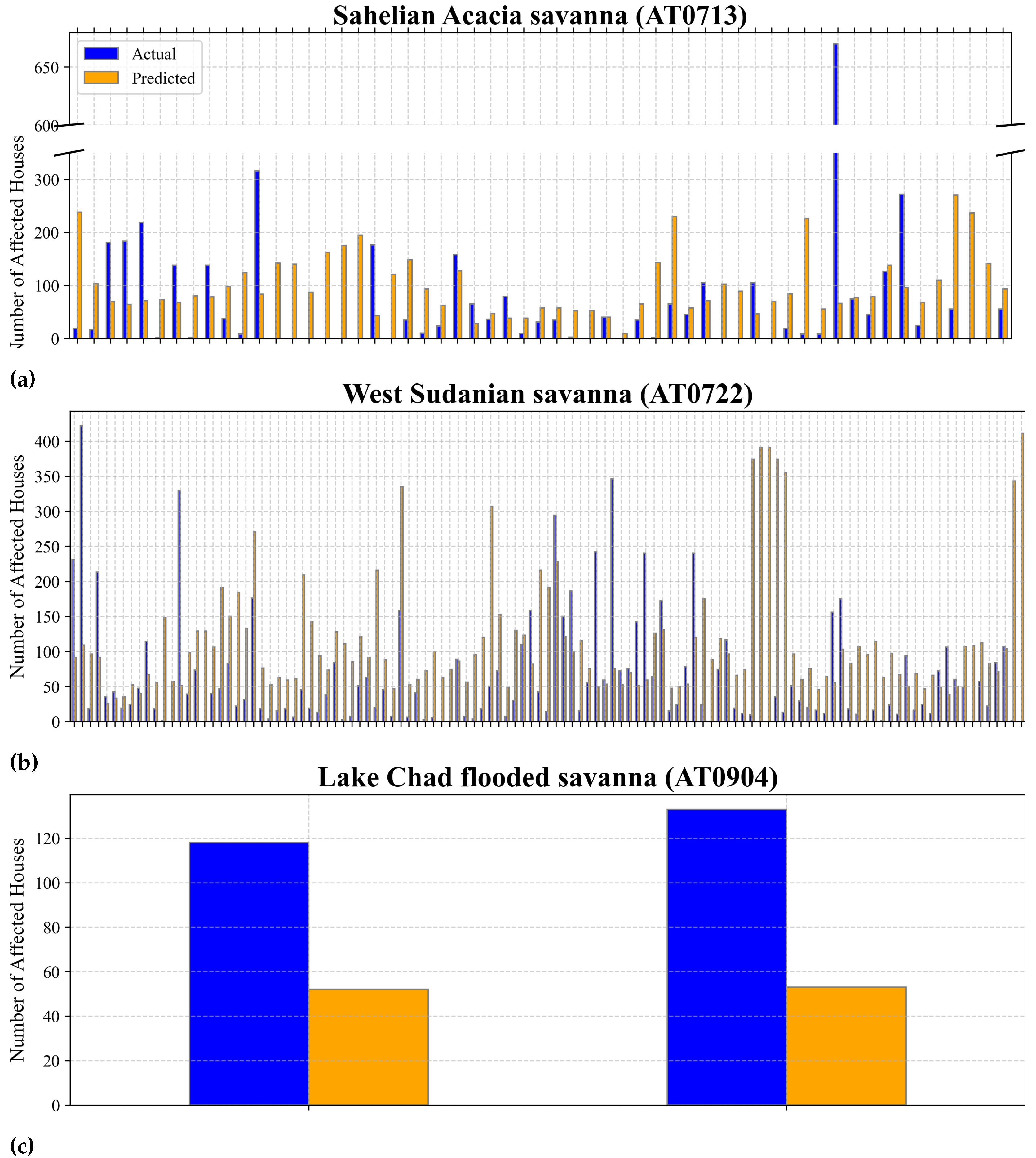
The consistent patterns of overestimation and underestimation observed in certain regions, particularly in the Sahelian Acacia savanna, suggest the presence of systemic biases in the predictive models. A notable example is the substantial discrepancy in an event where the number of affected houses was 670, but the algorithm estimated only 66, highlighting a severe underestimation issue. This underperformance is likely exacerbated by the scarcity of extreme events (e.g., those affecting >600 houses) in the training dataset, with only eight such cases in AT0713, six in AT0722, and none in AT0904. The lack of sufficient training data for large-scale floods impedes the ability of the algorithm to predict high-impact events, which deviate significantly from the more frequent, moderate-impact scenarios that dominate the training set.

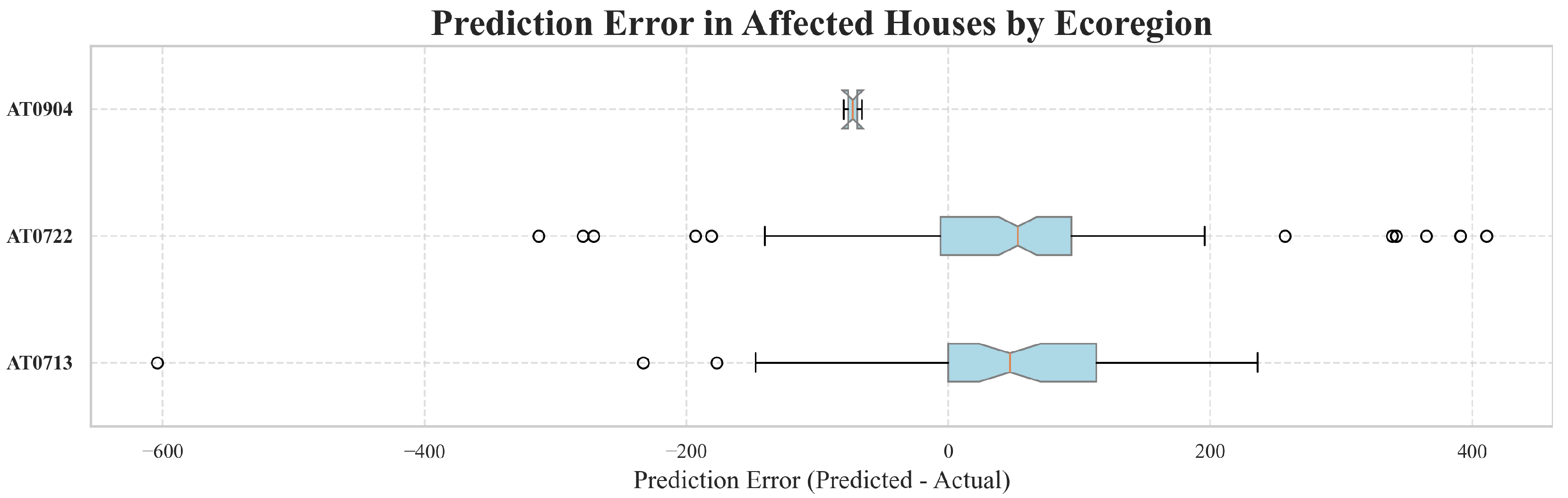
The findings reveal that, despite some variability, the algorithm demonstrates a robust ability to estimate the percentage of affected houses when considering the total number of exposed houses in each location across different ecoregions, which is a key achievement of this research. The percentage differences between predicted and actual values in all three ecoregions are close to zero, indicating satisfactory overall accuracy. Notably, the Lake Chad flooded savanna (AT0904) exhibits a narrow IQR, reflecting consistent predictions, though the limited sample size likely influences this consistency. In contrast, the Sahelian Acacia savanna (AT0713) and West Sudanian savanna (AT0722) regions show more significant variability, with wider IQRs due to the larger number of validation events. While these regions experience a slight trend of overestimating affected houses, the differences are generally modest, ranging between 2% and 3% of under- and overestimation, respectively, even for large-scale events involving extensive numbers of houses. This ability to accurately predict the percentage of affected houses holds significant practical implications, especially in improving resilience to floods in the Sahel and surrounding regions, where extreme rainfall and flooding events are becoming increasingly frequent. By providing reliable estimates of the proportion of houses affected, authorities can better anticipate the potential number of impacted individuals and initiate timely mitigation measures. This predictive capability enables more effective planning for disaster response, resource allocation, and long-term adaptation strategies, ultimately reducing the adverse impacts of floods on vulnerable communities.

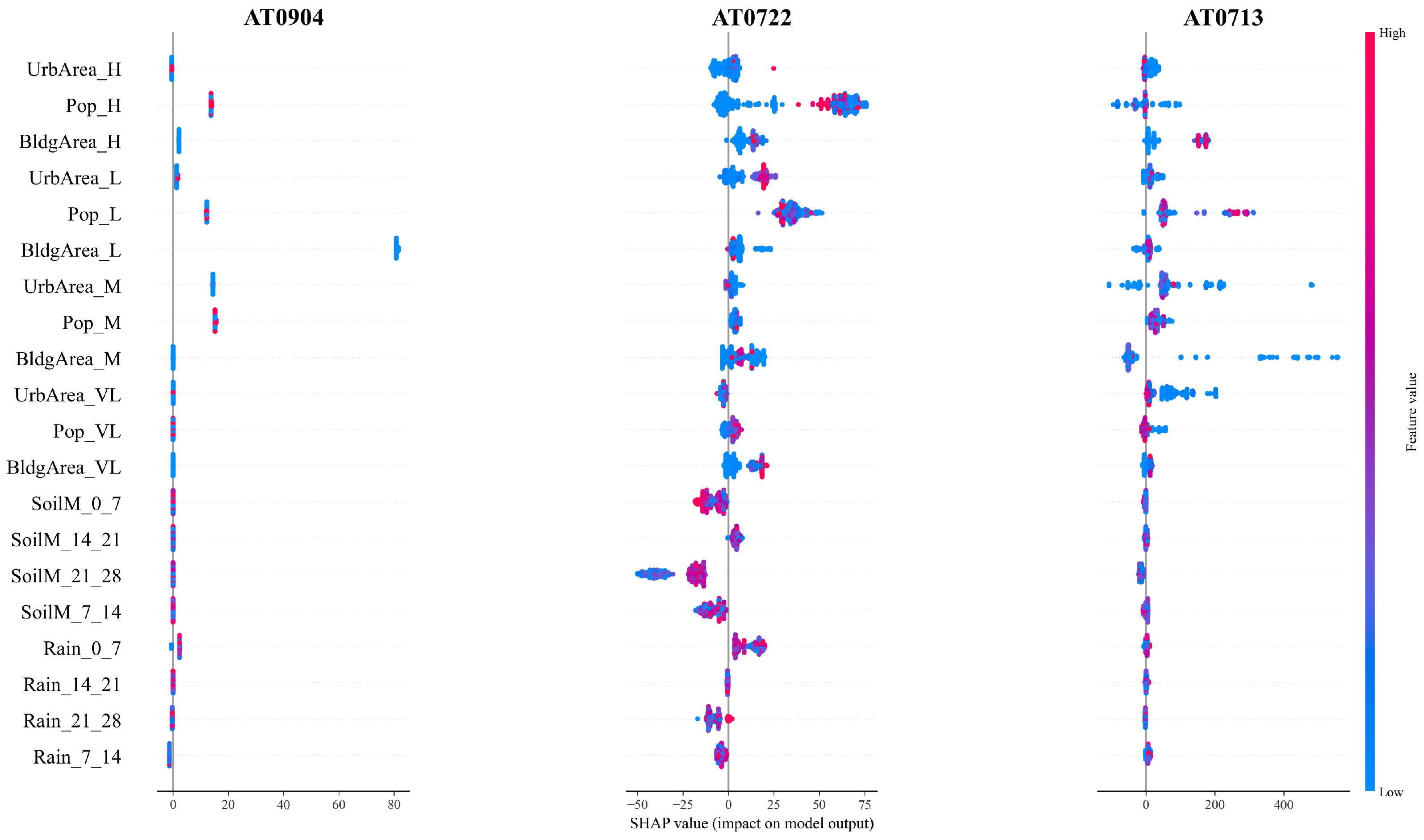
In order to improve interpretability and transparency of model behavior, SHAP values were also employed to decompose the contribution of each input to individual predictions. These results corroborate the variable importance rankings derived from the random forest algorithm while enabling a more granular assessment of local feature effects. Notably, the SHAP analysis highlights the heterogeneous influence of predictor variables across ecoregions, reinforcing the importance of regionally adaptive modeling strategies. The inclusion of SHAP values aligns with best practices in explainable machine learning and enhances the transparency and policy relevance of the model, particularly in the context of decision-making for flood risk mitigation. Nevertheless, the current approach has not yet been validated on out-of-sample regions, and no direct comparison has been made with physically based hydrodynamic models such as LISFLOOD [56]. Such models require detailed hydraulic and structural data that are currently unavailable for the Sahel. Future research should consider hybrid approaches and cross-validation with physical models to enhance robustness and assess generalizability under varying geographic and hydrological conditions.

On the other hand, the analysis of input variable importance further reinforces the need for high-quality input data tailored to regional conditions to improve predictive accuracy and guide future model enhancements. Across all three ecoregions, soil moisture and rainfall data emerged as the most influential predictors, highlighting the central role of meteorological and hydrological conditions in shaping flood impacts. Pre-event soil moisture levels in the Lake Chad flooded savanna were particularly critical, likely due to the flat terrain’s propensity to exacerbate flooding under saturated conditions [57]. Similarly, in the West Sudanian savanna, building area and infrastructure metrics were highly significant, reflecting the vulnerability of human settlements in flood-prone zones. These findings demonstrate the reliance of the algorithm on specific input variables and emphasize the importance of integrating diverse and reliable data sources. However, several critical variables such as building materials, detailed elevation data, and drainage infrastructure were not included due to their unavailability at the required spatial resolution or coverage across the study area [58].

To further quantify prediction reliability, 95% confidence intervals for the mean prediction error were computed via bootstrap resampling (10,000 iterations). These intervals provide a quantitative measure of uncertainty and highlight the variability in accuracy across ecoregions. The Sahelian Acacia savanna (AT0713) and West Sudanian savanna (AT0722) showed wider confidence bounds, indicating greater uncertainty due to complex terrain and more diverse event samples. Conversely, the Lake Chad flooded savanna (AT0904) exhibited a narrow interval, reflecting lower observed error given the inflated confidence due to the limited validation sample.

In line with the methodological direction of the present study, related work by Marín-García et al. (2023) [59] employed decision tree algorithms to classify building damage levels resulting from riverine floods in the Andalusia (Spain). Their approach, which relied on a relatively limited dataset and environmental predictors, achieved a classification accuracy of 81.09% (±13.77%) across three predefined damage categories. Such work illustrates the growing emphasis on operationally feasible methods in flood impact assessment where data are lacking. Against this backdrop, the RMSE values reported in the present study (ranging from 73 to 137) may be considered consistent with expectations, underscoring the reliability and suitability of the algorithm for application in regions characterized by limited observational records and heterogeneous infrastructure data, such as the Sahel.

Although the random forest algorithm was selected due to its established performance with limited and imbalanced datasets, its resilience to overfitting, and its ability to provide interpretable outputs through variable importance measures [52], it is recognized that alternative modeling techniques such as XGBoost, support vector machines, or deep learning models may offer advantages under different conditions. However, these methods typically require larger datasets to perform effectively. In particular, deep learning approaches have shown considerable potential in flood prediction when applied to large-scale and high-frequency datasets [60], which are not available in the Sahel. XGBoost, although effective in other flood susceptibility assessments also benefits from larger training data [61]. Given the data-scarce nature of the current study area, random forest was deemed the most appropriate method. Nonetheless, future research should explore these alternatives as more extensive and detailed datasets become available, to assess potential improvements.

Finally, the methodology developed in this study is readily adaptable to other data-scarce, flood-prone regions beyond the Sahel. Its reliance on globally available datasets such as CHIRPS for precipitation, SMAP for soil moisture, GHSL for population, and OpenStreetMap for exposure ensures broad applicability. By recalibrating the algorithm using locally observed flood events and tailoring the ecological stratification to reflect regional hydrological and environmental conditions, this framework can be extended to diverse contexts including parts of Southeast Asia, Central America, and East Africa. Such an adaptation would allow local authorities in similarly vulnerable regions to utilize low-cost and open-access data for flood resilience planning and the effective monitoring of SDG Indicator 13.1.1.

7. Conclusions

This study provides insights into the performance of predictive models for estimating the number of houses affected by flood events across distinct ecoregions in the Sahel. While the results reveal a satisfactory level of accuracy overall when considering the total number of exposed houses in each location, with percentage differences between predicted and actual values close to zero in most cases, the variability in prediction accuracy across regions and scales underscores key challenges. Smaller-scale floods were generally predicted with higher accuracy, reflecting biases in the training dataset, favoring moderate-impact events. However, the algorithm struggled with extreme flood events, particularly those affecting over 600 houses, due to their under-representation in the training data.

Additionally, the ability of the algorithm to accurately estimate the percentage of affected houses has significant practical implications. Reliable percentage predictions enable authorities to better anticipate the number of affected individuals, facilitating more efficient disaster response, resource allocation, and mitigation planning. As extreme rainfall and flood events are expected to become more frequent in the Sahel, this capability will enhance regional resilience.

In addition, the analysis of input variable importance underscores the central role of high-quality, region-specific data in improving model performance. Meteorological and hydrological variables, particularly soil moisture and rainfall, emerged as the most influential predictors, while infrastructure metrics were significant in densely populated regions. Notably, the accurate prediction of the number of affected houses can serve as a critical SDG indicator, aligning with global objectives to enhance climate resilience and mitigate the impacts of disasters.

Finally, future research should focus on overcoming key data limitations and tailoring models to specific regional contexts. The current study relied on openly available datasets, which, while enabling broad applicability, constrained the inclusion of critical variables such as building materials, drainage infrastructure, and high-resolution elevation data. Modeling choices were guided by the nature of the available data, with random forest preferred for its interpretability and suitability for small, imbalanced datasets; however, comparative evaluation with alternative algorithms remains a priority for future research. Furthermore, the geographic focus on the Sahel, though highly relevant, constrains the assessment of generalizability beyond this region. To address these challenges, future work should explore cross-regional validation, incorporate finer-grained socio-environmental inputs, and consider simulating synthetic extreme scenarios to compensate for the under-representation of high-impact events in historical records. These efforts will enhance predictive accuracy and support broader objectives of building resilience, protecting livelihoods, and reducing community vulnerability to increasingly severe flood events.

References

1. Parmesan, C.; Morecroft, M.D.; Trisurat, Y. Climate Change 2022: Impacts, Adaptation and Vulnerability. Ph.D. Thesis, GIEC, Geneva, Switzerland, 2022. [Google Scholar]
2. Caloiero, T. Hydrological Hazard: Analysis and Prevention; MDPI: Basel, Switzerland, 2018. [Google Scholar]
3. Coly, S.M.; Zorom, M.; Leye, B.; Karambiri, H.; Guiro, A. Learning from history of natural disasters in the Sahel: A comprehensive analysis and lessons for future resilience. Environ. Sci. Pollut. Res. 2024, 31, 40704–40716. [Google Scholar] [CrossRef] [PubMed]
4. Rentschler, J.; Salhab, M.; Jafino, B.A. Flood exposure and poverty in 188 countries. Nat. Commun. 2022, 13, 3527. [Google Scholar] [CrossRef] [PubMed]
5. Elagib, N.A.; Zayed, I.S.A.; Saad, S.A.; Mahmood, M.I.; Basheer, M.; Fink, A.H. Debilitating floods in the Sahel are becoming frequent. J. Hydrol. 2021, 599, 126362. [Google Scholar] [CrossRef]
6. Chagnaud, G.; Panthou, G.; Vischel, T.; Lebel, T. A synthetic view of rainfall intensification in the West African Sahel. Environ. Res. Lett. 2022, 17, 044005. [Google Scholar] [CrossRef]
7. Biasutti, M. Rainfall trends in the African Sahel: Characteristics, processes, and causes. Wiley Interdiscip. Rev. Clim. Change 2019, 10, e591. [Google Scholar] [CrossRef] [PubMed]
8. Sulieman, H.M.; Elagib, N.A. Implications of climate, land-use and land-cover changes for pastoralism in eastern Sudan. J. Arid. Environ. 2012, 85, 132–141. [Google Scholar] [CrossRef]
9. Zhang, W.; Brandt, M.; Guichard, F.; Tian, Q.; Fensholt, R. Using long-term daily satellite based rainfall data (1983–2015) to analyze spatio-temporal changes in the sahelian rainfall regime. J. Hydrol. 2017, 550, 427–440. [Google Scholar] [CrossRef]
10. Albani, S.; Luna, A.; Lazzarini, M.; Baselovic, N.; Barrilero, O.; Saameno, P.; Madrid, M.; Patrono, A. Integration of EO and Ancillary Data for a Climate Security Scenario: The Sahel Case Study. In Proceedings of the IGARSS 2023—2023 IEEE International Geoscience and Remote Sensing Symposium, Pasadena, CA, USA, 16–21 July 2023; IEEE: Piscataway, NJ, USA, 2023; pp. 1656–1659. [Google Scholar]
11. Sané, O.D.; Gaye, A.T.; Diakhaté, M.; Aziadekey, M. Social vulnerability assessment to flood in Medina Gounass Dakar. J. Geogr. Inf. Syst. 2015, 7, 415–429. [Google Scholar] [CrossRef]
12. Tazen, F.; Diarra, A.; Kabore, R.F.W.; Ibrahim, B.; Bologo/Traoré, M.; Traoré, K.; Karambiri, H. Trends in flood events and their relationship to extreme rainfall in an urban area of Sahelian West Africa: The case study of Ouagadougou, Burkina Faso. J. Flood Risk Manag. 2018, 12, e12507. [Google Scholar] [CrossRef]
13. Tarhule, A. Damaging rainfall and flooding: The other Sahel hazards. Clim. Change 2005, 72, 355–377. [Google Scholar] [CrossRef]
14. Guha-Sapir, D.; Below, R. The quality and accuracy of disaster data: A comparative analyse of 3 global data sets. CRED Work. Pap. 2002, 1–18. [Google Scholar]
15. Cuthbertson, J.; Archer, F.; Robertson, A.; Rodriguez-Llanes, J.M. Improving disaster data systems to inform disaster risk reduction and resilience building in Australia: A comparison of databases. Prehosp. Disaster Med. 2021, 36, 511–518. [Google Scholar] [CrossRef] [PubMed]
16. Lazzarini, M.; Barrilero, O.; Saameño, P.; Belenguer-Plomer, M.A.; Mendes, I.; Albani, S. Development of a methodology to calculate an SDG indicator relevant for security applications using EO data. In Proceedings of the IGARSS 2024—2024 IEEE International Geoscience and Remote Sensing Symposium, Athens, Greece, 7–12 July 2024; IEEE: Piscataway, NJ, USA, 2024; pp. 3906–3909. [Google Scholar]
17. de Boissezon, H.; Eddy, A. Satellite EO for Disasters, Risk, and Security: An Evolving Landscape. In Handbook of Space Security: Policies, Applications and Programs; Springer: Berlin/Heidelberg, Germany, 2020; pp. 733–757. [Google Scholar]
18. Cian, F.; Giupponi, C.; Marconcini, M. Integration of earth observation and census data for mapping a multi-temporal flood vulnerability index: A case study on Northeast Italy. Nat. Hazards 2021, 106, 2163–2184. [Google Scholar] [CrossRef]
19. Kumar, V.; Sharma, K.V.; Caloiero, T.; Mehta, D.J.; Singh, K. Comprehensive overview of flood modeling approaches: A review of recent advances. Hydrology 2023, 10, 141. [Google Scholar] [CrossRef]
20. Hu, S.; Cheng, X.; Zhou, D.; Zhang, H. GIS-based flood risk assessment in suburban areas: A case study of the Fangshan District, Beijing. Nat. Hazards 2017, 87, 1525–1543. [Google Scholar] [CrossRef]
21. Mosavi, A.; Ozturk, P.; Chau, K.-w. Flood prediction using machine learning models: Literature review. Water 2018, 10, 1536. [Google Scholar] [CrossRef]
22. Syeed, M.M.A.; Farzana, M.; Namir, I.; Ishrar, I.; Nushra, M.H.; Rahman, T. Flood prediction using machine learning models. In Proceedings of the 2022 International Congress on Human-Computer Interaction, Optimization and Robotic Applications (HORA), Ankara, Turkey, 9–11 June 2022; IEEE: Piscataway, NJ, USA, 2022; pp. 1–6. [Google Scholar]
23. Abdel-Mooty, M.N.; El-Dakhakhni, W.; Coulibaly, P. Data-driven community flood resilience prediction. Water 2022, 14, 2120. [Google Scholar] [CrossRef]
24. Bentivoglio, R.; Isufi, E.; Jonkman, S.N.; Taormina, R. Deep learning methods for flood mapping: A review of existing applications and future research directions. Hydrol. Earth Syst. Sci. Discuss. 2022, 2022, 1–50. [Google Scholar] [CrossRef]
25. Pech-May, F.; Aquino-Santos, R.; Álvarez-Cárdenas, O.; Arandia, J.L.; Rios-Toledo, G. Segmentation and visualization of flooded areas through sentinel-1 images and u-net. IEEE J. Sel. Top. Appl. Earth Obs. Remote Sens. 2024, 17, 8996–9008. [Google Scholar] [CrossRef]
26. Rahnemoonfar, M.; Chowdhury, T.; Sarkar, A.; Varshney, D.; Yari, M.; Murphy, R.R. Floodnet: A high resolution aerial imagery dataset for post flood scene understanding. IEEE Access 2021, 9, 89644–89654. [Google Scholar] [CrossRef]
27. Sarker, C.; Mejias, L.; Maire, F.; Woodley, A. Flood mapping with convolutional neural networks using spatio-contextual pixel information. Remote Sens. 2019, 11, 2331. [Google Scholar] [CrossRef]
28. Chapagain, D.; Hochrainer-Stigler, S.; Velev, S.; Keating, A.; Hyun, J.; Rubenstein, N.; Mechler, R. A taxonomy-based understanding of community flood resilience. Ecol. Soc. 2024, 29, e36. [Google Scholar] [CrossRef]
29. McClymont, K.; Morrison, D.; Beevers, L.; Carmen, E. Flood resilience: A systematic review. J. Environ. Plan. Manag. 2020, 63, 1151–1176. [Google Scholar] [CrossRef]
30. Nofal, O.M.; Van De Lindt, J.W. Understanding flood risk in the context of community resilience modeling for the built environment: Research needs and trends. Sustain. Resilient Infrastruct. 2022, 7, 171–187. [Google Scholar] [CrossRef]
31. Moulds, S.; Buytaert, W.; Templeton, M.R.; Kanu, I. Modeling the impacts of urban flood risk management on social inequality. Water Resour. Res. 2021, 57, e2020WR029024. [Google Scholar] [CrossRef]
32. Nkwunonwo, U.C.; Whitworth, M.; Baily, B. A review of the current status of flood modelling for urban flood risk management in the developing countries. Sci. Afr. 2020, 7, e00269. [Google Scholar] [CrossRef]
33. Thaivalappil Sukumaran, S.; Birkinshaw, S.J. Investigating the Impact of Recent and Future Urbanization on Flooding in an Indian River Catchment. Sustainability 2024, 16, 5652. [Google Scholar] [CrossRef]
34. Kardjadj, M. The African Sahel Region: An Introduction. In Transboundary Animal Diseases in Sahelian Africa and Connected Regions; Springer: Berlin/Heidelberg, Germany, 2019; pp. 3–9. [Google Scholar]
35. Nassah, H.; Daghor, L.; Chatoui, H.; Tounsi, A.; Khoulaid, F.; Fakir, Y.; Erraki, S.; Khabba, S. Climate Change Impact on Agricultural Production in the Sahel Region. In Nutrition and Human Health: Effects and Environmental Impacts; Springer: Berlin/Heidelberg, Germany, 2022; pp. 3–11. [Google Scholar]
36. Olson, D.M.; Dinerstein, E.; Wikramanayake, E.D.; Burgess, N.D.; Powell, G.V.N.; Underwood, E.C.; D’amico, J.A.; Itoua, I.; Strand, H.E.; Morrison, J.C.; et al. Terrestrial Ecoregions of the World: A New Map of Life on Earth: A new global map of terrestrial ecoregions provides an innovative tool for conserving biodiversity. BioScience 2001, 51, 933–938. [Google Scholar] [CrossRef]
37. Al-Saidi, M.; Saad, S.A.G.; Elagib, N.A. From scenario to mounting risks: COVID-19’s perils for development and supply security in the Sahel. Environ. Dev. Sustain. 2023, 25, 6295–6318. [Google Scholar] [CrossRef]
38. Panwar, V.; Sen, S. Disaster damage records of EM-DAT and DesInventar: A systematic comparison. Econ. Disasters Clim. Change 2020, 4, 295–317. [Google Scholar] [CrossRef]
39. Mazhin, S.A.; Farrokhi, M.; Noroozi, M.; Roudini, J.; Hosseini, S.A.; Motlagh, M.E.; Kolivand, P.; Khankeh, H. Worldwide disaster loss and damage databases: A systematic review. J. Educ. Health Promot. 2021, 10, 329. [Google Scholar] [PubMed]
40. EM-DAT. The International Disaster Database; Center for Research on the Epidemiology of Disasters: Brussels, Belgium, 2012. [Google Scholar]
41. Copernicus Emergency Management Service. 2025. Available online: https://emergency.copernicus.eu/ (accessed on 10 April 2024).
42. Funk, C.; Peterson, P.; Landsfeld, M.; Pedreros, D.; Verdin, J.; Shukla, S.; Husak, G.; Rowland, J.; Harrison, L.; Hoell, A.; et al. The climate hazards infrared precipitation with stations—A new environmental record for monitoring extremes. Sci. Data 2015, 2, 1–21. [Google Scholar] [CrossRef]
43. Zanaga, D.; Van De Kerchove, R.; Daems, D.; De Keersmaecker, W.; Brockmann, C.; Kirches, G.; Wevers, J.; Cartus, O.; Santoro, M.; Fritz, S.; et al. ESA WorldCover 10 m 2021 v200. Available online: https://pure.iiasa.ac.at/id/eprint/18478/ (accessed on 10 April 2024).
44. Mooney, P.; Minghini, M. A review of OpenStreetMap data. In Mapping and the Citizen Sensor; Ubiquity Press: London, UK, 2017; pp. 37–59. [Google Scholar]
45. Schiavina, M.; Melchiorri, M.; Pesaresi, M.; Politis, P.; Freire, S.; Maffenini, L.; Florio, P.; Ehrlich, D.; Goch, K.; Tommasi, P.; et al. GHSL Data Package 2022; Publications Office of the European Union: Luxembourg, 2022. [Google Scholar]
46. Sirko, W.; Kashubin, S.; Ritter, M.; Annkah, A.; Bouchareb, Y.S.E.; Dauphin, Y.; Keysers, D.; Neumann, M.; Cisse, M.; Quinn, J. Continental-scale building detection from high resolution satellite imagery. arXiv 2021, arXiv:2107.12283. [Google Scholar]
47. Tran, B.H.; Aussenac-Gilles, N.; Comparot, C.; Trojahn, C. An approach for integrating earth observation, change detection and contextual data for semantic search. In Proceedings of the IGARSS 2020—2020 IEEE International Geoscience and Remote Sensing Symposium, Waikoloa, HI, USA, 26 September–2 October 2020; IEEE: Piscataway, NJ, USA, 2020; pp. 3115–3118. [Google Scholar]
48. Erxleben, F.; Günther, M.; Krötzsch, M.; Mendez, J.; Vrandečić, D. Introducing wikidata to the linked data web. In Proceedings of the The Semantic Web–ISWC 2014: 13th International Semantic Web Conference, Riva del Garda, Italy, 19–23 October 2014; Proceedings, Part I 13. Springer: Berlin/Heidelberg, Germany, 2014; pp. 50–65. [Google Scholar]
49. Lindsay, J. The whitebox geospatial analysis tools project and open-access GIS. In Proceedings of the GIS research UK 22nd Annual Conference; The University of Glasgow: Glasgow, UK, 2014; pp. 16–18. [Google Scholar]
50. Wang, L.; Liu, H. An efficient method for identifying and filling surface depressions in digital elevation models for hydrologic analysis and modelling. Int. J. Geogr. Inf. Sci. 2006, 20, 193–213. [Google Scholar] [CrossRef]
51. Breiman, L. Random forests. Mach. Learn. 2001, 45, 5–32. [Google Scholar] [CrossRef]
52. Gislason, P.O.; Benediktsson, J.A.; Sveinsson, J.R. Random forests for land cover classification. Pattern Recognit. Lett. 2006, 27, 294–300. [Google Scholar] [CrossRef]
53. Du, P.; Samat, A.; Waske, B.; Liu, S.; Li, Z. Random forest and rotation forest for fully polarized SAR image classification using polarimetric and spatial features. ISPRS J. Photogramm. Remote Sens. 2015, 105, 38–53. [Google Scholar] [CrossRef]
54. Brunner, M.; Slater, L.; Tallaksen, L.; Clark, M. Challenges in modeling and predicting floods and droughts: A review. Wiley Interdiscip. Rev. Water 2021, 8, e1520. [Google Scholar] [CrossRef]
55. Ali, A.; Solomatine, D.; Baldassarre, G. Assessing the impact of different sources of topographic data on 1-D hydraulic modelling of floods. Hydrol. Earth Syst. Sci. 2014, 19, 631–643. [Google Scholar] [CrossRef]
56. Van Der Knijff, J.; Younis, J.; De Roo, A. LISFLOOD: A GIS-based distributed model for river basin scale water balance and flood simulation. Int. J. Geogr. Inf. Sci. 2010, 24, 189–212. [Google Scholar] [CrossRef]
57. Leblanc, M.; Lemoalle, J.; Bader, J.; Tweed, S.; Mofor, L. Thermal remote sensing of water under flooded vegetation: New observations of inundation patterns for the ‘Small’ Lake Chad. J. Hydrol. 2011, 404, 87–98. [Google Scholar] [CrossRef]
58. Sohn, W.; Brody, S.; Kim, J.H.; Li, M.-H. How effective are drainage systems in mitigating flood losses? Cities 2020, 107, 102917. [Google Scholar] [CrossRef]
59. Marín-García, D.; Rubio-Gómez-Torga, J.; Duarte-Pinheiro, M.; Moyano, J. Simplified automatic prediction of the level of damage to similar buildings affected by river flood in a specific area. Sustain. Cities Soc. 2023, 88, 104251. [Google Scholar] [CrossRef]
60. Sit, M.; Demiray, B.Z.; Xiang, Z.; Ewing, G.J.; Sermet, Y.; Demir, I. A comprehensive review of deep learning applications in hydrology and water resources. Water Sci. Technol. 2020, 82, 2635–2670. [Google Scholar] [CrossRef]
61. Linh, N.T.T.; Pandey, M.; Janizadeh, S.; Bhunia, G.S.; Norouzi, A.; Ali, S.; Pham, Q.B.; Anh, D.T.; Ahmadi, K. Flood susceptibility modeling based on new hybrid intelligence model: Optimization of XGboost model using GA metaheuristic algorithm. Adv. Space Res. 2022, 69, 3301–3318. [Google Scholar] [CrossRef]
Figure 2. Flowchart of the proposed methodology to predict the number of houses affected by floods.
Remotesensing 17 02087 g002
Figure 3. Ecoregion-based validation events are grouped by the number of affected houses and their corresponding RMSE values for the following regions: (a) AT0713, (b) AT0722, and (c) AT0904.
Remotesensing 17 02087 g003
Figure 4. Flood events-based comparison of the actual and predicted number of affected houses across three ecoregions: (a) Sahelian Acacia savanna, (b) West Sudanian savanna, and (c) Lake Chad flooded savanna.
Remotesensing 17 02087 g004
Figure 5. Distribution of prediction error (predicted minus actual number of affected houses) across ecoregions.
Remotesensing 17 02087 g005
Figure 6. Percentage differences between predicted and actual affected houses when considering the total number of exposed houses.
Remotesensing 17 02087 g006
Figure 7. The relative importance of input variables for predicting the number of affected houses by floods, as determined by random forest models for each ecoregion.
Remotesensing 17 02087 g007
Figure 8. SHAP summary plots showing the contribution of each input variable to the predicted number of affected houses across the three ecoregions.
Remotesensing 17 02087 g008