In this section, we first provide the definition of class-incremental target classification and then introduce the detailed network structure and learning procedures of MMFAN.
2.1. Problem Definition
Without loss of generality, the data sequence of class-incremental learning includes
T groups of classification tasks
, where
is the
t-th incremental task,
is the number of training samples in task
t,
represents the ISAR image sample, and
denote the width and height of the image, respectively. The class label of the sample is shown as
, where
denotes the label space corresponding to task
t. The label spaces do not overlap between tasks, i.e.,
for
. During the training task
t, the model can only access data
, and the goal of class-incremental learning is to establish a classifier
for all the classes by continuously learning the new knowledge from
T tasks. After the training of task
t, MMFAN maintains a prototype library
of known classes, which is then validated on all test sets from task 1 to
t, where
is a prototypical vector of dimension
. The ideal class-incremental learning model
not only performs well on the newly learned classes for task
t, but also needs to retain memory for historical classes, i.e.,
where
H denotes the parameters of model
and
is an indicator function, i.e., it outputs 1 if the condition is satisfied, otherwise 0.
represents the test data for task
t and is subject to deformation distortion. The training samples do not intersect with the test samples, i.e.,
. As a non-exemplar class-incremental learning framework, MMFAN can only access
and the prototypes
during the training of task
t and also retains deformation robustness to test samples.
2.2. Overall Structure
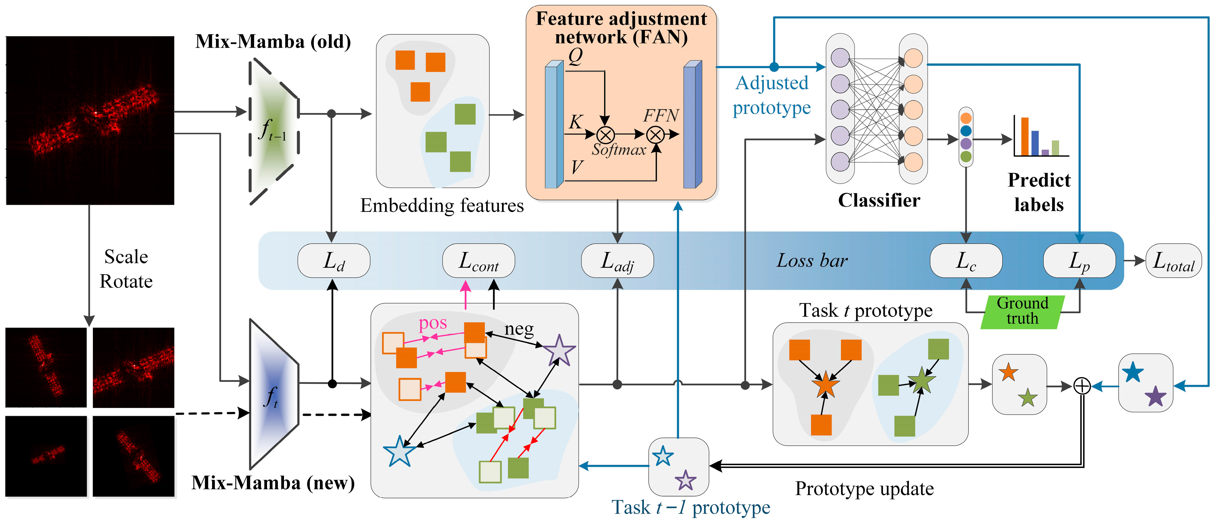
The overall structure of MMFAN is shown in
Figure 1, which can be divided into three parts: the Mix-Mamba backbone, FAN, and the loss bar. The Mix-Mamba backbone extracts the embedding features from the input samples and memorizes historical information by the prototypical vectors. FAN transfers the embedding features and prototypes between different tasks. The loss bar fuses five different loss functions to form a prototype-guided and non-exemplar incremental training procedure that guides the parameter updating of Mix-Mamba and FAN. In
Figure 1, the dotted and solid trapezoids represent the parameters of the Mix-Mamba backbone in task
t − 1 (old) and task
t (new), respectively. In the embedded feature zone, solid squares represent embeddings extracted by the original input images, slash squares represent embeddings extracted by the augmented input images, stars represent prototypes generated from embedded features, and pentagrams and squares with the same color correspond to the same target category. The blue arrows denote the generation and update flow of the prototypes, while the black arrows denote the data flow for network training.
Take task t as an example for generally describing the training and test of MMFAN. First, the parameters of Mix-Mamba in task t − 1 are fixed and copied as the old backbone (which does not involve gradient calculation) to serve as a reference for the historical memory. The new backbone participates in all gradient backpropagation and parameter updating and obtains classification results. Then, the input image is fed into both the old and new backbones to obtain the embedding features and , respectively. In order to constrain the new model from overfitting to the distribution of new classes, the distillation loss is calculated to minimize the difference between the features extracted by the old and new models, both from a new sample. For the new model, the augmented input samples (by scaling and rotating on ) are fed into the new backbone to obtain augmented features . Then and the historical prototypes serve as a contrastive learning template for supervised contrastive learning with , obtaining a contrastive loss .
FAN plays the role of transferring the feature distribution from the old backbone to the new backbone, i.e., . To achieve a better proximity between the adjusted features and the new backbone features, the feature adjustment loss is designed to minimize the difference between and . Another role of FAN is to adjust prototypes corresponding to all learned classes, thus mapping the old-class prototypes to the new feature space, i.e., . Then, the adjusted prototypes are input into the classifier to obtain the predicted prototype label, and the prototypical loss is computed by comparing the prototype label with the true class label. The features extracted by the new backbone are also fed into the classifier, and the classification loss is obtained by comparing them with the true class labels. Finally, the mean of corresponding to each class is computed to obtain the new class prototype for task t, which is then combined with to update the prototype library as .
2.3. Mix-Mamba
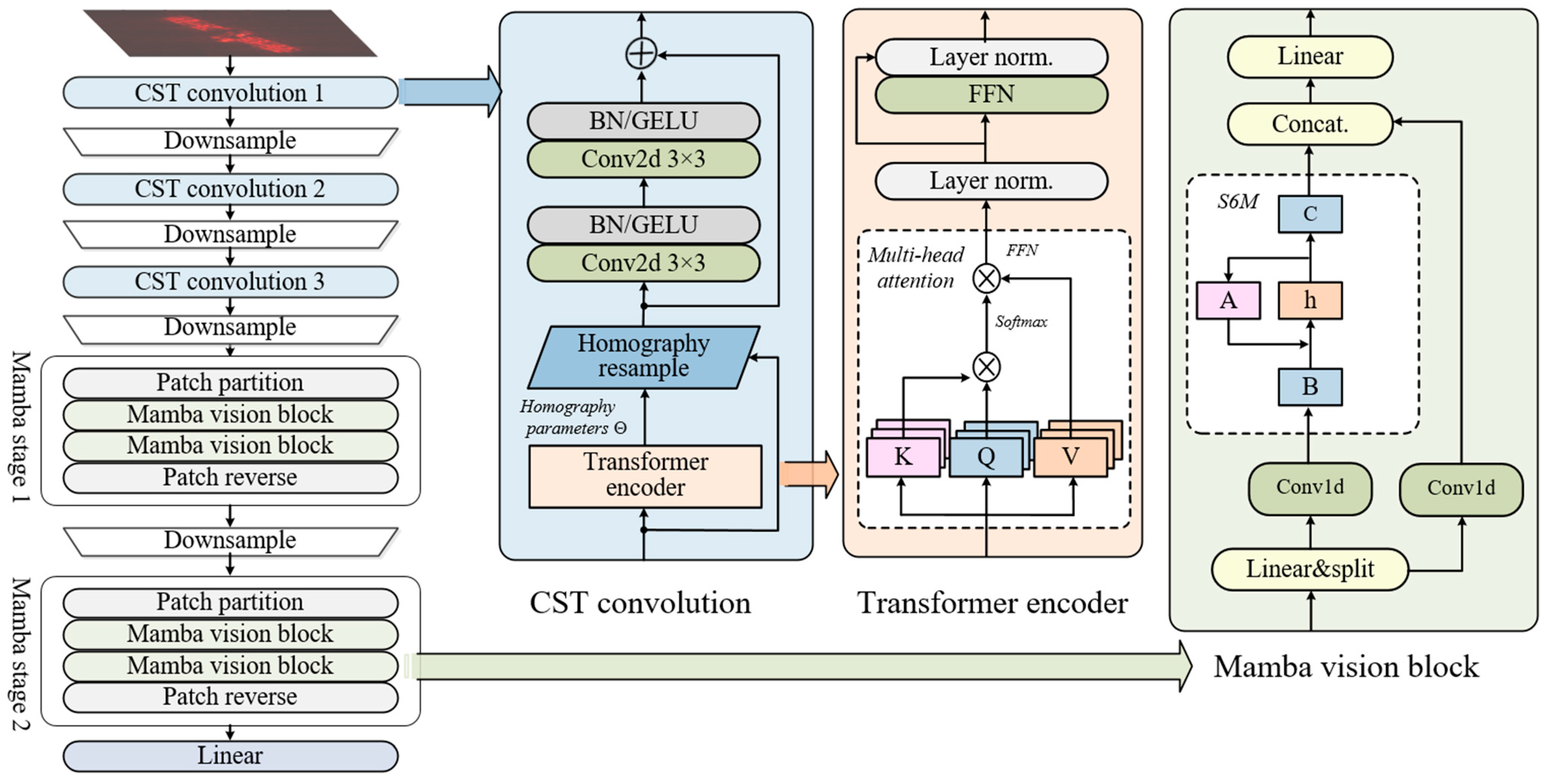
The network structure of Mix-Mamba is shown in
Figure 2, which is composed of three CST convolution stages and two Mamba stages. Compared with the original Mamba, Mix-Mamba mainly increases the CST convolution as a deformation-robust structure; in addition, motivated by Vision Transformer, Mix-Mamba uses the Mamba vision block to extract global features as 2D feature maps. As a backbone, Mix-Mamba takes image samples as input and obtains embedding vectors with the dimension of
. Due to the spatial inductive bias and strong local feature-extraction capabilities of convolutional networks, the CST convolution stages with residuals are designed to extract high-resolution features while adjusting deformations such as scaling, rotation, and perspective distortion in the feature maps. Mamba stages divide the feature maps into patches and employ selective scanning structured state-space models (S6M) [
59] for global context modeling, thus overcoming the limitations of capturing global spatial relationships for convolutional networks.
CST convolution stage: the CST operation illustrates three improvements over the original STN to figure out feature mismatch and shape mismatch: (1) introducing a more flexible homography transformation instead of the affine transformation [
60], (2) applying spatial transformations independently to multi-layer and each channel features, and (3) generating transformation parameters through a Transformer encoder rather than a simple linear function. By utilizing the cross-attention mechanism, the homography parameters are extracted from the image features through the learnable query vector. For the input feature map
, where
H and
W represent the height and width of the feature map and
C is the number of channels, the Transformer encoder calculates the attention scores by scaled dot-product attention. Let the attention value
V and key
K be obtained through linear mappings, while letting the query
Q be a learnable parameter for querying a preset length of output from the feature. We denote
as the hidden dimension of the Transformer encoder,
as a two-layer fully-connected network followed by the Gaussian error linear unit (GELU) non-linear activation function,
as the linear mapping from the feature dimension
to
, and
as the layer normalization, then the homography parameters
are obtained by
where the homography transformation parameters are extracted from the image features through the learnable query vector by using the Transformer cross-attention mechanism.
After obtaining
, it can be rearranged as
C groups of individual 3 × 3 transformation matrices according to the homogeneity, and then each channel of the feature maps can be resampled. The homography transformation can map the projections of 3D scatter points between different IPPs, thereby enabling the adjustment of the unknown deformation of ISAR images. Specifically, it calculates the pixel at position
in the output feature map
corresponding to the position
in the input feature map
, where
. Then, the output pixel value of the channel
c is obtained by bilinear interpolation as follows:
In each CST convolution stage, the adjusted feature map
is then fed into a two-layer 3 × 3 convolutional network (
) for local feature extraction, where each convolutional layer is followed by batch normalization (BN) and a GELU activation. Finally, the output of the CST convolution stage
is realized by element-wise adding the adjusted feature map for residual connecting, which is down-sampled by a 2 × 2 max-pooling (
) with doubled channel size, i.e.,
Mamba stage: The global feature extraction is realized by patch partition/reverse and two Mamba vision blocks [
61]. The feature map
is firstly partitioned (denoted by
) into
NC non-overlapping patches of size
, where
, and these patches are then flattened into vectors of length
, which is then linearly mapped and added with a learnable positional encoding
to obtain the patch embedding sequence
as
where
d denotes the feature dimension of this layer, and
denotes the process of patch partition.
In the Mamba vision block, the patch embedding sequence
is firstly linearly expanded along feature dimension from
d to 2
d, then it is split into two streams (denoted as
) with the same size: the Mamba flow
and the residual flow
, i.e.,
The Mamba flow consists of a 1D convolution with a kernel size of 3 (denoted as
), a sigmoid linear unit (
) activation, and an S6M operation (denoted as
). Conversely, the residual flow maintains the same structure without the S6M operation to preserve the local spatial relationships. Thereafter, the outputs of both streams are concatenated along the feature dimension (denoted as
) and linearly mapped back to the original dimension
d as
In order to recover the feature maps, the output of Mamba vision block
is obtained by linear mapping and patch reverse (denoted as
):
Finally, the feature downsampling and channel doubling are realized in the same way as (4). After the last Mamba stage, a global average pooling layer is designed to obtain the embedding feature vector corresponding to the input ISAR image.
In the Mamba vision block, S6M is the core for global feature extraction and contextual representation, which is improved from the SSM. The SSM handles long-term dependencies through sequence-to-sequence mappings and maintains a set of hidden state spaces to predict the output. For a 1D sequence
, where
and
is the sequence length, the continuous SSM defines the linear mapping from the input to the hidden state
and output
as
where
denotes a state transition matrix that governs the retention of the
,
denotes an input matrix that governs the update of
, and
denotes the output matrix that governs the contribution of the
to the output.
M is the dimension of the state space. Under the framework of deep learning, the continuous model is computationally inefficient and hard to train, so the SSM is discretized by converting the derivative into differences and aligning with the data sampling rate. The zero-order hold technique [
62] preserves the discrete data for a certain period and generates continuous output during that period. The preservation period is referred to as the sampling timescale
, and the discrete SSM takes the form of
where
To embed the discrete SSM into a deep network, the state updating can be expanded along the time dimension and implemented by a 1D convolution, i.e.,
where
is the convolution kernel. Therefore, the discrete SSM can be realized in parallel during training via convolution and al retain memory capability like a recurrent neural network (RNN). However, SSM is linear time-invariant, i.e.,
are static parameters, and their values do not directly depend on the input sequence. It limits the capability of long-term dependencies and global representations. Hence, S6M introduces selective scanning to grant the hidden states the ability to select content based on the input data. In the selective scanning, the step size
, the matrix
, and
are derived from the parallelized input sequence
as follows:
where
ensures that the timescale is positive, and
is the dimension of the selective scanning.
2.4. FAN
As a bridge between the distributions of old and new class features, FAN transfers the old-class prototypes to the feature space of the new tasks, thereby relieving catastrophic forgetting caused by prototype mismatch. Let the backbone network of task
t − 1 and task
t generate embedding features
and
, respectively, from the same sample of task
t, where
and
are the corresponding feature spaces formed by all possible features. To transfer the distribution of
to
with minimal cost, the optimal transportation model is established due to the discrete form of the Monge formula:
where
is the optimal transport function that minimizes the cost,
is the measure-preserving mapping of transporting from the feature space
to
, and
denotes the cost function transferring
to
; here, it can be represented as the Wasserstein distance between the features transferred by the old and new backbones, i.e.,
In order to realize end-to-end model training, the proposed FAN is also implemented by a Transformer encoder, as shown in (2), and the self-attention mechanism is applied here to obtain the internal relationship between old and new embedded features, thereby realizing the transfer of feature distribution. The parameter of FAN is optimized by the feature adjustment loss and prototype loss together.
2.5. Network Training
In the context of non-exemplar incremental learning, to alleviate the conflict between catastrophic forgetting and new-task learning, MMFAN combines feature replay and knowledge distillation techniques [
63]. The loss bar is proposed for prototype-guided and non-exemplar network training, where the supervised classification loss
, contrastive loss
, prototype loss
, unsupervised distillation loss
, and feature adjustment loss
are weighted and summed as follows:
where
are the weights for each loss.
Classification loss: It measures the accuracy of the class label predictions by the Mix-Mamba backbone and the linear classifier
, fulfilled by the following cross-entropy loss function:
where
K is the total number of classes, and
denotes the true class label.
Contrastive loss: It helps the backbone to compress the feature space and separate the different classes in incremental tasks. Since the historical data cannot be accessed, in the new feature space, the prototypes corresponding to old classes may be overlapped with the features extracted by the new backbone, increasing the error of decision boundaries. For a batch of input samples, the corresponding embedding features are noted as a set
, while the features of augmented samples are noted as a set
. The supervised contrastive loss takes
as a reference, with the features in
that share the same class as the reference are positive samples. In contrast, the prototypes in
and features in
longing to different classes of
are considered negative samples. Consequently, the inner product of features is employed to quantify the similarity between positive and negative samples thus:
where
and
are the labels corresponding to
and
,
denotes the number of the samples in
with the same class label as
, and
denote the temperature coefficient. In (18), the numerator encourages the features with the same class to come closer (reducing intra-class distance), while the denominator encourages pushing away the features with different classes (increasing inter-class distance). Therefore, the supervised contrastive loss prevents the dispersed feature distribution of new samples, thus mitigating the failure of historical decision boundaries and knowledge forgetting.
Prototype loss:
measures the precision of the classification result from the prototype
adjusted by FAN, which is realized by a cross-entropy function as
where
is the ground true of the prototype. Prototype loss ensures that the classifier enables discriminability for the adjusted old-class prototypes.
Distillation loss:
directly computes the L
2 distance between the embedding feature extracted by the old backbone
and the new backbone
, i.e.,
The distillation loss enables the new backbone to recover the historical knowledge.
Feature adjustment loss: As an unsupervised loss,
is designed to optimize FAN such that the prototypes can be mapped to an appropriate place in the new feature space, thus reducing the mismatch between the prototype and feature during cross-task incremental learning. Specifically,
calculates the L
2 distance between the adjusted feature
of the old backbone and the feature
of the new backbone, i.e.,


