Article

UIMM-Tracker: IMM-Based with Uncertainty Detection for Video Satellite Infrared Small-Target Tracking

Research Center for Space Optical Engineering, Harbin Institute of Technology, Harbin 150001, China
*
Author to whom correspondence should be addressed.
Remote Sens. 2025, 17(12), 2052; https://doi.org/10.3390/rs17122052
Submission received: 29 April 2025 / Revised: 10 June 2025 / Accepted: 11 June 2025 / Published: 14 June 2025

Abstract

Infrared video satellites have the characteristics of wide-area long-duration surveillance, enabling continuous operation day and night compared to visible light imaging methods. Therefore, they are widely used for continuous monitoring and tracking of important targets. However, energy attenuation caused by long-distance radiation transmission reduces imaging contrast and leads to the loss of edge contours and texture details, posing significant challenges to target tracking algorithm design. This paper proposes an infrared small-target tracking method, the UIMM-Tracker, based on the tracking-by-detection (TbD) paradigm. First, detection uncertainty is measured and injected into the multi-model observation noise, transferring the distribution knowledge of the detection process to the tracking process. Second, a dynamic modulation mechanism is introduced into the Markov transition process of multi-model fusion, enabling the tracking model to autonomously adapt to targets with varying maneuvering states. Additionally, detection uncertainty is incorporated into the data association method, and a distance cost matrix between trajectories and detections is constructed based on scale and energy invariance assumptions, improving tracking accuracy. Finally, the proposed method achieves average performance scores of 68.5%, 45.6%, 56.2%, and 0.41 in IDF1, MOTA, HOTA, and precision metrics, respectively, across 20 challenging sequences, outperforming classical methods and demonstrating its effectiveness.

1. Introduction

With the continuous development of new moving targets such as missiles, unmanned aerial vehicles (UAVs), and aircraft [1], the real-time tracking of targets to form continuous trajectories has become a primary requirement. Existing ground-based and air-based imaging methods can only operate within local spatio-temporal ranges [2], unable to meet the task requirements for long-duration continuous tracking. Space-based remote-sensing satellites, characterized by wide field of view and high timeliness, have emerged as the main direction for future moving target detection [3,4,5]. However, targets in remote-sensing images exhibit sparse characteristics [6], with most areas occupied by scene clutter. The targets share similar color and texture characteristics with cloud clutter and scene structural clutter [7], rendering visible light imaging unsuitable for target tracking tasks. Infrared imaging, compared to visible light, possesses powerful night imaging capabilities [8] and is widely used in characteristic measurement [9], disaster prediction [10], target detection [11], and target tracking [12] fields. Therefore, utilizing space-based infrared video satellites for tracking moving targets is a feasible technical approach, offering advantages such as sustainability, high robustness, and low interference. However, infrared small-target tracking still faces the following technical challenges: (1) Uncertainty in detection results: due to the complexity of space-based infrared scenes and the low energy and lack of morphological and textural features of small targets, there is a deviation between detection results and ground truth [13], introducing inherent errors caused by the detection algorithm that are difficult for tracking algorithms to eliminate (as shown in Figure 1a). (2) Trajectory interference: the spatial resolution of space-based infrared remote-sensing satellites is relatively low, causing targets and clutter that are close in spatial distance to couple, making it difficult to effectively distinguish target trajectories (as shown in Figure 1b). (3) Association difficulties: infrared small targets occupy only a few to tens of pixels in remote-sensing images, rendering traditional intersection over union (IoU) matching methods unsuitable for extremely small-scale targets (as shown in Figure 1c).
To address the aforementioned issues, numerous scholars have conducted corresponding research, the focus of which can be broadly classified into traditional methods [12] and deep-learning methods [14]. Traditional methods take detection results as input and combine data association algorithms to label targets with the same identity. These methods mainly include tracking based on target assignment (the Hungarian algorithm [15], linear assignment [16], and bipartite graph matching [17]), tracking based on probabilistic models (JPDA [18] and MHT [19]), tracking based on filters (the Kalman filter [20] and particle filter [21]), tracking based on graphical models (Bayesian estimation [22], random finite sets [23], minimum cost flow [24], and conditional random fields [25]), tracking based on trajectory modeling (global data association [26]), and tracking based on distributed frameworks (IMM [27]). Tracking based on target assignment has the advantages of low computational complexity and strong real-time performance, but its performance highly depends on the accuracy of the detector, and association errors are prone to occur in scenarios with target occlusion or a low signal-to-noise ratio. Tracking based on probabilistic models enhances tracking robustness through multi-hypothesis modeling but faces the problem of exponential growth in computational complexity, making it difficult to meet real-time requirements. Tracking based on filters effectively handles target motion uncertainty through state prediction but lacks adaptability to nonlinear/non-Gaussian noise. Tracking based on graphical models can achieve a global optimal association, but the modeling complexity is high, and parameter sensitivity is strong. Tracking based on trajectory modeling is suitable for dense target scenarios but requires a large amount of historical trajectory data for support. Tracking based on distributed frameworks addresses target maneuverability through multi-model interaction but has a strong dependence on prior motion models.
Traditional methods primarily address three components: target feature extraction, state prediction, and data association. Feature extraction aims to leverage the morphological and structural uniqueness of targets to extract their appearance features, which need to differentiate from other targets’ features and remain temporally invariant. For example, Wang et al. filter low-quality feature embeddings through a trajectory selection strategy and transition feature states based on an adaptive exponential moving average method [28]. State prediction utilizes the motion characteristics of targets to construct a state transition model, enabling the acquisition of target states such as position and velocity at future time steps. State prediction can be used in conjunction with appearance information, such as in optical flow methods [29], or independently, such as using LSTM to mine historical information to predict the current state [30]. In recent years, some novel state prediction methods have emerged, such as utilizing the Mamba architecture to predict target positions [31]. Data association algorithms address the matching problem between trajectories and detections, primarily implemented through cost computation based on appearance [32] or motion [33] features, combined with classical methods like the Hungarian algorithm for target association. Appearance and motion features are obtained during the feature extraction phase. Deep-learning methods rely heavily on extensive data annotation. Currently, remote-sensing satellite infrared small-target tracking datasets are limited, and factors such as satellite orbit, attitude, and payload design parameters directly impact image quality, making it challenging to adapt training to all scenarios.
Traditional methods and deep-learning approaches exhibit distinct advantages and limitations in space-based infrared small-target tracking. Due to the long imaging distances inherent to space-based systems, moving targets manifest as small-scale objects with weak radiation signatures on focal plane arrays. Deep-learning methods typically require learning target appearance features for inter-frame data association. However, the non-unique appearance characteristics of dim, small infrared targets combined with spatial downsampling and pooling operations during feature extraction may discard critical target details, leading to feature extraction failures and subsequent erroneous associations. Moreover, the scarcity of existing space-based infrared small-target tracking datasets imposes significant constraints on deep-learning approaches, which depend heavily on extensive annotated data. Under limited training samples, these algorithms demonstrate restricted generalization capabilities when confronted with complex operational scenarios. In contrast, traditional methods employ predefined prior constraints to govern target prediction and association processes, effectively circumventing global error propagation while remaining applicable to data-scarce environments. Nevertheless, current conventional approaches neglect the critical influence of detection uncertainty, which directly impacts measurement accuracy in observation models and consequently affects target state updates. The unaccounted measurement errors ultimately degrade both association reliability and localization precision.
To address the aforementioned issues and meet the requirements of infrared remote-sensing sparse-data small-target tracking applications, we propose the UIMM-Tracker based on the accuracy of state estimation for complex maneuvering targets within the IMM framework. This method obtains target uncertainty measurements during the non-maximum suppression processing stage of detection results. Unlike the classical IMM method, it utilizes these uncertainty measurements in the target state update and data association processes, transferring the detector’s empirical distribution into the tracking process to enhance tracking accuracy. Moreover, to address the mismatch of the given prior Markov transition matrix for target state switching in traditional IMM methods, we specifically design a dynamic Markov transition matrix construction method. This method updates model transition probabilities by combining historical dynamic information and current static information. Finally, in the data association phase, we leverage the advantages of intersection over union (IoU) and normalized Wasserstein distance (NWD) to associate targets of different scales, transferring uncertainty into the cost calculation process. To address the ambiguity attributes of the cost matrix caused by uncertain values, we take classical scale invariance and energy invariance assumptions as examples to handle ambiguously matched tracks and targets, verifying the importance of measuring detection uncertainty distribution and the necessity of disambiguating the cost matrix, thereby achieving high-precision target tracking.
Overall, the main contributions of the paper are as follows:
(1) Addressing the challenge of eliminating tracking errors, we inject detection uncertainty measurements into the observation noise of the IMM, which is used to propagate the empirical distribution of the detector during the observation prediction and state update processes, thereby obtaining more accurate state estimation results.
(2) A dynamically adaptive Markov transition matrix is proposed, enabling the IMM framework to adjust current model mixing weights based on the current likelihood probabilities of the models and the rate of change in model probabilities. This achieves precise matching between the target’s motion state and motion models, solving the problem of target trajectory crosstalk.
(3) To address the challenge of associating tracks with detection results in remote-sensing infrared images, this paper incorporates detection uncertainty measurements into the cost calculation process of data association. Using scale and energy invariance assumptions as examples, further constraints are applied to ambiguous matches between tracks and detections, thereby reducing incorrect associations.

2. Related Works

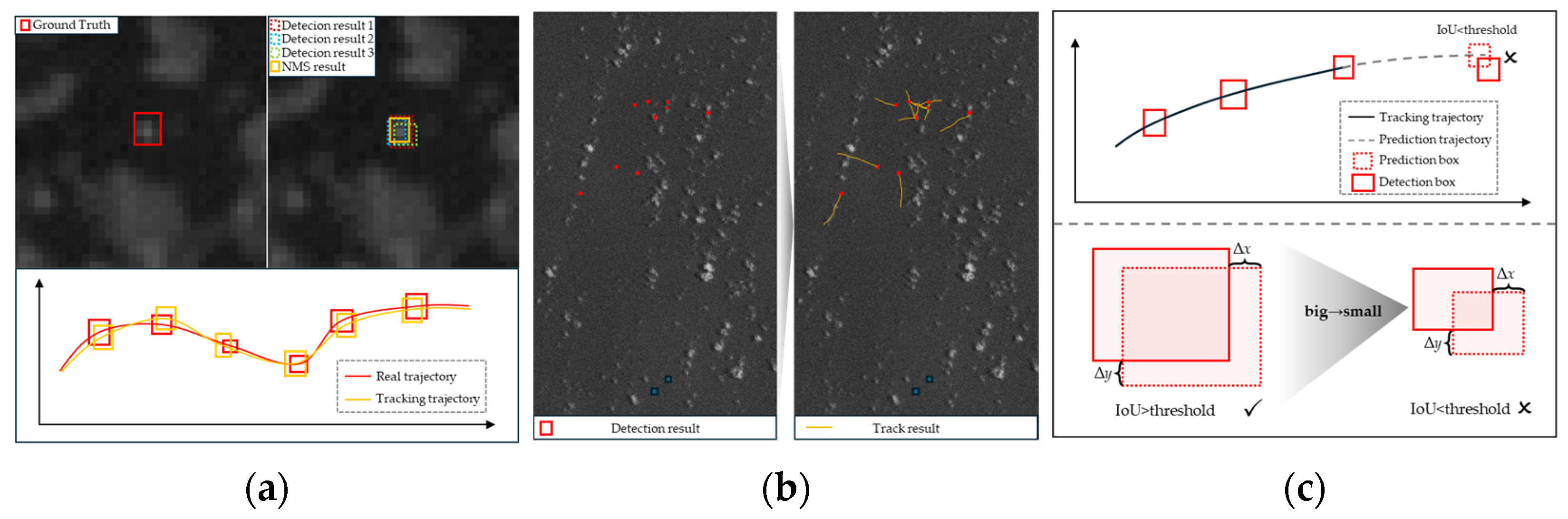
2.1. Small-Target Tracking in Video Satellites

Small-target tracking in video satellites is a pivotal technology in the field of remote sensing, aimed at continuously locating and associating targets (such as aircraft, ships, etc.) that are small in size (typically less than 0.1% of the image area), have low signal-to-noise ratios, and exhibit complex motion patterns from satellite video sequences. It primarily addresses issues such as the lack of apparent target features due to resolution limitations, strong background interference (e.g., clouds, surface textures), and nonlinear motion (rapid movement of targets from a satellite’s perspective). Most existing methods embed strategies, modules, or mechanisms within the classic multi-target tracking framework to address the inherent challenges of small-target tracking applications in remote sensing, thereby meeting practical application requirements. Specific improvements are categorized into three types: enhanced traditional approaches, domain-adaptive deep-learning methods, and hybrid intelligent frameworks. In enhanced traditional approaches, Hua et al. [34] introduced a perspective-aware UKF that models target motion using angular measurements rather than target coordinates in the image plane, thereby reducing drift errors during long-term tracking. In domain-adaptive deep-learning methods, HB-YOLO [35] employs an improved HorNet to replace conventional convolutions for higher-order spatial interactions and replaces ELANs with the BoTNet attention mechanism to enhance small-target features. MCTracker [36] combines inter-frame motion correlation with multi-scale cascaded feature enhancement to improve the feature fusion representation capabilities of multiple modules. To address the issue of data annotation, scholars have also used frameworks similar to MetaEarth [37] to generate synthetic satellite videos with physics-based noise models (e.g., atmospheric turbulence and jitter effects) for pretraining. In hybrid intelligent frameworks, Revach et al. [38] embedded a structured linear Gaussian state-space model and a dedicated recurrent neural network module into the Kalman filter’s process, enabling the model to learn from data to achieve target state estimation in nonlinear environments with low complexity.
However, the aforementioned methods lack a description of uncertainty in target detection results, making it impossible to further guide the generation of high-precision tracking results. Additionally, corresponding solutions are absent for issues such as target trajectory crosstalk and variable-scale association. Based on the shortcomings of existing methods, this paper proposes the UIMM-Tracker framework for small-target tracking in infrared remote-sensing satellite imagery.

2.2. Infrared Small-Target Tracking

To address the challenges posed by the small size, low signal-to-noise ratio (SNR), weak texture features, and frequent interference from complex backgrounds in infrared small-target tracking, researchers have proposed various approaches, including traditional methods and deep-learning-based techniques. Early infrared small-target tracking primarily relied on classical filtering methods, such as Kalman filtering and particle filtering. These methods achieve target state prediction and update by constructing motion and observation models. However, their performance degrades when dealing with complex background interference or target occlusion. For instance, [39] introduced an improved particle filtering algorithm that enhances robustness to target motion to some extent but still exhibits limitations in dynamic scenarios. In recent years, the rapid development of deep-learning techniques has provided new solutions for infrared small-target tracking. Shan et al. [40] proposed the OSTrack model [41], based on a single-stream deep-learning framework, which integrates feature extraction and target tracking processes, significantly improving the accuracy and robustness of infrared small-target tracking. By analyzing the motion characteristics of infrared small targets, [42] designed the IRSDT framework, which combines deep learning with traditional methods to enhance tracking performance under complex backgrounds. Siamese networks [43] are classical methods in target tracking. Considering the weak texture and small size of infrared small targets, Qian et al. [44] proposed the SiamIST algorithm, which improves the SiamRPN network structure to enhance precise localization of small targets during tracking. To alleviate the issue of insufficient data, data augmentation techniques are widely applied. Zhang et al. [45] utilized generative adversarial networks (GANs) to generate synthetic infrared small-target data, effectively expanding the training dataset. Additionally, the fusion of multimodal data has become a research hotspot. For example, [46] proposed a joint tracking framework that integrates infrared and visible light information, significantly enhancing the robustness of tracking algorithms.
This paper addresses the weak and small characteristics of remote-sensing infrared targets and their complex maneuvering states by designing the UIMM-Tracker, which integrates detection uncertainty measurement, IMM, a dynamic Markov transition matrix, and uncertainty-based association cost calculation, enabling precise tracking and high-accuracy localization of targets.

2.3. Application of Uncertainty Measurement

Uncertainty has been widely applied across various fields. For example, in autonomous driving, uncertainty is used to adjust decision-making strategies, preventing accidents caused by incorrect detections [47]. In object detection, uncertainty information can dynamically adjust the confidence threshold of detectors, reducing false positives and missed detections, and adapting to different application scenarios [48]. During data annotation, uncertainty helps select the most informative samples for labeling, reducing annotation costs and improving model performance [49]. In model evaluation and improvement, analyzing uncertainty distribution can reveal weaknesses in specific scenarios or categories, guiding data augmentation or model optimization [50]. In human–machine collaboration scenarios, such as medical image analysis or security monitoring, uncertainty serves as a cue to help human experts focus on high-risk areas or detection results [51]. On resource-constrained edge devices, uncertainty information can dynamically adjust computation paths, such as skipping high-confidence detection boxes and allocating resources to process high-uncertainty regions [52]. In anomaly detection and scene understanding, uncertainty analysis enables the detection of anomalous objects or unfamiliar scenes, enhancing the model’s adaptability to unknown environments [53]. This paper introduces detection uncertainty into the task of remote-sensing infrared small-target tracking, improving target matching accuracy and reducing tracking drift.

3. Method

In this section, we provide a detailed explanation of the components and implementation principles of the proposed UIMM-Tracker. Section 3.1 introduces the overall framework of the tracker, while Section 3.2,Section 3.3,Section 3.4 and Section 3.5 describe the complete process, from detection uncertainty measurement to the tracker’s output at a single time step. Section 3.6 explains the construction method of the dynamic Markov transition matrix, which serves as input for target state estimation in the next time step. Section 3.7 introduces the trajectory completion method, which is used to restore missing target information.

3.1. Overview

The overall framework of the UIMM-Tracker is shown in Figure 2. The tracker consists of four steps: uncertainty measurement of detection results, state prediction (input interaction and filtering), data association, and model update and data fusion. The results of uncertainty measurement serve as inputs for data association and model state updates, transferring the detector’s uncertainty empirical distribution into the target tracking process. Finally, the Markov transition probability matrix is dynamically adjusted by combining current and historical information, enabling the model to adapt to complex target motion states. The overall workflow of the algorithm is shown in Algorithm 1.
Algorithm 1 UIMM-Tracker execution process
  Input: Image sequence 1~ n, Detection result d = [ x n , y n , w n , h n , s n ] n = 1 N , Detection uncertainty covariance R 0 = diag ( σ x 2 , σ y 2 , σ w 2 , σ h 2 ) 0
  Output: Trajectory T , The mean of the updated x ^ k | k j , updated state covariance p ^ k | k j , fused state mean x k , fused state covariance p k , Markov transition matrix M k , model probability u k
  Initial: CT model control variable y 1 y t = [ a x , a y , ω ˙ ] T , Markov transition matrix M 0 = 0.8 , 0.1 , 0.1 ; 0.1 , 0.8 , 0.8 ; 0.1 , 0.1 , 0.8 , model probability u 0 = 1 , 0 , 0 ; 0 , 1 , 0 ; 0 , 0 , 1 , target initial state mean x ^ 0 | 0 1 ~ x ^ 0 | 0 N , Initial state covariance p ^ 0 | 0 1 ~ p ^ 0 | 0 N = diag ( R 0 , 0.3 , 0.3 , 3 ) .
1   for k in 1~t do
2 Uncertainty of Measurement Detection Result d:  R k = diag ( σ x 2 , σ y 2 , σ w 2 , σ h 2 ) k ;
3  Input Interaction and Filtering;
4    Calculate the mixed state mean x ^ k 1 | k 1 o j and mixed covariance p ^ k 1 | k 1 o j for model j based on the updated state mean x ^ k 1 | k 1 i | i = 1 N and updated state covariance p ^ k 1 | k 1 i | i = 1 N of all models;                                         #(1)~(4)
5    Obtain the sigma points of the UKF based on x ^ k 1 | k 1 o j and p ^ k 1 | k 1 o j ;                               #(5)
6    Obtain the predicted mean x ^ k | k 1 o j and predicted covariance p ^ k | k 1 o j ;                                  #(6)~(8)
7    Calculate the observation predicted mean z ^ k | k 1 o j and observation predicted covariance s ^ k | k 1 o j ;                 #(9)~(11)
8  Data Association;
9    Combine NWD and IoU distance to calculate the cost C p q of trajectory T p and detection d q ;                 #(12)~(15)
10    Iterate over p and q to obtain the cost matrix C = { C p q } p = 1 , q = 1 p = P , q = Q ;
11    Calculate the scale cost U p q s s for ambiguous matches of trajectory T p and detection d q s ;                      #(16)
12    Calculate the scale cost U p q s e for ambiguous matches of trajectory T p and detection d q s ;                   #(17)~(18)
13    Combine the scale cost and energy cost to obtain the additional cost matrix U;                        #(19)
14    Integrate the cost matrix and apply Hungarian matching to obtain the association result Ƶ k | k 1 o j ;
15  Model Probability Update;
16    Calculate the cross-covariance C o v k | k 1 j between the predicted mean x ^ k | k 1 o j and the association result Ƶ k | k 1 o j ;            #(20)
17    Calculate the Kalman gain K k j ;                                              #(21)
18    Calculate the updated state mean x ^ k | k j and updated state covariance p ^ k | k j ;                         #(22)~(23)
19  Data Fusion;
20    Calculate the likelihood probability Λ k j using Ƶ k | k 1 o j , z ^ k | k 1 o j and s ^ k | k 1 o j ;                              #(24)
21    Calculate the model probability u k j using Λ k j , Markov transition probability M k 1 i j , and the model probability u k 1 i ;        #(25)
22    Calculate the fused state mean x k and fused covariance p k using u k j , x ^ k | k j , and p ^ k | k j ;                  #(26)~(27)
23  Dynamic Markov Transition Matrix;
24    Calculate the state prediction error e p ˜ k j using the observation predicted mean z ^ k | k 1 o j and the association result Ƶ k | k 1 o j ;
25    Calculate the normalized likelihood probability Λ ˜ k j ;
26    Calculate the rate of change of model probability ρ k j ;
27    Calculate the Markov transition probability matrix M k ;                             #(28)~(29)
28  Filling Discontinuous Trajectories;
29    For discontinuous trajectories from time t1 to t2, use the fused state mean x t 2 at time t2 and the predicted mean x ^ t 2 | t 2 1 to correct the prediction error.                                                     #(30)
30  end

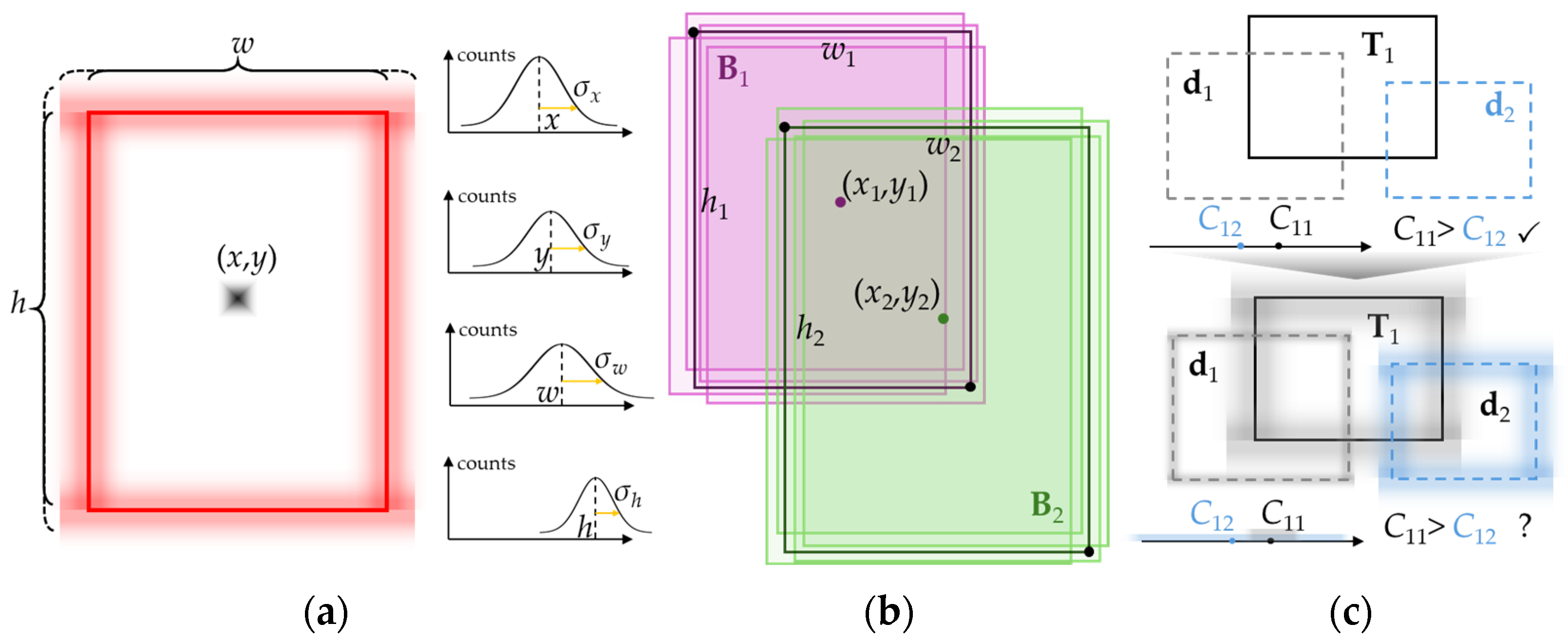
3.2. Uncertainty Measurement of Detection Results

The results of object detection consist of a series of bounding boxes and confidence scores. For a given object, the detection result is described as ( x n , y n , w n , h n , s n ) , where n = 1 , 2 , , N and N represent the number of detection boxes. ( x n , y n ) denotes the center position of the n-th detection box, ( w n , h n ) represents its width and height, and s n [ 0 , 1 ] is the confidence score of the n-th detection box. After applying non-maximum suppression (NMS), the optimal bounding box is retained. In conventional tracking methods, the de-redundant bounding box is used as input to the tracking algorithm, and association methods are employed to link bounding boxes belonging to the same object, ultimately producing the tracking results. This process treats redundant detection results as irrelevant information and models the observation noise at time step k as a random distribution with a mean of 0 and a root mean square of R k , making it difficult to eliminate detection biases during the tracking process.
We model the detection results as a spatial distribution with a standard deviation σ. σ is calculated by measuring the variance of each detection result relative to the bounding box retained after non-maximum suppression (NMS) and is propagated to the tracker to quantify the observation noise of the IMM tracker, thereby characterizing the distribution range of the observations. As shown in Figure 3a, the modeled R k = diag ( σ x 2 , σ y 2 , σ w 2 , σ h 2 ) k k = 1 N , where diag ( ) represents a diagonal matrix.

3.3. Input Interaction and Filtering

The target state mean of the IMM filter output at time step k is defined as x k = [ x k , y k , w k , h k ] T . Considering the CV model, CA model, and CT model, the target state space is represented as [ x k , y k , w k , h k , x ˙ k , y ˙ k , θ k ] T , where θ k denotes the target’s rotation angle at time step k.
The conditional probability matrix of model transitions is defined as Π = { π i j } i , j = 1 N , where π i j = P ( M k j M k 1 i ) represents the probability of transitioning from model i to model j. M t denotes different motion models, with t = 1 , 2 , N , where N is the number of models. The x ^ k 1 | k 1 i and p ^ k 1 | k 1 i represent the updated state mean and updated covariance output by model i at time k − 1, respectively. The mixed initial state and corresponding covariance are calculated based on the model transition probability Π :
x ^ k 1 | k 1 o j = i = 1 N π i j x ^ k 1 | k 1 i
p ^ k 1 | k 1 o j = i = 1 N π i j p ^ k 1 | k 1 i + ( x ^ k 1 | k 1 o j x ^ k 1 | k 1 i ) ( x ^ k 1 | k 1 o j x ^ k 1 | k 1 i ) T
where x ^ k 1 | k 1 o j and p ^ k 1 | k 1 o j represent the mixed initial state variable and mixed initial covariance of the j-th model after mixing, respectively. The calculation of π i j is as follows:
π i j = 1 ς ¯ j M k 1 i j u k 1 i
ς ¯ j = i = 1 N M k 1 i j u k 1 i
where M k 1 i j represents the Markov transition probability from model i to model j at time k − 1, and u k 1 i denotes the probability of model i at time k − 1. The calculation of ς ¯ j is for normalization. M k 1 i j adapts based on the target state to fit the motion model, enabling accurate tracking of complex maneuvering targets. The detailed design process is described in Section 3.6.
For each model j, the UKF is used for state prediction. The UKF predicts the distribution of data by propagating sigma points through nonlinear transformations, replacing the complex linearization process. The sigma points are sampled as follows:
𝒳 k 1 o j = x ^ k 1 | k 1 o j ± ( n + λ ) p ^ k 1 | k 1 o j
where 𝒳 k 1 o j represents the sigma point matrix, n denotes the dimension of the state, and λ is a parameter of the UKF, defined as λ = α 2 ( n + κ ) n , where α is the scaling parameter and κ is set to 3 − n.
Each sigma point is propagated through the state transition function f j ( · ) for state prediction:
𝒳 k | k 1 o j = f j ( 𝒳 k 1 o j )
The predicted state mean x ^ k | k 1 o j and the predicted covariance p ^ k | k 1 o j are obtained as follows:
x ^ k | k 1 o j = q = 1 2 n + 1 W q ( m ) 𝒳 k | k 1 , q o j
p ^ k | k 1 o j = q = 1 2 n + 1 W q ( c ) ( 𝒳 k | k 1 , q o j x ^ k | k 1 o j ) ( 𝒳 k | k 1 , q o j x ^ k | k 1 o j ) T + Q j
where W q ( m ) and W q ( c ) represent the weights for the calculation of the state mean and covariance in the UKF process, respectively.
The sigma points after state prediction are propagated as follows through the observation function h ( ) :
γ k | k 1 o j = h ( 𝒳 k | k 1 o j )
The measurement prediction mean z ^ k | k 1 o j is used for subsequent data association, which is described in Section 3.4:
z ^ k | k 1 o j = q = 1 2 n + 1 W q ( m ) ( γ k | k 1 , q o j )
The measurement prediction covariance s ^ k | k 1 o j is used in the likelihood probability calculation process described in Section 3.5. The specific calculation is as follows:
s ^ k | k 1 o j = q = 1 2 n + 1 W q ( c ) ( γ k | k 1 , q o j z ^ k | k 1 o j ) ( γ k | k 1 , q o j z ^ k | k 1 o j ) T + R k
where Rk represents the covariance of the detection results at time k, obtained in Section 3.2.

3.4. Data Association

To account for the association cost calculation of targets with different scales, inspired by [54], we adopt a scale-aware joint NWD-IOU distance to get the cost Cpq between the trajectory T p (derived from the measurement prediction mean z ^ k | k 1 o j ) and the detection d q as follows:
C p q = 1 1 + e ( A / C 1 ) × IoU + ( 1 1 1 + e ( A / C 1 ) ) × NWD ( C )
where A is the area enclosed by the detection box d q , and C is a constant balancing the IoU and NWD distances.
Due to the uncertainty of detection results, the IoU and NWD costs of T p and d q are extended from a single value to a range. The corresponding cost C p q = C ¯ p q ± Δ C p q , according to Equation (11), is calculated as follows:
Δ C p q = 1 1 + e ( A / C 1 ) × Δ IoU + ( 1 1 1 + e ( A / C 1 ) ) × Δ NWD ( C )
Since the area fluctuation range of small-scale targets is limited to the pixel level, its impact on the above equation is negligible. A can thus be treated as a constant, which is calculated after applying NMS to the detection results. Therefore, the factors ultimately affecting the cost range are Δ IoU and Δ NWD . In the estimation of Δ IoU , the calculation of IoU is more sensitive to the uncertainty in the intersection region. Thus, Δ IoU is represented by the uncertainty of the intersection region, i.e., Δ IoU / IoU = Δ A / A , as shown in Figure 3b. For bounding boxes B 1 = ( x 1 , y 1 , h 1 , w 1 ) and B 2 = ( x 2 , y 2 , h 2 , w 2 ) with inaccuracies Δ B 1 = ( Δ x 1 , Δ y 1 , Δ h 1 , Δ w 1 ) and Δ B 2 = ( Δ x 2 , Δ y 2 , Δ h 2 , Δ w 2 ) , respectively, the relationship between Δ IoU and IoU is derived based on the principle of linear error propagation as follows:
Δ IoU IoU ¯ = Δ A A = Δ x 2 Δ x 1 + 1 2 ( Δ w 2 + Δ w 1 ) x 2 x 1 + 1 2 ( w 2 + w 1 ) + Δ y 2 Δ y 1 + 1 2 ( Δ h 2 + Δ h 1 ) y 2 y 1 + 1 2 ( h 2 + h 1 )
The uncertainty Δ r , r { x 1 , y 1 , w 1 , h 1 , x 2 , y 2 , w 2 , h 2 } , represents the standard deviation of the corresponding measurement, which is obtained in Section 3.2 by measuring the standard deviation of each detection result. Based on the above calculations, the range of IoU values is IoU ¯ p q ± Δ IoU p q .
In the calculation of Δ NWD , since the computation of the center point Wasserstein distance d c and the scale Wasserstein distance d s are nonlinear processes, we simplify the operation by using a first-order Taylor expansion to approximate the derivative process and neglect higher-order terms. The relationship between Δ NWD and NWD is derived as follows:
Δ NWD NWD ¯ = Δ d c + Δ d s d c + d s ( w 1 Δ h 1 + h 1 Δ w 1 + w 2 Δ h 2 + h 2 Δ w 2 ) 2 ( w 1 h 1 + w 2 h 2 ) Δ d c = ( x 2 x 1 ) ( Δ x 2 Δ x 1 ) + ( y 2 y 1 ) ( Δ y 2 Δ y 1 ) d c Δ d s = ( w 2 w 1 ) ( Δ w 2 Δ w 1 ) + ( h 2 h 1 ) ( Δ h 2 Δ h 1 ) 2 d s d c = ( x 2 x 1 ) 2 + ( y 2 y 1 ) 2 d s = ( ( w 2 w 1 ) / 2 ) 2 + ( ( h 2 h 1 ) / 2 ) 2
The uncertainty Δ r , r { x 1 , y 1 , w 1 , h 1 , x 2 , y 2 , w 2 , h 2 } , is obtained in the same manner as in the Δ IoU calculation process. Based on the above calculations, the range of NWD values is NWD ¯ p q ± Δ NWD p q . Finally, the cost range between trajectory T p and detection d q is C p q [ C ¯ p q Δ C p q , C ¯ p q + Δ C p q ] .
In the association process, the cost matrix C = { C p q } p = 1 , q = 1 p = P , q = Q is solved to obtain the optimal assignment between trajectories and detections, where P represents the number of trajectories at the current time step, and Q represents the number of detections. However, with the introduction of uncertain measurements, each element in the cost matrix expands from a single value to an interval range, disrupting the one-to-one matching relationship between trajectories and detections (as shown in Figure 3c) and introducing ambiguous matching cases. To correctly associate trajectories with detections d q , an additional cost matrix U = { U p q s } q s = 1 q s = Q s (where Qs represents the number of ambiguously matched detections) is introduced to replace the ambiguous elements in the original cost matrix C. Finally, the Hungarian algorithm is applied to obtain the association results between trajectories and detections.
We introduce the following two classic, simple prior assumptions of space-based infrared small-target imaging to design the additional cost matrix U:
(1) The target’s scale remains nearly consistent across consecutive frames, meaning targets with significant scale differences should have lower matching degrees;
(2) The target’s energy remains nearly consistent across consecutive frames, meaning targets with significant energy differences should have lower matching degrees.
Based on the above two assumptions, U consists of two components: the shape constraint matrix U s and the energy constraint matrix U e . The calculation of U s is as follows:
A T ˜ p = ( A T p A T ¯ ) / σ T A d ˜ q s = ( A d q s A d ¯ ) / σ d U p q s s = e 1 2 ( A T ˜ p A d ˜ q s ) 2
where A T p , A T ¯ , and σ T represent the bounding box area of trajectory p, the mean area of the trajectory, and the standard deviation of the trajectory area, respectively. Thus, A T ˜ p is the normalized bounding box area with a mean of 0 and a standard deviation of 1. Similarly, A d ˜ q s is the normalized result for the ambiguously matched detection. U p q s s is the distance metric function between the two, normalized to [0, 1], where a closer match between them results in U p q s s approaching 1.
The calculation of U e differs slightly from that of U s . In infrared scenarios, targets may move across different backgrounds, and the energy of a target point can be considered as the sum of the target energy and the background energy. Therefore, directly using the grayscale value of the target point for calculation introduces background interference. To address this issue, we use the signal-to-clutter ratio (SCR) to eliminate the influence of background energy. For detection d q s , the grayscale value of the target point is E q s , the mean background grayscale is B ¯ q s , and the background standard deviation is σ q s B . The signal-to-clutter ratio S C R q s is calculated as follows:
S d q s = E q s B ¯ q s σ q s B
The calculation of U e is as follows:
S T ˜ p = ( S T p S T ¯ ) / σ S T S d ˜ q s = ( S d q s S d ¯ ) / σ S d U p q s e = e 1 2 ( S T ˜ p S d ˜ q s ) 2
where S T p , S T ¯ , and σ S T represent the SCR of trajectory p, the mean SCR of the trajectory, and the standard deviation of the trajectory SCR, respectively. The resulting S T ˜ p is the normalized SCR of trajectory p. Similarly, S d ˜ q s is the normalized SCR of detection qs. U p q s e measures the distance between the two and is normalized to [0, 1]. Therefore, the additional cost matrix U is
U p q s = λ U p q s s + ( 1 λ ) U p q s e
where λ is the coefficient used to balance the shape constraint and energy constraint.
During the matching process between the measurement prediction z ^ k | k 1 o j of the IMM and the detections, the association results generated by each model are defined as Ƶ k | k 1 o j and are used for subsequent model state updates.

3.5. Model Probability Update and Data Fusion

Using the predicted sigma points 𝒳 k | k 1 o j (Equation (6)), the predicted state mean x ^ k | k 1 o j (Equation (7)), the associated detection results Ƶ k | k 1 o j , and the measurement prediction mean z ^ k | k 1 o j (Equation (10)), the cross-covariance matrix between x ^ k | k 1 o j and Ƶ k | k 1 o j is calculated as follows:
C o v k | k 1 j = q = 1 2 n + 1 W q ( c ) ( 𝒳 k | k 1 o j x ^ k | k 1 o j ) ( Ƶ k | k 1 o j z ^ k | k 1 o j ) T
The Kalman gain is calculated using the cross-covariance matrix and the observation covariance. According to Section 3.2, the observation covariance R k of the measurement is obtained. Therefore, the Kalman gain K k j is
K k j = C o v k | k 1 j ( R k ) 1
The updated state mean and covariance are
x ^ k | k j = x ^ k | k 1 o j + K k j ( Ƶ k | k 1 o j z ^ k | k 1 o j )
p ^ k | k j = p ^ k | k 1 o j K k j R k ( K k j ) T
After obtaining the updated state x ^ k | k j and updated covariance p ^ k | k j for each model, they are used as inputs for the IMM tracking algorithm in the next time step. Simultaneously, the associated detection results Ƶ k | k 1 o j is used to calculate the likelihood probability of each model, which represents the degree of matching between the model’s measurement prediction mean and the actual observation. The model likelihood probability is calculated based on Bayesian theory, and the specific calculation is as follows:
Λ k j = P ( z k M k j ) = 1 | 2 π s ^ k | k 1 o j | exp 1 2 ( Ƶ k | k 1 o j z ^ k | k 1 o j ) T ( s ^ k | k 1 o j ) 1 ( Ƶ k | k 1 o j z ^ k | k 1 o j )
where s ^ k | k 1 o j represents the measurement prediction covariance (Equation (11)), and z ^ k | k 1 o j denotes the measurement prediction mean (Equation (10)).
The probability u k j of model j is calculated by combining the likelihood probability Λ k j and the Markov transition probability M k 1 i j . The calculation is as follows:
u k j = Λ k j i = 1 N M k 1 i j u k 1 i j = 1 N ( Λ k j i = 1 N M k 1 i j u k 1 i )
Based on u k j , combined with the updated state mean results x ^ k | k j and updated covariance p ^ k | k j of all models, the IMM fused output for the fused target state mean and fused covariance is
x k = j = 1 N u k j x ^ k | k j
p k = j = 1 N u k j p ^ k | k j + ( x ^ k | k j x k ) ( x ^ k | k j x k ) T

3.6. Dynamic Markov Transition Matrix

The fused target state is directly influenced by the Markov transition matrix M k 1 i j , which is predefined in traditional IMM methods. However, for complex maneuvering targets, the predefined matrix cannot adapt to the rapid switching of motion models required for frequent state transitions. Therefore, we design a dynamic Markov transition matrix that autonomously updates by comprehensively considering model prediction errors, likelihood probability calculations, and the changes in model probabilities over two consecutive time steps. This approach improves the accuracy of the IMM algorithm.
Specifically, the normalized state prediction error of model j at time k − 1 is e p ˜ k j = z ^ k | k 1 o j Ƶ k | k 1 o j / j = 1 N z ^ k | k 1 o j Ƶ k | k 1 o j , the normalized likelihood probability at time k is Λ ˜ k j = Λ k j / j = 1 N Λ k j , and the model probabilities at times k − 1 and k are u k 1 j and u k j , respectively. The rate of change in model probability at time k is denoted as ρ k j = exp ( u k j u k 1 j ) . e p ˜ k j [ 0 , 1 ] , where a smaller e p ˜ k j indicates that the predicted measurement z ^ k | k 1 o j is closer to the detected measurement Ƶ k | k 1 o j , suggesting a higher degree of consistency between the model and the actual situation, and thus the model transition probability should be higher. Λ ˜ k j [ 0 , 1 ] , where a larger Λ ˜ k j indicates a higher likelihood probability for model j, thus the model transition probability should also be higher. ρ k j [ 1 / e , e ] , representing the change in the model’s ability to match the actual motion over two consecutive time steps, ρ k j > 1 indicates an increased consistency between model j and the target motion, and the model transition probability should increase accordingly. Based on the above analysis, the Markov transition probability at time k, M ^ k i j , is estimated as follows:
M ^ k i j = ( 1 e p ˜ k j ) ( 1 + Λ ˜ k j ) ρ k j M k 1 i j
By normalizing M ^ k i j , the sum of the elements in each row of the Markov transition matrix is equal to 1, such that
M k i j = M ^ k i j j = 1 N M ^ k i j
The dynamic adjustment of the Markov transition matrix occurs at each time step’s output and serves as the input for the next time step, replacing the fixed prior values used in traditional IMM. This enables the algorithm to dynamically adjust the transition probabilities between models based on the actual state, thereby adapting to complex maneuvering targets.

3.7. Method for Filling Discontinuous Trajectories

When detection loss causes a break in the trajectory, continuous prediction of the trajectory is required, and real-time matching with detection results is performed based on the predictions. Assume the trajectory T = [ x t s , x t s + 1 , , x ^ t 1 | t 1 1 , x ^ t 2 1 | t 2 2 , x t 2 ] , where x t represents the state mean at time t, and x ^ t | t 1 represents the state prediction mean at time t. The trajectory breaks at time t1, and is re-associated at time t2. Therefore, the state mean values from t1 to t2 in the trajectory sequence T are replaced by predicted mean values. After re-association at time t2, a new state mean x t 2 is formed. Using linear error propagation theory, the error between the state mean x t 2 and the prediction mean x ^ t 2 | t 2 1 is used to correct the prediction errors from t1 to t2, forming a state mean to fill the broken trajectory as follows:
x t = x ^ t | t 1 + t t 1 t 2 t 1 ( x t 2 x ^ t 2 | t 2 1 ) ,   t 1 t t 2

4. Experiments and Results

In this section, we present the necessary preparations for the experiments in Section 4.1, and the experimental results in Section 4.2 and Section 4.3. The experimental preparations include dataset preparation, an introduction to comparison methods, the construction of the evaluation metric system, and implementation details of the tracker, such as parameter initialization and hyperparameter settings. The experimental results comprise comparative results with various methods and ablation study results of key components of the UIMM-Tracker.

4.1. Experimental Setting

4.1.1. Datasets

We select 20 sequences from the large-scale infrared video target tracking dataset IRSatVideo-LEO [55], which include various background types and targets with different motion states to validate the performance of the UIMM-Tracker. Examples from the dataset are shown in Figure 4, consisting of a total of 8627 frames with 96 targets. The total number of frames in which targets appear is 37,278. The sequences feature diverse maneuvering types, and the backgrounds include farmland, mountains, land, oceans, and clouds.

4.1.2. Comparison Methods

We use traditional and deep-learning methods as comparison methods to illustrate the advantages of the UIMM-Tracker. Traditional methods include the VB-EOT-SN [56], PMB-EOT-BP [57], TrPMBM [58], TPMBM [59], Gaussian CD-PMBM [60], and MEM-EKF [61] algorithms, while the deep-learning methods include ByteTrack [62], CMTrack [63], AdapTrack [64], Deep-EIoU [65], and BoostTrack [66].

4.1.3. Evaluation Metrics

The evaluation metrics are categorized into tracking metrics, association metrics, and localization accuracy metrics. Tracking metrics, including MOTA [67] and HOTA [68], assess the overall performance of the algorithm. Association metrics, such as AssA [68], IDF1 [69], and ID Switch (IDs) [70], evaluate the data association capability in target tracking algorithms. The localization accuracy metric is the mean Euclidean distance (precision) between the center of the tracked bounding box and the center of the ground truth trajectory, used to assess the state estimation capability of the tracking algorithm when incorporating detection uncertainty distribution and multi-model strategies.

4.1.4. Implementation Details

Given that the target state is denoted as, and considering the CV, CA, and CT models comprehensively, the state prediction process is expressed as x k = f x k 1 + g   y k + Γ ( θ k 1 , θ ˙ k ) Δ t , where g represents the input control matrix, Γ is the nonlinear coupling matrix of angle and velocity, y k = [ a x , a y , ω ˙ ] T is the input control vector, and Δ t is the time interval of a single recursion. Therefore, the state transition matrix used is
f = 1 0 0 0 Δ t 0 0 0 1 0 0 0 Δ t 0 0 0 1 0 0 0 0 0 0 0 1 0 0 0 0 0 0 0 1 0 0 0 0 0 0 0 1 0 0 0 0 0 0 0 1
The input control matrix is
g = 1 / 2 Δ t 2 0 0 0 1 / 2 Δ t 2 0 0 0 0 0 0 0 Δ t 0 0 0 Δ t 0 0 0 Δ t
The nonlinear coupling matrix is
Γ = x ˙ k 1 / θ ˙ sin θ k 1 + y ˙ k 1 / θ ˙ cos θ k 1 x ˙ k 1 / θ ˙ cos θ k 1 + y ˙ k 1 / θ ˙ sin θ k 1 0 0 0 0 0
During the tracking process, hyperparameters are divided into two components: tracking initial values and model hyperparameters. (1) Tracking initial values y k is set to [ 0.5 , 0.5 , 5 ] T . The initial value of the Markov transition matrix is M 0 = 0.8 , 0.1 , 0.1 ; 0.1 , 0.8 , 0.8 ; 0.1 , 0.1 , 0.8 . The initial value of the probability of the model is u 0 = 1 , 0 , 0 ; 0 , 1 , 0 ; 0 , 0 , 1 . The initial state of the target is the combination of the detection result d and the remaining state variables [ d , 0 , 0 , 0 ] T . The initial state covariance of the target is the combination of the detection uncertainty covariance R 0 obtained in Section 3.2 and the covariance of additional parameters diag ( R 0 , 0.3 , 0.3 , 3 ) . (2) Model hyperparameters: The value of C in Equation (12) is 4, and the background region radius for calculating the signal-to-clutter ratio in Equation (17) is three times the target radius. The parameter α in the sigma point generation process is set to 0.1. In the cost calculation, the coefficient λ balancing U s and U e is set to 0.7. Due to its integration of visual feature extraction, motion feature extraction, and motion affinity modules, LASNet [71] is suitable for cross-space and motion-scale target detection tasks, making it adaptable for space-based infrared moving target observation scenarios. Therefore, we select it as the detector, which provides bounding box coordinates (x, y, width, height) and confidence scores for each detected target. Before being utilized by the tracker, these candidate detections are filtered using a confidence threshold of 0.5 to eliminate false positives. The detector achieves an mAP50 of 76.09%, a precision of 95.74%, a recall of 78.63%, and an F1 score of 87.12%, demonstrating the high quality of the detection results. The filtered data is then passed to the UIMM-Tracker as the observation input for the IMM framework. All experiments are conducted on a computer equipped with a 12th Gen Intel(R) Core(TM) i9-12,900 K CPU.

4.2. Comparison with Various Methods

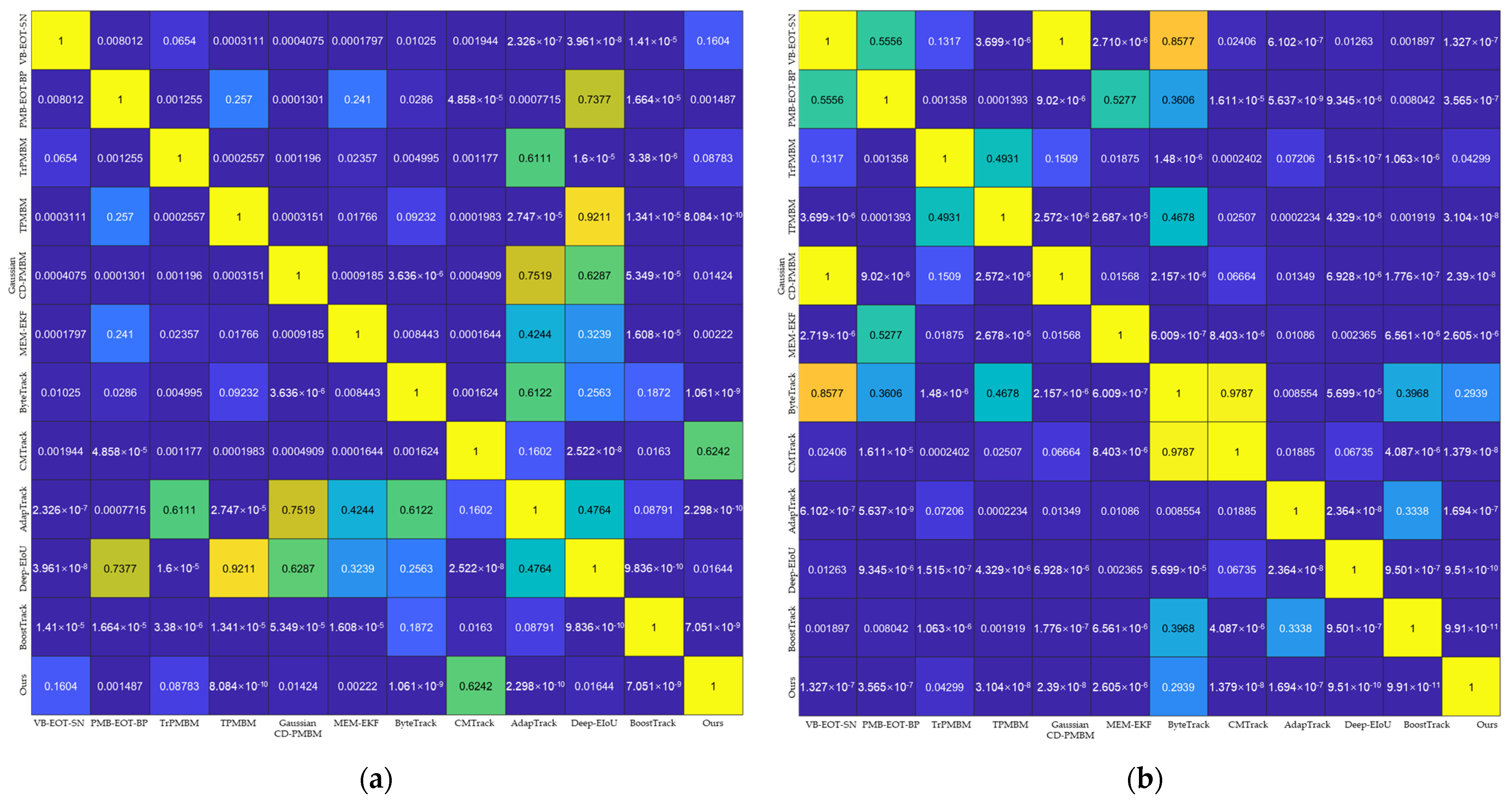
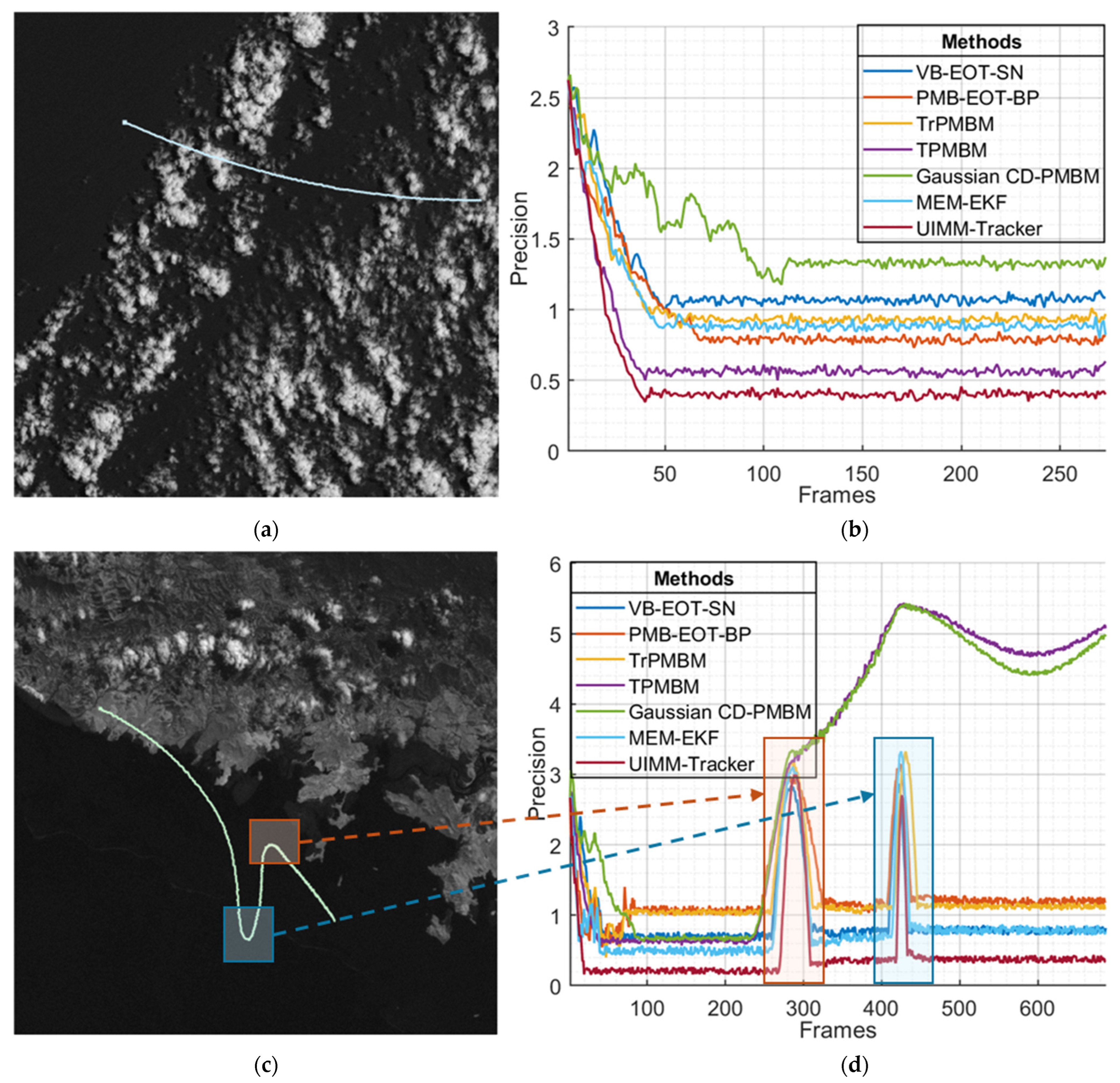
4.2.1. Quantitative Analysis

To comprehensively compare the overall performance and applicability of various methods, we summarize the average values of all metrics across all sequences in Table 1 and report the MOTA and precision metrics of different methods on sequences 1 to 10 (detailed descriptions of the sequences are provided in Table 2) in Table 3. As observed in Table 1, the UIMM-Tracker achieves the best performance in tracking, association, and localization. Compared to the second-ranked traditional algorithm TPMBM, the UIMM-Tracker improves MOTA and HOTA by 0.3% and 0.4%, respectively, while reducing IDs and precision by 3 and 0.78, respectively. Compared to the optimal deep-learning method AdapTrack, although the UIMM-Tracker shows a 0.5% decrease in MOTA, it achieves a 1.5% improvement in HOTA and reduces IDs and precision by 7 and 1.1, respectively. These improvements benefit from the adaptability of the IMM motion model, the autonomous adjustment capability of the dynamic Markov transition matrix, and the accurate representation of observation noise through the measurement of detection uncertainty.
According to the evaluation results in Table 2 for different sequences, the UIMM-Tracker achieves the best performance on sequences with varying target motion states (Seq3, Seq5, Seq6, Seq7, Seq8, and Seq10). For sequences with highly maneuvering targets (Seq5, Seq8, and Seq10), the proposed method also performs best, while the second-best methods, including AdapTrack, TPMBM, and MEM-EKF, vary across sequences. This indicates that other methods are limited to specific scenarios, whereas the proposed method demonstrates stronger generalization ability due to the integration of detection uncertainty measurement, the IMM model, association cost calculation with a joint strategy, and the dynamic Markov transition matrix. It satisfies application requirements under diverse conditions, including different backgrounds, target motion states, and target scales. Notably, the proposed method achieves the highest localization accuracy across all sequences. This is attributed to the use of multiple models and the dynamic Markov transition matrix, which aligns the state prediction process more closely with the actual target motion model, improving prediction accuracy. Moreover, accurate measurement of detection uncertainty ensures a precise representation of the true distribution of observations, enhancing the accuracy of the state update process.
To comprehensively compare the performance differences between our algorithm and the comparison methods, we use significance tests to assess the statistical significance of the experimental results, employing t-tests to analyze mean differences among various methods. According to Table 2, the means of the UIMM-Tracker in MOTA and precision metrics are significantly higher than those of the comparison methods. The visualization of p-value statistics is shown in Figure 5, indicating that the p-values for both metrics between our method and others are close to zero, demonstrating statistical significance in algorithm differences. Additionally, to ensure the robustness of the results, we conducted an ANOVA analysis to verify the interactions among multiple metrics. As shown in Figure 6, the analysis results further support the conclusions of the t-test, confirming that the differences between our method and the comparison methods are statistically significant. This confirms that the impact of the experimental treatment on metrics is not due to random factors but directly reflects differences in tracker performance. Therefore, the UIMM-Tracker method demonstrates significant superiority.

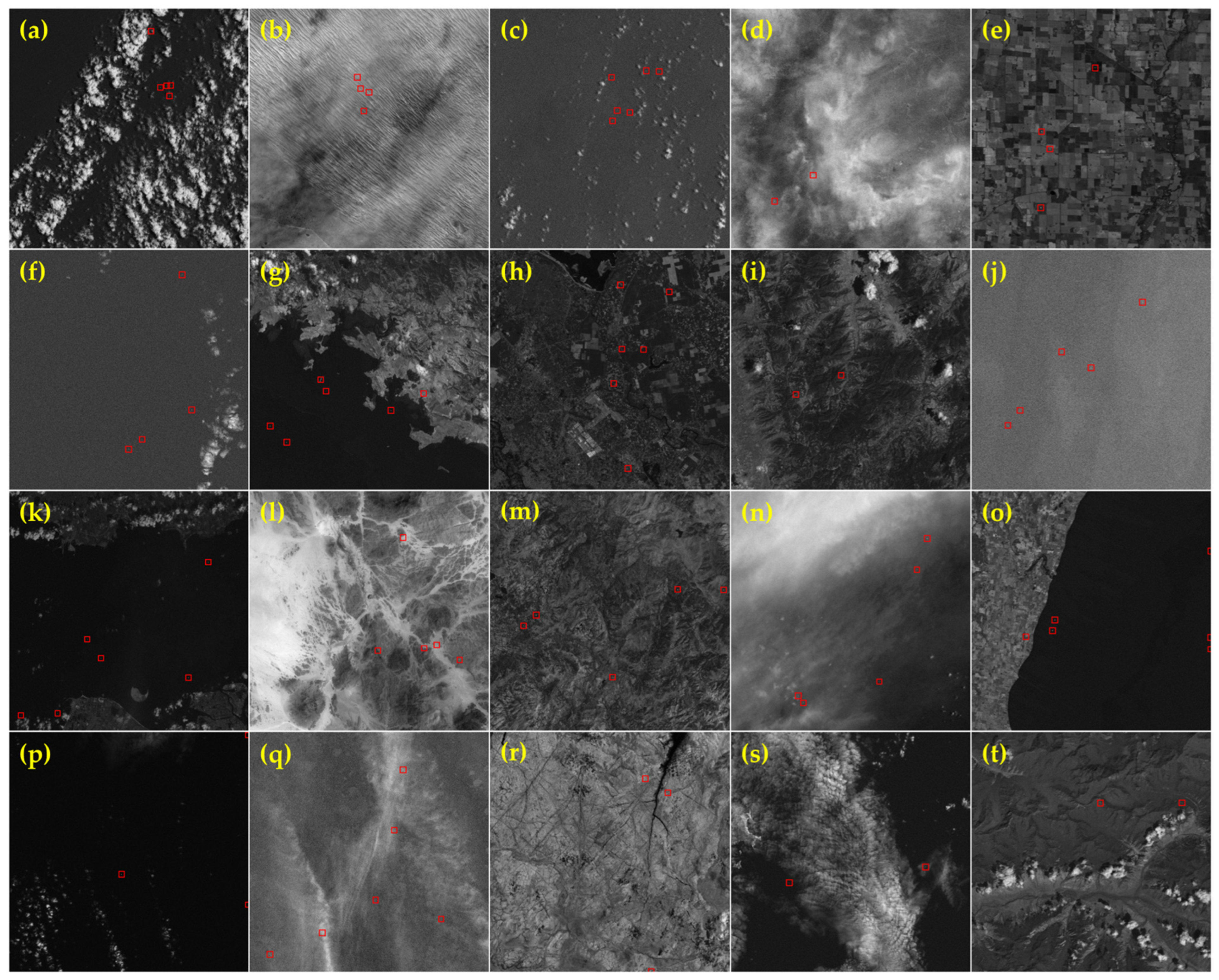
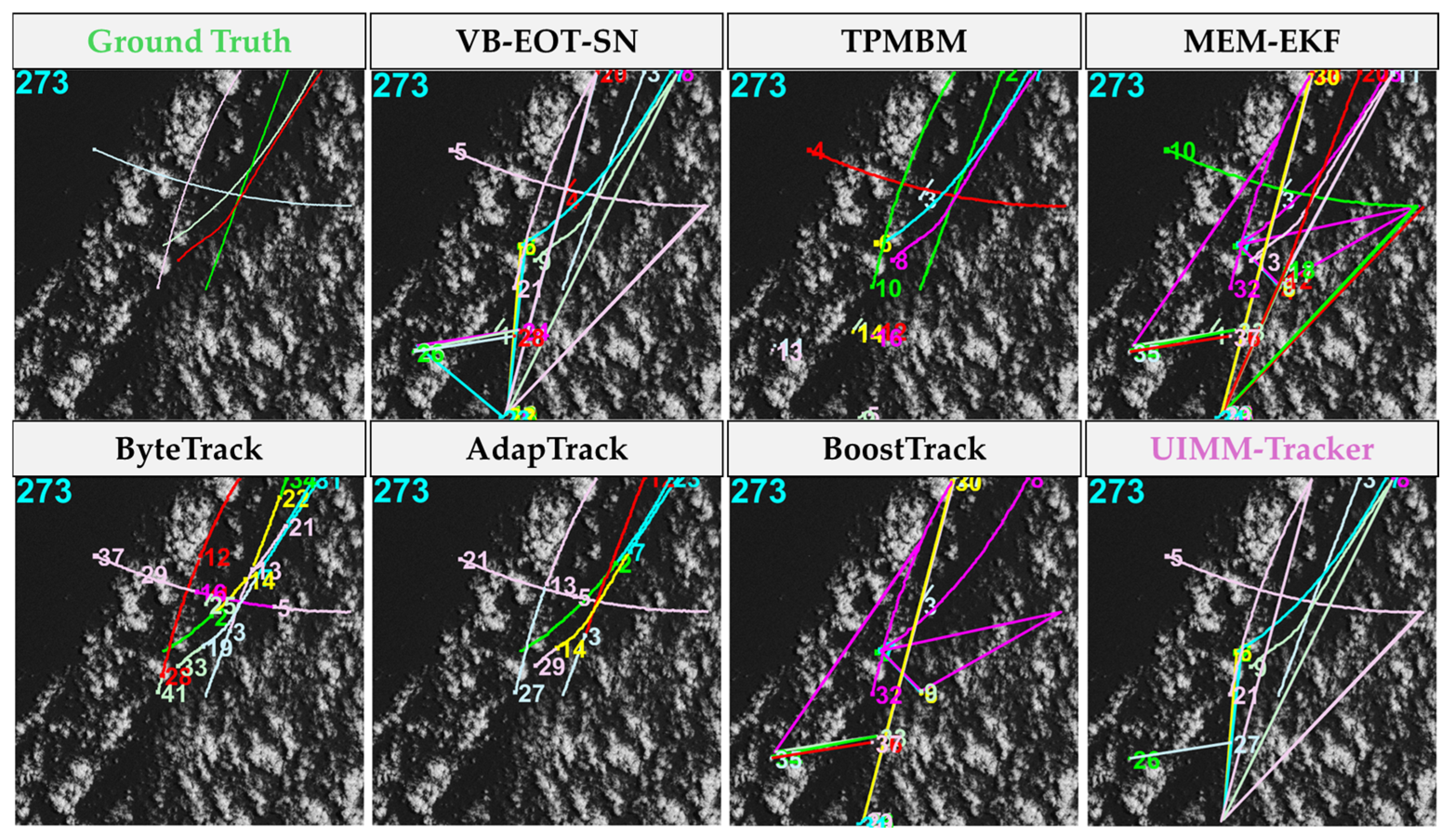
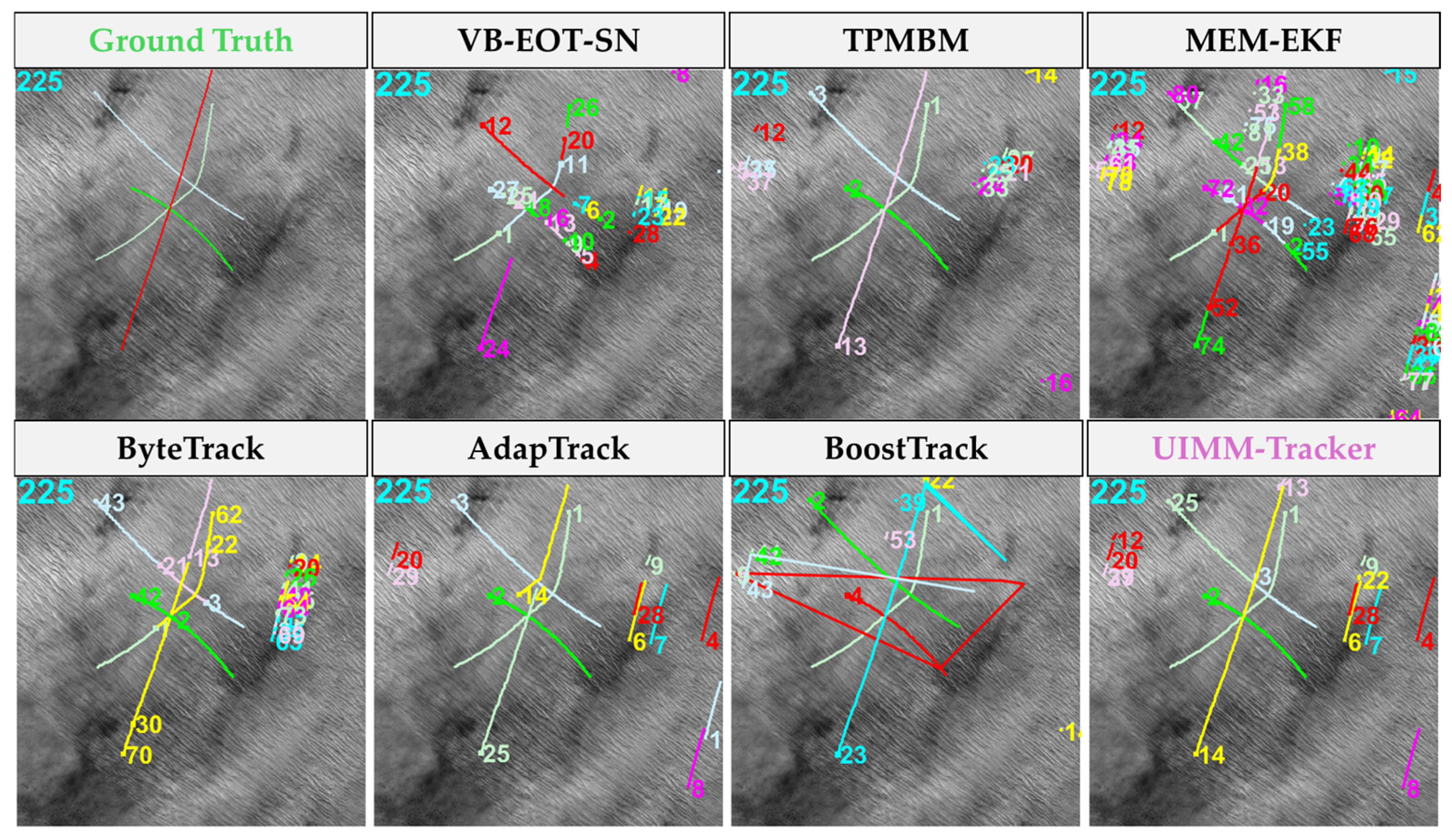
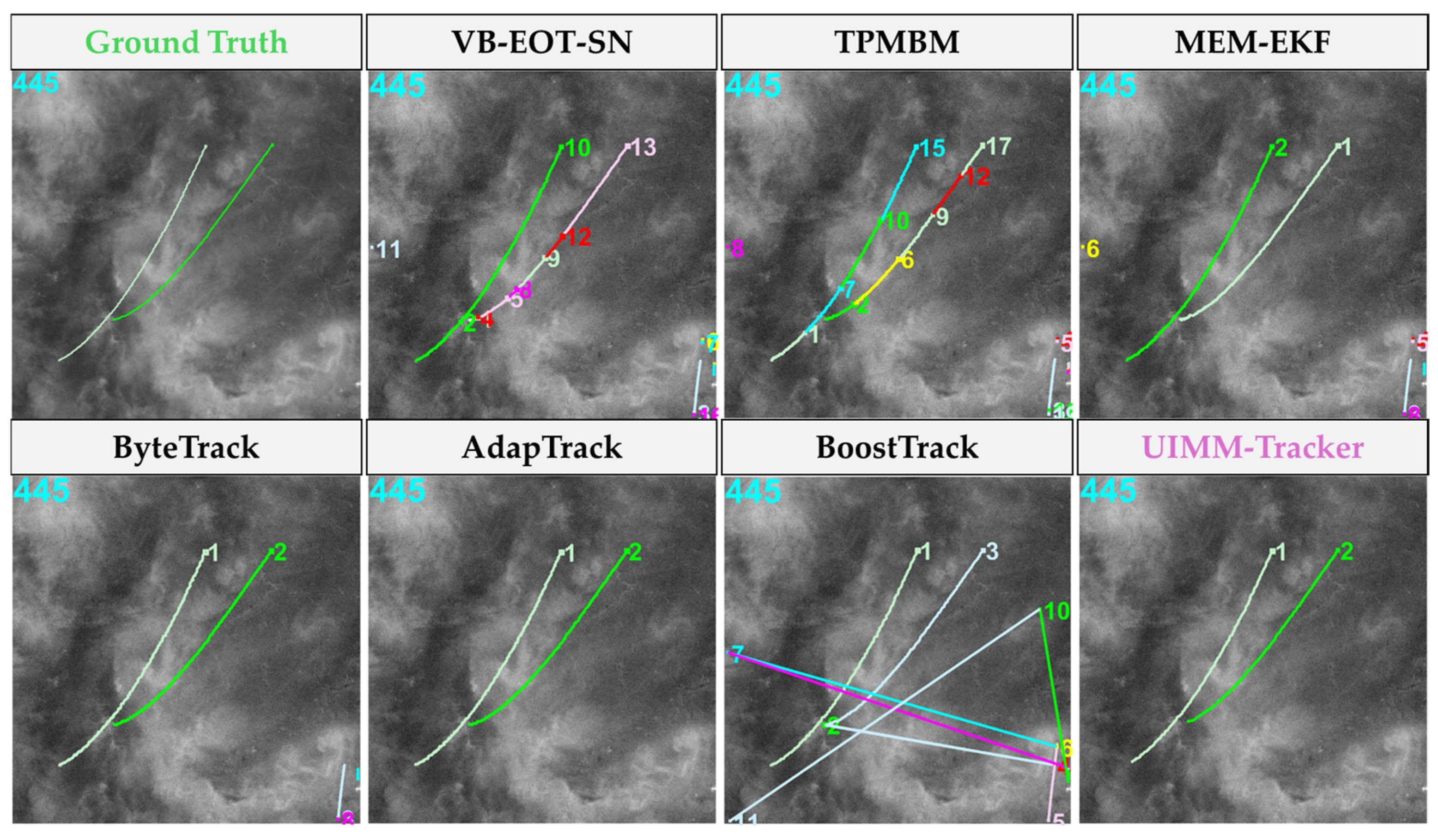
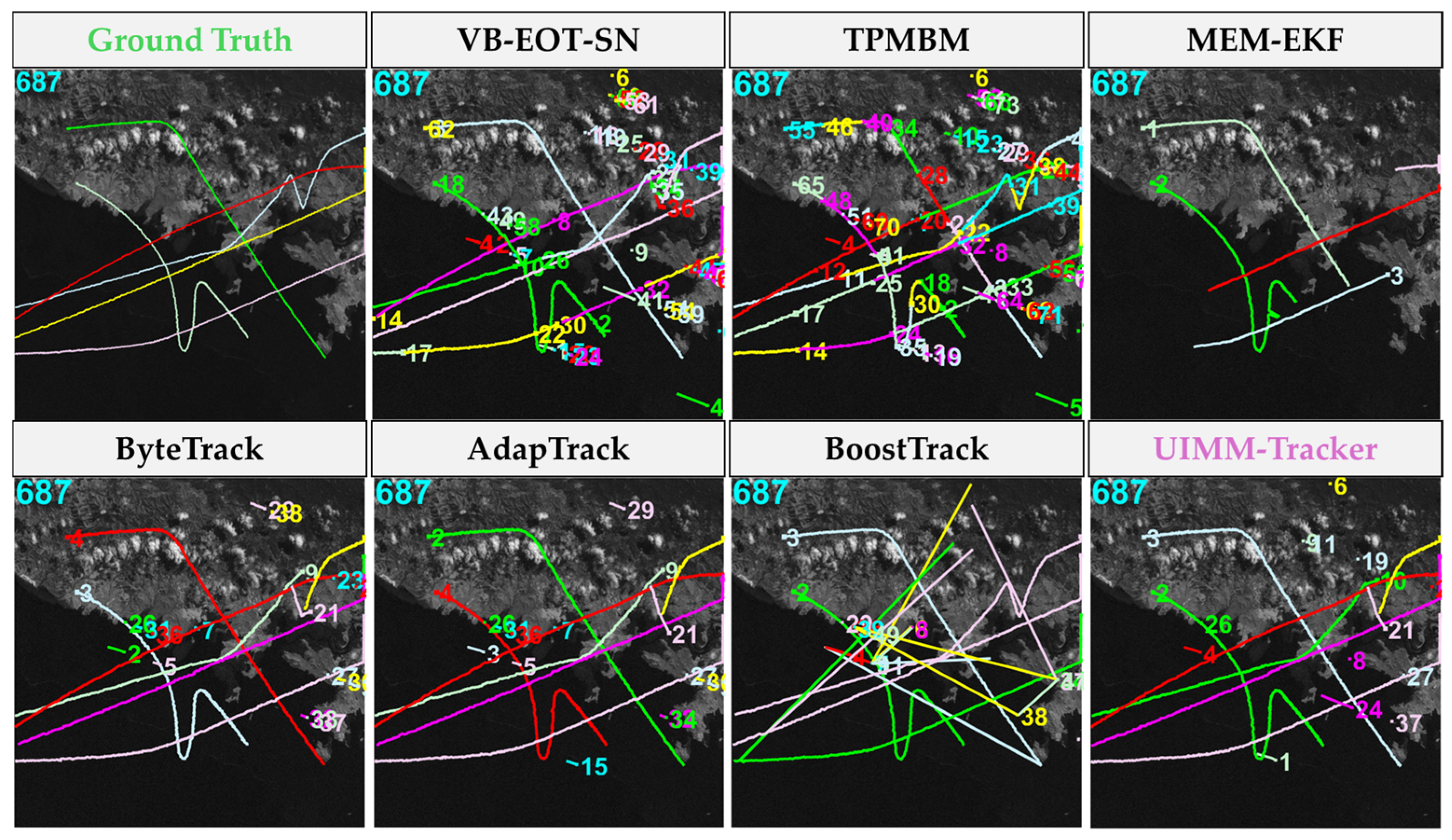
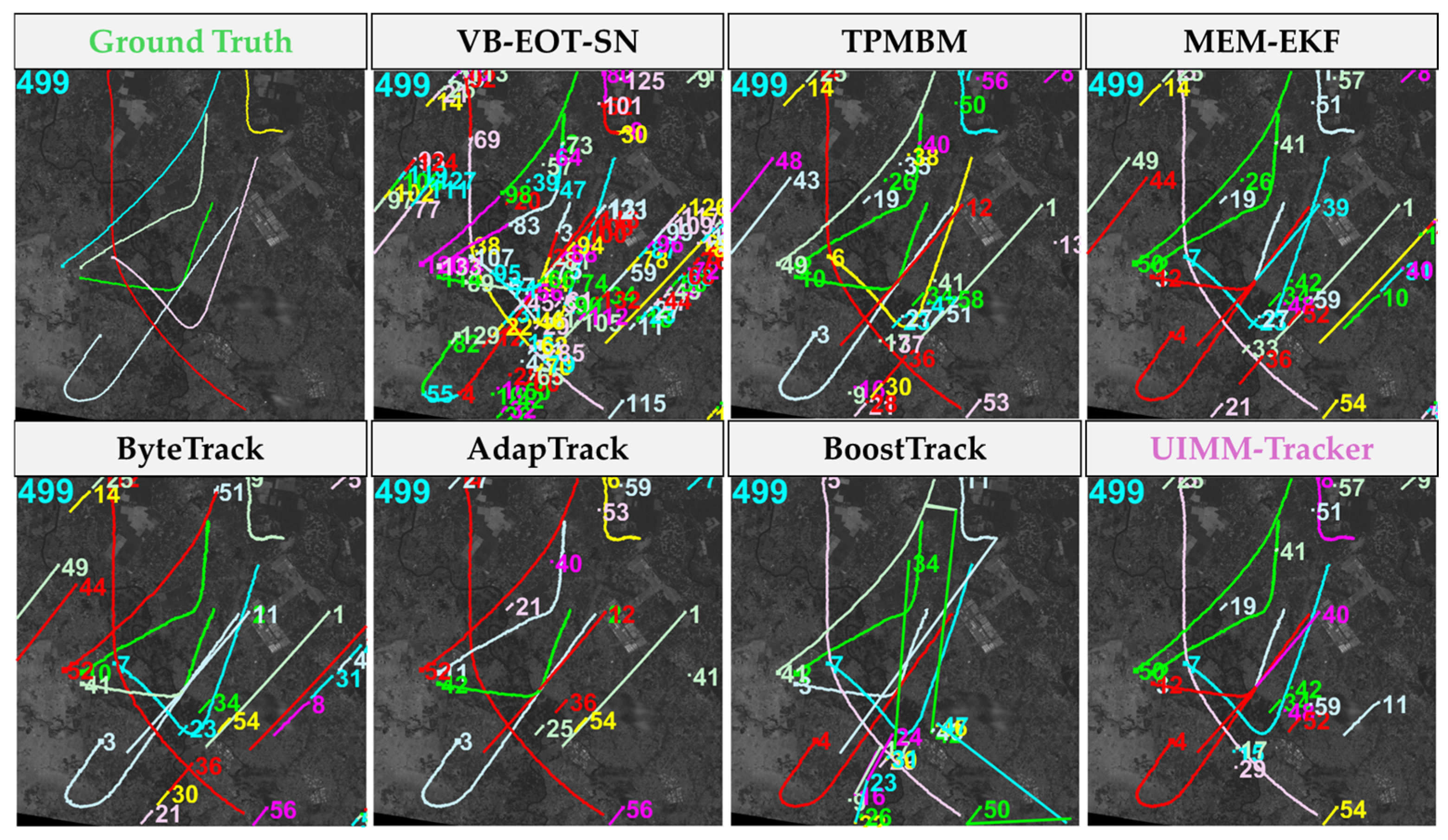
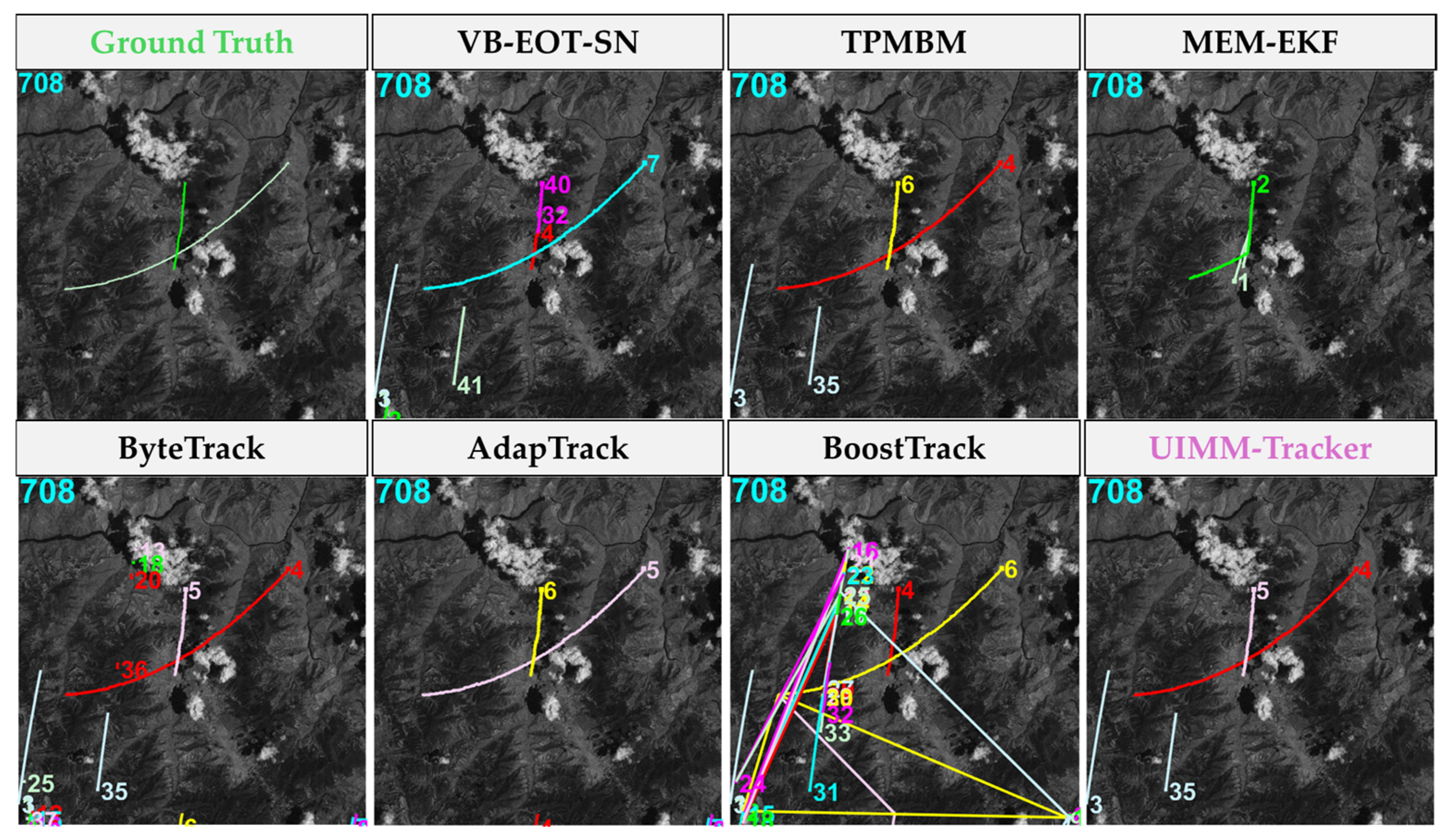
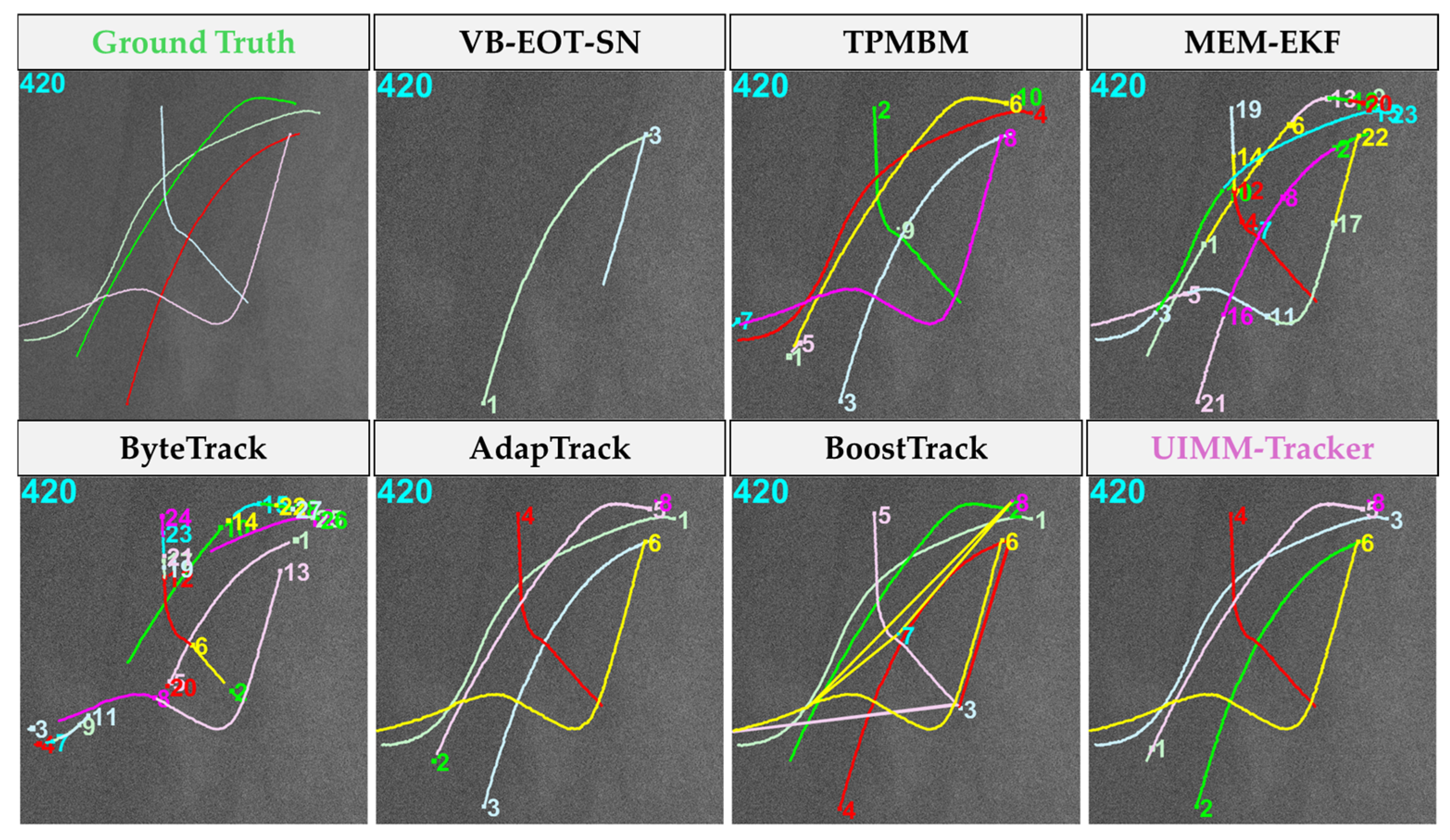
4.2.2. Qualitative Analysis

To intuitively demonstrate the advantages of the UIMM-Tracker in scenario adaptability and tracking performance, we visualize the tracking results of different trackers on the 10 sequences listed in Table 2 in Section 4.2.1, as shown in Figure 7, Figure 8, Figure 9, Figure 10, Figure 11, Figure 12, Figure 13, Figure 14, Figure 15 and Figure 16.
The results indicate that the UIMM-Tracker adapts well to various complex environments, target motion states, and ID switches. For example, in Figure 7, VB-EOT-SN and MEM-EKF produce more mismatches, while the UIMM-Tracker generates fewer erroneous trajectories. In Figure 8, due to a large number of false positives caused by the striped background during detection coupled with background motion, other methods produce more incorrect trajectories, whereas UIMM-Tracker keeps these errors at a lower level. In Figure 9, the motion of fragmented clouds and temporal brightness variations lead methods like BoostTrack to incorrectly associate cloud motion with targets, resulting in numerous ID switches. However, UIMM-Tracker robustly tracks the targets. In Figure 10, strong noise interferes with detection results, causing discontinuities in the detected points of trajectories. Consequently, methods like MEM-EKF produce more ID switches, while UIMM-Tracker achieves the best tracking performance due to its multi-model configuration. In Figure 11, methods like TPMBM generate continuous erroneous trajectory segments, whereas UIMM-Tracker’s unique association strategy effectively suppresses clutter-induced trajectories. In Figure 12, due to trajectory interactions and limitations in detector capability, VB-EOT-SN produces errors in tracked target trajectories, while UIMM-Tracker adapts well to such situations, achieving the best tracking results. In Figure 13, the high contrast of the sea–land boundary and occasional satellite motion result in numerous erroneous trajectories. The proposed method demonstrates the best clutter trajectory suppression capability. Due to the presence of highly maneuvering targets, TPMBM fails to track the target during its initial maneuver, causing ID switches, whereas UIMM-Tracker maintains stable tracking. In Figure 14, the motion states of each target vary, and methods using a single-motion model lead to frequent ID switches. The proposed method achieves continuous target tracking over long time spans. In Figure 15, trajectory intersections cause MEM-EKF to associate two targets as one, while UIMM-Tracker effectively utilizes prior state estimates of each target to prevent trajectory interference. In Figure 16, due to targets being submerged in a noisy background, MEM-EKF and ByteTrack struggle to accurately match targets, resulting in erroneous associations and ID switches. UIMM-Tracker consistently tracks targets stably while maintaining fewer erroneous trajectories.
In summary, due to the unique design of the UIMM-Tracker in model probability transitions and data association, it adapts to complex environmental backgrounds and various target motion states while maintaining low error associations, ultimately achieving the best overall performance compared to other methods.
The analysis of single targets with both simple and complex maneuvering states evaluates the time-varying precision of different methods, as shown in Figure 17. From Figure 17a,b, it is evident that all methods successfully track simple trajectories. Although MEM-EKF converges faster, its precision is lower compared to methods like PMP-EOT-BP. The TrPMBM method ranks average among all methods in both convergence speed and precision. UIMM-Tracker achieves the best precision and the fastest convergence, owing to the IMM model with a dynamic Markov transition matrix, which autonomously updates the current estimate based on the target’s historical motion states. Instead of predicting the target state using a single-motion equation, it describes target motion as a weighted combination of multiple basic motions, significantly enhancing algorithm performance.
From Figure 17c,d, it is observed that Gaussian CD-PMBM and TPMBM initially succeed in tracking the target but fail during the first strong maneuver, with their tracking trajectories gradually deviating from the ground truth. Compared to other methods that successfully track the target, UIMM-Tracker achieves the best tracking precision. Whether before the target maneuver or after the first and second maneuvers, UIMM-Tracker converges the fastest, fully demonstrating the effectiveness of the proposed method.

4.2.3. Efficiency Comparison

Table 4 presents the time required by different algorithms to process one frame. For a fair comparison, deep-learning methods perform inference on the CPU. Deep-learning methods exhibit faster runtime compared to traditional methods but require significant time investment during the training phase. Compared to traditional methods, UIMM-Tracker achieves a processing time of 2.81 s per frame, demonstrating higher overall efficiency. MEM-EKF and VB-EOT-SN rank as the top two in speed, but their performance is suboptimal. Our method processes each frame only 0.16 s slower than VB-EOT-SN yet delivers significantly better performance. Additionally, compared to the second-ranked TPMBM method in terms of performance, our method offers a substantial advantage in processing time, highlighting its ability to effectively balance efficiency and speed.
The computational complexity of the UIMM-Tracker depends on the number of targets N t , the number of motion models M , the state dimension n x , the measurement (detection result) dimension n z , and the number of sigma points 2 n x + 1 . During the input data interaction phase, each target requires the calculation of the model transition probability matrix M × M times. Cholesky decomposition is used to generate sigma points for covariance calculation with a complexity of O ( n x 3 ) . Therefore, the computational complexity for N t targets in the data interaction phase is O ( M 2 N t n x 3 ) . In the state prediction phase, each sigma point requires n x × n x calculations to obtain the predicted value, resulting in a computational complexity of O ( 2 ( n x + 1 ) n x 2 ) . The computational complexity for covariance prediction is O ( n x 3 ) . Therefore, the total complexity for M models and N t targets is O ( M N t n x 3 ) . The data association phase uses the Hungarian algorithm, with a computational complexity of O ( N t 3 ) . In the measurement update phase, the cross-covariance matrix requires n z × n z calculations for each sigma point, with a complexity of O ( 2 ( n x + 1 ) n z 2 ) . The complexity for the inversion of the measurement covariance matrix to compute the Kalman gain is O ( n z 3 ) . Therefore, the total complexity for M models and N t targets is O ( M N t ( n x 3 + 2 ( n x + 1 ) n z 2 ) ) . In the model probability update and fusion phase, the likelihood functions for each model and the updated model probabilities are calculated. The likelihood function calculation involves the inversion of the covariance matrix, with a computational complexity of O ( M N t n z 3 ) . Each target requires M calculations to update model probabilities with a complexity of O ( M N t ) . Therefore, the total complexity for this phase is O ( M N t n z 3 ) + O ( M N t ) . The dynamic adjustment of Markov transition probabilities is proportional to the matrix size, requiring M × M calculations, resulting in a complexity of O ( M 2 ) . Considering all the aforementioned processes, the overall computational complexity is approximately M N t O ( n x 3 + n z 3 ) .

4.3. The Ablation Study

4.3.1. Impact of Detection Uncertainty

To evaluate the impact of detection uncertainty on the UIMM-Tracker, we design the following three experiments to verify the algorithm’s performance:
(1) Without R k , it is simply set to 0. In this case, the association process does not consider the impact of uncertainty, which is used to evaluate the effect of observation noise on target tracking performance.
(2) R k from prior, where R k = diag ( 0.09 , 0.09 , 0.16 , 0.16 ) . In this case, the association process does not consider the impact of uncertainty, which is used to evaluate the effect of given observation noise on target tracking performance.
(3) R k from detections, where R k is measured from detection results and used as input to the tracking algorithm, which is used to evaluate the performance of the target tracking algorithm under accurate observation noise.
The experimental results on the impact of detection uncertainty on the performance of target tracking algorithms are shown in Table 5. The following conclusions can be drawn:
(1) When the observation noise R k is not provided, the algorithm exhibits the worst performance, with MOTA, HOTA, AssA, and IDF1 metrics decreasing by 5.2%, 5.5%, 5.9%, and 10.4%, respectively, while IDs and precision increase by 17 and 0.43, respectively. The algorithm’s performance is severely degraded at the tracking and association levels, and significant errors are introduced at the localization level. This is because observation systems are inherently non-ideal, and observation noise must be included in the measurement and prediction process. Without R k , the observed values deviate significantly from the true values, disrupting the data association process and causing association errors. This leads to degraded performance in target tracking and association, resulting in incorrect state updates, erroneous state estimation, and reduced target localization accuracy.
(2) When the observation noise is provided a priori, the algorithm’s performance is slightly lower compared to when the noise is obtained through measurement. This is due to the inaccuracy of the given noise. Although the provided noise partially reflects the distribution range of the observations, it does not represent the true distribution but rather an approximation based on human experience. As a result, significant deviations still exist between the observed and actual values, leading to data association errors. Additionally, under such conditions, the cost function in the association algorithm does not account for the distribution range of the cost values or additional cost computation methods, further impacting the performance of target association.
(3) The observation noise R k obtained through measurement based on detection results achieves the best performance. Compared to the observation noise provided a priori, the algorithm improves by 0.6%, 1.1%, 0.3%, and 0.7% in MOTA, HOTA, AssA, and IDF1 metrics, respectively, while IDs and precision decrease by 3 and 0.11, respectively. This is because the detection results serve as the observations for the multi-object tracking system, inherently incorporating the imaging system’s intrinsic errors and the detection algorithm’s localization errors, which are ultimately presented in the form of multiple bounding boxes. The covariance measurements obtained during the non-maximum suppression process effectively represent the fusion of all these errors, providing clear and accurate observation noise inputs for the multi-object tracking algorithm. This minimizes association errors to the greatest extent, supplies accurate observations for state updates, and ultimately ensures the accuracy of target localization.

4.3.2. The Impact of the Markov Transition Matrix

To evaluate the impact of the Markov transition matrix on the UIMM-Tracker, we design the following five experiments to verify the algorithm’s performance:
(1) A priori transition matrix M k = 0.8 , 0.1 , 0.1 ; 0.1 , 0.8 , 0.8 ; 0.1 , 0.1 , 0.8 is used to evaluate the target tracking performance of the IMM algorithm under fixed model transition probabilities.
(2) A dynamic Markov transition matrix is employed without considering the dynamic modulation effect of the state measurement error e p ˜ k j on M k to evaluate the impact of modulation of e p ˜ k j on target tracking performance.
(3) A dynamic Markov transition matrix is employed without considering the dynamic modulation effect of the model likelihood Λ ˜ k j on M k to evaluate the impact of modulation of Λ ˜ k j on target tracking performance.
(4) A dynamic Markov transition matrix is employed without considering the dynamic modulation effect of the model probability rate of change ρ k j on M k to evaluate the impact of modulation of ρ k j on target tracking performance.
(5) A dynamic Markov transition matrix is employed comprehensively considering the dynamic modulation effects of e p ˜ k j , Λ ˜ k j and ρ k j on M k to demonstrate the performance advantages of the algorithm.
The experimental results of different Markov transition matrices are shown in Table 6, leading to the following conclusions:
(1) The algorithm performs the worst under the condition of a given Markov transition matrix, with MOTA, HOTA, AssA, and IDF1 decreasing by 10.4%, 8.7%, 4.3%, and 6.3%, respectively, while IDs and precision increase by 24 and 0.26, respectively. This is because the algorithm cannot adaptively track target trajectory changes in maneuvering states based on historical trajectory information, leading to inaccuracies during the multi-model fusion process and resulting in significant state estimation errors. These errors severely impact the processes of association, tracking, and localization, causing a comprehensive decline in all performance metrics.
(2) During the dynamic adjustment of the Markov transition matrix, temporal features incorporating historical information outperform spatial features that only consider current measurements. The tracking results without considering ρ k j are worse than those without considering e p ˜ k j or Λ ˜ k j . Compared to the results without considering e p ˜ k j , the MOTA, HOTA, AssA, and IDF1 metrics decrease by 3.8%, 2.2%, 2.3%, and 2.7%, respectively, while IDs and precision increase by 8 and 0.10, respectively. Compared to the results without considering Λ ˜ k j , the MOTA, HOTA, AssA, and IDF1 metrics decrease by 4.3%, 2.3%, 1.7%, and 2.8%, respectively, while IDs and precision increase by 7 and 0.11, respectively. This is because the model probability rate of change ρ k j represents the degree of variation in the matching between the target motion state and each model, capturing the temporal trend of the target motion model and its affinity with each motion model. This allows for a more comprehensive adjustment of the Markov transition matrix, thereby influencing the processes of target association, tracking, and localization.
(3) The algorithm that comprehensively considers e p ˜ k j , Λ ˜ k j and ρ k j achieves the best tracking performance. Compared to the second-best algorithm, which does not consider e p ˜ k j , it improves MOTA and HOTA by 1.5% and 2.8%, respectively, while reducing IDs and precision by 7 and 0.04, respectively. This fully demonstrates the importance of measurement error, model likelihood probability, and the rate of change in model matching for multi-model data fusion. By incorporating dynamic modulation with multiple factors, the Markov transition matrix better facilitates the matching process between the target and the model under changing motion states. It ensures accuracy while avoiding overly frequent or unreasonable model switches, resulting in a more natural and smoother model transition.

4.3.3. The Impact of Association Methods

To evaluate the impact of the cost calculation method on the UIMM-Tracker, we design the following four experiments to verify the algorithm’s performance:
(1) Excluding uncertainty and not introducing the additional cost U calculation to verify the importance of incorporating uncertainty in the target data association process.
(2) Considering the uncertainty of detection results but excluding scale constraints to verify the impact of the scale consistency assumption on target data association.
(3) Considering the uncertainty of detection results but excluding energy constraints to verify the impact of the energy consistency assumption on target data association.
(4) Considering the uncertainty of detection results and comprehensively incorporating both scale and energy constraints to verify the impact of multiple hypothesis conditions on target data association.
The experimental results of different cost calculation methods are shown in Table 7, leading to the following conclusions:
(1) When uncertainty is not considered, the algorithm achieves the worst tracking performance, with MOTA, HOTA, AssA, and IDF1 decreasing by 3.1%, 4.9%, 5.2%, and 4.8%, respectively, while IDs and precision increase by 14 and 0.23, respectively. This is because, without considering uncertainty, the IoU and NWD hybrid distance is a single value, failing to capture the distribution characteristics of the cost. During Hungarian matching, trajectories and detections that should have uncertain matches are uniquely assigned, resulting in errors in data association and ultimately affecting the algorithm’s performance in association, tracking, and localization.
(2) When considering certainty, the shape consistency constraint of the target is more important than the energy consistency constraint. Compared to the results without U s , the results without U e show a decrease of 0.7% and 2.1% in MOTA and HOTA, respectively, and a decrease of 0.02 in precision. This is because the scale characteristic in cost calculation represents an absolute property of the target, while the energy characteristic, described by the signal-to-clutter ratio, is a relative property between the target and the background. Since the absolute energy property of the target cannot be obtained directly from the image, the scale consistency of the target imposes a stronger constraint.
(3) By jointly considering shape and scale constraints, the algorithm achieves optimal performance. This is because the cost calculation process does not rely solely on the absolute scale invariance assumption or the relative energy invariance assumption but instead leverages the fusion of both. This allows the algorithm to adapt to scenarios that partially deviate from a single assumption, resulting in better performance compared to cases where U s or U e is not considered.

4.3.4. The Impact of Multi-Model

To evaluate the impact of different motion models on the UIMM-Tracker, we design the following four experiments to verify the algorithm’s performance:
(1) CV model only: The CV model is used exclusively to predict and update the target state, adapting to uniform linear motion, to evaluate the algorithm’s performance.
(2) CA model only: The CA model is used exclusively to predict and update the target state, adapting to accelerated linear motion, to evaluate the algorithm’s performance.
(3) CT model only: The CT model is used exclusively to predict and update the target state, adapting to turning motion, to evaluate the algorithm’s performance.
(4) Complete IMM: The CV, CA, and CT models are jointly used to update the target state and perform probabilistic model fusion, meeting the requirements of tracking targets with complex motion states such as accelerated linear motion and turning, thereby verifying the performance advantages of the multi-model tracking algorithm.
The algorithm’s performance under different motion models is shown in Table 8. Since the targets in the scene predominantly exhibit accelerated linear motion, the method considering only the CT model performs the worst. Compared to the method integrating all models, it shows decreases of 19.3%, 21.4%, 16.5%, and 27.1% in MOTA, HOTA, AssA, and IDF1, respectively, while IDs and precision increase by 81 and 1.25, respectively. Similarly, the CA model outperforms the CT model as it accounts for the influence of acceleration. However, it still shows decreases of 1.4%, 1.7%, 2.1%, and 3.4% in MOTA, HOTA, AssA, and IDF1, respectively, with increases of 5 and 0.08 in IDs and precision, respectively. The method integrating all motion models achieves the best performance, as it not only adapts to most accelerated linear motion scenarios but also incorporates the CT model to maintain robustness when the target executes turning maneuvers.
The visualization results of tracking performance for targets under different motion states using various motion models are shown in Figure 18. From Figure 18a,b, it is evident that all models successfully track targets with simple motion states. However, the IMM model converges faster and achieves the highest precision, highlighting the importance of the hybrid model. From Figure 18c,d, it can be observed that all models successfully track highly maneuvering targets. Nevertheless, in terms of convergence speed and localization accuracy, the IMM model demonstrates the best performance, indicating its adaptability for tracking highly maneuvering small infrared targets in remote-sensing images.

4.3.5. Comparison of Tracking Performance Under Different Detection Qualities

As an algorithm based on the TbD paradigm, the UIMM-Tracker’s tracking performance is constrained by detection capabilities. To assess the potential impact of detector performance on tracking algorithm performance, we compare tracking performance using detection results from the RDIAN [72], DNANet [73], LMAFormer [11], SSTNet [74], and LASNet [71] detectors as inputs. As shown in Table 9, experimental results indicate that detector performance directly affects target tracking performance. Higher detection performance enhances tracker capabilities, with metrics such as MOTA, AssA, IDF1, and IDs influenced by both precision and recall. The HOTA metric is mainly affected by recall. Due to the small pixel count occupied by space-based infrared targets, detector positioning accuracy is at the pixel level, and the UIMM-Tracker incorporates detection uncertainty measurements, resulting in consistent precision metrics across different detectors.

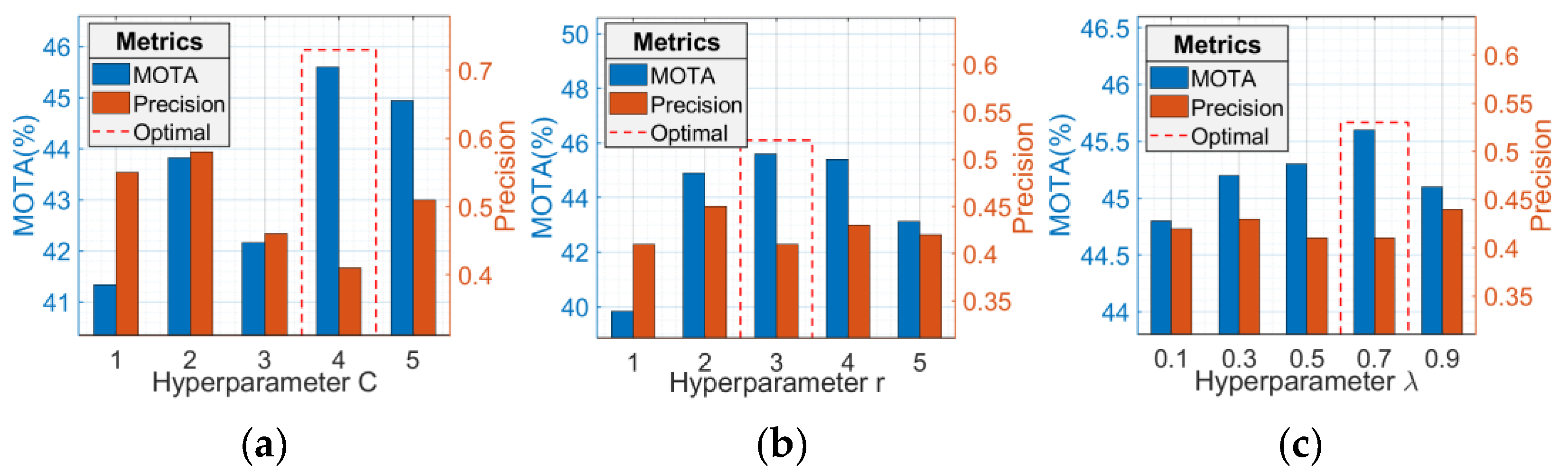
4.3.6. Analysis of Model Hyperparameters

The hyperparameters of the UIMM-Tracker have a direct impact on tracking results, primarily involving the computation of the cost matrix, including the balance parameter C for IoU and NWD costs, the ratio r of background to target radius for calculating the signal-to-clutter ratio, and the weight λ for balancing target scale and energy cost. We conduct separate analyses of each hyperparameter to evaluate the effects of different settings on tracking and state estimation accuracy using the metrics MOTA and precision.
(1) Hyperparameter C for balancing IoU and NWD costs: As shown in Figure 19a, when C ranges from 1 to 5 with a step size of 1, the MOTA and precision metrics are optimal at C = 4. According to Equation (12), when C = A , the weights of IoU and NWD are equally distributed, where A represents the area of the detection box. Given that the average target scale in the dataset is 4 × 4, the best balance between IoU and NWD is achieved at C = 4. When the target scale is smaller than 4 × 4, ( A / C 1 ) > 0 , giving more weight to the NWD cost. Conversely, when the target scale is larger than 4 × 4, ( A / C 1 ) < 0 , causing the cost matrix to be dominated by the IoU measure.
(2) The ratio r of background to target radius in the signal-to-noise ratio calculation: As shown in Figure 19b, when r ranges from 1 to 5 with a step size of 1, the MOTA and precision metrics are optimal at r = 3. This is because each pixel in infrared sensor imaging contains thermal noise. If the background area is too small, the clutter fluctuation σ q s B in Equation (17) mainly reflects thermal noise, failing to accurately characterize the energy difference between the target and background. Conversely, if the value is too large, the calculation of σ q s B introduces additional scene information, leading to inaccurate results.
(3) The balance weight λ for target scale and energy cost: As shown in Figure 19c, when λ ranges from 0.1 to 0.9 with a step size of 0.2, the MOTA and precision metrics are optimal at λ = 0.7. This is because the target scale measures the intrinsic properties of the target, independent of flight speed, maneuvering state, or background, thus offering greater continuity and consistency. In contrast, the energy cost, measured by the signal-to-clutter ratio (SCR), is highly dependent on the background, showing weaker continuity and consistency as the target moves across different backgrounds. Therefore, a value of λ = 0.7 allows the cost calculation to rely more on the scale consistency assumption while also considering energy consistency, thereby enhancing the accuracy of target association.

5. Conclusions

To address challenges such as trajectory interference, association difficulties, and localization inaccuracies in small infrared target tracking under complex remote-sensing backgrounds, this paper introduces detection uncertainty measurements and a dynamic Markov transition matrix into the IMM framework, proposing a method named UIMM-Tracker. The method calculates the covariance of target bounding boxes during the non-maximum suppression (NMS) process as a quantitative description of detection uncertainty. This uncertainty is injected into the observation noise of the IMM to accurately represent the actual distribution of observations, thereby improving the precision of target state estimation. Furthermore, detection uncertainty measurements are incorporated into the data association process. A weighted value of IoU and NWD is adopted as a distance metric, extending the single distance metric between trajectories and detections into a distribution range. Based on this, an auxiliary distance metric is constructed under the assumption of temporal scale and energy invariance of the target, thereby eliminating ambiguous matches between trajectories and detections and enhancing the robustness and accuracy of the data association process. Additionally, this paper proposes a dynamic modulation method for the Markov transition matrix, based on the historical model probability variation rate, current model likelihood probability, and state prediction error. This allows the algorithm to autonomously adjust the weighting of different motion models according to the target’s state changes, enabling adaptation to complex and maneuvering targets and ultimately improving the accuracy of target state prediction. Finally, the proposed algorithm is validated on 20 publicly available complex remote-sensing infrared image sequences. Compared to various classical methods, our approach achieves state-of-the-art performance while maintaining a good balance between accuracy and efficiency.
However, this method still has certain limitations. The assumptions of scale and energy invariance are used as auxiliary means in the cost computation process. When the current cost values are ambiguous, additional assumptions are introduced to resolve the ambiguity. However, the scale of a target is influenced by its inherent size as well as its relative position to the infrared satellite, leading to fluctuations in the target’s size on the image plane within a certain range. The direct assumption of scale invariance cannot fully capture these fluctuations. Similarly, the signal-to-clutter ratio (SCR) of the target also fluctuates with changes in its motion state. The energy invariance assumption simplifies and approximates the modeling of the relative energy relationships between frames, introducing a certain degree of error. Therefore, precise modeling of target scale and energy variations will be a key focus of future research.
In the future, we will focus on studying the interaction and relationships between trajectories and exploring behavior transfer among dense targets to achieve high-precision trajectory determination and reduce interference. Additionally, considering the widespread cloud distribution in space-based infrared imaging scenarios, target trajectories may become discontinuous when passing through cloud layers. To address this, we design a motion-feature-driven appearance re-identification network based on the spatiotemporal characteristics of infrared small targets. This network aims to connect disordered trajectories under cloud-penetrating conditions, enabling the continuous and robust generation of target trajectories.

Author Contributions

Conceptualization, Y.H.; Methodology, Y.H. and W.C.; Software, Y.H. and W.C.; Validation, X.Z., Y.H., Z.X., Q.H. and Y.S.; Formal analysis, J.H.; Investigation, Y.H.; Resources, X.Z.; Data curation, W.C.; Writing—original draft preparation, Y.H.; Writing—review and editing, Y.H., X.Z., Z.X., W.C., J.H., Q.H., Y.S. and W.Z.; Visualization, Y.H., Z.X. and Q.H.; Supervision, W.Z.; Project administration, W.C.; Funding acquisition, X.Z. All authors have read and agreed to the published version of the manuscript.

Funding

This work was supported by the National Natural Science Foundation of China under Grant 62305088 and the China Postdoctoral Science Foundation (Number: 2023M740900).

Data Availability Statement

The benchmark dataset presented in the study is openly available in [55].

Conflicts of Interest

The authors declare no conflicts of interest.

References

  1. Kallenborn, Z.; Plichta, M. Breaking the Shield: Countering Drone Defenses. Jt. Force Q. 2024, 113, 26–35. [Google Scholar]
  2. Jones, M.W.; Kelley, D.I.; Burton, C.A.; Di Giuseppe, F.; Barbosa, M.L.F.; Brambleby, E.; Hartley, A.J.; Lombardi, A.; Mataveli, G.; McNorton, J.R.; et al. State of Wildfires 2023–2024. Earth Syst. Sci. Data 2024, 16, 3601–3685. [Google Scholar] [CrossRef]
  3. Shi, T.; Gong, J.; Hu, J.; Sun, Y.; Bao, G.; Zhang, P.; Wang, J.; Zhi, X.; Zhang, W. Progressive Class-Aware Instance Enhancement for Aircraft Detection in Remote Sensing Imagery. Pattern Recognit. 2025, 164, 111503. [Google Scholar] [CrossRef]
  4. Ren, H.; Zhou, R.; Zou, L.; Tang, H. Hierarchical Distribution-Based Exemplar Replay for Incremental SAR Automatic Target Recognition. IEEE Trans. Aerosp. Electron. Syst. 2025, 61, 6576–6588. [Google Scholar] [CrossRef]
  5. Hu, J.; Wei, Y.; Chen, W.; Zhi, X.; Zhang, W. CM-YOLO: Typical Object Detection Method in Remote Sensing Cloud and Mist Scene Images. Remote Sens. 2025, 17, 125. [Google Scholar] [CrossRef]
  6. Gao, C.; Meng, D.; Yang, Y.; Wang, Y.; Zhou, X.; Hauptmann, A.G. Infrared Patch-Image Model for Small Target Detection in a Single Image. IEEE Trans. Image Process. 2013, 22, 4996–5009. [Google Scholar] [CrossRef]
  7. Huang, Y.; Zhi, X.; Hu, J.; Yu, L.; Han, Q.; Chen, W.; Zhang, W. FDDBA-NET: Frequency Domain Decoupling Bidirectional Interactive Attention Network for Infrared Small Target Detection. IEEE Trans. Geosci. Remote. Sens. 2024, 62, 5004416. [Google Scholar] [CrossRef]
  8. Nicola, M.; Gobetto, R.; Bazzacco, A.; Anselmi, C.; Ferraris, E.; Russo, A.; Masic, A.; Sgamellotti, A. Real-Time Identification and Visualization of Egyptian Blue Using Modified Night Vision Goggles. Rend. Fis. Acc. Lincei 2024, 35, 495–512. [Google Scholar] [CrossRef]
  9. Zhou, X.; Li, L.; Yu, J.; Gao, L.; Zhang, R.; Hu, Z.; Chen, F. Multimodal Aircraft Flight Altitude Inversion from SDGSAT-1 Thermal Infrared Data. Remote Sens. Environ. 2024, 308, 114178. [Google Scholar] [CrossRef]
  10. Zhang, R.; Li, H.; Duan, K.; You, S.; Liu, K.; Wang, F.; Hu, Y. Automatic Detection of Earthquake-Damaged Buildings by Integrating UAV Oblique Photography and Infrared Thermal Imaging. Remote Sens. 2020, 12, 2621. [Google Scholar] [CrossRef]
  11. Huang, Y.; Zhi, X.; Hu, J.; Yu, L.; Han, Q.; Chen, W.; Zhang, W. LMAFormer: Local Motion Aware Transformer for Small Moving Infrared Target Detection. IEEE Trans. Geosci. Remote Sens. 2024, 62, 1–17. [Google Scholar] [CrossRef]
  12. Kou, R.; Wang, C.; Yu, Y.; Peng, Z.; Huang, F.; Fu, Q. Infrared Small Target Tracking Algorithm via Segmentation Network and Multistrategy Fusion. IEEE Trans. Geosci. Remote Sens. 2023, 61, 1–12. [Google Scholar] [CrossRef]
  13. Li, X.; Lv, C.; Wang, W.; Li, G.; Yang, L.; Yang, J. Generalized Focal Loss: Towards Efficient Representation Learning for Dense Object Detection. IEEE Trans. Pattern Anal. Mach. Intell. 2023, 45, 3139–3153. [Google Scholar] [CrossRef]
  14. Xie, X.; Xi, J.; Yang, X.; Lu, R.; Xia, W. STFTrack: Spatio-Temporal-Focused Siamese Network for Infrared UAV Tracking. Drones 2023, 7, 296. [Google Scholar] [CrossRef]
  15. Kuhn, H.W. The Hungarian Method for the Assignment Problem. Nav. Res. Logist. Q. 1955, 2, 83–97. [Google Scholar] [CrossRef]
  16. Psalta, A.; Tsironis, V.; Karantzalos, K. Transformer-Based Assignment Decision Network for Multiple Object Tracking. Comput. Vis. Image Underst. 2024, 241, 103957. [Google Scholar] [CrossRef]
  17. Zou, Z.; Hao, J.; Shu, L. Rethinking Bipartite Graph Matching in Realtime Multi-object Tracking. In Proceedings of the 2022 Asia Conference on Algorithms, Computing and Machine Learning (CACML), Hangzhou, China, 25–27 March 2022; pp. 713–718. [Google Scholar]
  18. Rezatofighi, S.H.; Milan, A.; Zhang, Z.; Shi, Q.; Dick, A.; Reid, I. Joint Probabilistic Data Association Revisited. In Proceedings of the 2015 IEEE International Conference on Computer Vision (ICCV), Santiago, Chile, 7–13 December 2015; pp. 3047–3055. [Google Scholar]
  19. Kim, C.; Li, F.; Ciptadi, A.; Rehg, J.M. Multiple Hypothesis Tracking Revisited. In Proceedings of the 2015 IEEE International Conference on Computer Vision (ICCV), Santiago, Chile, 7–13 December 2015. [Google Scholar]
  20. Yi, K.; Luo, K.; Luo, X.; Huang, J.; Wu, H.; Hu, R.; Hao, W. UCMCTrack: Multi-Object Tracking with Uniform Camera Motion Compensation. Proc. AAAI Conf. Artif. Intell. 2024, 38, 6702–6710. [Google Scholar] [CrossRef]
  21. Hess, R.; Fern, A. Discriminatively Trained Particle Filters for Complex Multi-Object Tracking. In Proceedings of the 2009 IEEE Conference on Computer Vision and Pattern Recognition, Miami, FL, USA, 20–25 June 2009; pp. 240–247. [Google Scholar]
  22. Moraffah, B.; Papandreou-Suppappola, A. Bayesian Nonparametric Modeling for Predicting Dynamic Dependencies in Multiple Object Tracking. Sensors 2022, 22, 388. [Google Scholar] [CrossRef]
  23. Lee, I.H.; Park, C.G. Integrating Detection and Tracking of Infrared Aerial Targets with Random Finite Sets. In Proceedings of the 2024 24th International Conference on Control, Automation and Systems (ICCAS), Jeju, Republic of Korea, 29 October–1 November 2024; pp. 661–666. [Google Scholar]
  24. Wang, C.; Wang, Y.; Wang, Y.; Wu, C.-T.; Yu, G. muSSP: Efficient Min-cost Flow Algorithm for Multi-object Tracking. Neural Inf. Process. Syst. 2019, 32, 423–432. [Google Scholar]
  25. Zhou, H.; Ouyang, W.; Cheng, J.; Wang, X.; Li, H. Deep Continuous Conditional Random Fields With Asymmetric Inter-Object Constraints for Online Multi-Object Tracking. IEEE Trans. Circuits Syst. Video Technol. 2019, 29, 1011–1022. [Google Scholar] [CrossRef]
  26. Bozorgtabar, B.; Goecke, R. Efficient Multi-Target Tracking via Discovering Dense Subgraphs. Comput. Vis. Image Underst. 2016, 144, 205–216. [Google Scholar] [CrossRef]
  27. Yang, Z.; Nie, H.; Liu, Y.; Bian, C. Robust Tracking Method for Small and Weak Multiple Targets Under Dynamic Interference Based on Q-IMM-MHT. Sensors 2025, 25, 1058. [Google Scholar] [CrossRef] [PubMed]
  28. Wang, Y.; Li, R.; Zhang, D.; Li, M.; Cao, J.; Zheng, Z. CATrack: Condition-Aware Multi-Object Tracking with Temporally Enhanced Appearance Features. Knowl.-Based Syst. 2025, 308, 112760. [Google Scholar] [CrossRef]
  29. Huang, M.; Li, X.; Hu, J.; Peng, H.; Lyu, S. Tracking Multiple Deformable Objects in Egocentric Videos. In Proceedings of the 2023 IEEE/CVF Conference on Computer Vision and Pattern Recognition (CVPR), Vancouver, BC, Canada, 17–24 June 2023; pp. 1461–1471. [Google Scholar]
  30. Zhang, J.; Wang, H.; Cui, F.; Liu, Y.; Liu, Z.; Dong, J. Research into Ship Trajectory Prediction Based on An Improved LSTM Network. J. Mar. Sci. Eng. 2023, 11, 1268. [Google Scholar] [CrossRef]
  31. Ma, J.; Chen, X.; Bao, W.; Xu, J.; Wang, H. MADiff: Motion-Aware Mamba Diffusion Models for Hand Trajectory Prediction on Egocentric Videos. arXiv 2024, arXiv:2409.02638. [Google Scholar] [CrossRef]
  32. Qin, Z.; Zhou, S.; Wang, L.; Duan, J.; Hua, G.; Tang, W. MotionTrack: Learning Robust Short-Term and Long-Term Motions for Multi-Object Tracking. In Proceedings of the 2023 IEEE/CVF Conference on Computer Vision and Pattern Recognition (CVPR), Vancouver, BC, Canada, 17–24 June 2023; pp. 17939–17948. [Google Scholar]
  33. Li, X.; Liu, D.; Wu, Y.; Wu, X.; Zhao, L.; Gao, J. Fast-Poly: A Fast Polyhedral Framework For 3D Multi-Object Tracking. IEEE Robot. Autom. Lett. 2024, 9, 10519–10526. [Google Scholar] [CrossRef]
  34. Hua, B.; Yang, G.; Wu, Y.; Chen, Z. Angle-Only Target Tracking Method for Optical Imaging Micro-/Nanosatellite Based on APSO-SSUKF. Space Sci. Technol. 2022, 2022, 9898147. [Google Scholar] [CrossRef]
  35. Yu, C.; Feng, Z.; Wu, Z.; Wei, R.; Song, B.; Cao, C. HB-YOLO: An Improved YOLOv7 Algorithm for Dim-Object Tracking in Satellite Remote Sensing Videos. Remote Sens. 2023, 15, 3551. [Google Scholar] [CrossRef]
  36. Wang, B.; Sui, H.; Ma, G.; Zhou, Y. MCTracker: Satellite Video Multi-Object Tracking Considering Inter-Frame Motion Correlation and Multi-Scale Cascaded Feature Enhancement. ISPRS J. Photogramm. Remote Sens. 2024, 214, 82–103. [Google Scholar] [CrossRef]
  37. Yu, Z.; Liu, C.; Liu, L.; Shi, Z.; Zou, Z. MetaEarth: A Generative Foundation Model for Global-Scale Remote Sensing Image Generation. IEEE Trans. Pattern Anal. Mach. Intell. 2025, 47, 1764–1781. [Google Scholar] [CrossRef]
  38. Revach, G.; Shlezinger, N.; Ni, X.; Escoriza, A.L.; van Sloun, R.J.G.; Eldar, Y.C. KalmanNet: Neural Network Aided Kalman Filtering for Partially Known Dynamics. IEEE Trans. Signal Process. 2022, 70, 1532–1547. [Google Scholar] [CrossRef]
  39. Xinlong, L.; Hamdulla, A. Research on Infrared Small Target Tracking Method. In Proceedings of the 2020 12th International Conference on Measuring Technology and Mechatronics Automation (ICMTMA), Phuket, Thailand, 28–29 February 2020; pp. 610–614. [Google Scholar]
  40. Shan, J.; Yang, Y.; Liu, H.; Liu, T. Infrared Small Target Tracking Based on OSTrack Model. IEEE Access 2023, 11, 123938–123946. [Google Scholar] [CrossRef]
  41. Ye, B.; Chang, H.; Ma, B.; Shan, S.; Chen, X. Joint Feature Learning and Relation Modeling for Tracking: A One-Stream Framework. arXiv 2022, arXiv:2203.11991. [Google Scholar] [CrossRef]
  42. Fan, J.; Wei, J.; Huang, H.; Zhang, D.; Chen, C. IRSDT: A Framework for Infrared Small Target Tracking with Enhanced Detection. Sensors 2023, 23, 4240. [Google Scholar] [CrossRef]
  43. Shuai, B.; Berneshawi, A.; Li, X.; Modolo, D.; Tighe, J. SiamMOT: Siamese Multi-Object Tracking. In Proceedings of the 2021 IEEE/CVF Conference on Computer Vision and Pattern Recognition (CVPR), Nashville, TN, USA, 20–25 June 2021; pp. 12367–12377. [Google Scholar]
  44. Qian, K.; Zhang, S.; Ma, H.; Sun, W. SiamIST: Infrared Small Target Tracking Based on an Improved SiamRPN. Infrared Phys. Technol. 2023, 134, 104920. [Google Scholar] [CrossRef]
  45. Zhang, L.; Lin, W.; Shen, Z.; Zhang, D.; Xu, B.; Wang, K.; Chen, J. Infrared Dim and Small Target Sequence Dataset Generation Method Based on Generative Adversarial Networks. Electronics 2023, 12, 3625. [Google Scholar] [CrossRef]
  46. Xu, Q.; Wang, L.; Sheng, W.; Wang, Y.; Xiao, C.; Ma, C.; An, W. Heterogeneous Graph Transformer for Multiple Tiny Object Tracking in RGB-T Videos. IEEE Trans. Multimed. 2024, 26, 9383–9397. [Google Scholar] [CrossRef]
  47. Tang, X.; Zhong, G.; Li, S.; Yang, K.; Shu, K.; Cao, D.; Lin, X. Uncertainty-Aware Decision-Making for Autonomous Driving at Uncontrolled Intersections. IEEE Trans. Intell. Transp. Syst. 2023, 24, 9725–9735. [Google Scholar] [CrossRef]
  48. Chen, M.; Chen, M.; Yang, Y. UAHOI: Uncertainty-Aware Robust Interaction Learning for HOI Detection. Comput. Vis. Image Underst. 2024, 247, 104091. [Google Scholar] [CrossRef]
  49. Kath, H.; Serafini, P.P.; Campos, I.B.; Gouvêa, T.S.; Sonntag, D. Leveraging Transfer Learning and Active Learning for Data Annotation in Passive Acoustic Monitoring of Wildlife. Ecol. Inform. 2024, 82, 102710. [Google Scholar] [CrossRef]
  50. Rong, Q.; Wu, H.; Otkur, A.; Yue, W.; Su, M. A Novel Uncertainty Analysis Method to Improve the Accuracy of Agricultural Grey Water Footprint Evaluation Considering the Influence of Production Conditions. Ecol. Indic. 2023, 154, 110641. [Google Scholar] [CrossRef]
  51. Maleki Varnosfaderani, S.; Forouzanfar, M. The Role of AI in Hospitals and Clinics: Transforming Healthcare in the 21st Century. Bioengineering 2024, 11, 337. [Google Scholar] [CrossRef]
  52. Mays, D.J.; Elsayed, S.A.; Hassanein, H.S. Uncertainty-Aware Multitask Allocation for Parallelized Mobile Edge Learning. In Proceedings of the GLOBECOM 2023—2023 IEEE Global Communications Conference, Kuala Lumpur, Malaysia, 4–8 December 2023; pp. 3597–3602. [Google Scholar]
  53. Zhou, H.; Yu, J.; Yang, W. Dual Memory Units with Uncertainty Regulation for Weakly Supervised Video Anomaly Detection. Proc. AAAI Conf. Artif. Intell. 2023, 37, 3769–3777. [Google Scholar] [CrossRef]
  54. Ying, X.; Xiao, C.; Li, R.; He, X.; Li, B.; Li, Z.; Wang, Y.; Hu, M.; Xu, Q.; Lin, Z.; et al. Visible-Thermal Tiny Object Detection: A Benchmark Dataset and Baselines 2024. IEEE Trans. Pattern Anal. Mach. Intell. 2025, 47, 6088–6096. [Google Scholar] [CrossRef]
  55. Ying, X.; Liu, L.; Lin, Z.; Shi, Y.; Wang, Y.; Li, R.; Cao, X.; Li, B.; Zhou, S. Infrared Small Target Detection in Satellite Videos: A New Dataset and A Novel Recurrent Feature Refinement Framework. IEEE Trans. Geosci. Remote Sens 2024, 63, 1–18. [Google Scholar] [CrossRef]
  56. Zhang, L.; Lan, J. Extended Object Tracking Using Random Matrix With Skewness. IEEE Trans. Signal Process. 2020, 68, 5107–5121. [Google Scholar] [CrossRef]
  57. Xia, Y.; García-Fernández, Á.F.; Meyer, F.; Williams, J.L.; Granström, K.; Svensson, L. Trajectory PMB Filters for Extended Object Tracking Using Belief Propagation. IEEE Trans. Aerosp. Electron. Syst. 2023, 59, 9312–9331. [Google Scholar] [CrossRef]
  58. Garcia-Fernandez, A.F.; Svensson, L. Tracking Multiple Spawning Targets Using Poisson Multi-Bernoulli Mixtures on Sets of Tree Trajectories. IEEE Trans. Signal Process. 2022, 70, 1987–1999. [Google Scholar] [CrossRef]
  59. Granstrom, K.; Svensson, L.; Xia, Y.; Williams, J.; García-Fernández, Á.F. Poisson Multi-Bernoulli Mixtures for Sets of Trajectories. IEEE Trans. Aerosp. Electron. Syst. 2024, 61, 5178–5194. [Google Scholar] [CrossRef]
  60. García-Fernández, Á.F.; Särkkä, S. Gaussian Multi-Target Filtering with Target Dynamics Driven by a Stochastic Differential Equation. arXiv 2024, arXiv:2411.19814. [Google Scholar] [CrossRef]
  61. Yang, S.; Baum, M. Tracking the Orientation and Axes Lengths of an Elliptical Extended Object. IEEE Trans. Signal Process. 2019, 67, 4720–4729. [Google Scholar] [CrossRef]
  62. Zhang, Y.; Sun, P.; Jiang, Y.; Yu, D.; Weng, F.; Yuan, Z.; Luo, P.; Liu, W.; Wang, X. ByteTrack: Multi-object Tracking by Associating Every Detection Box. In Computer Vision—ECCV 2022; Avidan, S., Brostow, G., Cissé, M., Farinella, G.M., Hassner, T., Eds.; Lecture Notes in Computer Science; Springer Nature: Cham, Switzerland, 2022; Volume 13682, pp. 1–21. ISBN 978-3-031-20046-5. [Google Scholar]
  63. Shim, K.; Hwang, J.; Ko, K.; Kim, C. A Confidence-Aware Matching Strategy For Generalized Multi-Object Tracking. In Proceedings of the 2024 IEEE International Conference on Image Processing (ICIP), Abu Dhabi, United Arab Emirates, 27–30 October 2024; pp. 4042–4048. [Google Scholar]
  64. Shim, K.; Ko, K.; Hwang, J.; Kim, C. Adaptrack: Adaptive Thresholding-Based Matching for Multi-Object Tracking. In Proceedings of the 2024 IEEE International Conference on Image Processing (ICIP), Abu Dhabi, United Arab Emirates, 27 September 2024. [Google Scholar]
  65. Huang, H.-W.; Yang, C.-Y.; Sun, J.; Kim, P.-K.; Kim, K.-J.; Lee, K.; Huang, C.-I.; Hwang, J.-N. Iterative Scale-Up ExpansionIoU and Deep Features Association for Multi-Object Tracking in Sports. In Proceedings of the 2024 IEEE/CVF Winter Conference on Applications of Computer Vision Workshops (WACVW), Waikoloa, HI, USA, 1–6 January 2024; pp. 163–172. [Google Scholar]
  66. Stanojevic, V.D. BoostTrack: Boosting the Similarity Measure and Detection Confidence for Improved Multiple Object Tracking. Mach. Vis. Appl. 2024, 35, 1–15. [Google Scholar] [CrossRef]
  67. Kasturi, R.; Goldgof, D.; Soundararajan, P.; Manohar, V.; Garofolo, J.; Bowers, R.; Boonstra, M.; Korzhova, V.; Zhang, J. Framework for Performance Evaluation of Face, Text, and Vehicle Detection and Tracking in Video: Data, Metrics, and Protocol. IEEE Trans. Pattern Anal. Mach. Intell. 2009, 31, 319–336. [Google Scholar] [CrossRef] [PubMed]
  68. Luiten, J.; Ošep, A.; Dendorfer, P.; Torr, P.; Geiger, A.; Leal-Taixé, L.; Leibe, B. HOTA: A Higher Order Metric for Evaluating Multi-object Tracking. Int. J. Comput. Vis. 2021, 129, 548–578. [Google Scholar] [CrossRef]
  69. Ristani, E.; Solera, F.; Zou, R.; Cucchiara, R.; Tomasi, C. Performance Measures and a Data Set for Multi-target, Multi-camera Tracking. In Computer Vision—ECCV 2016 Workshops; Hua, G., Jégou, H., Eds.; Lecture Notes in Computer Science; Springer International Publishing: Cham, Switzerland, 2016; Volume 9914, pp. 17–35. ISBN 978-3-319-48880-6. [Google Scholar]
  70. Bernardin, K.; Stiefelhagen, R. Evaluating Multiple Object Tracking Performance: The CLEAR MOT Metrics. EURASIP J. Image Video Process. 2008, 2008, 246309. [Google Scholar] [CrossRef]
  71. Chen, S.; Ji, L.; Zhu, S.; Ye, M.; Ren, H.; Sang, Y. Toward Dense Moving Infrared Small Target Detection: New Datasets and Baseline. IEEE Trans. Geosci. Remote Sens. 2024, 62, 5005513. [Google Scholar] [CrossRef]
  72. Sun, H.; Bai, J.; Yang, F.; Bai, X. Receptive-Field and Direction Induced Attention Network for Infrared Dim Small Target Detection With a Large-Scale Dataset IRDST. IEEE Trans. Geosci. Remote Sens. 2023, 61, 5000513. [Google Scholar] [CrossRef]
  73. Li, B.; Xiao, C.; Wang, L.; Wang, Y.; Lin, Z.; Li, M.; An, W.; Guo, Y. Dense Nested Attention Network for Infrared Small Target Detection. IEEE Trans. Image Process. 2023, 32, 1745–1758. [Google Scholar] [CrossRef]
  74. Chen, S.; Ji, L.; Zhu, J.; Ye, M.; Yao, X. SSTNet: Sliced Spatio-Temporal Network with Cross-Slice ConvLSTM for Moving Infrared Dim-Small Target Detection. IEEE Trans. Geosci. Remote Sens. 2024, 62, 5000912. [Google Scholar] [CrossRef]
Figure 1. Technical challenges in space-based infrared remote sensing for small-target tracking: (a) uncertainty in detection results, (b) trajectory interference, and (c) association difficulties.
Remotesensing 17 02052 g001
Figure 2. The inference framework of the UIMM-Tracker within a single time step. Using the target state x ^ k 1 | k 1 1 ~ x ^ k 1 | k 1 N , covariance p ^ k 1 | k 1 1 ~ p ^ k 1 | k 1 N , model probability u k 1 , Markov transition matrix M k 1 , detection uncertainty R k , and detection result d k at time step k − 1 as inputs. Through four steps—state prediction, data association, model update, and data fusion—it outputs the state x k , covariance p k , model probability u k , and Markov transition matrix M k at time step k. The updated state mean x ^ k | k 1 ~ x ^ k | k N and updated state covariance p ^ k | k 1 ~ p ^ k | k N for each model are then used as inputs for the next time step.
Remotesensing 17 02052 g002
Figure 3. The uncertainty of target detection and its impact on cost computation. (a) Uncertainty measurement of detection, (b) uncertainty of IoU, and (c) ambiguous matching in data association.
Remotesensing 17 02052 g003
Figure 4. Examples of infrared remote-sensing satellite small-target tracking datasets. The red boxes indicate the target positions. (at) represent different imaging backgrounds, respectively.
Remotesensing 17 02052 g004
Figure 5. The p-value statistics of different evaluation metrics based on the t-test. (a) MOTA metric and (b) precision metric. The performance differences between the UIMM-Tracker and other methods are significant, fully demonstrating its advantages.
Remotesensing 17 02052 g005
Figure 6. ANOVA analysis results of different methods. (a) MOTA metric and (b) precision metric. ‘’ represents the mean point, and ‘+’ denotes the outliers.
Remotesensing 17 02052 g006
Figure 7. Visualization of tracking results on Sequence 1.
Remotesensing 17 02052 g007
Figure 8. Visualization of tracking results on Sequence 2.
Remotesensing 17 02052 g008
Figure 9. Visualization of tracking results on Sequence 3.
Remotesensing 17 02052 g009
Figure 10. Visualization of tracking results on Sequence 4.
Remotesensing 17 02052 g010
Figure 11. Visualization of tracking results on Sequence 5.
Remotesensing 17 02052 g011
Figure 12. Visualization of tracking results on Sequence 6.
Remotesensing 17 02052 g012
Figure 13. Visualization of tracking results on Sequence 7.
Remotesensing 17 02052 g013
Figure 14. Visualization of tracking results on Sequence 8.
Remotesensing 17 02052 g014
Figure 15. Visualization of tracking results on Sequence 9.
Remotesensing 17 02052 g015
Figure 16. Visualization of tracking results on Sequence 10.
Remotesensing 17 02052 g016
Figure 17. Comparison of time-varying precision across different methods. (a) Ground truth trajectory of a target with simple maneuvering, (b) precision comparison of different methods on a target with simple maneuvering, (c) ground truth trajectory of a target with complex maneuvering, and (d) precision comparison of different methods on a target with complex maneuvering.
Remotesensing 17 02052 g017
Figure 18. Precision comparison of tracking results from different models over time. (a) Ground truth trajectory of a target with simple maneuvering, (b) precision comparison of tracking results from different models on a target with simple maneuvering, (c) ground truth trajectory of a target with complex maneuvering, and (d) precision comparison of tracking results from different models on a target with complex maneuvering.
Remotesensing 17 02052 g018
Figure 19. Results of hyperparameter analysis for the UIMM-Tracker. (a) Hyperparameter C for balancing IoU and NWD costs, with optimal performance achieved at C = 4; (b) ratio r of background to target radius in the signal-to-noise ratio calculation, with the best performance at r = 3; and (c) balance weight λ for target scale and energy cost, with optimal performance when λ = 0.7.
Remotesensing 17 02052 g019
Table 1. The average MOTA (%), HOTA (%), AssA (%), IDF1 (%), IDs (count), and precision (pixels) metrics of different algorithms on each sequence are compared. Red indicates the best value, while blue indicates the second-best. ↑ and ↓ indicate that higher and lower values of the metric are better, respectively.
MethodMOTA ↑HOTA ↑AssA ↑IDF1 ↑IDs ↓Precision ↓
VB-EOT-SN [56]37.246.150.062.1510.82
PMB-EOT-BP [57]41.854.352.563.2440.90
TrPMBM [58]40.552.752.661.6390.93
TPMBM [59]45.355.856.167.2381.19
Gaussian CD-PMBM [60]44.753.955.167.3391.31
MEM-EKF [61]35.044.550.459.7680.74
ByteTrack [62]45.055.254.966.3410.88
CMTrack [63]44.452.953.863.6400.85
AdapTrack [64]46.154.756.267.9421.55
Deep-EIoU [65]43.854.654.765.1430.92
BoostTrack [66]27.233.132.641.9841.48
UIMM-Tracker45.656.255.768.5350.41
Table 2. The target and background description for visual comparison and refined metric evaluation.
SeqFramesSizeTarget NumberTarget ConditionBackground Condition
(1)2731024 × 10245Regular motion
High speed
Small scale
Cloud–Sea background
Complex structure
Gradually changing background
(2)2254Regular motion
Moderate speed
Weak energy
Striped background
Slow movement
Complex structure
(3)1576Trajectory crossing
Varying motion speeds
Small scale
Fragmented cloud background
High noise
Rotating background
(4)4452Continuous acceleration
Weak energy
Small scale
Irregular cloud background
High contrast
High noise
(5)5864High maneuverability
Varying motion speeds
Weak energy
Farmland background
Inconsistent light and shadow
Weak noise
(6)3784Trajectory crossing
Varying motion speeds
Varying scales
Cloud–Sea background
High contrast
High noise
(7)6877Move across backgrounds
Varying motion states
Moderate speed
Land–Sea–Cloud background
Complex terrain
Inconsistent light and shadow
(8)4997Significant differences in speeds
High maneuverability
Presence of dense regions
Urban river background
High-temperature false alarm source
High contrast
(9)7082Slow motion
Fluctuating energy levels
Continuously changing scales
Mountainous background
Uneven illumination
Clutter from structures such as ridges
(10)4205Significant differences in motion states
High maneuverability
Presence of sudden speed changes
Land–Sea background
High noise
Uneven illumination
Table 3. The MOTA (%) and precision (pixels) metrics of different algorithms are compared across 10 challenging datasets. Red indicates the best value, while blue indicates the second-best.
MethodMOTA ↑|Precision ↓
Seq1Seq2Seq3Seq4Seq5Seq6Seq7Seq8Seq9Seq10
VB-EOT-SN [56]37.1|1.0536.2|0.8239.2|0.6941.5|0.7342.4|0.8132.8|0.8940.9|0.7730.6|0.8941.4|0.9430.9|0.91
PMB-EOT-BP [57]44.1|0.6942.1|1.0546.9|0.9838.9|0.9146.5|0.9237.6|0.7945.3|0.8736.9|1.0638.3|0.9238.5|0.71
TrPMBM [58]43.4|0.9337.8|0.8440.3|0.9238.8|0.9644.5|0.9737.9|0.9041.4|0.8937.3|1.0538.8|0.7842.7|0.97
TPMBM [59]48.7|1.3850.3|1.2241.8|0.9340.0|0.9749.7|1.4447.6|0.8245.1|1.1539.9|0.9246.2|1.5044.8|1.26
Gaussian CD-PMBM [60]49.8|1.3144.2|1.3044.4|1.4244.7|1.2248.1|1.1344.3|1.1742.7|1.2840.1|1.4945.6|1.4845.1|1.51
MEM-EKF [61]35.6|0.8636.4|0.6335.8|0.6432.1|0.6840.2|0.6934.8|0.7231.9|0.7038.7|0.8332.3|0.8233.2|0.72
ByteTrack [62]43.9|0.8241.6|0.7946.6|0.8742.8|0.9048.4|0.9247.0|0.9147.7|0.7842.1|1.0445.3|0.7944.6|0.99
CMTrack [63]41.7|0.8943.5|0.9145.0|0.8243.3|0.9447.1|0.7544.8|0.8947.0|0.6941.8|1.0544.5|0.8145.3|0.75
AdapTrack [64]43.1|1.5443.7|1.7046.0|1.8644.8|1.5849.6|1.2548.3|1.3849.2|1.2445.1|1.8346.0|1.6045.2|1.52
Deep-EIoU [65]42.0|0.9944.5|1.1243.0|0.9242.6|0.9345.4|0.9744.1|0.8745.2|0.7442.0|0.9944.3|0.8144.9|0.88
BoostTrack [66]26.6|1.6726.7|1.4827.3|1.6123.6|1.5427.4|1.5430.9|1.4727.1|1.2425.5|1.6927.3|1.3229.6|1.25
UIMM-Tracker40.5|0.5044.8|0.4846.6|0.4344.1|0.4551.2|0.4648.4|0.3448.9|0.3242.4|0.5646.1|0.3345.7|0.35
Table 4. Performance and efficiency comparison of different algorithms. Bold indicates the best value, while the second-best is underlined.
MethodsMOTA ↑HOTA ↑Precision ↓Time (s) ↓
VB-EOT-SN [56]37.246.10.822.65
PMB-EOT-BP [57]41.854.30.909.07
TrPMBM [58]40.552.70.9318.63
TPMBM [59]45.355.81.1917.29
Gaussian CD-PMBM [60]44.753.91.3117.95
MEM-EKF [61]35.044.50.741.71
ByteTrack [62]45.055.20.881.42
CMTrack [63]44.452.90.852.47
AdapTrack [64]46.154.71.551.51
Deep-EIoU [65]43.854.60.920.93
BoostTrack [66]27.233.11.484.18
UIMM-Tracker45.656.20.412.81
Table 5. The impact of different R k acquisition methods on the performance of UIMM-Tracker is analyzed. The optimal values are highlighted in bold.
The Method for Obtaining R k MOTA ↑HOTA ↑AssA ↑IDF1 ↑IDs ↓Precision ↓
Without R k 40.450.749.858.1520.84
R k from prior45.055.155.467.8380.52
R k from detections45.656.255.768.5350.41
Table 6. The impact of different Markov transition matrix construction methods on the performance of the UIMM-Tracker. Bold values indicate optimal results.
Markov Transition Matrix Construction MethodsMOTA ↑HOTA ↑AssA ↑IDF1 ↑IDs ↓Precision ↑
e p ˜ k j Λ ˜ k j ρ k j
35.247.551.462.2590.67
44.153.455.968.1420.45
44.653.555.368.2430.44
40.351.253.665.4500.55
45.656.255.768.5350.41
Table 7. The impact of different cost calculation methods on the performance of the UIMM-Tracker. Bold values indicate optimal results.
Cost Calculation MethodsMOTA ↑HOTA ↑AssA ↑IDF1 ↑IDs ↓Precision ↑
Uncertainty U s U e
----42.551.350.563.7490.64
44.754.454.867.2410.46
45.456.554.367.0390.44
45.656.255.768.5350.41
Table 8. The impact of different motion models on the performance of the UIMM-Tracker. Bold indicates optimal values.
Motion ModelMOTA ↑HOTA ↑AssA ↑IDF1 ↑IDs ↓Precision ↑
CVCACT
39.448.746.258.8650.75
44.254.553.665.1400.49
26.334.839.241.41161.66
45.656.255.768.5350.41
Table 9. Comparison of UIMM-Tracker algorithm performance under different detection inputs. Bold indicates optimal values.
DetectorPrecision (%)Recall (%)MOTA ↑HOTA ↑AssA ↑IDF1 ↑IDs ↓Precision ↓
RDIAN [72]79.9865.8338.446.549.264.8460.41
DNANet [73]80.8471.9742.755.852.467.0450.42
LMAFormer [11]81.0671.2942.655.152.366.9380.40
SSTNet [74]83.9569.5143.353.652.867.2360.43
LASNet [71]85.3273.6445.656.255.768.5350.41
Disclaimer/Publisher’s Note: The statements, opinions and data contained in all publications are solely those of the individual author(s) and contributor(s) and not of MDPI and/or the editor(s). MDPI and/or the editor(s) disclaim responsibility for any injury to people or property resulting from any ideas, methods, instructions or products referred to in the content.

