Impact of Mesoscale Eddies on Acoustic Propagation Under a Rough Sea Surface

Abstract

This study investigates the combined effects of mesoscale eddies and rough sea surfaces on acoustic propagation in the eastern Arabian Sea and Gulf of Aden during summer monsoon conditions. Utilizing three-dimensional sound speed fields derived from CMEMS data, sea surface spectra from the SWAN wave model validated by Jason-3 altimetry, and the BELLHOP ray-tracing model, we quantify their synergistic impacts on underwater sound. A Monte Carlo-based dynamic sea surface roughness model is integrated with BELLHOP to analyze multiphysics interactions. The results reveal that sea surface roughness significantly influences surface duct propagation, increasing transmission loss by approximately 20 dB compared to a smooth sea surface, while mesoscale eddies deepen the surface duct and widen convergence zones by up to 5 km. In deeper waters, eddies shift convergence zones and reduce peak sound intensity in the deep sound channel. These findings enhance sonar performance and underwater communication in dynamic, monsoon-influenced marine environments.

1. Introduction

Underwater acoustic propagation research fundamentally involves solving wave equations in heterogeneous marine environments, with its primary objective being to elucidate how spatiotemporal variations in environmental parameters influence the structure of acoustic fields [1]. Mesoscale oceanic processes—such as eddies, fronts, and internal waves—modify sound speed profiles through thermohaline redistribution [2,3], thereby inducing acoustic path refraction and redistribution of modal energy [4]. Specifically, mesoscale eddies generated by baroclinic instability introduce anomalies in potential vorticity that deform isopycnal surfaces, altering vertical gradients of the sound speed profile. These perturbations affect the distribution of convergence zones within the theoretical framework of waveguide invariants [5,6]. Studies have demonstrated that the presence of mesoscale eddies significantly alters key characteristics of the acoustic field compared to scenarios without such features. These modifications include shifts in convergence zone locations, changes in the order of multipath arrivals, and horizontal refraction phenomena [7]. Furthermore, mesoscale eddies can induce alterations in the structural properties of convergence zones and may lead to the emergence or suppression of surface duct effects [8]. Considerable progress has been made in the development of theoretical models for calculating acoustic fields under rough sea surface conditions, resulting in a variety of well-established theories and numerical methods. Commonly employed approaches include the Kirchhoff approximation, the small-slope approximation [9,10], and the Range-Dependent Acoustic Model (RAM), which is based on parabolic equation methods [11,12]. Research efforts have primarily focused on understanding the impacts of acoustic attenuation, spatiotemporal coherence, and signal time-of-arrival characteristics under such surface conditions.

In the Gulf of Aden, acoustic propagation behavior is governed by monsoon-driven multiscale ocean dynamics. During the summer southwest monsoon (June–September; mean wind speeds exceeding 12 m/s), the Somali Current becomes highly active (surface velocities > 1.5 m/s) [13], giving rise to the Great Whirl eddy via barotropic instability. Argo float observations reveal that this eddy induces thermohaline modifications through vertical mixing, resulting in mixed layer depth anomalies of up to 26.7 m within its core region [1]. Concurrently, enhanced sea surface roughness under monsoonal forcing (significant wave heights reaching 4 m [14]) introduces coupled perturbations through air–sea interactions, forming composite modulation mechanisms that influence underwater acoustic propagation [15].

The coupled effects of mesoscale eddies and sea surface roughness on underwater acoustic propagation have attracted growing attention in recent years [16,17]. Early theoretical models primarily focused on quantifying the sound speed variations induced by eddies using quasi-geostrophic potential vorticity equations [5], whereas more recent investigations have adopted three-dimensional ocean–acoustic coupled frameworks to better resolve these complex interactions.

Mesoscale eddies have been shown to exert a significant influence on underwater sound propagation. A study utilizing three-dimensional temperature and salinity fields from the HYCOM model demonstrated that cold eddies in the Luzon Strait alter the convergence zone structure of the acoustic field, as simulated using the FOR3D acoustic model [18]. Further investigations employing the MITgcm-BELLHOP integrated system revealed that interactions between Luzon cold eddies and tidal currents can shift convergence zones forward by approximately 5 km, with arrival delays of about 0.1 s [19].

Regarding sea surface roughness, research has indicated that it is a dominant factor contributing to acoustic signal attenuation. A comparative analysis of broadband acoustic pressure fields under varying wind conditions concluded that surface roughness plays a primary role, while bubble scattering and Doppler shifts are secondary contributors [20]. Moreover, modeling efforts using Ramsurf in conjunction with PM spectra and Monte Carlo simulations showed that transmission loss increases by 4–6 dB under realistic sea state conditions compared to idealized smooth surface assumptions [21].

Despite these advances, current research faces two major limitations:

(1) Most studies on eddy–acoustic interactions assume idealized smooth sea surfaces, neglecting the coupled effects between vortical flows and wind-driven surface roughness [22].

(2) Traditional PM spectral models fail to accurately represent sea states in topographically complex regions such as the Gulf of Aden, where monsoon-regulated fetch limitations reduce spectral accuracy.

To address these challenges, this study develops a coupled modeling framework that integrates three-dimensional eddy-resolving sound speed fields with sea surface spectra simulated by SWAN (Simulating Waves Nearshore). Through BELLHOP ray tracing simulations, we quantify the synergistic interaction between mesoscale eddies and sea surface roughness on acoustic propagation, providing theoretical support for optimizing underwater detection systems in monsoon-influenced marine environments.

2. Methodology

To accurately characterize sea surface roughness in the target maritime region, the SWAN model was employed as an alternative to the conventional PM spectrum [23]. This approach was integrated with the Monte Carlo method (also referred to as the linear filtering technique) to construct a one-dimensional dynamic sea surface roughness model. The study area has a water depth exceeding 3000 m, thereby fulfilling the assumptions of a deep-water waveguide. Furthermore, BELLHOP’s multi-patch configuration effectively accommodates rough sea surface boundary conditions, making it a suitable tool for acoustic propagation simulations. By parameterizing the upper boundary conditions, the modeling framework systematically incorporates sea surface perturbation effects while maintaining computational stability in deep-water environments.

2.1. Wave Model

The SWAN (Simulating Waves Nearshore) model, developed at Delft University of Technology, is a third-generation spectral wave model that has achieved operational maturity through decades of continuous refinement. Its theoretical foundation is based on the action balance equation derived from principles of energy conservation. The model incorporates the core features of third-generation wave models while specifically addressing hydrodynamic processes in shallow-water environments [24]. The governing equations are solved using a fully implicit finite-difference scheme, which ensures unconditional numerical stability and removes constraints related to spatial grid resolution and temporal step size. The source terms include conventional energy components such as wind input, nonlinear wave–wave interactions, whitecap dissipation, and bottom friction. Additionally, depth-induced wave-breaking mechanisms are incorporated to improve simulation accuracy across coastal-to-offshore transition zones [25,26].

SWAN solves the spectral action balance equation. Although spectral energy density becomes non-conservative in the presence of ambient currents due to Doppler shifting and energy transfer, wave action $N(\sigma ,\theta )$ remains a conserved quantity. It advects with the sum of the intrinsic group velocity and the ambient current velocity. In a Cartesian coordinate system, the wave action balance equation can be expressed as:

$${\displaystyle \frac{\partial }{\partial t}}N+{\displaystyle \frac{\partial }{\partial x}}{C}_{x}N+{\displaystyle \frac{\partial }{\partial y}}{C}_{y}N+{\displaystyle \frac{\partial }{\partial \sigma }}{C}_{\sigma }N+{\displaystyle \frac{\partial }{\partial \theta }}{C}_{\theta }N={\displaystyle \frac{S}{\sigma }}$$

(1)

In the governing equation, the first term on the left-hand side (LHS) represents the temporal variation rate of wave action density. The second and third terms denote the propagation of wave action in the $x$ and $y$ directions of the geographical space, respectively. The fourth term accounts for the advection of wave action in the $\sigma$ space (relative frequency domain) induced by ambient currents and varying water depths. The fifth term describes the refraction-induced redistribution of wave action in the $\theta$ space (directional domain), which arises from depth- and current-driven modifications to wave phase speed. The right-hand side (RHS) $S/\sigma$ encapsulates the source/sink terms, where $S$ aggregates energy inputs and outputs from wind energy transfer $S_{in}$, nonlinear wave–wave interactions $S_{nl}$, bottom friction dissipation $S_{bot}$, whitecap dissipation $S_{wc}$, and depth-induced wave breaking $S_{ds}$.

The governing velocity components in the wave action balance equation are defined as:

$$C_x=c_g\cos \theta +U$$

(2)

$$C_y=c_g\sin \theta +V$$

(3)

$$C_{\sigma }={\displaystyle \frac{\partial \sigma }{\partial t}}+U\cdot \nabla \sigma$$

(4)

$$C_{\theta }=-{\displaystyle \frac{1}{k}}\left({\displaystyle \frac{\partial \sigma }{\partial y}}\sin \theta -{\displaystyle \frac{\partial \sigma }{\partial x}}\cos \theta \right)$$

(5)

The propagation velocities in the wave action balance equation encapsulate distinct physical mechanisms governing spectral evolution. In geographical space, $C_x$ and $C_y$ represent the total advection velocities in the $x$ and $y$ directions, respectively, combining the wave group velocity components ($C_g\cos \theta$ and $C_g\sin \theta$) with ambient current velocities ($U$ and $V$) to resolve wave-energy transport under coexisting wave-current dynamics. In spectral space, $C_{\sigma }$ quantifies the frequency shifting rate in the relative frequency $\sigma$ domain, driven by temporal variations ($\partial \sigma /\partial t$) and spatial gradients of currents or depths ($U\cdot \nabla \sigma$), which collectively induce Doppler-like spectral compression/expansion. Meanwhile, $C_{\theta }$ governs refraction in the directional $\theta$ domain, where depth- or current-induced gradients ($\partial \sigma /\partial x$) redirect wave energy through phase-speed modifications, with the $1/k$ term ($k$: wavenumber) ensuring kinematic consistency with the linear dispersion relation ${\sigma }^2=gk\tanh (kh)$.

2.2. Acoustic Ray Model

Selecting an appropriate sound field model is crucial for accurately investigating the mechanisms of underwater acoustic propagation. Such a model must be capable of capturing the complexities of horizontally varying ocean environments. In the 1980s, Porter and Bucker introduced the Gaussian beam approximation, originally developed in the field of geoacoustics, into underwater acoustics [27]. This innovation facilitated the development of the BELLHOP ray-tracing model, which computes the acoustic field based on a prescribed sound speed profile—a critical determinant of underwater acoustic behavior. Notably, BELLHOP can simulate sound fields in regions such as acoustic shadow zones and focal dispersion areas, where conventional ray theory often fails to provide accurate results. Moreover, the model effectively addresses challenges associated with low-frequency acoustic propagation, thereby enhancing simulation accuracy in these regimes. Owing to its clear physical interpretation and computational efficiency, the BELLHOP model has become a widely used tool in range-dependent underwater acoustic studies [28,29,30,31,32,33,34,35].

The BELLHOP model employs the Gaussian beam method as its core computational approach. This method represents sound propagation using beams of finite width, each characterized by two key parameters: curvature and beam width. The intensity distribution across a beam follows a Gaussian function. The overall sound field generated by a source is approximated as the superposition of contributions from multiple Gaussian beams [36].

The Gaussian beam method simplifies the vector wave equation governing sound propagation into a set of ordinary differential equations: the ray equation and its accompanying parabolic equation:

$${\displaystyle \frac{dr(s)}{ds}}=c(s)\xi (s)$$

(6)

$${\displaystyle \frac{d\xi (s)}{ds}}=-{\displaystyle \frac{1}{c^2(s)}}{\displaystyle \frac{\partial c(s)}{\partial r(s)}}$$

(7)

$${\displaystyle \frac{dz(s)}{ds}}=c(s)\zeta (s)$$

(8)

$${\displaystyle \frac{d\zeta (s)}{ds}}=-{\displaystyle \frac{1}{c^2(s)}}{\displaystyle \frac{\partial c(s)}{\partial z(s)}}$$

(9)

where $c$ is the sound speed, $r(s)$ and $z(s)$ indicate the coordinates of the ray in the column coordinate system, and s represents the arc length in the direction of the ray. Here, the auxiliary variables $\xi (s)$ and $\zeta (s)$ are introduced to write the equation in first-order form. A set of concomitant components, $p(s)$ and $q(s)$, are used to describe the curvature and width of the ray, and they form the accompanying equation for ray tracing:

$$\left\{\begin{array}{l}{\displaystyle \frac{dp}{ds}}=-{\displaystyle \frac{c_{nm}}{c^2(s)}}q(s)\\ {\displaystyle \frac{dq}{ds}}=c(s)p(s)\end{array}\right.$$

(10)

where $c_{nn}$ is the sound speed curvature in the normal direction of the ray path. To derive $c_{nn}$, first note that the derivative of $c$ in the normal direction can be presented as:

$$c_n(r,z)=c_r(r,z)n_{(r)}+c_{\mathrm{z}}(r,z)n_{(\mathrm{z})}$$

(11)

where $n=(n_r,n_z)$ is the normal of the ray, and then the derivative is repeated in the normal direction, yielding:

$$c_{nn}(r,z)=c_{rr}(r,z)n_{(r)}^2+2c_{r\mathrm{z}}{n}_{(r)}{n}_{(\mathrm{z})}+c_{\mathrm{zz}}(r,z)n_{(\mathrm{z})}^2$$

(12)

Finally, combining the auxiliary variables in Equations (6)–(9) yields:

$$c_{nn}={\mathrm{c}}^2\left({\displaystyle \frac{{\partial }^{2}c}{\partial r^2}}{\zeta }^2-2{\displaystyle \frac{{\partial }^{2}c}{\partial r\partial \mathrm{z}}}\zeta \xi +{\displaystyle \frac{{\partial }^{2}c}{\partial {\mathrm{z}}^2}}{\xi }^2\right)$$

(13)

This curvature formula utilizes only the second-order derivative of the sound speed concerning the coordinates $r$ and $z$. In order to determine the trajectory of each beam and the accompanying parameters, the above equations must first be discretized, with initial conditions specified, and then solved through recursion or iteration. By summing the contribution of each beam, the distribution of the sound field can be obtained.

2.3. One-Dimensional Rough Sea Surface Model

Rough sea surfaces play a critical role in shaping acoustic fields through repeated interactions within surface ducts, necessitating physically consistent modeling of the sea surface. Current methodologies can be broadly categorized into two primary approaches. Physics-based methods employ linear or nonlinear wave theories to solve hydrodynamic equations, offering high fidelity at the expense of increased computational complexity. In contrast, stochastic spectral methods rely on wave spectrum analysis to derive statistical representations of sea surface characteristics. The sea surface elevation spectrum—defined as the Fourier transform of the spatial correlation function of sea surface height fluctuations—quantifies the energy distribution of harmonic wave components across the wavenumber domain. This property enables efficient surface reconstruction using the Monte Carlo (linear filtering) method.

The ocean wave spectrum provides a measurable representation of sea surface dynamics and is widely used in both observational studies and numerical simulations. It characterizes the distribution of wave energy across different spatial scales and can be obtained from field measurements to reflect the spectral features of specific marine environments.

Based on measured ocean wave spectra, a Monte Carlo method can be employed to reconstruct randomly rough sea surfaces. The technical workflow comprises three key steps. First, discrete spatial sampling of Gaussian white noise is performed. Second, spectral amplitude modulation is applied in the wavenumber domain. Finally, the inverse Fourier transformation generates sea surface elevation profiles that satisfy the prescribed spectral properties.

This methodology offers two major advantages. First, it ensures statistical consistency between the reconstructed sea surface and real-world marine conditions by incorporating empirical spectral constraints. Second, its implementation via fast Fourier transforms (FFT) significantly reduces computational costs, enabling efficient processing suitable for real-time and engineering applications. As a result, this approach has become a standard technique for sea surface modeling in both academic research and industrial practice.

The one-dimensional stochastic rough sea surface model based on the Monte Carlo method is formulated as follows [37]:

$$\left\{\begin{array}{l}f(x_n)={\displaystyle \frac{1}{L}}{\displaystyle \sum _{j=-N/2+1}^{N/2}}F(k_j){\mathrm{e}}^{\mathrm{i}{k}_j{x}_n},\hfill \\ F(k_j)=\sqrt{2\pi LS(k_j)}\left\{\begin{array}{l}\left[\mathrm{N}(0,1)+\mathrm{iN}(0,1)\right]/\sqrt{2},\hspace{1em}j\ne 0,N/2,\\ \mathrm{N}(0,1),\hspace{1em}\hspace{1em}\hspace{1em}\hspace{1em}\hspace{1em}\hspace{1em}\hspace{1em} j=0,N/2,\end{array}\right.\hfill \\ \begin{array}{l}{x}_n=n\mathsf{\Delta }x,n=-N/2+1,\dots ,N/2,\\ k_j=2\pi j/L,j=-N/2+1,\dots ,N/2,\end{array}\hfill \end{array}\right.$$

(14)

This formulation describes a Monte Carlo-based reconstruction of 1D-rough sea surfaces using discrete Fourier transforms. The surface elevation $f(x_n)$ at discrete spatial points $x_n=n\mathsf{\Delta }x$ (where $n=-N/2+1,\dots ,N/2$) is synthesized through an inverse Fourier series summation ${\displaystyle \frac{1}{L}}{\displaystyle \sum _{j=-N/2+1}^{N/2}}F(k_j){\mathrm{e}}^{\mathrm{i}{k}_j{x}_n}$, with $k_j=2\pi j/L$ representing discrete wavenumbers. The complex Fourier coefficients $F(k_j)$ are generated by combining the ocean wave spectrum $S(k_j)$ with Gaussian random phases: $F(k_j)=\sqrt{2\pi LS(k_j)}$, where $\varphi$ follows distinct statistical rules for different wavenumber indices. For non-symmetric modes ($j\ne 0,N/2$), $\varphi$ is constructed using complex normal variables $\left[\mathrm{N}(0,1)+\mathrm{iN}(0,1)\right]/\sqrt{2}$, ensuring Hermitian symmetry in the spatial domain. At symmetric wavenumbers ($j=0,N/2$), real-valued Gaussian variables $N(0,1)$ are used instead to maintain physical consistency. This dual treatment preserves both the spectral energy distribution (via $S(k_j)$) and the stochastic nature of sea surface fluctuations.

3. Data and Model

3.1. Mesoscale Eddy Data

The hydrographic data utilized in this study were sourced from CMEMS (the Copernicus Marine Environment Monitoring Service, https://marine.copernicus.eu/, accessed on 31 July 2024), while the bathymetric data were obtained from the ETOPO2022 dataset (https://www.ncei.noaa.gov/). The temporal and spatial scope of the analysis is confined to 00:00 UTC on 31 July 2024, in the eastern Arabian Sea, adjacent to the Gulf of Aden.

Prior to conducting acoustic propagation simulations, it is essential to validate the presence of mesoscale eddies within the study area. Following the acquisition of hydrographic data from CMEMS, the Parallel Eddy Tracking (PET) algorithm was applied for eddy identification. The PET algorithm, which integrates closed contour topology with overlapping trajectory optimization techniques [38], serves as the core detection framework for the global mesoscale eddy database META3.1exp [39]. This algorithm reconstructs the three-dimensional kinematic characteristics of eddies based on the Absolute Dynamic Topography (ADT) field, demonstrating an 18% improvement in eddy boundary identification accuracy in regions of strong currents compared to traditional Sea Level Anomaly (SLA) methods. In this study, the PET tool was employed to perform eddy trajectory backtracking in the target region, thereby providing a robust dynamic background field for subsequent acoustic propagation modeling. The results of the eddy identification are presented in Figure 1, The dashed line represents the edge of the eddy, the non-core region.

The study area is located in the eastern Arabian Sea, adjacent to the Gulf of Aden (Figure 2), covering the geographical domain of 5.5–9.5°N and 52–56°E. For the present analysis, temperature and salinity fields at 00:00 UTC on 31 July 2024 were selected to compute the seawater sound speed profile. These data were obtained from the CMEMS Global Ocean Physics Analysis and Forecast product (https://marine.copernicus.eu/, accessed on 31 July 2024), which provides high-resolution, three-dimensional hydrographic variables at a horizontal resolution of 1/12° and with 50 vertical layers. The dataset undergoes dynamic reanalysis and is updated hourly, offering temporally consistent and reliable oceanic background conditions suitable for acoustic modeling. Based on the temperature, salinity, and depth fields extracted from this product, the underwater sound speed field was calculated using a well-established empirical formula for sound speed in seawater.

The strongest signature is observed at around 200 m below the surface, consistent with the spatial patterns shown in Figure 3. To further investigate the characteristics of sound speed near the eddy core, Figure 4 presents the sound speed anomalies along vertical cross-sections at 54°E and 7.5°N. The anomalies induced by the warm eddy extend to a depth of approximately 1000 m. At the eddy core, the maximum sound speed anomaly reaches approximately 8 m/s, providing precise vertical localization of the eddy’s influence. The corresponding latitude and longitude define the horizontal coordinates of the eddy core.

From 0 to 100 m depth, the sound speed difference is approximately 10 m/s; between 100 and 200 m, it increases to about 25 m/s; and from 200 to 800 m, the difference remains around 15 m/s. Notably, the maximum sound speed anomaly occurs at a depth of approximately 150 m, indicating the most significant thermal influence of the eddy at this level.

3.2. SWAN Model Setup

Given the complex seabed topography and significant coastline effects in the eastern Gulf of Aden, this study employs the third-generation wave model SWAN to conduct high-precision wave numerical simulations. The SWAN model solves the wave action balance equation (WABE), incorporating physical processes such as wave generation, nonlinear wave–wave interactions, whitecapping dissipation, and bottom friction dissipation, making it particularly suitable for simulating wave evolution in nearshore regions with complex topography.

The study area focuses on the eastern Arabian Sea and Gulf of Aden (48–55°E, 5–11°N). An unstructured triangular mesh is utilized for spatial discretization, comprising 28,093 nodes with an average grid resolution of 3 km. Grid refinement is implemented in regions with prominent mesoscale eddies. The simulation period spans from 00:00 UTC on 27 July 2024 to 00:00 UTC on 31 July 2024 (a total of 97 h), covering a typical summer mesoscale eddy activity period. To verify the correctness of the model, the model from 00:00 UTC on 17 July 2024 to 00:00 UTC on 21 July 2024 was added for simulation calculations. During preprocessing, the ETOPO2022 bathymetry data were interpolated onto the SWAN grid to ensure accurate representation of water depths in the model.

In this study, 55 equally spaced sampling points were deployed along the 54°E meridian (7.5–10°N) within the SWAN model, with a spacing of 5 km and a total span of approximately 275 km (Figure 5). This deployment was designed to capture the spatial variability of wave spectra across the study area.

One-dimensional wave spectrum data from the last hour of the simulation were extracted, and based on the Monte Carlo method, transformed into one-dimensional static sea surface realizations using the wave spectrum parameters output by SWAN. In the Monte Carlo simulation, 5000 random samples were generated, with wave spectral parameters corresponding to 32 discrete frequency points ranging from 0.0400 Hz to 1.0000 Hz as provided by the SWAN model. A fixed random seed of 40 was used to ensure reproducibility. To verify the reliability of the simulation, sensitivity analyses were conducted with respect to the number of random samples and the choice of random seed, focusing on their influence on the standard deviation of sea surface elevation. The analysis results are presented in Figure 6. It is observed that the standard deviation gradually stabilizes as the sample size N increases, indicating that N = 5000 is a reasonable choice, as further increasing it to 10,000 yields negligible changes. Additionally, the standard deviation shows minimal variation across different random seeds, suggesting that the simulation results are not sensitive to the choice of seed and that the statistical properties of the random amplitudes remain consistent, demonstrating good robustness.

Each sampling point simulated a 5 km segment of rough sea surface, resulting in a total simulation length of 275 km. An example of the simulated rough sea surface is shown in Figure 7.

To evaluate whether the wave spectra generated by the SWAN model can more accurately represent rough sea surfaces and considering the stochastic nature of the Monte Carlo method in simulating such surfaces, it is insufficient to determine the superiority of either approach based solely on visual or qualitative comparisons of the simulated sea surface profiles. Therefore, the wave energy density spectra obtained from SWAN were used to compute the significant wave height (SWH) using Equations (15) and (16). Additionally, the classical PM spectrum was combined with wind field data to calculate the SWH for PM-based sea surface simulations, following Equations (17)–(19).

$$m_0={\displaystyle {\int }_0^{\infty }S(f)df}$$

(15)

$$H_{\mathrm{s}}=4\sqrt{m_0}$$

(16)

$$S_{PM}(f)={\displaystyle \frac{\alpha g^2}{{(2\pi )}^4{f}^5}}\exp \left(-{\displaystyle \frac{5}{4}}{\left({\displaystyle \frac{f_p}{f}}\right)}^4\right)$$

(17)

$$m_0={\displaystyle {\int }_0^{\infty }{S}_{PM}(f)df=\frac{\alpha g^2}{5{(2\pi )}^4{f}_p^4}}$$

(18)

$$H_s\approx 0.21{\displaystyle \frac{U_{10}^2}{g}}$$

(19)

To validate the reliability of the SWAN model, a comparative analysis was conducted between satellite-derived significant wave height (SWH) data from the Jason-3 mission and model-simulated SWH outputs. The Jason-3 Ku-band SWH data are publicly available through NCEI (the National Centers for Environmental Information, https://www.ncei.noaa.gov/data/oceans/). For this validation, SWH data from Jason-3 satellite measurements, specifically from Cycle 383 Tracks 220 and 233, as well as Cycle 382 Tracks 220 and 233, were utilized. The Jason-3 observational data were organized by latitude, and for each measurement point along these tracks, the corresponding SWH value from the SWAN model was extracted at the nearest grid cell to enable direct comparison. The results revealed strong agreement between the SWAN-derived SWH and the Jason-3 satellite observations. Furthermore, SWH values computed using the PM spectrum based on ERA5 wind fields were compared with both the Jason-3 measurements and the SWAN model simulations (as shown in Figure 8). This methodological enhancement improves upon traditional approaches to SWH estimation, demonstrating that the SWAN model provides a more accurate representation of real marine conditions than conventional spectral models.

In Figure 8, red denotes Jason-3 altimetry data, green represents significant wave height (SWH) values calculated using the PM spectrum driven by ERA5 wind fields, and blue corresponds to SWAN model simulation results. A comparison with observational data from 18–19 July reveals that the SWAN-derived SWH achieves a mean root-mean-square error (RMSE) of 0.17 m, whereas the PM spectrum-based method yields a higher mean RMSE of 0.40 m. Similarly, for the period of 28–29 July, the SWAN model produces a mean RMSE of 0.20 m, compared to 0.42 m from the PM spectrum-based approach. These results indicate that traditional PM spectrum-derived SWH calculations tend to systematically overestimate wave heights, likely due to the PM spectrum’s assumption of fully developed sea states without accounting for transient or spatially varying conditions. In contrast, the SWAN model outputs exhibit closer agreement with satellite altimetry observations, demonstrating its enhanced capability in representing real-world sea state conditions. These findings provide a reliable basis for subsequent modeling of rough sea surfaces in acoustic propagation studies.

4. Sound Propagation

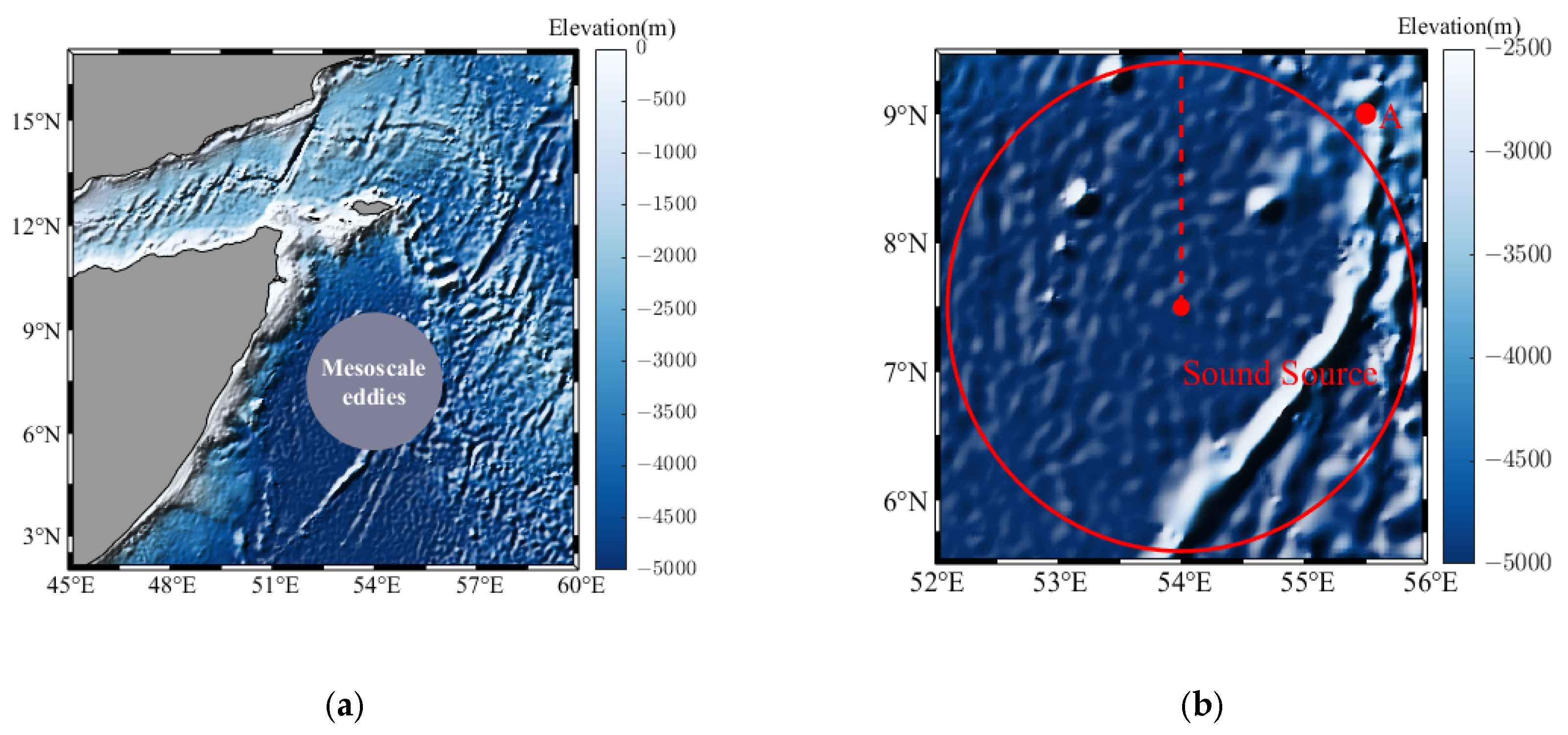
This study employs the BELLHOP acoustic model to systematically investigate the mechanisms of acoustic propagation variability under the combined influence of mesoscale eddies and rough sea surfaces. The objective is to elucidate how these multiphysical processes jointly affect underwater sound propagation. The experimental domain is centered on the core of a mesoscale eddy located at 7.5°N, 54°E. A circular computational domain with a radius of 200 km is established around this location (Figure 2a).

The seafloor topography in the region is relatively flat, with an average water depth of approximately 5303 m. This minimizes the influence of bathymetric scattering on acoustic propagation. Detailed model parameter settings are summarized in

Table 1. Key parameter matrix for underwater sound propagation.

Parameter	Value	Physical Implication
Source Frequency	1 kHz	high frequency sound wave
Source Depths	10/200/800 m	Surface duct/Convergence zone/Deep convergence zone
Bottom Density	1.3 g/cm3	Sandy sediment characteristics
Bottom Sound Speed	1600 m/s	Geoacoustic inversion results
Attenuation Coefficient	0.6 dB/λ	High-frequency scattering loss

.

The source frequency was set to 1 kHz, which corresponds to typical operational frequencies used by submarines and surface vessels [40]. The bottom sediment density was assigned a value of 1.3 g/cm³, following the deep-sea sediment acoustic parameters reported by Wang [41], representing sandy sediment characteristics commonly found in abyssal environments [42]. The bottom sound speed was set to 1600 m/s, and the attenuation coefficient was specified as 0.6 dB/λ. These values reflect high-frequency scattering losses typically observed in such deep-water environments.

In this study, the 54°E meridian (indicated by the dashed line in Figure 2b) is selected as the cross-section for analyzing acoustic propagation characteristics due to its alignment with the mesoscale eddy core. A three-layer sound source deployment scheme is implemented to investigate the response mechanisms at different depths: 10 m depth to represent surface duct propagation, 200 m depth to examine the formation mechanisms of convergence zones, and 800 m depth to analyze deep convergence zone structures and their propagation characteristics [43].

The experimental design includes four comparative scenarios (

Table 2. Set-up of the four sound propagation experiments.

Sub-Experiment	With Eddy	With Rough Sea Surface	Purpose
Baseline	F	F	Reference for the following experiments
Pure eddy	T	F	Study the effect of eddy only without rough sea surface
Pure roughness	F	T	Study the effect of rough sea surface only without eddy
Couple	T	T	Study the effect of eddy coupled with rough sea surface

):

1. Baseline scenario: a static sea surface and homogeneous water body.

2. Pure eddy scenario: retains only the mesoscale eddy’s temperature and salinity structures.

3. Pure roughness scenario: combines a wind-wave field described by the PM spectrum with a flat-bottom topography.

4. Fully coupled scenario: joint effects of mesoscale eddies and rough sea surfaces.

Using stratified comparisons, this study quantitatively examines three mechanisms:

1. How mesoscale eddy-induced sound speed anomalies affect the reconstruction of convergence zones.

2. How rough sea surfaces influence near-field scattering losses.

3. The nonlinear coupling effects of multi-scale marine environmental factors.

4.1. Experiment 1: Baseline Scenario

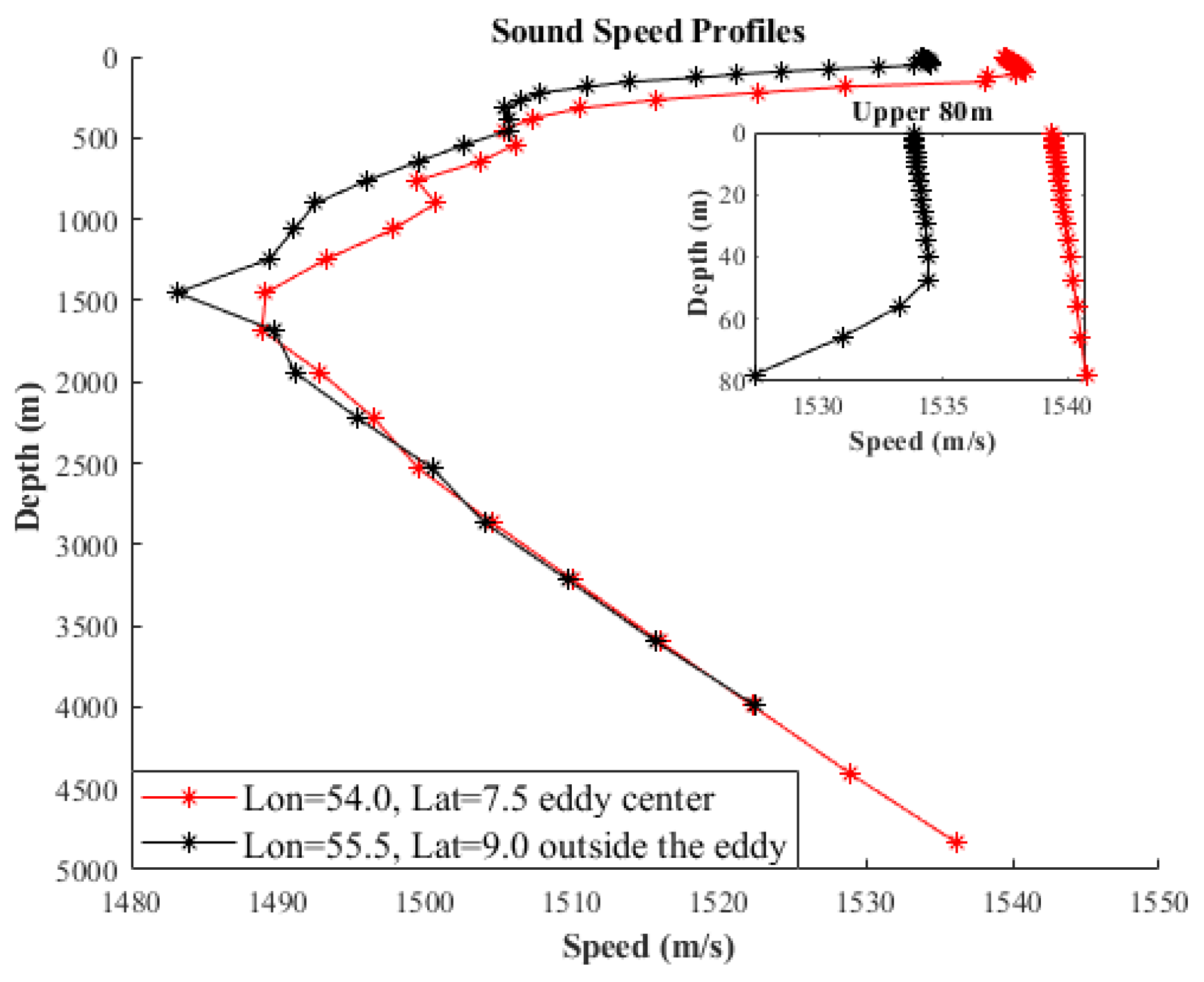
In Experiment 1, the background sound speed profile was derived from temperature and salinity data at Point A (55.5°E, 9°N) in Figure 2b. This location lies outside the influence of mesoscale eddies and serves as an appropriate baseline scenario. The sound speed profile was computed using an empirical formula based on CMEMS reanalysis data. Due to the layered structure inherent in reanalysis products, the resulting sound speed profile exhibited limited vertical smoothness. Nevertheless, it represents typical oceanographic conditions in the study area and was used as the reference for acoustic modeling. To ensure a simplified and idealized propagation environment, neither mesoscale eddies nor sea surface roughness effects were included in this experiment. The derived sound speed profile was directly input into the BELLHOP model without further modification. 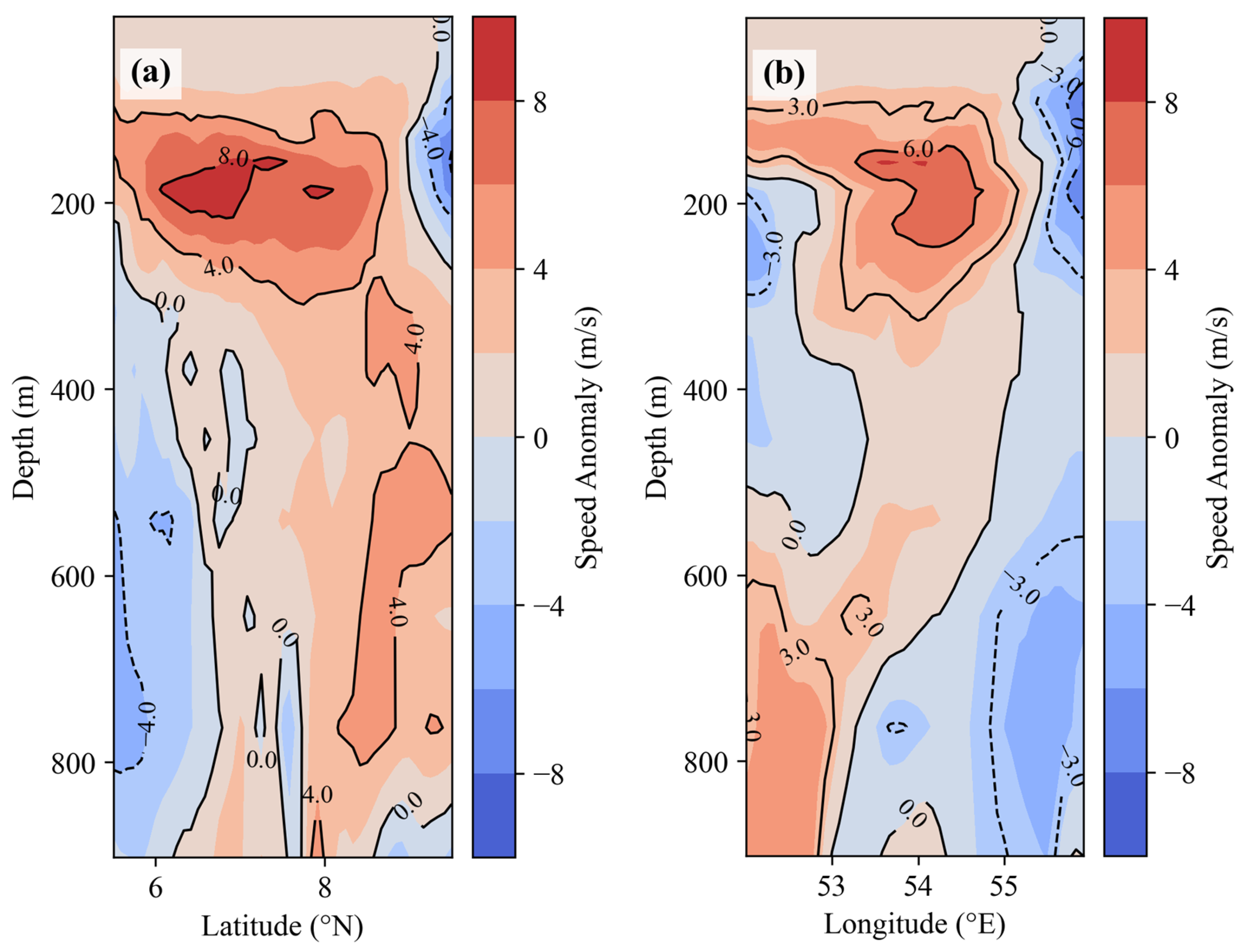For comparative analysis, Figure 9 illustrates the differences between this background profile and the sound speed anomaly observed at the eddy center.

Figure 10 illustrates the transmission loss associated with three distinct acoustic propagation modes, surface duct propagation, convergence zone propagation, and deep convergence zone propagation, along the northward direction (indicated by the red dashed line) from the sound source shown in Figure 2b.

When the sound source is positioned at a depth of 10 m, a clear surface duct is observed, characterized by low transmission loss due to the confinement of acoustic energy near the sea surface. With the source located at 200 m depth, three distinct convergence zones emerge within the 200 km propagation range. These zones reflect the focusing of sound energy at specific intervals, resulting from interactions between the acoustic field and the mesoscale eddy’s sound speed structure.

As illustrated in Figure 10, the sound rays are distributed across the entire propagation domain, undergoing complex interactions with both the rough sea surface and the thermohaline structure of the mesoscale eddy. These interactions demonstrate the significant modulation effects of the marine environment on acoustic propagation and provide a basis for further analysis of multiphysical coupling mechanisms.

4.2. Experiment 2: Pure Eddy Scenario

In this sub-experiment, the influence of mesoscale eddies on the sound speed field is examined in isolation. The distribution of sound speed anomalies in the vertical cross-section aligns with the spatial pattern presented in Figure 9. To facilitate a more intuitive understanding of how acoustic transmission loss varies with propagation distance, one-dimensional transmission loss curves are provided for each source depth (Figure 11). These curves illustrate the modulation effects of mesoscale eddy-induced sound speed anomalies on acoustic propagation, offering insights into the interaction between oceanic dynamics and underwater acoustics.

In Figure 11, Sz denotes the source depth, and Rz denotes the receiver depth.

Figure 11a compares the transmission loss characteristics under the influence of a mesoscale eddy with those in the baseline (non-eddy) environment. When both the sound source and receiver are located at a depth of 10 m, the transmission loss curve exhibits periodic fluctuations (red curve), caused by perturbations in the sound speed profile induced by the warm eddy. The amplitude of these fluctuations increases by approximately 5 dB compared to the baseline scenario (black curve). This oscillatory behavior results from phase interference among sound wave propagation paths that have been altered by the eddy-induced sound speed anomaly. Notably, when the propagation distance exceeds 150 km, the transmission loss under the eddy’s influence decreases by about 3–5 dB relative to the baseline, suggesting a potential enhancement of the waveguide effect at this spatial scale.

When both the sound source and receiver are positioned at a depth of 200 m, the first, second, and third convergence zones shift forward by approximately 4 km, 10 km, and 17 km, respectively, under the influence of the mesoscale eddy. In addition, the peak energy levels in the first and second convergence zones decrease by about 6 dB compared to the baseline. However, in non-convergence regions, the transmission loss under eddy conditions is slightly lower than that observed in the baseline case. To investigate this phenomenon, the corresponding ray tracing diagram is presented in Figure 12. Black represents sound rays that are in contact with both the sea surface and the seabed, red represents sound rays that are not in contact with either, and green represents sound rays that are in contact with only the sea surface. Compared to the baseline scenario, the presence of the warm eddy results in a steeper sound speed gradient, leading to a smaller curvature radius of the limiting rays. This causes the convergence zone positions to shift forward and the turning depth of the rays to increase, thereby reducing the number of dominant rays carrying most of the acoustic energy. Consequently, the transmission loss within the convergence zones increases.

Some rays reflect without reaching the seafloor and subsequently reverse direction, returning toward the sea surface and entering the shadow zone. This ray leakage into the shadow region results in slightly reduced transmission loss compared to the baseline case.

When both the sound source and receiver are positioned at a depth of 800 m, the convergence zones exhibit a forward shift due to the influence of the mesoscale eddy. Additionally, the number of convergence zones increases, though their distinctiveness diminishes. This behavior arises from the same mechanisms previously discussed: the alteration of the sound speed gradient and the reduced curvature radius of the limiting rays. These factors collectively modify the convergence patterns and energy distribution within the deep sound channel. These observations highlight the intricate interplay between mesoscale eddies and acoustic propagation in deep-sea environments, emphasizing the sensitivity of the deep sound channel to thermohaline variability induced by mesoscale features.

4.3. Experiment 3: Pure Rough Sea Surface Scenario

In this experiment, the hydrological environment is kept consistent with the baseline scenario to maintain an identical sound speed field, allowing a focused analysis of the impact of rough sea surfaces on acoustic propagation. A schematic of the rough sea surface (partial view) is shown in Figure 7. In the BELLHOP model, the sea surface height is updated every 0.25 km. The simulation results for Experiment 1 (baseline) and Experiment 3 (rough sea surface) are presented in Figure 13.

Figure 13a illustrates the transmission loss for a sound source at a depth of 10 m, excluding the effects of eddies or rough sea surfaces. Figure 13b shows the transmission loss when only the influence of rough sea surfaces is considered. To better visualize the variation in acoustic transmission loss with distance, one-dimensional transmission loss curves for the 10 m sound source depth are provided in Figure 14.

When sound waves interact with the sea surface, they obey Snell’s law of refraction. Within the surface duct, continuous refraction due to the sound speed gradient confines acoustic energy, resulting in significant energy accumulation in convergence zones. However, a rough sea surface disrupts this interaction by altering the incident angles of the sound rays. According to Snell’s law, small changes in the incident angle lead to substantial shifts in the refraction angle. As a result, some rays escape the surface duct due to increased refraction angles, demonstrating the modulating effect of sea surface roughness on acoustic propagation.

Assuming the ray’s launch angle is ${\theta }_i$, the sound speed at the source location is $c_i$, and the ray’s turning angle at the lower boundary of the surface duct is ${\theta }_t$ = 0° with the sound speed at the lower boundary being ${\mathrm{c}}_t$, Snell’s law of refraction $\cos {\theta }_i/c_i$ = $\cos {\theta }_t/c_t$ yields $\cos {\theta }_i$ = $c_i\cos {\theta }_t/c_t$, which defines the critical angle ${\theta }_{ic}=\arccos (c_i/c_t)$ at which the ray turns. Therefore, rays with launch angles within $\pm |\arccos (c_i/c_t)|$ interact only with the sea surface and propagate within the surface duct. As the grazing angle increases, the rays no longer turn upward but instead turn downward, becoming rays that no longer interact with the sea surface. When the grazing angle continues to increase, the rays escape the surface duct and follow the convergence zone propagation pattern.

This process reduces the energy density within the surface duct and diminishes the sound intensity distribution in the far-field convergence zones. The ‘escaped’ rays enhance the characteristics of the convergence zones, resulting in peak energy levels nearly identical to those in Experiment 1. However, in the shadow zone, the rough sea surface causes an energy difference of approximately 20 dB. These findings highlight the significant impact of sea surface roughness on acoustic propagation, particularly in altering the energy distribution across the surface duct, convergence zones, and shadow zones.

Figure 15 shows the relationship between distance and transmission loss when the sound source is placed at depths of 200 m and 800 m, with only the influence of rough sea surfaces considered. The results demonstrate strong agreement between both scenarios, suggesting that the impact of rough sea surfaces on convergence zone propagation and deep sound channel propagation is minimal. This indicates that the primary effects of sea surface roughness are limited to near-surface acoustic propagation, while deeper propagation modes remain largely unaffected.

4.4. Experiment 4: Coupled Rough Sea Surface and Eddy Scenario

In this experiment, the sound speed field is derived from CMEMS hydrological data combined with empirical formulas, while the upper boundary for acoustic propagation is established using the SWAN wave model to generate the wave spectrum for the target area, integrated with the Monte Carlo method to simulate a realistic and complex marine environment. Acoustic propagation analysis is performed using the sound speed field and rough sea surface conditions at 00:00 UTC on 31 July. For comparative analysis, transmission loss curves at various depths are presented in Figure 16. The black curve represents Experiment 1 (baseline), the red curve represents Experiment 2 (pure eddy), the blue curve represents Experiment 3 (pure rough sea surface), and the green curve represents Experiment 4 (coupled rough sea surface and eddy).

As shown in the figures, when the sound source is positioned at a depth of 10 m, the acoustic energy is primarily confined within the surface duct. The propagation loss is mainly influenced by the rough sea surface, while the presence of the eddy slightly reduces the propagation loss and weakens the convergence zone characteristics. This is likely because the eddy expands the depth of the surface duct, reducing the escape of sound rays and thereby increasing the acoustic energy compared to the scenario with only rough sea surfaces.

When the sound source is set at depths of 200 m and 800 m, the blue and black curves show good agreement, indicating that the rough sea surface has a minimal impact on acoustic propagation at these depths. The presence of the eddy causes the convergence zones to shift forward and reduces their peak energy, consistent with the findings in Experiment 2. When both rough sea surfaces and eddies are considered, the green and red curves exhibit good agreement, suggesting that the eddy dominates the propagation loss. Additionally, the rough sea surface stabilizes the acoustic energy, reducing fluctuations in propagation loss.

The conclusions drawn from these three scenarios are relatively general and do not clearly distinguish the boundary depth at which rough sea surfaces or eddies play a dominant role. Therefore, a supplementary experiment was designed. Considering that the influence of rough sea surfaces is closely related to the surface duct, Figure 9 shows that the sound speed in Experiment 1 exhibits a positive gradient above 40 m and a negative gradient below 40 m. Under eddy influence, the sound speed profile maintains a positive gradient up to 80 m. Thus, the sound source in the supplementary experiment was set at a depth of 40 m. In Experiment 1, the sound rays follow the convergence zone propagation pattern, while in Experiment 2, they still adhere to the surface duct propagation rules. The resulting one-dimensional propagation loss plot is shown in Figure 17.

In Experiment 1 (baseline), represented by the black curve, sound rays are not confined to the surface duct, resulting in distinct convergence zones and shadow zones.

In Experiment 2 (pure eddy), shown by the red curve, the elevated sea surface temperature expands the surface duct, confining most acoustic energy within it. Consequently, sound ray fluctuations are relatively smooth, with a gradual decrease in transmission loss over distance. Compared to the baseline, the transmission loss exhibits significant differences.

In Experiment 3 (pure rough sea surface), depicted by the blue curve, prominent convergence zones and shadow zones persist. However, the convergence zones shift forward by approximately 5 km compared to Experiment 1, while peak energy levels remain unchanged. This shift may result from excessive refraction of sound rays caused by the rough sea surface, indicating that rough sea surfaces affect not only propagation mechanisms within the surface duct but also sound rays in shallow water following the convergence zone propagation pattern.

In Experiment 4 (coupled rough sea surface and eddy), represented by the green curve, the overall acoustic energy increases compared to Experiment 3, but the convergence zone characteristics are weakened. This aligns with the earlier explanation that a warm eddy expands the surface duct, concentrating acoustic energy. The notable difference between the red and green curves stems from the rough sea surface disrupting the surface duct, causing sound rays to “escape” and reducing the energy in the green curve. Compared to the black curve, the blue curve shows a partial forward shift, suggesting that when the sound source is in shallow water and follows the convergence zone propagation pattern, rough sea surfaces have a measurable but significantly smaller impact than on the surface duct.

5. Conclusions

This study systematically elucidates the synergistic regulation of mesoscale eddies and rough sea surfaces on acoustic propagation in the Gulf of Aden during summer, using a SWAN–BELLHOP multiphysics coupling model validated against Jason-3 satellite altimetry data to ensure the accuracy of SWAN simulations. Key findings reveal that rough sea surfaces significantly increase near-field transmission loss in the surface duct (10 m depth) by approximately 20 dB compared to an ideal smooth sea surface, while mesoscale eddies deepen the surface duct from 40 m to 80 m, reducing acoustic energy leakage and modulating convergence zone characteristics. At the transition depth (40 m), rough sea surfaces cause the first convergence zone to shift forward by approximately 5 km without altering peak sound intensity, whereas mesoscale eddies enhance the trapping efficiency of the surface duct, re-confining escaped sound rays and offering insights for optimizing shallow-water sonar performance. In deep-water propagation (≥200 m), mesoscale eddies dominate, with warm eddies (Δc = 8.3 m/s) shifting convergence zones forward and reducing peak sound intensity by approximately 10 dB, while rough sea surfaces have a negligible impact. The multiscale coupling model of mesoscale eddies, rough sea surfaces, and acoustic propagation overcomes the limitations of traditional single-factor methods by incorporating SWAN-simulated wave spectra in place of the classical PM spectrum, enhancing the reliability of acoustic propagation predictions under complex sea conditions. These findings provide critical theoretical support for underwater target detection and acoustic communication system optimization in the Gulf of Aden, with direct applications in sonar array deployment depth selection and dynamic convergence zone correction.