Abstract
Satellite cloud images exhibit complex multidimensional characteristics, including spectral, textural, and spatiotemporal dynamics. The temporal evolution of cloud systems plays a crucial role in accurate classification, particularly under the coexistence of multiple weather systems. However, most existing models—such as those based on convolutional neural networks (CNNs), Transformer architectures, and their variants like Swin Transformer—primarily focus on spatial modeling of static images and do not explicitly incorporate temporal information, thereby limiting their ability to effectively integrate spatiotemporal features. To address this limitation, we propose SIG-ShapeFormer, a novel classification model specifically designed for satellite cloud images with temporal continuity. To the best of our knowledge, this work is the first to transform satellite cloud data into multivariate time series and introduce a unified framework for multi-scale and multimodal feature fusion. SIG-Shapeformer consists of three core components: (1) a Shapelet-based module that captures discriminative and interpretable local temporal patterns; (2) a multi-scale Inception module combining 1D convolutions and Transformer encoders to extract temporal features across different scales; and (3) a differentially enhanced Gramian Angular Summation Field (GASF) module that converts time series into 2D texture representations, significantly improving the recognition of cloud internal structures. Experimental results demonstrate that SIG-ShapeFormer achieves a classification accuracy of 99.36% on the LSCIDMR-S dataset, outperforming the original ShapeFormer by 2.2% and outperforming other CNN- or Transformer-based models. Moreover, the model exhibits strong generalization performance on the UCM remote sensing dataset and several benchmark tasks from the UEA time-series archive. SIG-Shapeformer is particularly suitable for remote sensing applications involving continuous temporal sequences, such as extreme weather warnings and dynamic cloud system monitoring. However, it relies on temporally coherent input data and may perform suboptimally when applied to datasets with limited or irregular temporal resolution.
1. Introduction
Clouds play a central role in regulating the radiation budget, water cycle, and biogeochemical processes on Earth, thereby exerting a profound influence on global climate change [1]. According to data from the International Satellite Cloud Climatology Project (ISCCP), the global annual average cloud cover accounts for approximately two thirds of the total surface area of Earth [2]. Accurate identification of cloud types and their dynamic distribution patterns is important for fine-scale meteorological forecasting, weather modification operations, and disaster early warning [3,4]. Cloud classification, as a type of remote sensing scene classification, has become a fundamental task aimed at classifying remote sensing images into predefined semantic categories utilizing spatial and spectral information from the images [5]. This study constructs a classification system based on satellite cloud images, covering 11 meteorological categories, which encompass weather systems, cloud systems, and terrestrial systems.
Early studies were dominated by threshold methods, which segmented cloud features by setting spectral or brightness temperature thresholds. For example, Yang Cheng et al. [6] used a multi-spectral threshold method to classify GMS-5 satellite data, creating a three-level system for high, medium, and low clouds; Zhou Xuejun et al. [7] proposed a threshold method based on grayscale characteristics, using mean and variance statistics to differentiate between clear, thick, and thin cloud regions. With technological development, statistical methods have gradually been applied to cloud classification research, with typical methods including maximum likelihood and clustering analysis. Li et al. [8] combined spectral-spatial features from MODIS data to classify cloud systems using maximum likelihood; Wu Yongming et al. [9] introduced fuzzy C-means clustering (FCM) to improve the classification of edge cloud systems through membership degree calculations.
In recent years, machine learning methods have made significant progress in cloud classification. Li et al. [10] proposed a feature representation method for ground-based cloud images based on a bag of micro-structures and combined it with Support Vector Machine (SVM) technology to classify the cloud images into five categories; Yu et al. [11] used the random forest (RF) algorithm to classify FY-4A satellite data into 8 categories of single-layer clouds and 12 categories of multilayer clouds, with an accuracy of 70% for single-layer clouds; Tan et al. [12] developed a multilayer cloud detection model using Himawari-8 satellite data for all-weather cloud classification; Zhang et al. [13] constructed a random forest classification framework by combining the cloud product CloudSat 2B-CLDCLASS and Himawari-8 multichannel data.
Meanwhile, deep learning technologies have demonstrated stronger feature learning capabilities. CNN-based approaches have demonstrated remarkable capabilities in spatial feature extraction for cloud classification. Wang et al. [14] pioneered a CNN-LSTM hybrid architecture that leverages convolutional layers to capture spatial patterns while using LSTM to model temporal evolution. Subsequent innovations include a lightweight CloudNet optimized for cloud feature representation by Zhang et al. [15] and a task-driven T-GCN proposed by Liu et al. [16] that outperforms conventional CNNs in edge cloud classification through graph convolutions. DeepCTC by Afzali et al. [17] further advanced this direction with 85% accuracy in multi-class cloud categorization. Temporal modeling techniques address these limitations through specialized architectures for sequence analysis. The Shapelet method has been widely applied in various domains, including extreme weather classification and segment recognition, fault diagnosis, physiological signal classification, and hyperspectral image classification [18,19,20,21,22], demonstrating its effectiveness in capturing discriminative subsequences within time-series data. In recent years, Transformer-based methods have achieved significant progress in remote sensing image classification and segmentation. For instance, STMSF enhances the representational capacity of the Swin Transformer for multi-scale objects in remote sensing imagery through a multi-scale feature fusion mechanism [23,24,25]. Models such as RSPrompter and DynamicVis incorporate dynamic prompts and conditional attention mechanisms, thereby improving adaptability to complex remote sensing scenes [26,27]. Moreover, Mamba, an emerging sequence modeling framework, has demonstrated unique advantages in the domain of remote sensing image analysis. In high-resolution remote sensing image processing, Mamba not only improves global context modeling capabilities but also significantly reduces computational costs while maintaining high accuracy [28]. This makes Mamba a powerful tool for handling large-scale remote sensing data, particularly in complex scenarios involving multi-scale object recognition [29]. Furthermore, leveraging continuous-state space models, Mamba efficiently processes long sequences and avoids the quadratic complexity associated with traditional attention mechanisms [30].
In recent years, despite significant advances in deep learning for cloud image feature extraction and model architectures, existing approaches still face three critical challenges [31,32]. First, most existing approaches, such as CNN or GCN-based models, primarily focus on extracting spatial features from static images, often treating satellite cloud images as independent frames [33]. This approach overlooks the temporal evolution characteristics inherent to cloud systems. Second, many current deep learning-based cloud image classification models still operate as “black-box” systems, which significantly limits their reliability and practical applicability in operational settings. Third, although temporal modeling approaches such as Transformers demonstrate strong capabilities in capturing the long-term dynamics of cloud systems, they often struggle to extract fine-grained spatial features due to weak local perception mechanisms. Moreover, such methods typically focus only on temporal variations, failing to effectively integrate complementary modalities such as spatial textures and morphological structures. In contrast, our work highlights the importance of combining diverse and complementary features through an adaptive multimodal fusion framework to achieve more robust and interpretable classification.
To mitigate and address these challenges, this study proposes an innovative classification model named SIG-ShapeFormer, designed for efficient intelligent recognition of cloud systems under dynamic temporal variations in high-resolution satellite cloud imagery. (1) To alleviate the static spatial modeling limitation, we transform satellite cloud images into multivariate time series and develop a multi-scale Inception module integrated with Transformer encoding to jointly capture both local textures and global temporal dynamics. (2) For improving interpretability, we employ Shapelet-based feature extraction to identify physically meaningful subsequences that reveal discriminative cloud evolution patterns, thereby enhancing model transparency. (3) To resolve the spatial-temporal imbalance issue, we propose a differential-enhanced GASF transformation to encode fine-grained structural features while the designed EAFM module adaptively fuses morphological, temporal, and spatial features through attention mechanisms to ensure complementary multimodal learning. These innovations collectively improve classification accuracy while maintaining interpretability and robustness.
The main contributions of this paper are summarized as follows:
- We propose a novel satellite cloud image classification framework, SIG-ShapeFormer, which independently extracts shape, spatial, and temporal features from cloud images and effectively fuses them through an EAFM (Ensemble-Attention Feature Mixer) block, thereby enhancing the classification accuracy across diverse cloud types;
- We develop a multi-scale feature extraction architecture based on the Inception framework, which integrates parallel 1D convolutional branches with varying kernel sizes (from 1 × 1 to 1 × 7) to construct a multi-level feature pyramid, enabling the model to simultaneously capture both local texture details and global temporal sequence features in cloud systems;
- We design a differential-enhanced GASF transformation module that combines first-order and second-order difference information to convert time-series cloud data into spatially meaningful 2D representations, significantly improving the ability of the model to characterize cloud boundaries and internal structures;
- The proposed SIG-ShapeFormer model demonstrates outstanding classification performance, achieving 99.36% accuracy on the LSCIDMR-S dataset, a significant improvement over the original ShapeFormer model. Additionally, it achieves higher accuracy on 6 out of 8 datasets from the UCM remote sensing dataset and the UEA archive dataset, showcasing robust generalization capabilities across diverse meteorological conditions.
2. Data
2.1. Original Data Description
This study employs the LSCIDMR satellite cloud image database [34], the first large-scale benchmark dataset specifically designed for meteorological research, derived from observations by the Himawari-8 geostationary meteorological satellite launched by Japan. The dataset comprises 104,390 preprocessed RGB images (256 × 256 pixels) with 10-min temporal resolution and 2-km spatial resolution covering the Northern Hemisphere, synthesized from three spectral bands: albedo_5, albedo_4, and albedo_3. The images are categorized into three meteorologically significant systems (weather, cloud, and surface systems) with 10 subclasses and an additional “PatchElse” unlabeled category. Each image follows the naming convention YYYYMMDD_ii_jj.png, where ii and jj denote latitude and longitude slice indices, respectively. The dataset is publicly available at https://github.com/Zjut-MultimediaPlus/LSCIDMR, accessed on 25 December 2024.
To evaluate the generalization ability of our model, we conducted experiments on seven multivariate time-series datasets from the UEA archive and the UCMerced Land Use Dataset (referred to as the UCM dataset). The UEA archive, maintained by the University of East Anglia, is a widely recognized benchmark for multivariate time-series classification. It contains datasets spanning various domains such as healthcare, activity recognition, and environmental monitoring, thereby ensuring diversity and broad applicability. Meanwhile, the UCM dataset is a benchmark dataset in remote sensing image analysis, featuring high-resolution aerial imagery with a spatial resolution of 0.3 m. It comprises 21 scene categories, each containing 100 images, and has been extensively utilized for land cover classification and computer vision research. Since the UCM dataset does not include temporal information, we applied a specific preprocessing strategy: each image was first segmented, and then the segmented patches were stacked to form a sequence that reflects spatial variation patterns. This approach compensates for the lack of temporal features in UCM and provides our model with abundant spatial feature information, thus enhancing its applicability across heterogeneous datasets. The specific details of the remote sensing datasets and UEA datasets used in this study are presented in Table 1.

Table 1.
Details of the remote sensing and UEA datasets used in this study.
The LSCIDMR provides two annotation formats: single-label (LSCIDMR-S, 40,625 samples) and multi-label (LSCIDMR-M, 414,221 samples). In this work, we employ the single-label subset (LSCIDMR-S), where annotations are manually verified by meteorological experts to ensure reliability (representative examples shown in Figure 1).
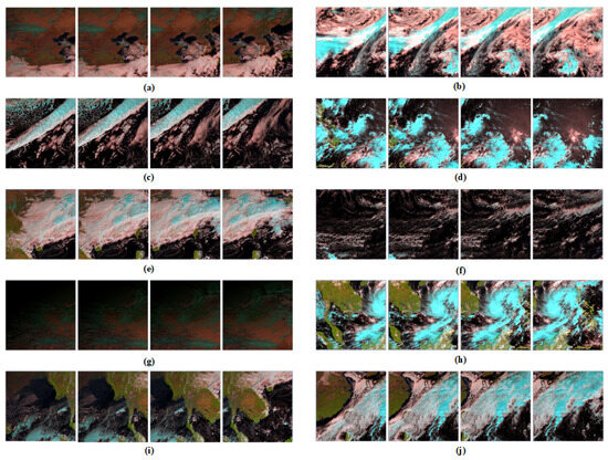
Figure 1.
Examples of ten categories in the LSCIDMR-s dataset: (a) Desert, (b) Extratropical Cyclone, (c) Frontal Surface, (d) High-Ice Cloud, (e) Low-Water Cloud, (f) Ocean, (g) Snow, (h) Tropical Cyclone, (i) Vegetation, (j) Westerly Jet.
To address the significant class imbalance in the LSCIDMR-S dataset (Table 2), where non-informative samples (PatchElse) account for 60% of data while critical meteorological categories like westerly jets represent less than 1%, we developed a spatiotemporal sampling strategy. Leveraging image spatiotemporal tags (YYYYMMDD_ii_jj.png), we implemented a hybrid sampling rule combining “fixed coordinate positions + continuous temporal sequences” with manual curation to ensure spatiotemporal continuity for rare categories. This approach ultimately yielded a balanced subset of 5000 images for model training and evaluation, significantly enhancing the reliability of performance assessment.
Table 2.
Proportions of Cloud Image Categories in the LSCIDMR-S Dataset.
2.2. Data Preprocessing
The dynamic evolution of meteorological systems (e.g., typhoon movement, frontal progression) manifests itself as continuous temporal variations in satellite cloud imagery. Conventional spatial convolution-based models, limited by their lack of temporal modeling capability, struggle to capture such long-range dependencies. In contrast, time-series analysis methods effectively model dynamic evolution patterns by analyzing features such as cloud morphology and movement velocity. As shown in Figure 2, the two categories of satellite cloud images exhibit distinct spatial variation patterns under the same temporal resolution.
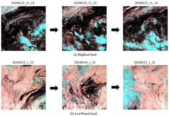
Figure 2.
The dynamic changes and evolution process of spatial information observed in satellite cloud images of the same category.
Studies show that satellite cloud imagery exhibits intra-class temporal consistency and inter-class temporal divergence: sequential images of the same weather type follow regular temporal evolution, while temporal evolution patterns differ significantly across weather systems.
This study innovatively proposes a spatiotemporally decoupled multivariate time-series (MTS) transformation framework (as illustrated in Figure 3), which converts raw satellite cloud imagery into meteorologically meaningful multivariate time-series data through a three-stage processing architecture:

Figure 3.
Systematic Conversion Process from Satellite Cloud Image Data to Multivariate Time-Series (MTS) Data.
Spatial Partitioning and Local Feature Encoding. The 5000 high-resolution satellite cloud images are uniformly partitioned using a grid strategy, generating 16 local regions (each pixels). Each region is flattened into a one-dimensional feature vector in row-major order [35], encoding local characteristics such as cloud reflectance distribution and textural structures (denoted as num_features). This process discretizes 2D image features into a high-dimensional vector space, providing primitives for subsequent temporal modeling.
Global Trend Preservation and Dimensionality Reduction. To mitigate high-dimensional redundancy, Global Average Pooling (GAP) is applied to the 16 local vectors. This operation preserves the global reflectance trends of the full image while compressing the feature dimensions from to 4096, significantly reducing computational complexity.
Temporal Alignment and Data Standardization. Based on the continuity of meteorological events, the pooled feature sequences are grouped and temporally aligned according to weather type labels. The alignment length T is defined as half the difference between the maximum and minimum continuous sequence lengths. The final output is a multidimensional time series , where 4096 denotes the feature dimension (num_features), and 13 represents the unified time-step length (time_steps). The linear interpolation-truncation hybrid strategy is adopted to normalize sequence lengths: Sequences shorter than the alignment length T are extended to T via linear interpolation, ensuring temporal continuity. Sequences exceeding T are truncated to the first T time slices, preserving critical information from the initial evolutionary phases.
This approach guarantees consistent data length while balancing computational efficiency and the retention of meteorological event characteristics (the complete workflow is illustrated in Figure 3).
3. Methods
3.1. Problem Formulation and Overall Model Structure
Similar to previous studies, we define the satellite cloud image classification task as a multimodal spatiotemporal feature fusion problem. The input data to the model is , a sequence of preprocessed satellite cloud images (see Section 2 for data preprocessing). Each represents a multivariate time-series format. The variable denotes the classification result among 11 predefined cloud image categories.
Specifically, our SIG-ShapeFormer model processes the input through three parallel channels: a Shapelet-based feature extraction channel (S-channel), a multi-scale Inception-based temporal channel (I-channel), and a GASF (Gramian Angular Summation Field) transformation-based spatial channel (G-channel). These three channels extract shape features , temporal features , and spatial features , respectively.
The extracted features are concatenated and passed through the designed EAFM module (Ensemble-Attention Feature Mixer) for adaptive fusion, ultimately resulting in the prediction of the model . The overall classification process can be expressed as:
where EAFM(·) denotes the proposed multimodal fusion module combining attention mechanisms and ensemble learning, and SIG(·) represents the three feature extraction channels of the model.
Figure 4 illustrates the Trichannel architecture with EAFM Block. In the subsequent Section 3.2, Section 3.3, Section 3.4 and Section 3.5, we will provide detailed introductions to each of these components.
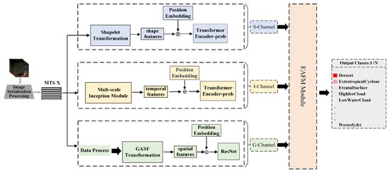
Figure 4.
Overall Architecture of the SIG-ShapeFormer Model, S-Channel:A feature extraction channel based on Shapelet techniques; I-Channel: A feature extraction channel utilizing multi-scale Inception modules; G-Channel: A feature extraction channel based on GASF transformation; EAFM Block: A multimodal feature fusion channel integrating ensemble learning and attention mechanisms.
Inspired by ShapeFormer, our SIG-ShapeFormer introduces a differential-enhanced GASF transformation channel to optimize the capability of capturing spatial information. To simultaneously extract both local and global features from satellite cloud image sequences, we propose a multi-scale Inception module, enhancing feature learning beyond the generic feature extraction module in the original ShapeFormer. This approach facilitates joint extraction of local and global features. To achieve efficient and adaptive fusion of multimodal features and address their inherent heterogeneity, we design an Ensemble-Attention Feature Mixer (EAFM) module, which integrates the concept of stacking learning from ensemble learning with attention mechanisms to achieve dynamic feature fusion. This approach significantly enhances the accuracy and robustness of predictions.
Table 3 provides a detailed overview of the core workflow, main modules, and processing channels of the SIG-ShapeFormer model, with bolded components highlighting key improvements over the original ShapeFormer architecture. As shown in Table 3, the proposed model consists of three primary channels, S-channel, I-channel, and G-channel, that perform feature extraction and preliminary classification, as described in Section 3.2, Section 3.3 and Section 3.4. These features are then fused using the EAFM module, an Ensemble-Attention Feature Mixer inspired by the stacking strategy in ensemble learning and enhanced with attention mechanisms. The fused feature representation is subsequently passed to a metaclassifier (composed primarily of linear mapping and softmax) to generate the final prediction, detailed in Section 3.5. To further clarify the flow of the features and the intermediate representations within the model, Table 4 provides a summary of all the variables used, along with their definitions.
Table 3.
Processing Stages and Corresponding Operations of the Shapeformer Model, with Bolded Components Highlighting Key Improvements over the Original Architecture.
Table 4.
Notation Table of Mathematical Symbols and Terms Used in SIG-ShapeFormer.
3.2. Shapelet-Based Feature Extraction Channel (S-Channel)
Satellite cloud images exhibit the intra-class temporal consistency characteristic, where consecutive images of the same weather type follow regular dynamic evolution over time. Leveraging this property, we propose a Shapelet-based feature classifier to extract category-discriminative local spatiotemporal patterns from cloud image time series. The Shapelet extraction module builds upon the implementation from the OSD (Offline Shapelet Discovery) method in the ShapeFormer model [36]. As shown in Figure 5, the workflow of the S-channel encompasses three critical stages: Shapelet Transformation (see Section 3.2.1), while temporal modeling and classification handle global perception and analysis of the differential features (see Section 3.2.2).
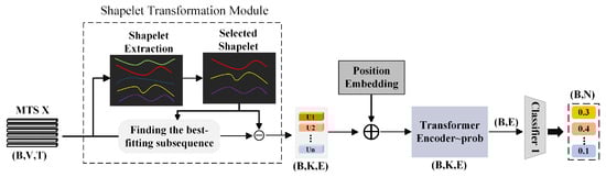
Figure 5.
Overview of the Workflow for the Shapelet-based Feature Extraction Channel (S-Channel).
3.2.1. Shapelet Transformation
In the task of satellite cloud image classification, Shapelets are defined as discriminative subsequences that characterize the key dynamic patterns of specific weather categories. These subsequences enable effective class discrimination by capturing significant variations in local spatiotemporal features. Given a multivariate time series (MTS) converted from satellite cloud images, where B denotes the batch size, V the feature dimensionality, and T the unified time steps, this study employs the Offline Shapelet Discovery (OSD) method [36]. The core workflow of OSD consists of two stages: Shapelet extraction and selection. The detailed process is illustrated in Figure 6.
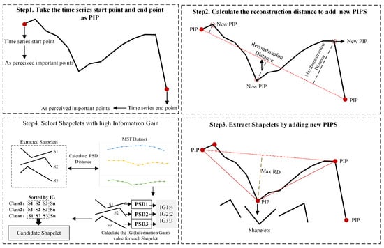
Figure 6.
Detailed Explanation of the Shapelet Extraction and Selection Process.
As illustrated in Steps 1 to 3 of Figure 6, the process of Shapelet extraction is carried out. In this stage, the Perceived Important Points (PIP) detection technique is employed to iteratively select time points that maximize the reconstruction distance, beginning with the first and last points of the sequence. The reconstruction distance is defined as the perpendicular distance from a candidate point to the line segment formed by its two nearest previously selected important points. By constructing a set of three consecutive PIPs—typically amounting to 20% of the total sequence length—at least one Shapelet subsequence can be generated. For each Shapelet, its value vector, start and end indices, and associated class label are recorded. This process yields multiple candidate Shapelets per class for subsequent selection. This paper selected cloud image data from the LSCIDMR-S dataset that represents three distinct weather systems, forming a multivariate time series. Shapelet extraction and selection were then performed on these sequences. For each time series, the three most representative Shapelets were retained, as shown in Figure 7.
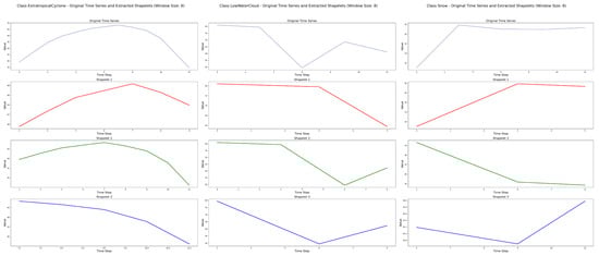
Figure 7.
Shapelet Feature Extraction from Multivariate Sequences of Cloud Images for Three Typical Weather Types.
As shown in Step 4 of Figure 6, during the selection stage, the Complexity-Invariant Distance (CID) is first used to compute the optimal matching distance between a Shapelet S of length L and a time series X of length T, as defined by:
where the length of the sequence X is T, CID stands for Complexity-Invariant Distance, and S represents the extracted Shapelet with a length of L. This phase, as the second stage, is illustrated in Step 4 of Figure 6.
Subsequently, based on the Perceived Subsequence Distance (PSD), an information gain maximization criterion is applied to select the top-k most discriminative Shapelets for each class. The parameter k can be tuned based on dataset characteristics and experimental results to optimize performance. Finally, for each Shapelet (of length L) in the candidate set , it is necessary to identify the optimal matching subsequence within each input sequence . This matching facilitates the computation of difference features, which serve as input for subsequent temporal modeling. The matching process is defined by the following Equation (3):
where T is the sequence length of sample X, L is the sequence length of the Shapelet, and index is the starting index of the best matching subsequence corresponding to the best matching subsequences for each Shapelet in the Shapelets set.
3.2.2. Positional Encoding and Temporal Modeling
Given the set of candidate Shapelets … extracted in Section 3.2.1, where each Shapelet , we compute its optimal matching subsequence from the input sequence , and construct the encoder input based on the projection difference feature:
where denotes a linear projection operation (), is the difference feature vector, L is the sequence length of the Shapelet, K represents the number of Shapelets, and d is the Shapelet embedding dimension.
The difference feature enhances inter-class discriminability by quantifying local morphological discrepancies between Shapelets and input sequences. To further enhance spatiotemporal context perception, positional encoding is applied to the differential features. Specifically, the start and end indices of each Shapelet are first encoded as integers and class labels are converted into one-hot vectors. These are then projected into a shared semantic space through a learnable embedding layer, generating position encodings . The position encodings are added to the differential features to form the enhanced feature tensor .
Considering that multivariate time series (MTS) derived from satellite cloud images often exhibit long temporal dependencies, conventional Transformers face high computational costs when modeling such sequences. To address this, we adopt the ProbSparse attention mechanism from Informer [37] and propose an improved TransformerEncoder-Prob module (see Figure 8), which effectively reduces computational complexity while enhancing long-range dependency capture. The ProbSparse attention mechanism selects top-k informative query vectors () via probabilistic sampling to reduce computation. The computation is formalized in Equation (5):
where represents the sparsely sampled query vectors, while are obtained via linear projection of input features, with denoting the attention head dimension.
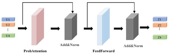
Figure 8.
Schematic Diagram of the TransformerEncoder-Prob Module Architecture.
As shown in Figure 8, Each attention sublayer is followed by residual connection and normalization (Add and Norm). The input feature vector V is transformed into by calculating the attention and normalizing the layer, as shown in Equation (6):
The output is further refined through a feed-forward network (FFN) and another normalization step: (Equation (7)):
Finally, the first time-step representation is extracted as the global feature , which is fed into a fully connected classifier for prediction (Equation (8)):
where denotes the classification results of this channel.
3.3. Inception-Based Feature Extraction Channel (I-Channel)
This section provides a detailed overview of the architectural design of the temporal feature extraction channel (I-Channel) in the SIG-ShapeFormer model, as illustrated in Figure 9. This channel primarily comprises a novel multi-scale Inception module and the previously introduced variant Transformer encoder. The multi-scale Inception module is an innovative convolutional structure that employs parallel multi-branch 1D convolutions to capture both local and global features at different scales. It integrates multi-scale information through feature concatenation. To ensure that critical spatial positional information is preserved during the evolution of cloud patterns, a learnable positional encoding mechanism is introduced.
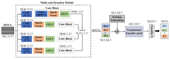
Figure 9.
Schematic diagram of the spatiotemporal transformation feature channel architecture.
The multi-scale fused features are subsequently processed by the enhanced Transformer Encoder-Prob module, which progressively uncovers deeper spatiotemporal dependencies. Ultimately, these features are passed through a base classifier to generate prediction outputs.
3.3.1. Multi-Scale Inception Module Design
The original ShapeFormer model employs one-dimensional convolutions for feature extraction, offering advantages in structural simplicity and computational efficiency. However, its single-scale receptive field limits the effective capture of complex multi-scale spatiotemporal features in satellite cloud imagery. To address this issue, this study proposes an enhanced multi-scale convolutional Inception module. Inspired by the classical Inception architecture, our module integrates convolution kernels ranging from to to simultaneously extract both local and global features. Given that the preprocessed time-series length is 13, we set the maximum convolution kernel size to to avoid performance degradation caused by convolution lengths matching the time-series length. This allows our convolutional model to dynamically adjust based on the preprocessed time-series length, ensuring optimal feature extraction.
Specifically, for time-series data of length 13, the proposed module adopts a four-branch parallel structure and incorporates a hierarchical feature fusion mechanism, significantly enhancing the capability for feature representation. The architecture of the multi-scale convolutional Inception network is illustrated in Figure 10.
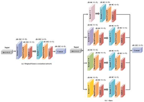
Figure 10.
Comparative schematic diagram of the multi-scale convolutional Inception network architectures: (a) the generic feature extraction module adopted by the Shapeformer model, (b) the temporal feature extraction module implemented in our proposed model.
As illustrated in Figure 10b, the proposed multi-scale Inception module consists of four parallel one-dimensional convolutional branches. Each branch comprises a horizontal convolution (where ) and a basic convolutional block. This convolutional block includes a vertical 1D convolution, followed by a BatchNorm2d layer and a GELU activation function. Specifically, the horizontal 1D convolutions are designed to extract local spatiotemporal features at various scales from the satellite cloud image sequences. Subsequently, the convolutional block compresses the spatial dimension while preserving the temporal dimension and increases the number of channels, thereby enhancing the capacity to capture temporal dependencies. Finally, the outputs of the four branches are concatenated along the channel dimension to achieve multi-scale feature fusion. Given an input tensor , where B is the batch size, C is the number of channels (expanded to 1 before input), V is the feature dimension, and T is the number of time steps, the detailed computational procedure for each branch is described as follows:
Detail Enhancement Branch ( convolution): Utilizes convolutional kernels to expand feature dimensions while preserving critical local details. The process involves a ConvBlock composed of a convolution , BatchNorm, and GELU activation. The Gaussian error linear unit (GELU), defined as , where denotes the standard Gaussian cumulative distribution function, introduces a smooth and probabilistic form of nonlinearity. Unlike the Rectified Linear Unit (ReLU), which zeroes out all negative inputs, GELU adaptively weights each input based on its magnitude. This formulation enhances gradient flow and improves the ability to capture complex feature representations. The resulting feature is calculated as shown in Equation (9).
Short-term Feature Branch ( convolution): Retains the use of convolutional kernels to capture immediate temporal variations, followed by processing through a ConvBlock. The transformation for this branch is represented by Equation (10).
Mid/Long-term Feature Branches ( and convolutions): Employ larger kernels (, ) to model broader spatiotemporal patterns, generating outputs and , respectively.
The outputs of the four branches are concatenated along the channel dimension to form multi-scale fused features . This design not only enhances feature diversity and richness but also improves adaptability to features at different scales, enabling more effective processing of complex spatiotemporal variations in satellite cloud image data.
3.3.2. Positional Encoding and Temporal Modeling
As shown in Figure 9 and the preceding computational process, the fused feature output is denoted as . After transformation, the tensor is reshaped to to match the input format required by subsequent modules. To enhance the modeling of temporal order information, a learnable positional encoding P is added to the transformed features. This design effectively improves the perception of temporal dependencies and strengthens the overall representation learning capability. The enhanced features are then fed into the Transformer Encoder-Prob for deeper spatiotemporal dependency modeling. The Transformer Encoder-Prob progressively extracts and integrates features through multiple layers of ProbAttention and Add and Norm modules, ultimately generating the temporal feature representation , and E is embed size. Let denote the composite operations within the Transformer Encoder-Prob, then can be expressed as = TE(W + P).
Finally, the temporal features are processed by a dedicated base classifier to produce the classification result for the channel, as formalized in Equation (11):
where denotes the classification output of this channel.
3.4. GASF Transformation Channel with Differential Feature Fusion (G-Channel)
To address the limitations of the original ShapeFormer model in spatial feature utilization, this study introduces an innovative spatial feature extraction channel—referred to as the G-channel—in the SIG-ShapeFormer architecture (as illustrated in Figure 11). This channel leverages a Gramian Angular Summation Field (GASF) transformation that incorporates differential information. Specifically, it constructs GASF images from the original sequence, first-order differences, and second-order differences. These three types of GASF images are then integrated into a unified representation through channel fusion techniques [38,39]. Subsequently, a simplified ResNet backbone is employed to extract deep spatial features from the fused GASF image. This design enhances the joint encoding of spatiotemporal information and strengthens the ability to capture complex spatial patterns, thereby overcoming the spatial limitations of the original model. The proposed improvement leads to significant gains in both overall performance and robustness.
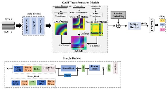
Figure 11.
Schematic Diagram of the Spatial Feature Extraction Channel Architecture.
As shown in Figure 11, given a time series (where to represent observations at different time steps), the data first undergoes preprocessing, including first-order and second-order differencing (calculated via Equation (12)), normalization, and polar coordinate transformation.
To preserve dimensionality after differencing (reducing lengths to and ), mirror padding is applied. All sequences are then normalized to (Equation (13)).
where and denote the mean and standard deviation of the sequence, respectively.
For the normalized time series , we map it to a polar coordinate system and encode temporal phase relationships as 2D spatial correlations via the Gramian Angular Summation Field (GASF). Each element characterizes the joint phase features between time points i and j, with the computational procedure detailed in Equation (14).
The generated GASF feature matrices (all with dimensions ) from the original sequence, first-order difference, and second-order difference undergo average pooling along the feature dimension to produce compressed single-channel matrices: GASForiginal, GASFfirst-order, and GASFsecond-order. These matrices are then stacked along the feature dimension to form a three-channel pseudo-color image representation. This process is formally described by Equation (15):
This multichannel representation effectively captures the dynamic characteristics of time-series variations, thereby significantly improving classification accuracy.
The temporal-spatial information generated through GASF transformation, combined with learnable positional encoding to incorporate spatiotemporal context, is fed into a lightweight ResNet Simple network for spatial feature extraction. This computational process is formalized in Equation (16).
The extracted features are then mapped to the category space through a base classifier layer, yielding the classification result , as formalized in Equation (17).
where is the classification result of this channel.
3.5. EAFM(Ensemble-Attention Feature Mixer) Module
To effectively integrate the preliminary features extracted from the S, I, and G channels and enhance classification accuracy, this study proposes a novel feature fusion framework termed the Ensemble-Attention Feature Mixer (EAFM), as illustrated in Figure 12. The EAFM adopts a two-layer architecture designed to improve the performance of remote sensing image classification. At the first level, heterogeneous base classifiers (S, I, and G channels) extract multimodal features and generate preliminary predictions. The metaclassifier at the second level dynamically integrates these outputs via a self-attention mechanism while preserving the original information flow. Compared with traditional static fusion methods, this framework adaptively adjusts feature weights to effectively capture the varying contributions of each classifier across different meteorological scenarios, significantly improving recognition performance for complex weather systems [40].
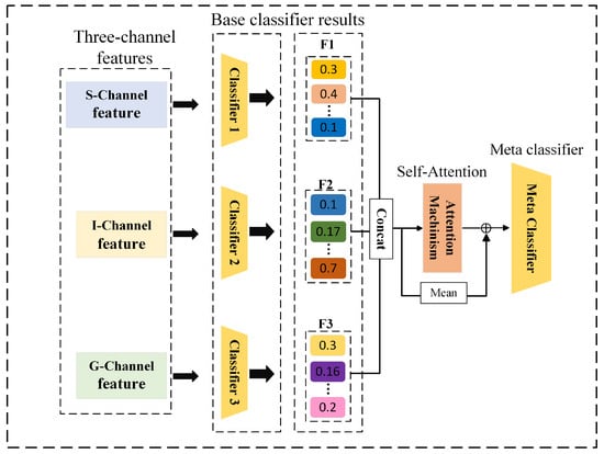
Figure 12.
The overall architecture of the EAFM (Ensemble-Attention Feature Mixer).
As shown in the fourth section of Figure 12, the core of the attention mechanism lies in dynamically fusing multidimensional feature outputs extracted by three base classifiers: shape feature classifier, temporal feature classifier, and GASF feature classifier. This process enhances the accuracy of satellite cloud image recognition through adaptive feature fusion with updated weights adaptively. The specific steps are as follows:
Concatenation of Base Classifier Outputs: Stack the output vectors from the shape feature classifier , temporal feature classifier , and GASF feature classifier to form matrix C (dimensions are batch size B by number of classes d).
Generation of Attention Components: Utilize learnable parameters , , and to generate the Query, Key, and Value required for the attention mechanism.
Computation of Attention Weights: Employing a self-attention mechanism, calculate the importance weights of each feature channel using an average attention weight approach to determine the contribution degree of each base classifier to the final feature representation, as detailed in Equation (18). This step optimizes the feature fusion process, thereby enhancing the capability of the model in recognition.
where is the matrix of attention weights, and represents the attention weights for each of the base classifiers, with d being the output dimension of each base classifier.
Based on the weights of each base classifier, we can dynamically fuse the feature outputs from these classifiers to obtain the final fused feature , as shown in Equation (19). Since the weights of the three base classifiers are involved in the computation of , these weights are automatically adjusted during model training to optimize classification performance.
Finally, the model obtains the final result feature by summing the average of the three base classification outputs with the fused feature , which is dynamically integrated using attention weights. This process is further optimized through residual connections to enhance feature representation. The resulting feature is then passed to the metaclassifier (i.e., the softmax layer) to generate the final prediction output of the model. The calculations for this process are detailed in Equation (20).
This architecture effectively addresses issues of weight allocation bias and information redundancy in multimodal feature fusion through heterogeneous feature decoupling extraction and a dynamic weight adaptive mechanism.
4. Experiments and Results
4.1. Implementation Details
We conducted model evaluation using the publicly available LSCIDMR-S dataset. Due to the significant class imbalance—particularly for Frontal Surface and Westerly Jet, which each contain only about 600 samples—We constructed Dataset 1 for experiments by performing stratified sampling to select a total of 5000 satellite cloud images across all categories (detailed sampling criteria are provided in Section 2). Dataset 1 was divided into training and testing sets in an 8:2 ratio. The class distribution in the experiment is summarized in Table 5.
Table 5.
The categories included in Dataset 1 and the distribution of the corresponding data quantities.
For image-based comparison models, Dataset 1 was used for training and testing. Additionally, these 5000 images were converted into 872 multivariate time-series samples (Dataset 2) for training and testing SIG-ShapeFormer and other sequence-based models, following the conversion method detailed in Section 2. Dataset 2 was also divided into training and testing sets at an 8:2 ratio.
All experiments were conducted using the PyTorch v2.5 framework on an NVIDIA RTX 3070 GPU (32 GB memory). Training parameters were set as follows: batch size of 16, learning rate of 0.001, optimizer RAdam, and cross-entropy loss function. To ensure the comparability of training duration and model convergence, all models were trained for 500 epochs. Evaluation metrics were averaged over five repeated runs to reduce variance, and the best-performing version of each model was retained for confusion matrix analysis. The average cross-entropy loss formula is Equation (21):
where N is the number of samples, C is the number of classes, is the true label, and is the predicted probability. This setup ensures the consistency and validity of the experiments.
4.2. Evaluation Metrics
To evaluate the classification performance of satellite cloud images, this study uses two common metrics: Overall Accuracy (OA) [41] and the confusion matrix. OA indicates the proportion of correctly classified samples among all predictions, providing a clear measure of overall classification performance across all classes. The confusion matrix presents detailed classification results for each class, showing both correct and incorrect predictions. Together, these metrics offer a comprehensive evaluation of classification quality.
Although OA and the confusion matrix are widely adopted in remote sensing classification, they may not fully reflect performance in cases of class imbalance or when both precision and recall are important. Therefore, precision, recall, and F1-score are included as supplementary metrics for a more balanced and detailed assessment [23,34,42]. Precision measures the accuracy of positive predictions by indicating the proportion of predicted positives that are correct. Recall assesses the completeness of detection by measuring the proportion of actual positives that are correctly identified. The F1-score, as the harmonic mean of precision and recall, balances the trade-off between false positives and false negatives, making it particularly useful in imbalanced scenarios or when both error types matter.
These metrics are computed from four key values in the confusion matrix: True Positive (TP), False Positive (FP), False Negative (FN), and True Negative (TN), with the following formulas:
4.3. Comparative Experiment
To validate the effectiveness of the proposed SIG-ShapeFormer, we conducted comprehensive comparisons with a range of state-of-the-art methods based on CNNs, LSTMs, and Transformers. Specifically, the CNN-based methods included ResNet-50 [43] (2016), DenseNet [44] (2017), PCNet [45] (2022), LCNN-BFF [46] (2020), CMUNetx [47] (2023), DTA-Unet [48] (2024), and PFFGCN [49] (2024). The LSTM-based models included TapNet [50] (2020), and MLSTM-FCNS [51] (2019). Transformer-based approaches comprised ViT (2021), ConvTran [52] (2024), TST [53] (2021), SVP-T [54] (2023), and ShapeFormer (2024). The experimental results are presented in Table 6. To comprehensively evaluate model performance on the satellite cloud image classification task, we adopted four standard metrics: precision, recall, F1 score, and overall accuracy(OA).
Table 6.
Performance comparison of different baseline models on the LSCIDMR-S dataset across four evaluation metrics (higher is better). The best result for each metric is indicated in black bold.
As shown in the Table 6, the proposed SIG-ShapeFormer achieved the highest OA of 99.36% on the LSCIDMR-S dataset, surpassing the original ShapeFormer by 2.22%, and was the only model to exceed the 99% accuracy threshold. Moreover, it achieved over 99.40% across precision, recall, and F1-score metrics. Compared to the best-performing CNN-GCN hybrid model, PFFGCN, our model improved OA from 93.50% to 99.36%, with approximately 6% gains in other metrics. These results underscore the advantages of incorporating temporal features, in contrast to traditional CNN-based methods, which focus primarily on spatial structures.
Compared with LSTM-based hybrid models, the performance highlights the importance of modeling time-evolving cloud dynamics. By transforming satellite cloud images into multivariate time series, our model effectively captures temporal patterns through shape trajectory modeling, multi-scale convolutional representations, and GASF-based trend encoding. This allows the model to recognize subtle yet significant transitions within different cloud types, which LSTM models often fail to distinguish when sequences appear similar. Finally, although Transformer-based models demonstrate strong global modeling capacity, their limited ability to capture fine-grained local trends in longer time series affects their classification performance. In contrast, SIG-ShapeFormer combines local and global insights effectively, resulting in consistent improvements across all evaluation criteria. These comprehensive comparisons confirm the superiority and robustness of the proposed SIG-ShapeFormer framework.
As shown in the comparative results presented in Table 6, the proposed SIG-ShapeFormer outperforms other baseline models on the LSCIDMR-S dataset, achieving superior classification performance. In addition to reporting the overall classification accuracy for each model, we further present the confusion matrices of nine representative models in Figure 13. These models cover typical convolutional neural networks (e.g., ResNet, DenseNet, PCNet), hybrid models incorporating LSTM components (e.g., TapNet and MLSTM-FCNS), and Transformer-based architectures (e.g., ShapeFormer and the proposed SIG-ShapeFormer).
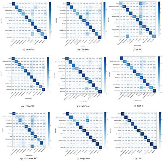
Figure 13.
Confusion Matrices of Optimal Results for Each Model: Subplots (a–i) in the figure show the confusion matrices corresponding to the optimal results of 9 comparative models, respectively.
From Figure 13i, it can be observed that SIG-ShapeFormer achieves consistently strong classification results across 10 out of 11 categories, with the remaining category also exhibiting accuracy close to 90%. This demonstrates the effectiveness of the model in extracting discriminative features within each cloud type and in distinguishing between different categories. The adaptive fusion of multimodal features further enhances the robustness of the model and contributes to its improved accuracy. It is worth noting that the classification performance for the HighiceCloud category remains relatively low across most models, with accuracy often falling below 60%. This may be attributed to high visual similarity with other categories or poor image quality within that class. Furthermore, as shown in Figure 13f,g, LSTM-based hybrid models underperform in several categories, such as HighiceCloud and Westerlyjet, indicating their limited effectiveness in this task. These results suggest that relying solely on temporal modeling is insufficient to capture the key discriminative features in multivariate time series derived from satellite cloud images. Although such data contain temporal components, they do not conform to the properties of conventional time series. Thus, effective classification requires the integration of both spatial structure and temporal evolution information.
Finally, Figure 14 presents a bar chart summarizing the performance of the proposed SIG-ShapeFormer and the baseline models in four evaluation metrics. Precision, F1 score, recall, and overall accuracy. Each model is represented by a group of four bars, distinguished by different colors, from left to right, corresponding to the aforementioned metrics. As illustrated in the figure, the bars associated with SIG-ShapeFormer consistently exhibit the highest height across all four metrics, indicating its superior performance. This further substantiates the effectiveness and robustness of the proposed model in satellite cloud image classification tasks.
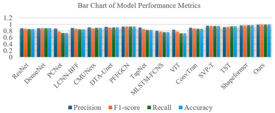
Figure 14.
Performance Comparison of Various Models on Precision, Recall, F1-Score, and Accuracy.
To rigorously evaluate the effectiveness of the proposed feature fusion module, which integrates ensemble learning with an attention mechanism, in comparison to alternative fusion strategies, a comprehensive set of comparative experiments was conducted. The results are summarized in Table 7. The first fusion strategy, referred to as Trichannel + Concat, serves as a baseline method. In this approach, the feature representations extracted from the three individual feature extraction branches are concatenated into a single vector. This concatenated vector is then directly fed into a fully connected layer to produce the final classification output, without involving any base classification components. The second strategy, termed Trichannel + stacking, involves processing each feature channel through a corresponding base classification component. These components generate independent prediction vectors, which are then summed element-wise and passed to a metaclassifier to obtain the final classification result. The third strategy represents the feature fusion method proposed in this study. Building upon the stacking-based approach, an attention mechanism is introduced to perform a weighted combination of the outputs generated by the three base classification components. Specifically, the mechanism dynamically computes adaptive weights based on the discriminative contribution of the output of each component for a given input sample. The resulting weighted sum is used to construct the fused feature representation, which is subsequently fed into the metaclassifier to derive the final classification decision. This strategy effectively captures the varying importance of different feature channels across samples, thereby enabling a more adaptive, discriminative, and robust feature integration process.
Table 7.
Performance comparison of the proposed model under three different feature fusion strategies (all metrics in %). The black bold font denotes the best result for each metric.
As shown in Table 7, the experimental results demonstrate that the proposed fusion framework outperforms conventional feature fusion methods across multiple evaluation metrics. Compared to the baseline approach, which directly concatenates the three feature representations and feeds them into a fully connected layer for classification and achieves an overall accuracy of 0.9828, the stacking-based learning strategy improves the overall accuracy to 0.9885, an improvement of approximately 0.57%. This indicates that by training multiple base classifiers and aggregating their predictions, the stacking strategy effectively enhances the robustness and generalizability of the model. Based on this foundation, the attention-based weighted fusion strategy proposed in this study dynamically assigns adaptive weights to each channel of features based on its relative importance to the current classification task. This mechanism effectively reduces the impact of potentially anomalous or less informative predictions from individual channels while preserving and emphasizing the contributions of more discriminative ones. By enabling adaptive integration of multichannel outputs, the proposed method significantly enhances the overall classification performance, further increasing the overall accuracy to 0.9936.
To provide a more comprehensive evaluation of the proposed SIG-ShapeFormer model, we further analyze the time efficiency and model complexity of all compared methods. Specifically, Table 8 summarizes the average training time per epoch (in minutes) and the total number of trainable parameters (in millions) for each model on the constructed LSCIDMR-S dataset. This comparison facilitates a holistic understanding of the computational cost associated with each model beyond its classification performance.
Table 8.
Training Time per Epoch (min) and Number of Trainable Parameters (M) for Different Models.
As shown in Table 8, although SIG-ShapeFormer introduces additional computational overhead due to the incorporation of multi-scale convolutional blocks and the GASF-based temporal encoding module—resulting in an increase in the number of trainable parameters from 5.2 M in the original ShapeFormer to 7.98 M—it still maintains a reasonable training time and exhibits a moderate model complexity among all compared models. Notably, SIG-ShapeFormer achieves the best performance across all evaluation metrics while preserving favorable computational efficiency, demonstrating a well-balanced trade-off between effectiveness and efficiency.
4.4. Ablation Experiment
To comprehensively investigate the effectiveness of key components in the SIG-ShapeFormer model, we designed and conducted four ablation experiments, evaluating the impact of the multi-scale Inception module, the GASF channel with differential enhancements (FD-order), the standard GASF channel without differential information, and the Ensemble-Attention Feature Mixer (EAFM) module. Specifically, the multi-scale Inception module enhances model performance by capturing multidimensional cloud image sequence features; the GASF channel assesses the contribution of spatial texture encoding, particularly the benefits brought by incorporating first- and second-order differences; and the EAFM framework explores how integrating ensemble learning with attention mechanisms improves feature representation and learning capacity. These investigations aim to quantify each module’s contribution to the overall performance of SIG-ShapeFormer and to provide theoretical foundations for future improvements. The experimental results are summarized in Table 9, which offers quantitative insights into the importance of each module and the overall superiority of the proposed model.
Table 9.
Ablation study results for key components of the proposed model (all metrics in %). The combination of a multi-Inception module, GASF with FD-order difference, and EAFM yields the best performance. The best results in each column are highlighted in bold.
(1) Multi-scale Inception block In the ablation study targeting the multi-scale Inception module, we replaced it with the general feature extraction module used in ShapeFormer while retaining the GASF channel with differential enhancements and the EAFM module. As shown in the first row of Table 9, removing the multi-scale Inception module results in an average decrease of approximately 0.1% in precision (0.9929), recall (0.9930), F1-score (0.9930), and accuracy (0.9928), compared to the complete SIG-ShapeFormer model. This demonstrates that the multi-scale Inception module effectively improves the ability of the model to capture multi-granularity features.
(2) GASF channel after integrating differential information In the ablation study targeting the GASF transformation channel with integrated differential information, we constructed a dual-channel model that retains only the Shapelet and multi-scale Inception modules. According to the second row of Table 9, removing the GASF channel results in precision, recall, F1-score, and accuracy dropping to 0.9870, 0.9860, 0.9860, and 0.9857, respectively, with an overall performance decrease of approximately 0.8%. This indicates that the GASF channel plays a crucial role in integrating differential information and extracting spatial features.
(3) FD-order In the ablation study of the GASF transformation process that integrates first- and second-order differential information, we directly applied the GASF transformation to the satellite cloud image sequences without incorporating differential information. According to the third row of Table 9, removing the differential information causes the precision, recall, F1-score, and accuracy to drop to 0.9930, 0.9828, 0.9928, and 0.9929, respectively, reflecting an average performance decrease of approximately 0.1%. This shows that integrating differential information during GASF transformation improves the ability to extract spatial texture and transformation trend characteristics. To better demonstrate the ability of the GASF transformation to capture spatial characteristics between different classes, Figure 15 presents the GASF matrices generated from a time series of satellite cloud images representing ten categories in the dataset. Specifically, for each class, the time series corresponding to the first feature was selected. Each GASF image is accompanied by a vertical color bar on the right, indicating the normalized value range from (blue) to +1 (yellow), which corresponds to the angular summation values defined in Equation (14).

Figure 15.
GASF-transformed images of ten satellite cloud sequences: (a) Extratropical Cyclone, (b) Low-Water Cloud, (c) Snow, (d) High-Ice Cloud, (e) Tropical Cyclone, (f) Frontal Surface, (g) Desert, (h) Vegetation, (i) Ocean, (j) Westerly Jet.
Figure 15 demonstrates significant differences and unique patterns in GASF-transformed images across various cloud types. For instance, low-water cloud and high-ice cloud exhibit distinct cross-shaped structures in their first- and second-order difference images, likely reflecting internal homogeneity and stability. In contrast, the Westerly Jet displays different characteristics: its original sequence shows clear diagonal patterns, indicating strong positive correlations and temporal stability, consistent with its persistent and unidirectional nature in atmospheric circulation. The first-order difference images reveal cross structures and banded features, demonstrating consistent variation trends over specific time periods, while the second-order difference images highlight localized concentration in variation rates, with directional and periodic dynamic patterns despite scattered high-value regions. This contrast not only reveals fundamental distinctions between cloud types but also provides visual evidence for identifying large-scale circulation versus local cloud systems.
(4) EAFM block In the ablation study of the feature fusion module (EAFM) of the model, we removed the EAFM component and directly used a fully connected layer to classify the concatenated features. As shown in the fifth row of Table 9, this modification results in a performance drop, with the overall accuracy decreasing to 0.9857—approximately 0.86% lower than the complete SIG-ShapeFormer model, and even below the accuracy of the dual-channel model used in Ablation Experiment 2 (0.9928). These results demonstrate that the absence of dynamic weight allocation from the attention mechanism and the multimodal fusion capability offered by ensemble learning severely limits the ability to integrate information effectively and achieve optimal performance. To better visualize the contribution of each channel feature to the final classification outcome, we saved the normalized attention weights of each base classifier at every epoch during the training process. The model was trained for a total of 500 epochs, resulting in weight change curves for each base classifier, as shown in Figure 16.
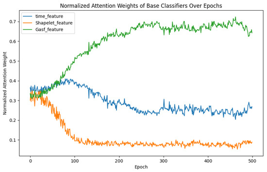
Figure 16.
Weight Change Curves of Features from Each Channel: The time_feature, Shapelet_feature, and GASF_feature curves represent the classification result features extracted from the Inception (I) channel, Shapelet (S) channel, and GASF (G) channel, respectively.
Based on the analysis of the weight change curves shown in Figure 16, the importance weights of the three feature extraction channels during model training exhibit the following dynamic changes:
- Shapelet Feature Channel: The weight of this channel gradually decreases, indicating its significant value in identifying critical spatiotemporal patterns (such as unique subsequences in weather systems) during the early stages of training. However, its relative importance diminishes as the model learns more robust multi-scale features through other channels, such as GASF.
- Multi-Scale Inception Channel: From epoch 100 onwards, the weight of this channel stabilizes and converges to approximately 0.3. This highlights the consistent support provided by its multi-scale convolutional kernels for capturing fine and coarse spatiotemporal features.
- GASF Transformation Channel: As training progresses, the weight of this channel increases and stabilizes at around 0.6, demonstrating its capability to integrate first/second-order differential information and spatial structural features, which is crucial for enhancing classification accuracy.
4.5. Generalization Experiment
To evaluate the generalization capability of the proposed model, we conducted systematic experiments on two categories of datasets with distinct characteristics. First, to assess the effectiveness of the model in remote sensing image classification tasks, we selected the widely used benchmark dataset UCM for generalization testing, with overall accuracy (OA) adopted as the primary evaluation metric.
Given that the UCM dataset lacks an explicit temporal dimension and does not exhibit temporal continuity, it is not suitable for fully exploiting the strengths of the multivariate time-series modeling modules designed in this study. Therefore, in this experiment, we compared the proposed model and ShapeFormer—both of which were adapted using the pseudo-time-series transformation method described in Section 2—with CNN-based baseline models capable of directly processing satellite cloud imagery. In the experiments, the UCM dataset was divided into training and testing subsets with a ratio of 8:2. All models were trained for 200 epochs using a unified learning rate of 0.001 and a batch size of 16. The corresponding results are presented in Table 10.
Table 10.
Performance comparison of different models on the UCM dataset across four evaluation metrics (all metrics in %). The best results in each column are highlighted in bold.
In addition, considering that the proposed model is designed to process multivariate time series as input, we further selected seven representative datasets from the UEA Multivariate Time-Series Archive [55] to conduct a comprehensive evaluation of generalization performance. Four evaluation metrics, including overall accuracy, were employed. Since these datasets are in pure multivariate time-series format, traditional convolution-based models designed for static image processing are not directly applicable. As such, these models were excluded from the comparison. Instead, we conducted fair comparisons with other baseline models capable of temporal modeling. The results of these experiments are reported in Table 11. To ensure the comparability and reliability of the results, consistent data partitioning strategies and identical hyperparameter settings were applied across all tasks.
Table 11.
Classification accuracy (%) of different methods on the UEA benchmark datasets (Overall Accuracy; higher values are better), with the best results highlighted in bold.
As shown in Table 11, which presents the generalization results for multivariate time-series classification, the proposed SIG-ShapeFormer outperformed six competing models on four of the seven benchmark datasets—specifically, Heartbeat, StandWalkJump, Libras, and RacketSports—in terms of classification accuracy. These results demonstrate that SIG-ShapeFormer achieves strong generalization performance in multivariate time-series classification and confirm its effectiveness across a variety of complex temporal data domains.
As shown in Table 10, the proposed SIG-ShapeFormer achieved the highest classification accuracy among ten competing models, with an overall accuracy (OA) of 0.9350. The UCM dataset consists of static images that lack continuous temporal information, which is in contrast to satellite cloud image data that inherently exhibit temporal dynamics. Due to this limitation, the performance of the model on the UCM dataset is constrained, with the OA reaching approximately 93%. Several other models, including DenseNet, CMUNetx, DTA-Unet, and ShapeFormer, also demonstrated competitive accuracy levels, achieving results close to 92%.
The experimental results demonstrate that the SIG-ShapeFormer model exhibits a distinct dual-characteristic performance pattern. On the one hand, across eight benchmark datasets (including remote sensing imagery and UEA multivariate time series), the model consistently outperforms most competing methods, thereby validating the strong cross-domain generalization capability of its multi-scale feature fusion mechanism. However, the performance of the model shows a clear positive correlation with the temporal continuity of the input data. When applied to data with well-defined temporal evolution patterns (such as meteorological satellite cloud image sequences), SIG-ShapeFormer effectively leverages its spatiotemporal feature fusion architecture to achieve superior classification accuracy. This performance pattern indicates that although the model demonstrates strong general-purpose applicability, its core innovations (such as the differencing-enhanced GASF transformation and the multi-scale Inception module) offer unique advantages when dealing with data exhibiting strong temporal dependencies. Future research will focus on further optimizing the model architecture to enhance its performance on datasets with weak temporal correlations while maintaining its sensitivity to temporal features.
5. Discussion and Conclusions
This study proposes a high-accuracy satellite cloud image classification model named SIG-ShapeFormer, built upon the ShapeFormer architecture. The model introduces a three-stream feature extraction framework to effectively model complex spatiotemporal information. First, a customized Inception-like module is employed to enhance feature extraction capability, enabling simultaneous capture of both local details and global patterns across multiple scales. This design significantly improves the model’s adaptability to the intricate spatiotemporal variations inherent in satellite cloud imagery. Second, a novel GASF transformation module is developed by integrating first- and second-order differencing to extract spatial evolution features. This component addresses the limitations of the original model in spatial representation and better captures the dynamic progression of cloud image sequences. Finally, an Ensemble-Attention Feature Mixer (EAFM) is proposed to dynamically weigh and fuse multichannel features through an attention mechanism, overcoming the limitations of traditional static fusion strategies under different modalities. Experimental results demonstrate that SIG-ShapeFormer achieves outstanding classification performance and generalization ability across the LSCIDMR-S dataset, several multivariate time-series datasets, and the UCM remote sensing dataset, thereby validating the effectiveness and applicability of the proposed approach.
Despite its strong performance, SIG-ShapeFormer presents certain limitations. First, the model exhibits a strong dependence on the temporal continuity of the input data; its advantages are best realized when dealing with data characterized by clear time-series evolution. The current experiments are primarily conducted on the temporally structured LSCIDMR-S dataset, and further validation on diverse types of time-series remote sensing data is needed. Second, the transformation of cloud image sequences into multivariate time series may lead to the loss of intrinsic spatial structure. Although the GASF transformation captures the trend of cloud development, the spatial modeling within individual image frames remains limited. Furthermore, converting cloud imagery into multivariate sequences causes a rapid increase in feature dimensionality with sequence length, leading to considerable computational cost and extended training time.
To address these challenges, future research will focus on several key directions. On the one hand, we aim to validate the model on a broader range of cloud image datasets with temporal variations to further assess its generalizability and robustness, including its adaptability to remote sensing images with varying spatial resolutions. On the other hand, we plan to optimize the model architecture to reduce its dependence on temporally continuous data, thereby enabling it to handle non-sequential or weakly sequential image data. In addition, we will explore 3D spatiotemporal encoding schemes or hybrid architectures to facilitate end-to-end classification of remote sensing cloud images while preserving more of the original spatial information. In addition, strategies such as sparse attention mechanisms, feature dimensionality reduction, and lightweight network design will be investigated to mitigate the problem of dimensional explosion caused by long sequences and to improve computational efficiency. Finally, the remote sensing satellite cloud image datasets used in this study consist exclusively of high-resolution, large-scale imagery. Future work will involve conducting additional experiments on cloud images of varying resolutions to further evaluate the applicability and generalization capability of the model in multi-scale remote sensing image classification tasks.
The outcomes of this research not only provide a novel technical framework for recognizing complex meteorological systems but also offer a transferable methodology for intelligent classification tasks in remote sensing. Specifically, the model can support automatic labeling of satellite cloud imagery, significantly improving the efficiency of manual annotation. It is also capable of detecting extreme weather events with temporal continuity—such as thunderstorms and strong winds—thus contributing to more effective disaster warning systems. Furthermore, the proposed multimodal fusion framework exhibits promising transferability and can be extended to interdisciplinary domains such as ecological monitoring and ocean remote sensing. It offers methodological insights for the fusion analysis of multi-source heterogeneous data in Earth system science, presenting broad application prospects and research value.
Author Contributions
Conceptualization, X.L. and Z.L. (Zhenyu Lu); methodology and software, X.L.; validation, B.L. and X.L.; formal analysis, Z.L. (Zhenyu Lu); investigation, X.L.; resources, Z.L. (Zhuang Li) and Y.M.; data curation and visualization, B.L. and Z.C.; writing—original draft preparation, X.L.; writing—review and editing, X.L.; supervision, Z.L. (Zhenyu Lu); project administration, X.L. All authors have read and agreed to the published version of the manuscript.
Funding
This research was supported by the Joint Fund of Zhejiang Provincial Natural Science Foundation Project (NO.LZJMD25D050002), the National Natural Science Foundation of China (Key Program) (NO.U20B2061), the National Key Research and Development Program of China (NO.2022ZD012000).
Data Availability Statement
The data are available from the corresponding author upon request.
Acknowledgments
The authors wish to express their gratitude to Remote Sensing, as well as to the anonymous reviewers who helped to improve this paper through their thorough review.
Conflicts of Interest
The authors declare no conflicts of interest.
References
- Zhuang, Z.; Wang, M.; Wang, K.; Li, S.; Wu, J. Research progress of deep learning-based cloud classification. Nanjing Xinxi Gongcheng Daxue Xuebao 2022, 14, 566–578. [Google Scholar]
- Yashuai, F.; Wenhao, Z.; Yongtao, J.; Qiyue, L.; Lili, Z.; Fangfei, B.; Yu, M. Research progress of cloud classification based on optical satellite remote sensing. J. Atmos. Environ. Opt. 2025, 20, 1. [Google Scholar]
- Cheng, Z.; Wang, H.; Bai, J. A Review of Ground-Based Retrieval of Cloud Microphysical Parameters. Meteorol. Sci. Technol. 2007, 35, 9–14. [Google Scholar]
- Ding, L.; Xia, M.; Lin, H.; Hu, K. Multi-level attention interactive network for cloud and snow detection segmentation. Remote Sens. 2023, 16, 112. [Google Scholar] [CrossRef]
- Wang, Y.; Shu, Z.; Feng, Y.; Liu, R.; Cao, Q.; Li, D.; Wang, L. Enhancing Cross-Domain Remote Sensing Scene Classification by Multi-Source Subdomain Distribution Alignment Network. Remote Sens. 2025, 17, 1302. [Google Scholar] [CrossRef]
- Yang, C.; Yuan, Z.; Gu, S. Cloud classification of GMS-5 satellite imagery by the use of multispectral threshold technique. J. Nanjing Inst. Meteorol 2002, 25, 747–754. [Google Scholar]
- Zhou, X.; Yang, X.; Yao, X. The study of cloud classification and detection in remote sensing image. J. Graph. 2014, 35, 768. [Google Scholar]
- Li, J.; Menzel, W.P.; Yang, Z.; Frey, R.A.; Ackerman, S.A. High-spatial-resolution surface and cloud-type classification from MODIS multispectral band measurements. J. Appl. Meteorol. 2003, 42, 204–226. [Google Scholar] [CrossRef]
- Wu, Y.; Zhang, R.; Jiang, G.; Sun, Z.; Niu, S. A fuzzy clustering method for multi-spectral satellite images. J. Trop. Meteorol. 2004, 20, 689–696. [Google Scholar]
- Li, Q.; Zhang, Z.; Lu, W.; Yang, J.; Ma, Y.; Yao, W. From pixels to patches: A cloud classification method based on a bag of micro-structures. Atmos. Meas. Tech. 2016, 9, 753–764. [Google Scholar] [CrossRef]
- Yu, Z.; Ma, S.; Han, D.; Li, G.; Gao, D.; Yan, W. A cloud classification method based on random forest for FY-4A. Int. J. Remote Sens. 2021, 42, 3353–3379. [Google Scholar] [CrossRef]
- Tan, Z.; Liu, C.; Ma, S.; Wang, X.; Shang, J.; Wang, J.; Ai, W.; Yan, W. Detecting multilayer clouds from the geostationary advanced Himawari imager using machine learning techniques. IEEE Trans. Geosci. Remote Sens. 2021, 60, 4103112. [Google Scholar] [CrossRef]
- Zhang, C.; Zhuge, X.; Yu, F. Development of a high spatiotemporal resolution cloud-type classification approach using Himawari-8 and CloudSat. Int. J. Remote Sens. 2019, 40, 6464–6481. [Google Scholar] [CrossRef]
- Shan, W.; Chu-yi, X.; Chun-xiang, S.; Ying, Z. Study on Cloud Classification Method of Satellite Cloud Images Based on CNN-LSTM. Comput. Sci. 2022, 49, 675–679. [Google Scholar]
- Zhang, J.; Liu, P.; Zhang, F.; Song, Q. CloudNet: Ground-based cloud classification with deep convolutional neural network. Geophys. Res. Lett. 2018, 45, 8665–8672. [Google Scholar] [CrossRef]
- Liu, S.; Li, M.; Zhang, Z.; Cao, X.; Durrani, T.S. Ground-based cloud classification using task-based graph convolutional network. Geophys. Res. Lett. 2020, 47, e2020GL087338. [Google Scholar] [CrossRef]
- Afzali Gorooh, V.; Kalia, S.; Nguyen, P.; Hsu, K.l.; Sorooshian, S.; Ganguly, S.; Nemani, R.R. Deep neural network cloud-type classification (DeepCTC) model and its application in evaluating PERSIANN-CCS. Remote Sens. 2020, 12, 316. [Google Scholar] [CrossRef]
- Chen, L.; Xu, D.; Yang, L.; Ng, C.T.; Fu, J.; He, Y.; He, Y. Classification and identification of extreme wind events by CNNs based on Shapelets and improved GASF-GADF. J. Wind. Eng. Ind. Aerodyn. 2024, 253, 105852. [Google Scholar] [CrossRef]
- Li, K.; Yan, H.; Gu, J.; Su, L.; Su, W.; Xue, Z. A Multi-Source Transfer Learning Method for Rolling Bearing Fault Diagnosis Based on Shapelet Time Series. Chin. J. Mech. Eng. 2022, 33, 2990–2996. [Google Scholar]
- Arul, M.; Kareem, A. Applications of shapelet transform to time series classification of earthquake, wind and wave data. Eng. Struct. 2021, 228, 111564. [Google Scholar] [CrossRef]
- Roscher, R.; Waske, B. Shapelet-based sparse representation for landcover classification of hyperspectral images. IEEE Trans. Geosci. Remote Sens. 2015, 54, 1623–1634. [Google Scholar] [CrossRef]
- He, W.; Cheng, M.; Liu, Q.; Li, Z. Shapewordnet: An interpretable shapelet neural network for physiological signal classification. In Proceedings of the International Conference on Database Systems for Advanced Applications, Tianjin, China, 17–20 April 2023; pp. 353–369. [Google Scholar]
- Duan, Y.; Song, C.; Zhang, Y.; Cheng, P.; Mei, S. STMSF: Swin Transformer with Multi-Scale Fusion for Remote Sensing Scene Classification. Remote Sens. 2025, 17, 668. [Google Scholar] [CrossRef]
- Zheng, F.; Lin, S.; Zhou, W.; Huang, H. A lightweight dual-branch swin transformer for remote sensing scene classification. Remote Sens. 2023, 15, 2865. [Google Scholar] [CrossRef]
- Dang, G.; Mao, Z.; Zhang, T.; Liu, T.; Wang, T.; Li, L.; Gao, Y.; Tian, R.; Wang, K.; Han, L. Joint superpixel and Transformer for high resolution remote sensing image classification. Sci. Rep. 2024, 14, 5054. [Google Scholar] [CrossRef]
- Chen, K.; Liu, C.; Chen, H.; Zhang, H.; Li, W.; Zou, Z.; Shi, Z. RSPrompter: Learning to prompt for remote sensing instance segmentation based on visual foundation model. IEEE Trans. Geosci. Remote Sens. 2024, 62, 1–17. [Google Scholar] [CrossRef]
- Chen, K.; Liu, C.; Chen, B.; Li, W.; Zou, Z.; Shi, Z. Dynamicvis: An efficient and general visual foundation model for remote sensing image understanding. arXiv 2025, arXiv:2503.16426. [Google Scholar]
- Chen, K.; Chen, B.; Liu, C.; Li, W.; Zou, Z.; Shi, Z. Rsmamba: Remote sensing image classification with state space model. IEEE Geosci. Remote Sens. Lett. 2024, 21, 8002605. [Google Scholar] [CrossRef]
- Bao, M.; Lyu, S.; Xu, Z.; Zhou, H.; Ren, J.; Xiang, S.; Li, X.; Cheng, G. Vision Mamba in Remote Sensing: A Comprehensive Survey of Techniques, Applications and Outlook. arXiv 2025, arXiv:2505.00630. [Google Scholar]
- Paranjape, J.N.; De Melo, C.; Patel, V.M. A mamba-based siamese network for remote sensing change detection. In Proceedings of the 2025 IEEE/CVF Winter Conference on Applications of Computer Vision (WACV), Tucson, AZ, USA, 28 February–4 March 2025; pp. 1186–1196. [Google Scholar]
- Bai, C.; Zhao, D.; Zhang, M.; Zhang, J. Multimodal information fusion for weather systems and clouds identification from satellite images. IEEE J. Sel. Top. Appl. Earth Obs. Remote Sens. 2022, 15, 7333–7345. [Google Scholar] [CrossRef]
- An, S.; Zhang, L.; Li, X.; Zhang, G.; Li, P.; Zhao, K.; Ma, H.; Lian, Z. Global–Local Feature Fusion of Swin Kansformer Novel Network for Complex Scene Classification in Remote Sensing Images. Remote Sens. 2025, 17, 1137. [Google Scholar] [CrossRef]
- Zhao, H.; Lu, Z.; Sun, S.; Wang, P.; Jia, T.; Xie, Y.; Xu, F. Classification of Large Scale Hyperspectral Remote Sensing Images Based on LS3EU-Net++. Remote Sens. 2025, 17, 872. [Google Scholar] [CrossRef]
- Bai, C.; Zhang, M.; Zhang, J.; Zheng, J.; Chen, S. LSCIDMR: Large-scale satellite cloud image database for meteorological research. IEEE Trans. Cybern. 2021, 52, 12538–12550. [Google Scholar] [CrossRef] [PubMed]
- Yuan, L.; Chen, Y.; Wang, T.; Yu, W.; Shi, Y.; Jiang, Z.H.; Tay, F.E.; Feng, J.; Yan, S. Tokens-to-token vit: Training vision transformers from scratch on imagenet. In Proceedings of the IEEE/CVF International Conference on Computer Vision, Montreal, BC, Canada, 11–17 October 2021; pp. 558–567. [Google Scholar]
- Le, X.M.; Luo, L.; Aickelin, U.; Tran, M.T. Shapeformer: Shapelet transformer for multivariate time series classification. In Proceedings of the 30th ACM SIGKDD Conference on Knowledge Discovery and Data Mining, Barcelona, Spain, 25–29 August 2024; pp. 1484–1494. [Google Scholar]
- Zhou, H.; Zhang, S.; Peng, J.; Zhang, S.; Li, J.; Xiong, H.; Zhang, W. Informer: Beyond efficient transformer for long sequence time-series forecasting. In Proceedings of the AAAI Conference on Artificial Intelligence, Online, 2–9 February 2021; Volume 35, pp. 11106–11115. [Google Scholar]
- Cui, Y.; Wang, R.; Si, Y.; Zhang, S.; Wang, Y.; Lin, A. T-type inverter fault diagnosis based on GASF and improved AlexNet. Energy Rep. 2023, 9, 2718–2731. [Google Scholar] [CrossRef]
- Su, B.; Liu, D.; Chen, Q.; Han, D.; Wu, J. A Method for Identifying Wheat Stripe Rust Resistance Levels Based on Time Series Vegetation Index. Trans. Chin. Soc. Agric. Eng. 2024, 40, 155–165. [Google Scholar]
- Yu, D.; Zhang, B.; Zhao, C.; Guo, H.; Lu, J. Remote Sensing Image Scene Classification Using Convolutional Neural Networks and Ensemble Learning. J. Remote Sens. 2021, 24, 717–727. [Google Scholar]
- Juba, B.; Le, H.S. Precision-recall versus accuracy and the role of large data sets. In Proceedings of the AAAI Conference on Artificial Intelligence, Hilton Hawaiian Village, HI, USA, 27 January–1 February 2019; Volume 33, pp. 4039–4048. [Google Scholar]
- Sekrecka, A.; Karwowska, K. Classical vs. Machine Learning-Based Inpainting for Enhanced Classification of Remote Sensing Image. Remote Sens. 2025, 17, 1305. [Google Scholar] [CrossRef]
- He, K.; Zhang, X.; Ren, S.; Sun, J. Deep residual learning for image recognition. In Proceedings of the IEEE Conference on Computer Vision and Pattern Recognition, Las Vegas, NV, USA, 27–30 June 2016; pp. 770–778. [Google Scholar]
- Huang, G.; Liu, Z.; Van Der Maaten, L.; Weinberger, K.Q. Densely connected convolutional networks. In Proceedings of the IEEE Conference on Computer Vision and Pattern Recognition, Honolulu, HI, USA, 21–26 July 2017; pp. 4700–4708. [Google Scholar]
- Chen, X.; Zheng, X.; Zhang, Y.; Lu, X. Remote Sensing Scene Classification by Local–Global Mutual Learning. IEEE Geosci. Remote Sens. Lett. 2022, 19, 6506405. [Google Scholar] [CrossRef]
- Shi, C.; Wang, T.; Wang, L. Branch feature fusion convolution network for remote sensing scene classification. IEEE J. Sel. Top. Appl. Earth Obs. Remote Sens. 2020, 13, 5194–5210. [Google Scholar] [CrossRef]
- Tang, F.; Ding, J.; Wang, L.; Ning, C.; Zhou, S.K. CMUNeXt: An Efficient Medical Image Segmentation Network based on Large Kernel and Skip Fusion. arXiv 2023, arXiv:2308.01239. [Google Scholar]
- Li, Y.; Yan, B.; Hou, J.; Bai, B.; Huang, X.; Xu, C.; Fang, L. UNet based on dynamic convolution decomposition and triplet attention. Sci. Rep. 2024, 14, 271. [Google Scholar] [CrossRef]
- Zhang, C.; Wang, B. Progressive Feature Fusion Framework Based on Graph Convolutional Network for Remote Sensing Scene Classification. IEEE J. Sel. Top. Appl. Earth Obs. Remote Sens. 2024, 17, 3270–3284. [Google Scholar] [CrossRef]
- Zhang, X.; Gao, Y.; Lin, J.; Lu, C.T. Tapnet: Multivariate time series classification with attentional prototypical network. In Proceedings of the AAAI Conference on Artificial Intelligence, New York, NY, YSA, 7–12 February 2020; Volume 34, pp. 6845–6852. [Google Scholar]
- Karim, F.; Majumdar, S.; Darabi, H.; Harford, S. Multivariate LSTM-FCNs for time series classification. Neural Netw. 2019, 116, 237–245. [Google Scholar] [CrossRef] [PubMed]
- Foumani, N.M.; Tan, C.W.; Webb, G.I.; Salehi, M. Improving position encoding of transformers for multivariate time series classification. Data Min. Knowl. Discov. 2024, 38, 22–48. [Google Scholar] [CrossRef]
- Zerveas, G.; Jayaraman, S.; Patel, D.; Bhamidipaty, A.; Eickhoff, C. A transformer-based framework for multivariate time series representation learning. In Proceedings of the 27th ACM SIGKDD Conference on Knowledge Discovery & Data Mining, Online, 14–18 August 2021; pp. 2114–2124. [Google Scholar]
- Zuo, R.; Li, G.; Choi, B.; Bhowmick, S.S.; Mah, D.N.y.; Wong, G.L. SVP-T: A shape-level variable-position transformer for multivariate time series classification. In Proceedings of the AAAI Conference on Artificial Intelligence, Washington, DC, USA, 7–14 February 2023; Volume 37, pp. 11497–11505. [Google Scholar]
- Bagnall, A.; Dau, H.A.; Lines, J.; Flynn, M.; Large, J.; Bostrom, A.; Southam, P.; Keogh, E. The UEA multivariate time series classification archive. arXiv 2018, arXiv:1811.00075. [Google Scholar]
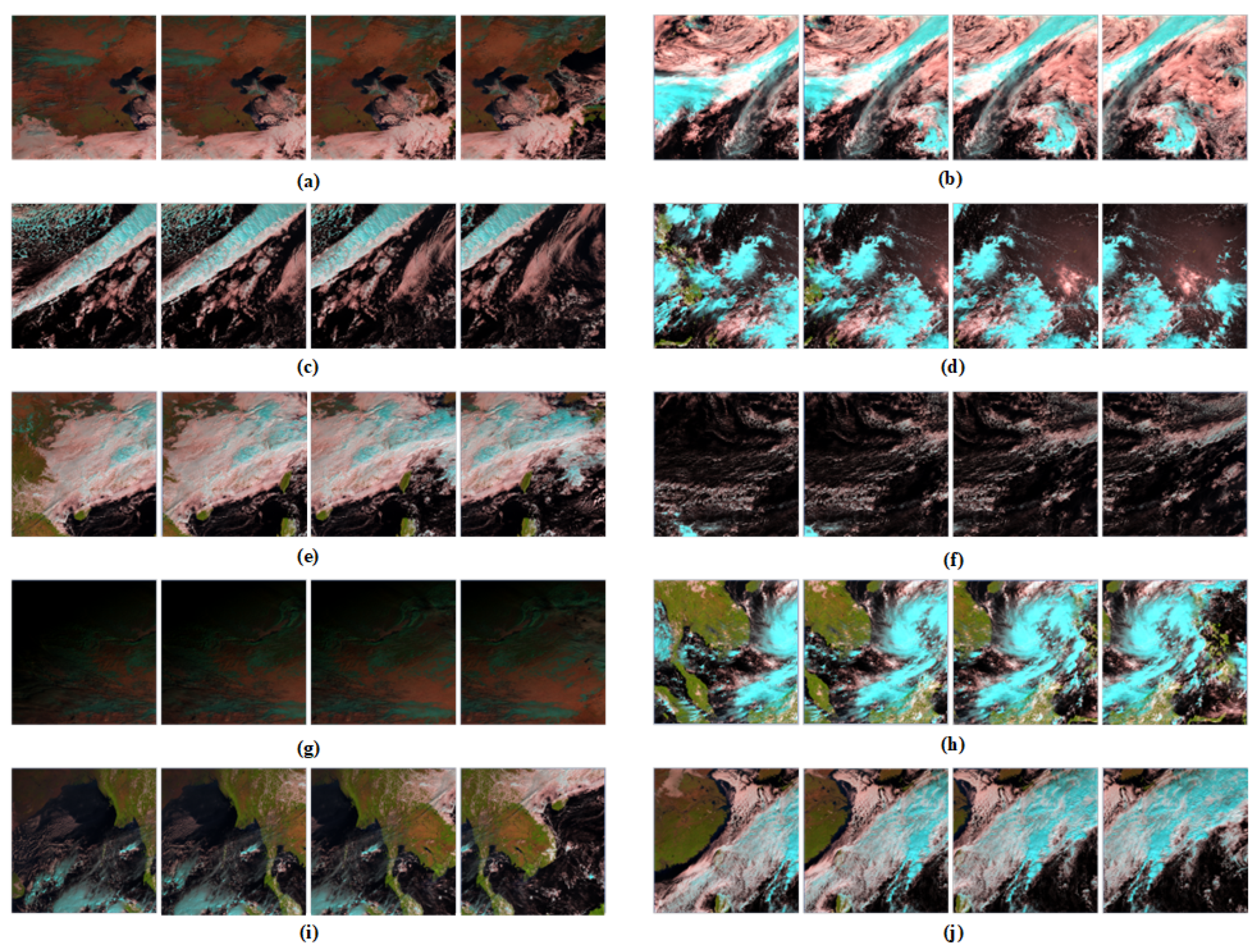

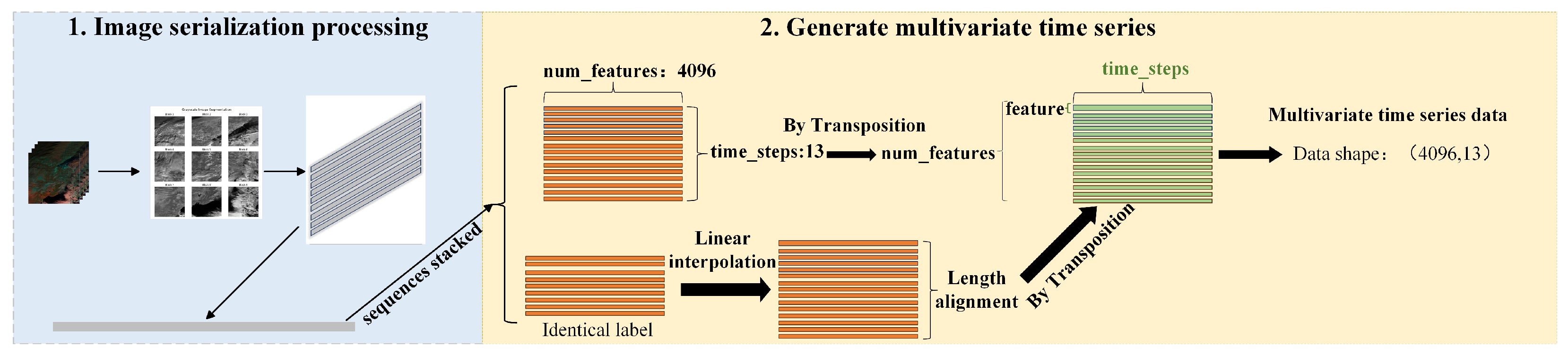

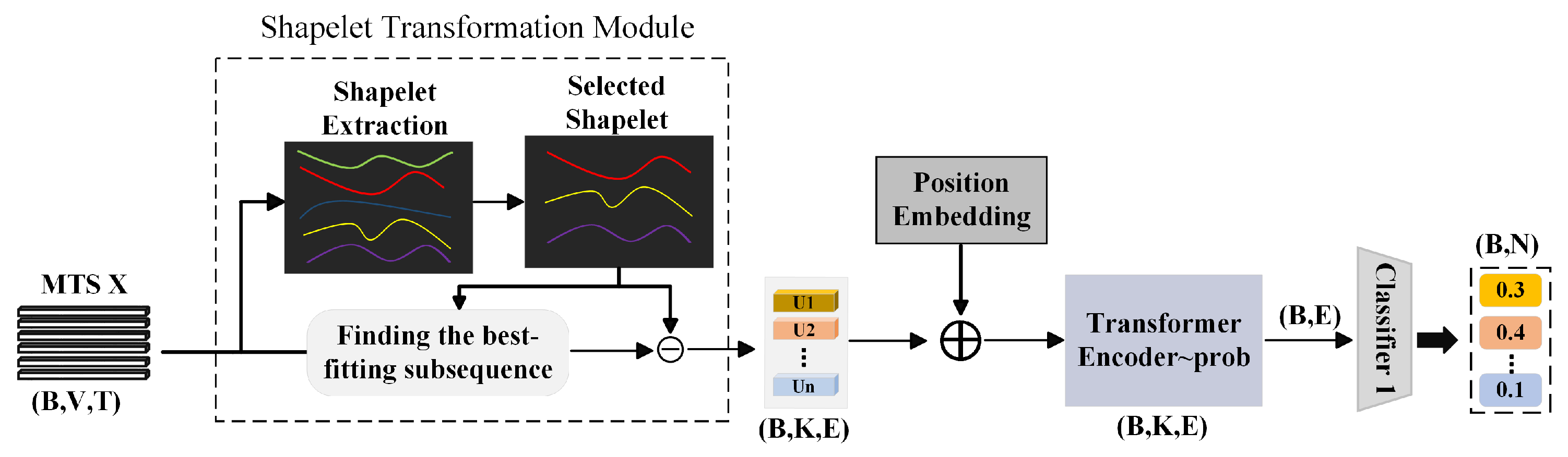
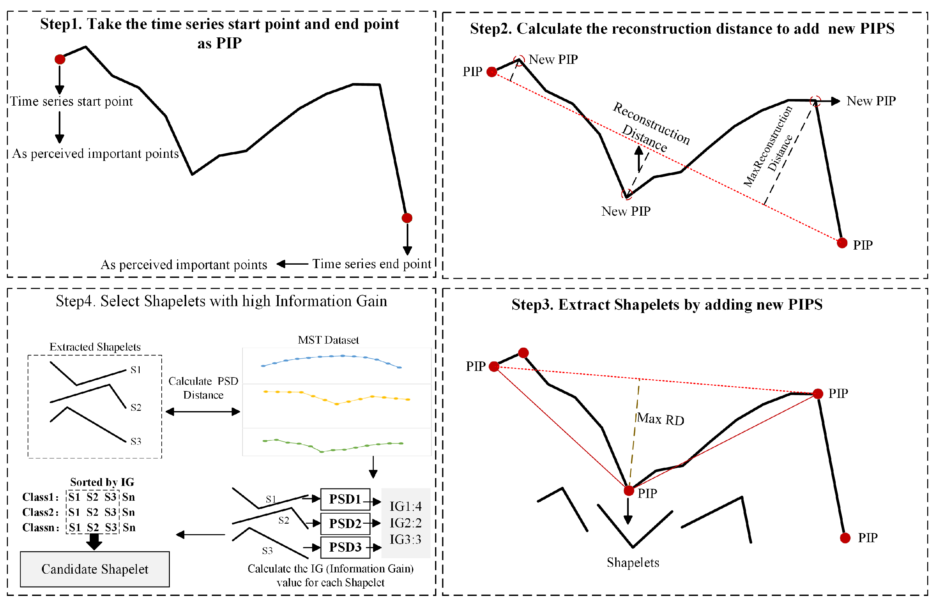
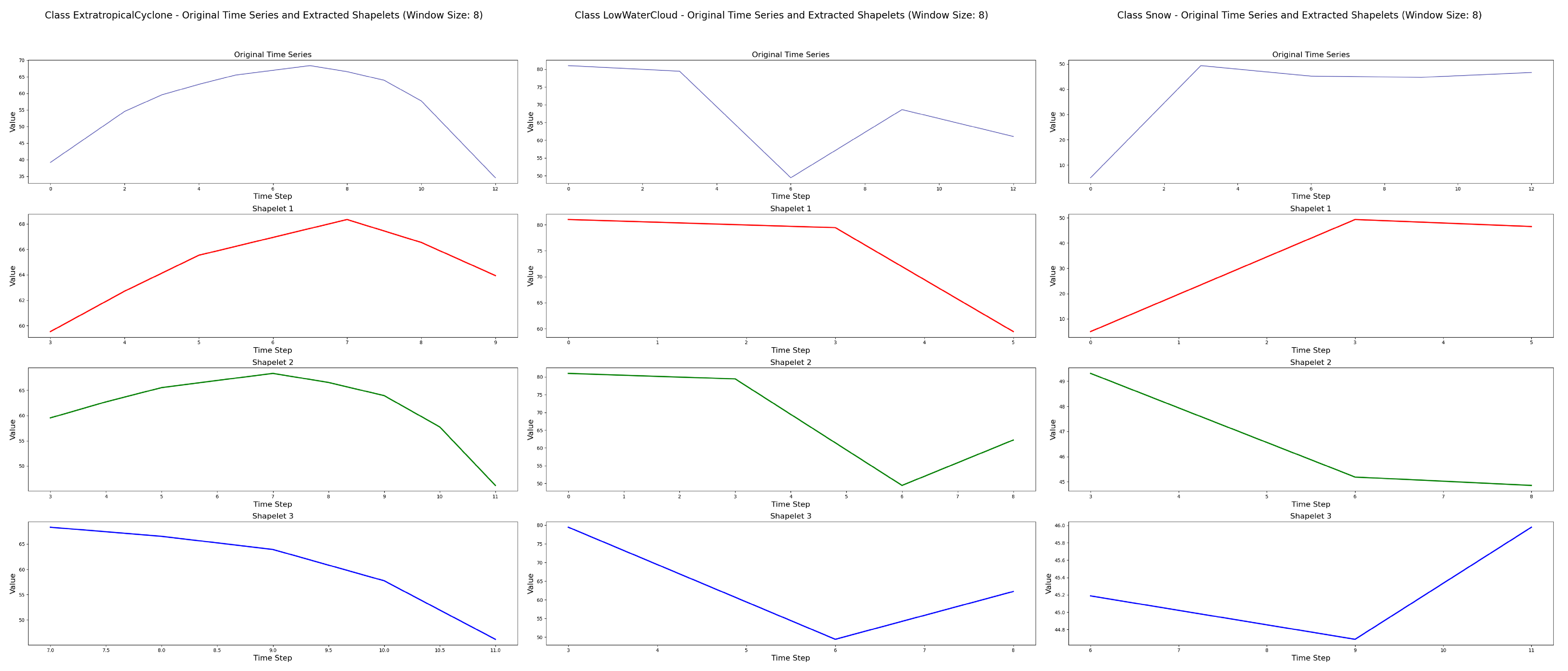
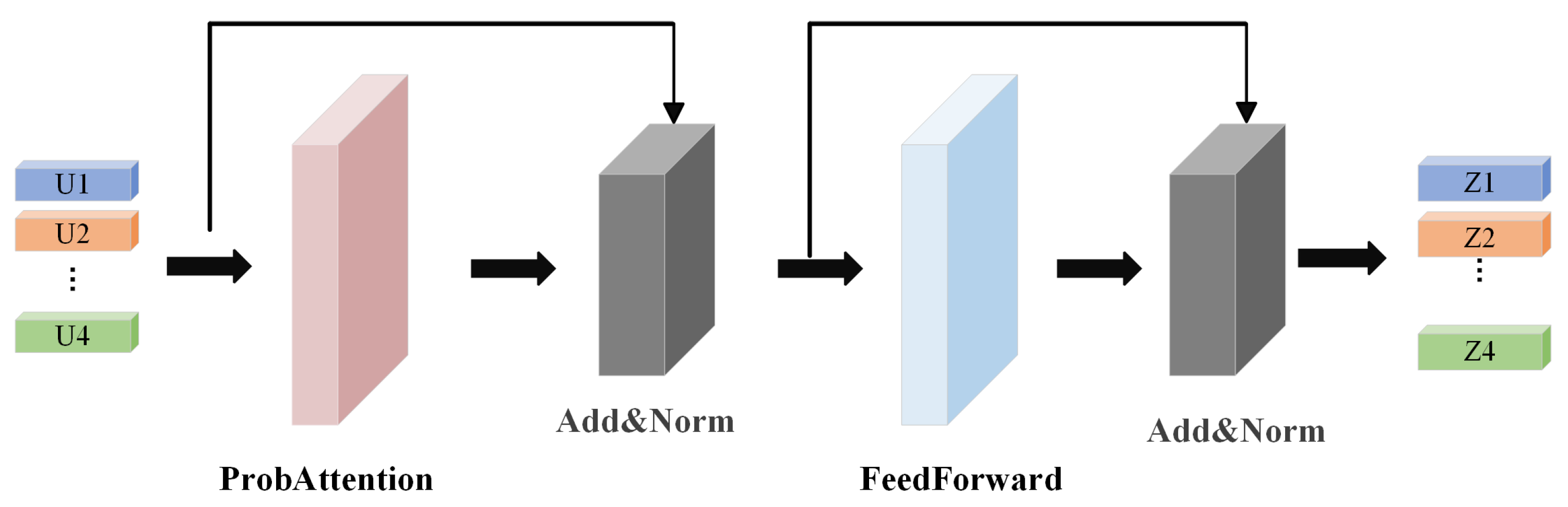

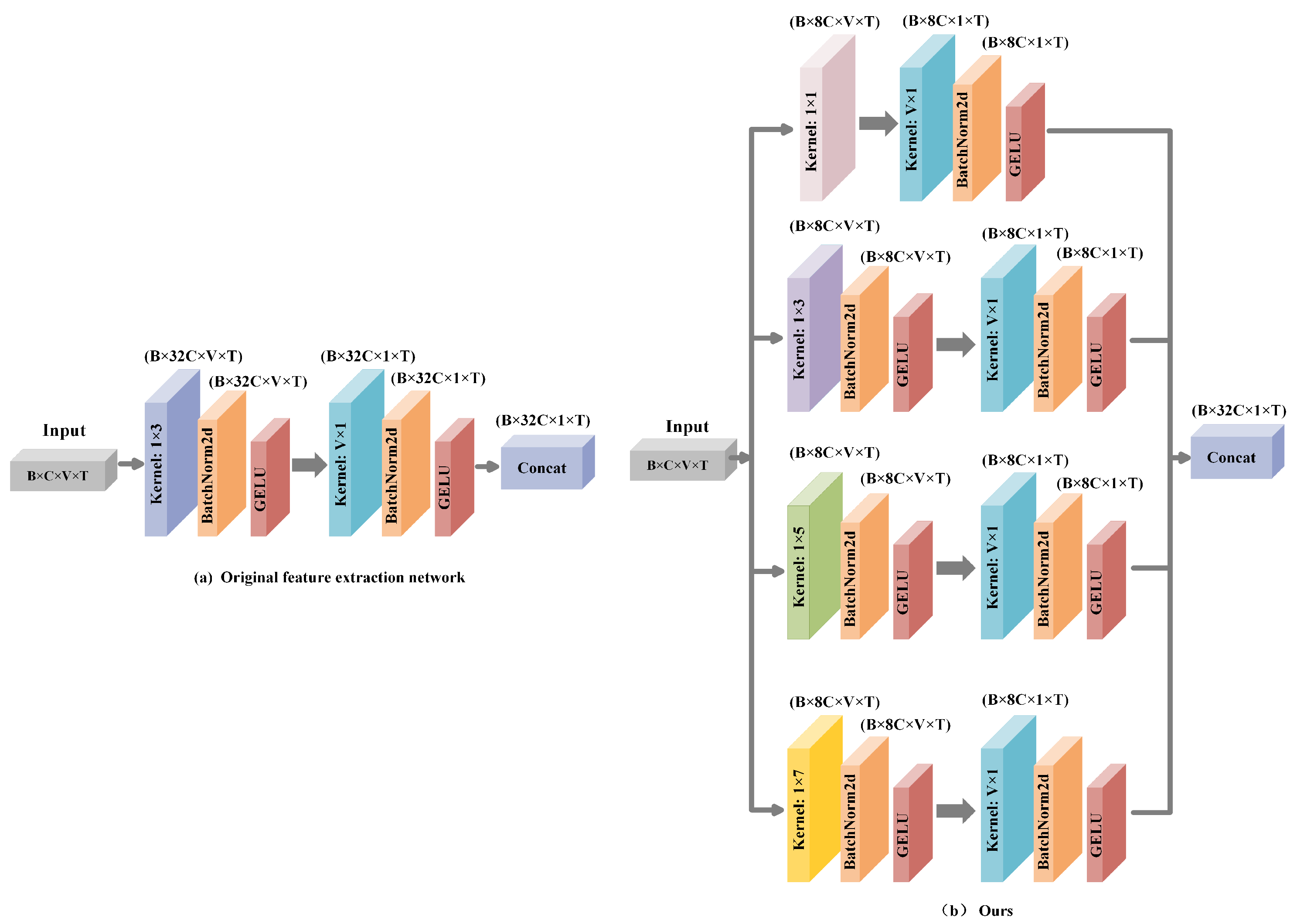

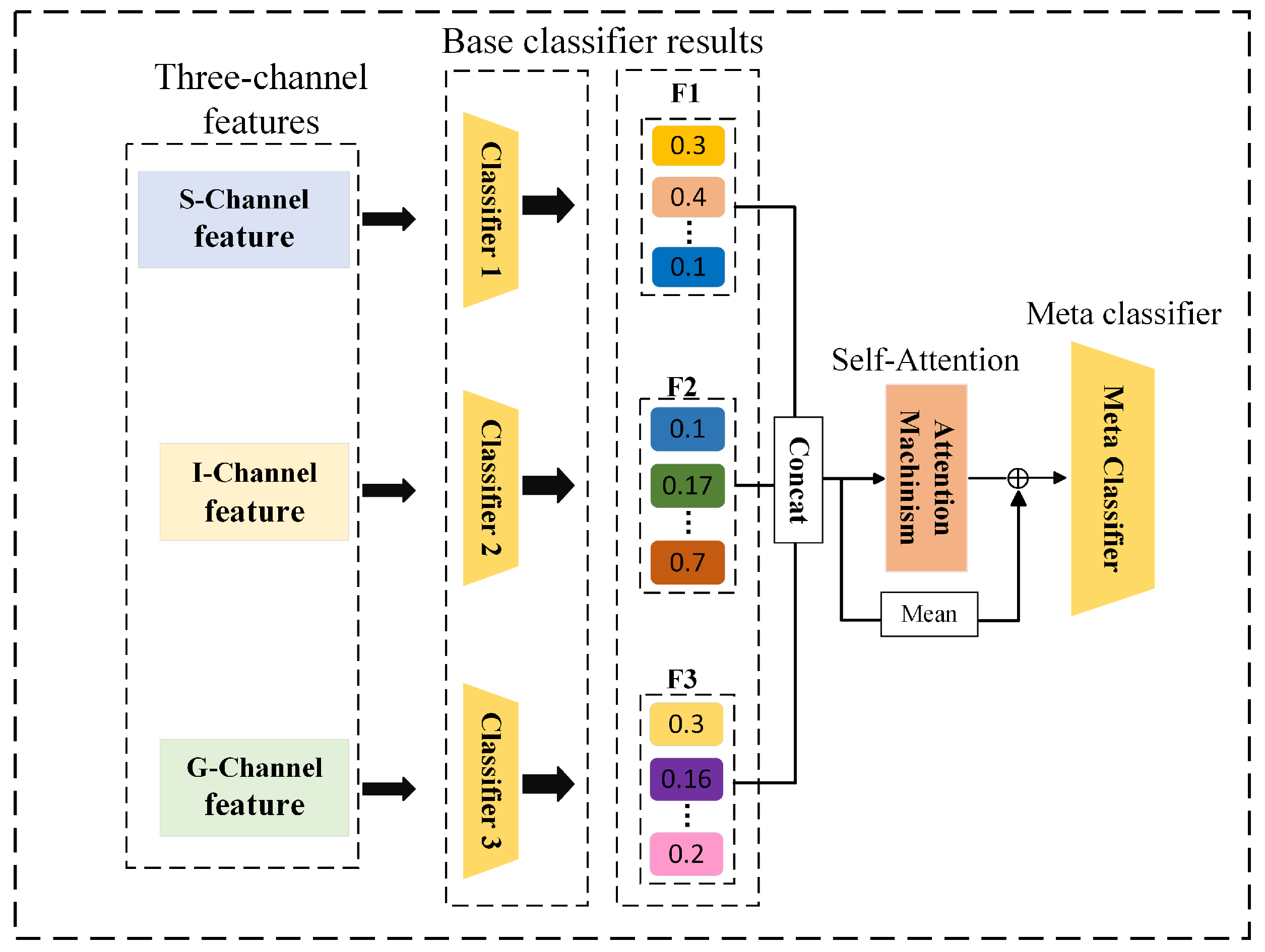
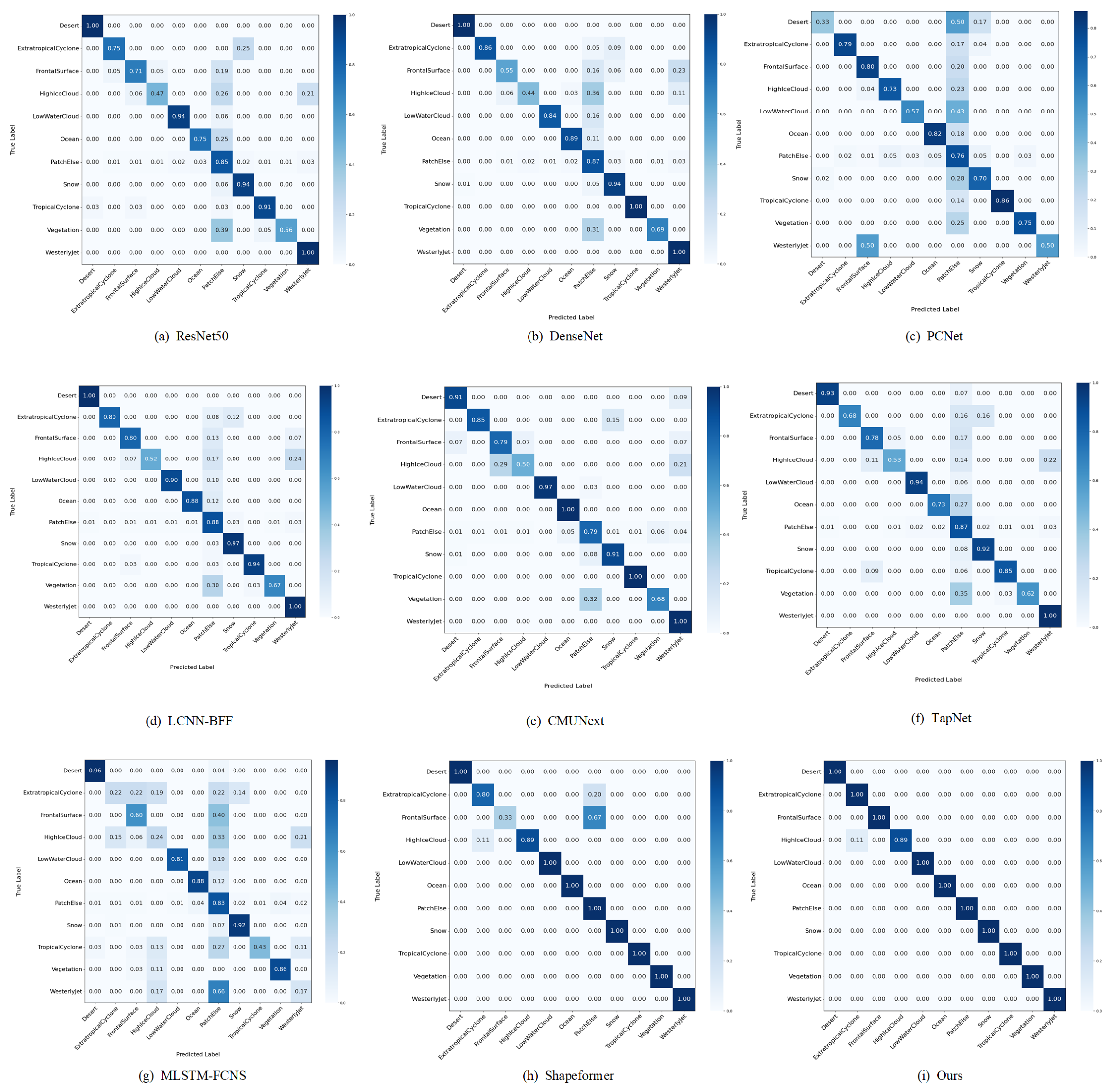
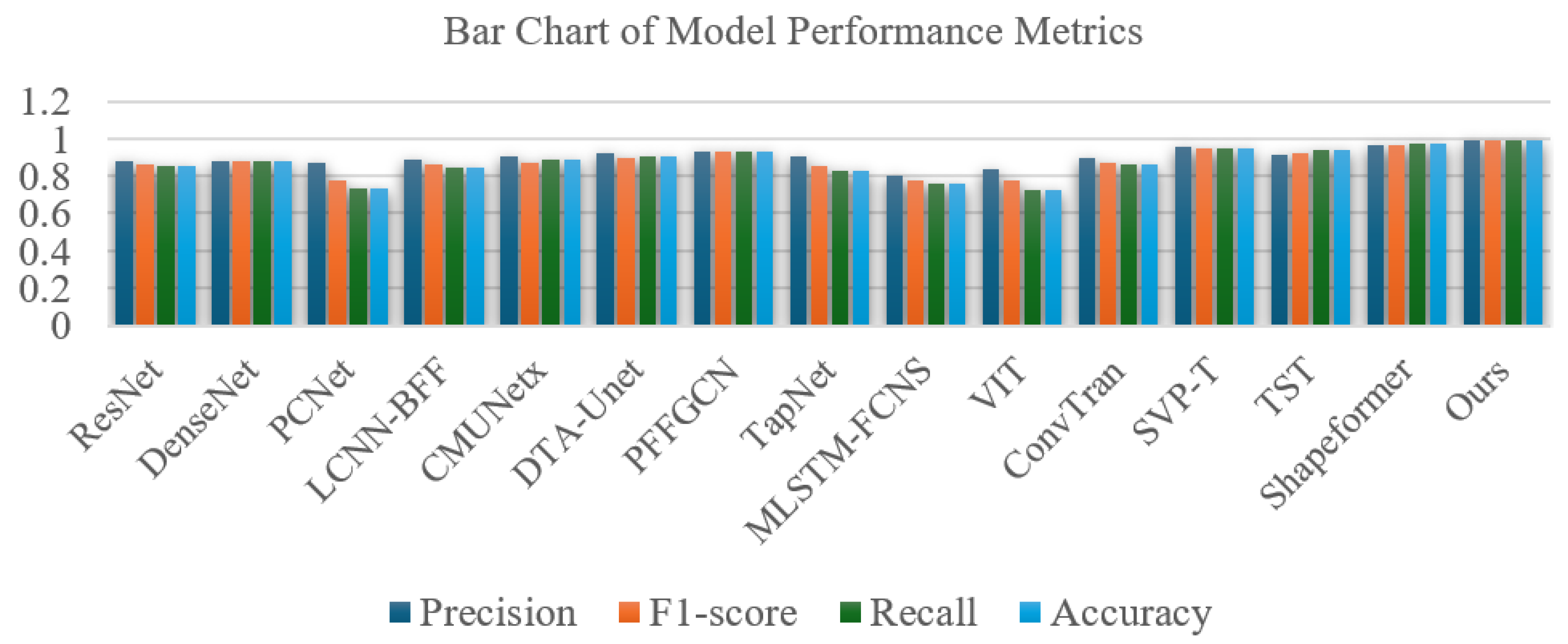
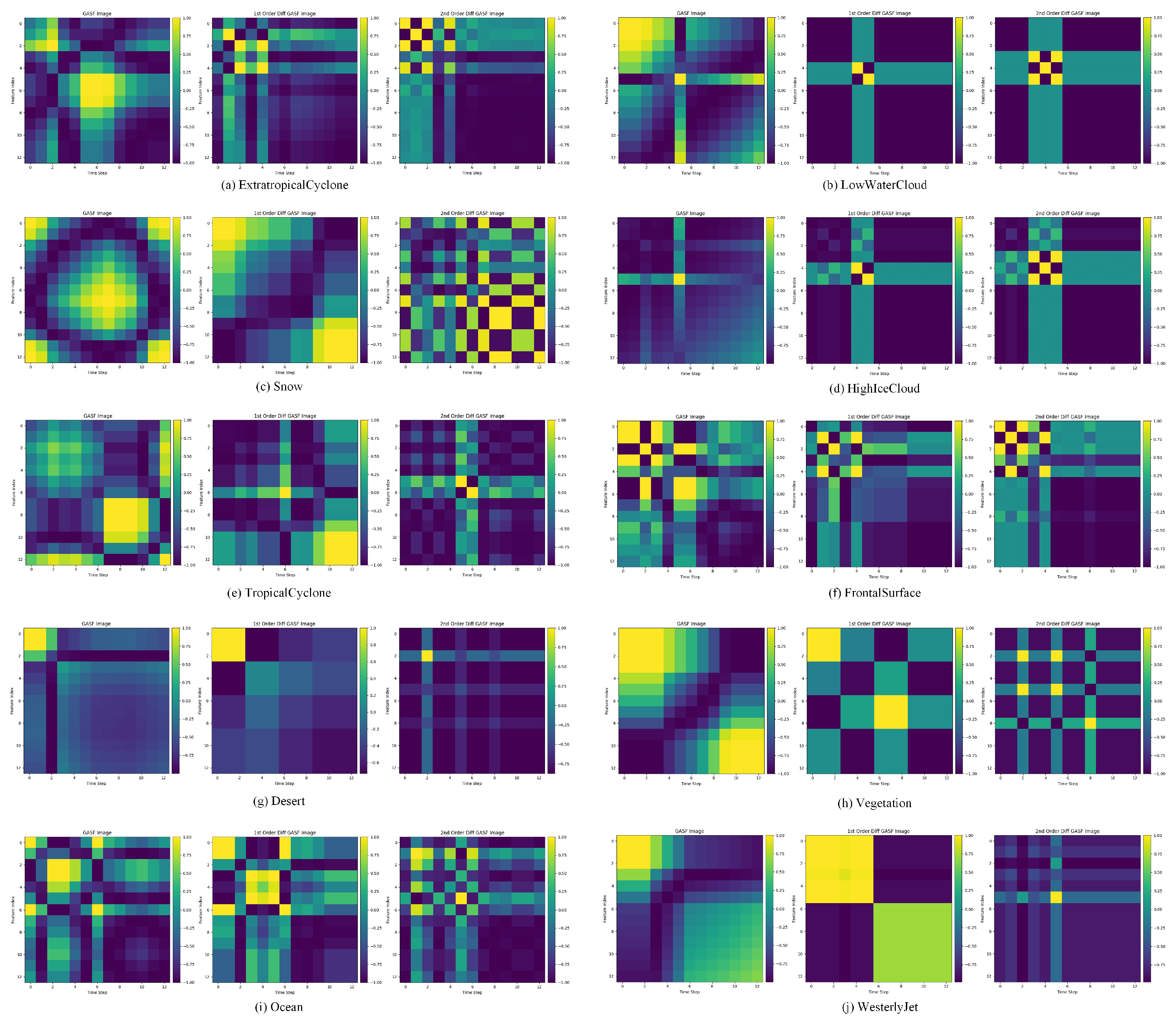
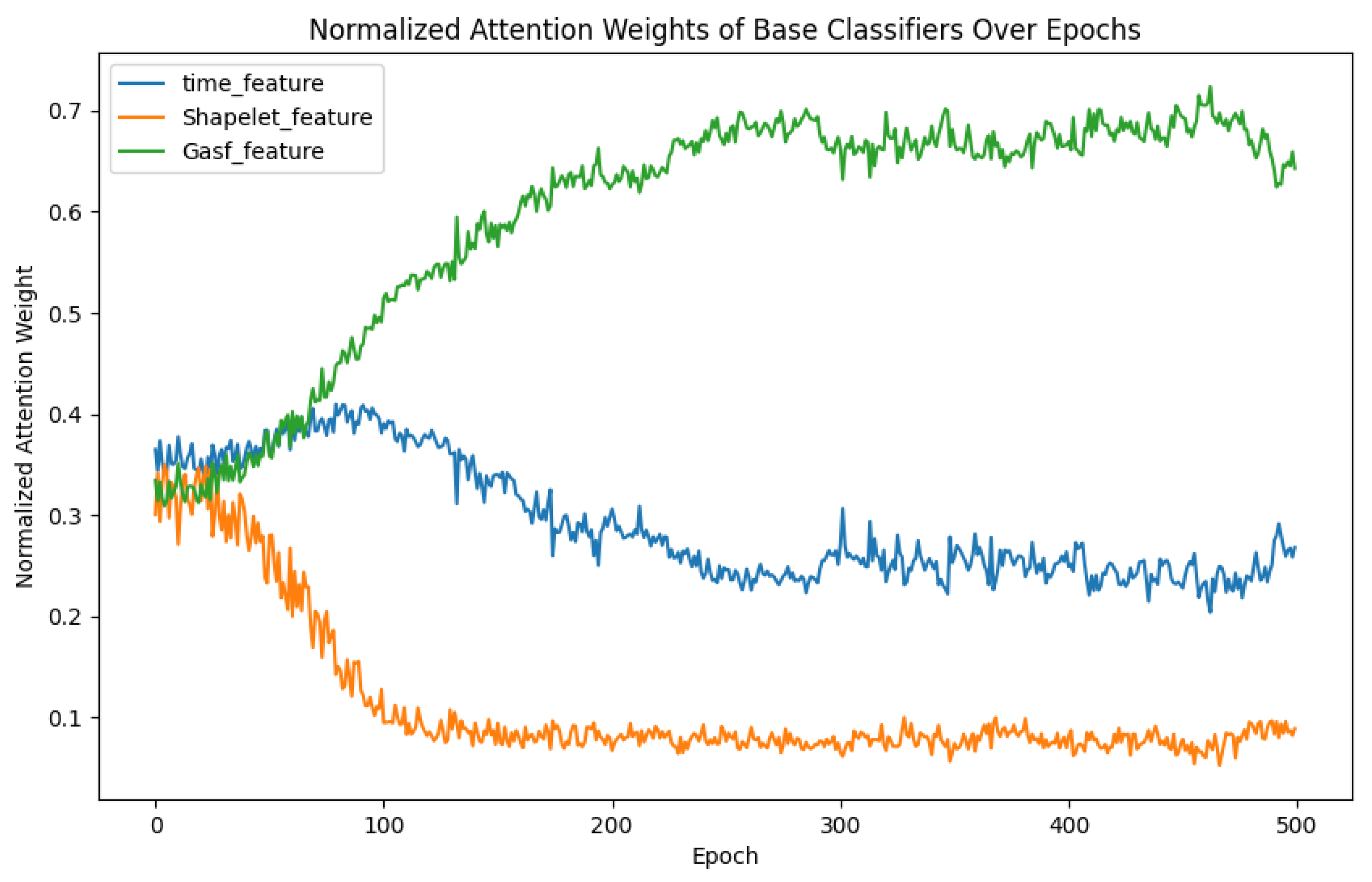
Disclaimer/Publisher’s Note: The statements, opinions and data contained in all publications are solely those of the individual author(s) and contributor(s) and not of MDPI and/or the editor(s). MDPI and/or the editor(s) disclaim responsibility for any injury to people or property resulting from any ideas, methods, instructions or products referred to in the content. |
© 2025 by the authors. Licensee MDPI, Basel, Switzerland. This article is an open access article distributed under the terms and conditions of the Creative Commons Attribution (CC BY) license (https://creativecommons.org/licenses/by/4.0/).