
Accurate Rainfall Prediction Using GNSS PWV Based on Pre-Trained Transformer Model


 , ,
, ,  ,
, 
Abstract
1. Introduction
2. Materials and Methods
2.1. ERA5 Dataset
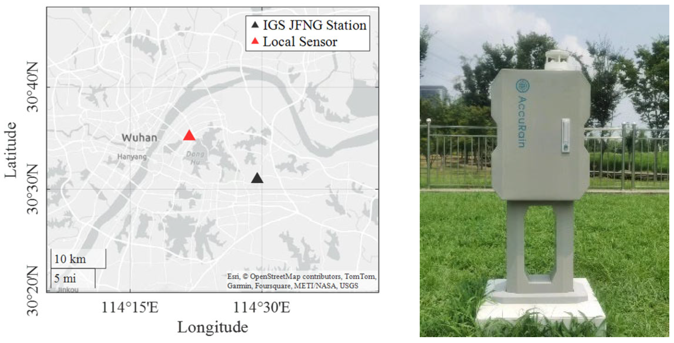
2.2. GNSS Dataset
2.3. PWV Retrieval
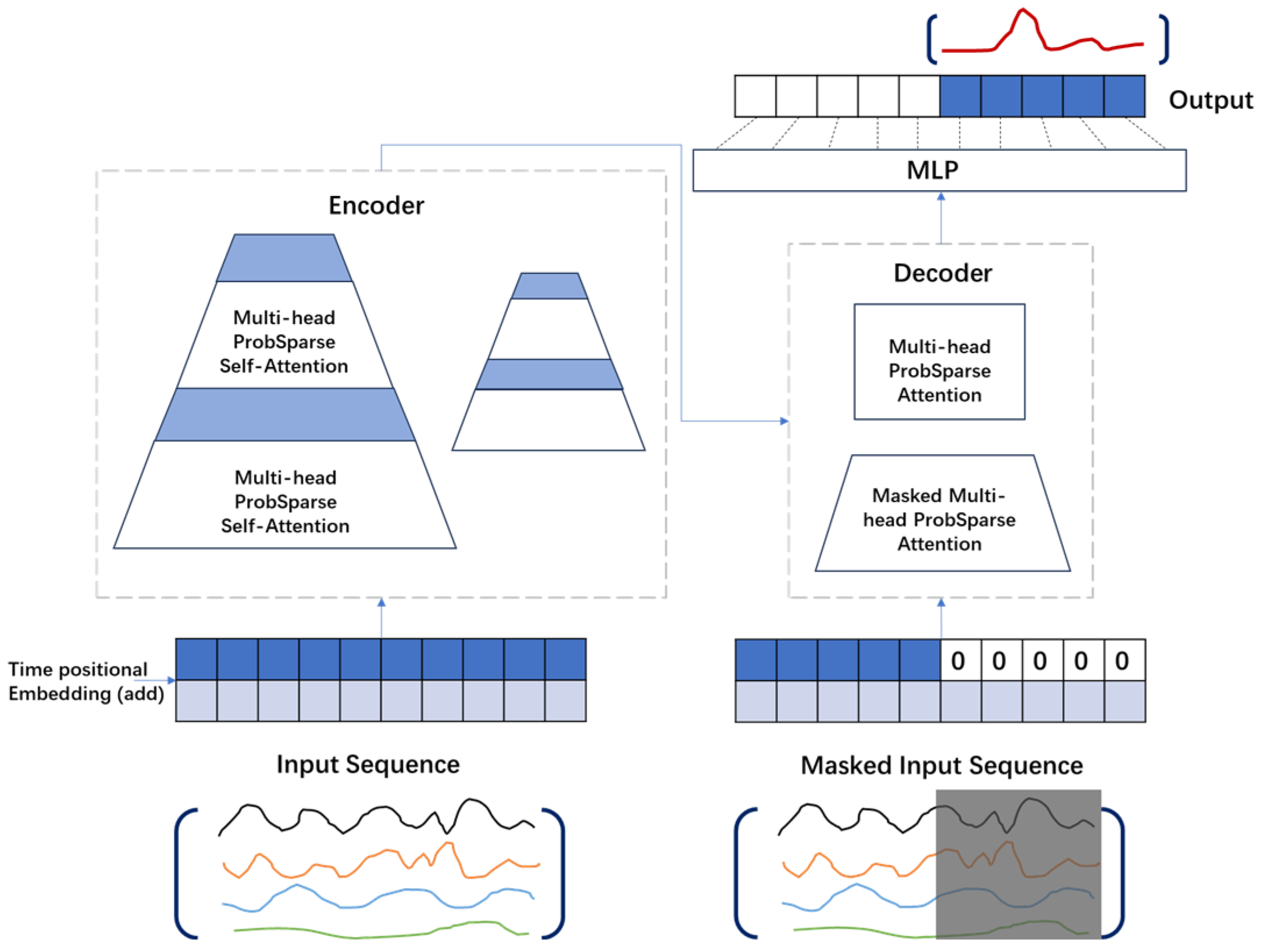
2.4. Model Architecture
2.4.1. Encoder–Decoder Architecture:
2.4.2. Attention Mechanism
2.4.3. Loss Function
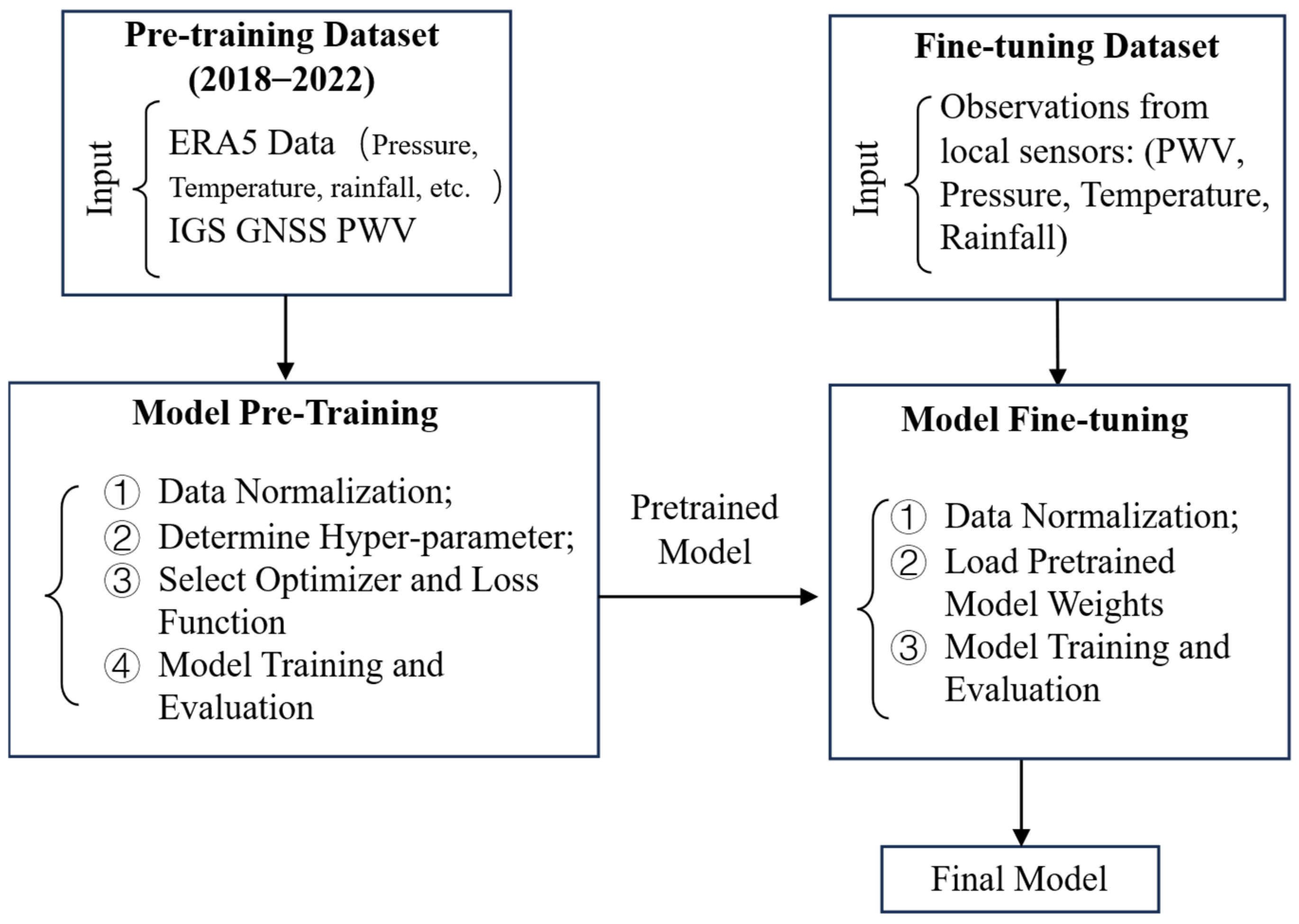
2.5. Model Pre-Training and Fine-Tuning
2.6. Automated Machine Learning (AutoML) Method
2.7. Evaluation Metrics
3. Results
3.1. Experiment Description
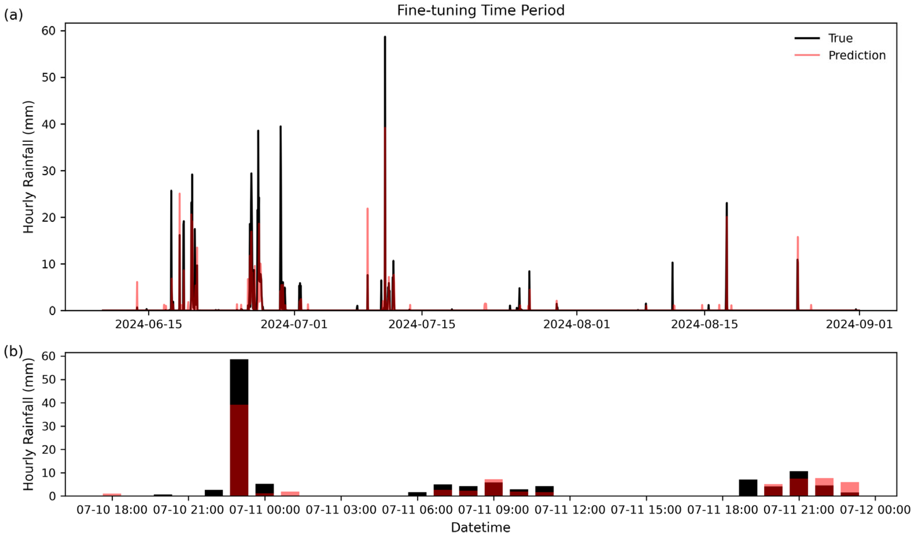
3.2. The Application in Real-Time Nowcasting Experiments
4. Discussion
5. Conclusions
Author Contributions
Funding
Data Availability Statement
Acknowledgments
Conflicts of Interest
Abbreviations
| GNSS | Global Navigation Satellite System |
| PWV | Precipitable water vapor |
| ZTD | Zenith tropospheric delay |
| ZHD | Zenith hydrostatic delay |
| ZWD | Zenith wet delay |
| MSE | Root-mean-square error |
| DTW | Dynamic Time Warping |
| TDI | Time Distortion Index |
| ML | Machine learning |
| AutoML | Automated Machine Learning |
| IGS | International GNSS Service |
References
- Giorgi, F.; Raffaele, F.; Coppola, E. The Response of Precipitation Characteristics to Global Warming from Climate Projections. Earth Syst. Dynam. 2019, 10, 73–89. [Google Scholar] [CrossRef]
- Deng, L.; Feng, J.; Zhao, Y.; Bao, X.; Huang, W.; Hu, H.; Duan, Y. The Remote Effect of Binary Typhoon Infa and Cempaka on the “21.7” Heavy Rainfall in Henan Province, China. J. Geophys. Res. Atmos. 2022, 127, e2021JD036260. [Google Scholar] [CrossRef]
- Trenberth, K.E.; Dai, A.; Rasmussen, R.M.; Parsons, D.B. The Changing Character of Precipitation. Bull. Am. Meteorol. Soc. 2003, 84, 1205–1218. [Google Scholar] [CrossRef]
- Breugem, A.J.; Wesseling, J.G.; Oostindie, K.; Ritsema, C.J. Meteorological Aspects of Heavy Precipitation in Relation to Floods–An Overview. Earth-Sci. Rev. 2020, 204, 103171. [Google Scholar] [CrossRef]
- Liu, Y.; Yao, Y.; Zhao, Q. Real-Time Rainfall Nowcast Model by Combining CAPE and GNSS Observations. IEEE Trans. Geosci. Remote Sens. 2022, 60, 1–9. [Google Scholar] [CrossRef]
- Li, H.; Wang, X.; Choy, S.; Jiang, C.; Wu, S.; Zhang, J.; Qiu, C.; Zhou, K.; Li, L.; Fu, E.; et al. Detecting Heavy Rainfall Using Anomaly-Based Percentile Thresholds of Predictors Derived from GNSS-PWV. Atmos. Res. 2022, 265, 105912. [Google Scholar] [CrossRef]
- Zhang, Y.; Long, M.; Chen, K.; Xing, L.; Jin, R.; Jordan, M.I.; Wang, J. Skilful Nowcasting of Extreme Precipitation with NowcastNet. Nature 2023, 619, 526–532. [Google Scholar] [CrossRef] [PubMed]
- Li, H.; Wang, X.; Wu, S.; Zhang, K.; Chen, X.; Zhang, J.; Qiu, C.; Zhang, S.; Li, L. An Improved Model for Detecting Heavy Precipitation Using GNSS-Derived Zenith Total Delay Measurements. IEEE J. Sel. Top. Appl. Earth Obs. Remote Sens. 2021, 14, 5392–5405. [Google Scholar] [CrossRef]
- Ramezani Ziarani, M.; Bookhagen, B.; Schmidt, T.; Wickert, J.; De La Torre, A.; Deng, Z.; Calori, A. A Model for the Relationship between Rainfall, GNSS-Derived Integrated Water Vapour, and CAPE in the Eastern Central Andes. Remote Sens. 2021, 13, 3788. [Google Scholar] [CrossRef]
- Zhao, Q.; Zhang, X.; Wu, K.; Liu, Y.; Li, Z.; Shi, Y. Comprehensive Precipitable Water Vapor Retrieval and Application Platform Based on Various Water Vapor Detection Techniques. Remote Sens. 2022, 14, 2507. [Google Scholar] [CrossRef]
- Graffigna, V.; Hernández-Pajares, M.; Azpilicueta, F.; Gende, M. Comprehensive Study on the Tropospheric Wet Delay and Horizontal Gradients during a Severe Weather Event. Remote Sens. 2022, 14, 888. [Google Scholar] [CrossRef]
- Li, L.; Zhang, K.; Wu, S.; Li, H.; Wang, X.; Hu, A.; Li, W.; Fu, E.; Zhang, M.; Shen, Z. An Improved Method for Rainfall Forecast Based on GNSS-PWV. Remote Sens. 2022, 14, 4280. [Google Scholar] [CrossRef]
- Schneider, T.; O’Gorman, P.A.; Levine, X.J. Water Vapor and the Dynamics of Climate Changes. Rev. Geophys. 2010, 48, RG3001. [Google Scholar] [CrossRef]
- Du, H.; Donat, M.G.; Zong, S.; Alexander, L.V.; Manzanas, R.; Kruger, A.; Choi, G.; Salinger, J.; He, H.S.; Li, M.-H.; et al. Extreme Precipitation on Consecutive Days Occurs More Often in a Warming Climate. Bull. Am. Meteorol. Soc. 2022, 103, E1130–E1145. [Google Scholar] [CrossRef]
- Valenzuela, R.A.; Garreaud, R.D. Extreme Daily Rainfall in Central-Southern Chile and Its Relationship with Low-Level Horizontal Water Vapor Fluxes. J. Hydrometeorol. 2019, 20, 1829–1850. [Google Scholar] [CrossRef]
- Van Baelen, J.; Reverdy, M.; Tridon, F.; Labbouz, L.; Dick, G.; Bender, M.; Hagen, M. On the Relationship between Water Vapour Field Evolution and the Life Cycle of Precipitation Systems: Evolution of Water Vapour and Precipitation Systems. Q.J.R. Meteorol. Soc. 2011, 137, 204–223. [Google Scholar] [CrossRef]
- Kunkel, K.E.; Stevens, S.E.; Stevens, L.E.; Karl, T.R. Observed Climatological Relationships of Extreme Daily Precipitation Events with Precipitable Water and Vertical Velocity in the Contiguous United States. Geophys. Res. Lett. 2020, 47, e2019GL086721. [Google Scholar] [CrossRef]
- Liu, Z.; Wong, M.S.; Nichol, J.; Chan, P.W. A Multi-sensor Study of Water Vapour from Radiosonde, MODIS and AERONET: A Case Study of Hong Kong. Intl. J. Climatol. 2013, 33, 109–120. [Google Scholar] [CrossRef]
- Niell, A.E.; Coster, A.J.; Solheim, F.S.; Mendes, V.B.; Toor, P.C.; Langley, R.B.; Upham, C.A. Comparison of Measurements of Atmospheric Wet Delay by Radiosonde, Water Vapor Radiometer, GPS, and VLBI. Int. J. Atmos. Ocean. Technol. 2001, 18, 830–850. [Google Scholar] [CrossRef]
- Ferreira, A.P.; Nieto, R.; Gimeno, L. Completeness of Radiosonde Humidity Observations Based on the Integrated Global Radiosonde Archive. Earth Syst. Sci. Data 2019, 11, 603–627. [Google Scholar] [CrossRef]
- Liu, H.; Tang, S.; Zhang, S.; Hu, J. Evaluation of MODIS Water Vapour Products over China Using Radiosonde Data. Int. J. Remote Sens. 2015, 36, 680–690. [Google Scholar] [CrossRef]
- Bevis, M.; Businger, S.; Herring, T.A.; Rocken, C.; Anthes, R.A.; Ware, R.H. GPS Meteorology: Remote Sensing of Atmospheric Water Vapor Using the Global Positioning System. J. Geophys. Res. 1992, 97, 15787–15801. [Google Scholar] [CrossRef]
- Bevis, M.; Businger, S.; Chiswell, S.; Herring, T.A.; Anthes, R.A.; Rocken, C.; Ware, R.H. GPS Meteorology: Mapping Zenith Wet Delays onto Precipitable Water. J. Appl. Meteor. 1994, 33, 379–386. [Google Scholar] [CrossRef]
- Naha Biswas, A.; Lee, Y.H.; Tao Yeo, W.; Low, W.C.; Heh, D.Y.; Manandhar, S. Statistical Analysis of Atmospheric Delay Gradient and Rainfall Prediction in a Tropical Region. Remote Sens. 2024, 16, 4165. [Google Scholar] [CrossRef]
- Rohm, W.; Guzikowski, J.; Wilgan, K.; Kryza, M. 4DVAR Assimilation of GNSS Zenith Path Delays and Precipitable Water into a Numerical Weather Prediction Model WRF. Atmos. Meas. Tech. 2019, 12, 345–361. [Google Scholar] [CrossRef]
- De Pondeca, M.; Zou, X. A Case Study of the Variational Assimilation of GPS Zenith Delay Observations into a Mesoscale Model. J. Appl. Meteorol. 2001, 40, 1559–1576. [Google Scholar] [CrossRef]
- Kawabata, T.; Kuroda, T.; Seko, H.; Saito, K. A Cloud-Resolving 4DVAR Assimilation Experiment for a Local Heavy Rainfall Event in the Tokyo Metropolitan Area. Mon. Weather. Rev. 2011, 139, 1911–1931. [Google Scholar] [CrossRef]
- Zhao, Q.; Liu, Y.; Yao, W.; Yao, Y. Hourly Rainfall Forecast Model Using Supervised Learning Algorithm. IEEE Trans. Geosci. Remote Sens. 2022, 60, 1–9. [Google Scholar] [CrossRef]
- Wu, F.; Zhang, K.; Zhao, J.; Jin, Y.; Li, D. Linear and Nonlinear GNSS PWV Features for Heavy Rainfall Forecasting. Adv. Space Res. 2023, 72, 2170–2184. [Google Scholar] [CrossRef]
- Benevides, P.; Catalao, J.; Nico, G. Neural Network Approach to Forecast Hourly Intense Rainfall Using GNSS Precipitable Water Vapor and Meteorological Sensors. Remote Sens. 2019, 11, 966. [Google Scholar] [CrossRef]
- Benevides, P.; Catalao, J.; Miranda, P.M.A. On the Inclusion of GPS Precipitable Water Vapour in the Nowcasting of Rainfall. Nat. Hazards Earth Syst. Sci. 2015, 15, 2605–2616. [Google Scholar] [CrossRef]
- Liu, Y.; Yao, Y.; Zhao, Q.; Li, Z. Stratified Rainfall Forecast Method Using GNSS Observations. Atmos. Res. 2022, 280, 106421. [Google Scholar] [CrossRef]
- Li, H.; Wang, X.; Wu, S.; Zhang, K.; Fu, E.; Xu, Y.; Qiu, C.; Zhang, J.; Li, L. A New Method for Determining an Optimal Diurnal Threshold of GNSS Precipitable Water Vapor for Precipitation Forecasting. Remote Sens. 2021, 13, 1390. [Google Scholar] [CrossRef]
- Zhao, Q.; Liu, Y.; Ma, X.; Yao, W.; Yao, Y.; Li, X. An Improved Rainfall Forecasting Model Based on GNSS Observations. IEEE Trans. Geosci. Remote Sens. 2020, 58, 4891–4900. [Google Scholar] [CrossRef]
- Liu, Y.; Zhao, Q.; Yao, W.; Ma, X.; Yao, Y.; Liu, L. Short-Term Rainfall Forecast Model Based on the Improved BP–NN Algorithm. Sci. Rep. 2019, 9, 19751. [Google Scholar] [CrossRef] [PubMed]
- Almonacid-Olleros, G.; Almonacid, G.; Gil, D.; Medina-Quero, J. Evaluation of Transfer Learning and Fine-Tuning to Nowcast Energy Generation of Photovoltaic Systems in Different Climates. Sustainability 2022, 14, 3092. [Google Scholar] [CrossRef]
- Rasp, S.; Thuerey, N. Data-Driven Medium-Range Weather Prediction with a Resnet Pretrained on Climate Simulations: A New Model for WeatherBench. J. Adv. Model Earth Syst. 2021, 13, e2020MS002405. [Google Scholar] [CrossRef]
- Bodnar, C.; Bruinsma, W.P.; Lucic, A.; Stanley, M.; Allen, A.; Brandstetter, J.; Garvan, P.; Riechert, M.; Weyn, J.A.; Dong, H.; et al. A Foundation Model for the Earth System. Nature 2025, 641, 1180–1187. [Google Scholar] [CrossRef]
- Muñoz Sabater, J. ERA5-Land Hourly Data from 1950 to Present; Copernicus Climate Change Service (C3S) Climate Data Store (CDS): Reading, UK, 2019. [Google Scholar] [CrossRef]
- Muñoz-Sabater, J.; Dutra, E.; Agustí-Panareda, A.; Albergel, C.; Arduini, G.; Balsamo, G.; Boussetta, S.; Choulga, M.; Harrigan, S.; Hersbach, H.; et al. ERA5-Land: A State-of-the-Art Global Reanalysis Dataset for Land Applications. Earth Syst. Sci. Data 2021, 13, 4349–4383. [Google Scholar] [CrossRef]
- Saastamoinen, J. Atmospheric Correction for the Troposphere and Stratosphere in Radio Ranging Satellites. In Geophysical Monograph Series; Henriksen, S.W., Mancini, A., Chovitz, B.H., Eds.; American Geophysical Union: Washington, DC, USA, 2013; pp. 247–251. ISBN 978-1-118-66364-6. [Google Scholar]
- Takasu, T.; Yasuda, A. Development of the Low-Cost RTK-GPS Receiver with an Open Source Program Package RTKLIB. In Proceedings of the International Symposium on GPS/GNSS 2009, Jeju, Republic of Korea, 4–6 November 2009. [Google Scholar]
- Zhou, H.; Zhang, S.; Peng, J.; Zhang, S.; Li, J.; Xiong, H.; Zhang, W. Informer: Beyond Efficient Transformer for Long Sequence Time-Series Forecasting. In Proceedings of the AAAI Conference on Artificial Intelligence, 2–9 February 2021; AAAI Press: Palo Alto, CA, USA, 2021; pp. 11106–11115. [Google Scholar]
- Vaswani, A.; Shazeer, N.; Parmar, N.; Uszkoreit, J.; Jones, L.; Gomez, A.N.; Kaiser, Ł.; Polosukhin, I. Attention Is All You Need. In Proceedings of the Advances in Neural Information Processing Systems; Guyon, I., Luxburg, U.V., Bengio, S., Wallach, H., Fergus, R., Vishwanathan, S., Garnett, R., Eds.; Curran Associates, Inc.: Red Hook, NY, USA, 2017; Volume 30. [Google Scholar]
- Le Guen, V.; Thome, N. Deep Time Series Forecasting with Shape and Temporal Criteria. IEEE Trans. Pattern Anal. Mach. Intell. 2023, 45, 342–355. [Google Scholar] [CrossRef]
- Sakoe, H.; Chiba, S. Dynamic Programming Algorithm Optimization for Spoken Word Recognition. IEEE Trans. Acoust. Speech Signal Process. 1978, 26, 43–49. [Google Scholar] [CrossRef]
- Vallance, L.; Charbonnier, B.; Paul, N.; Dubost, S.; Blanc, P. Towards a Standardized Procedure to Assess Solar Forecast Accuracy: A New Ramp and Time Alignment Metric. Sol. Energy 2017, 150, 408–422. [Google Scholar] [CrossRef]
- Shi, J.; Shirali, A.; Jin, B.; Zhou, S.; Hu, W.; Rangaraj, R.; Wang, S.; Han, J.; Wang, Z.; Lall, U.; et al. Deep Learning and Foundation Models for Weather Prediction: A Survey 2025. arXiv 2025, arXiv:2501.06907. [Google Scholar]
- Wang, C.; Wu, Q.; Weimer, M.; Zhu, E. FLAML: A Fast and Lightweight AutoML Library. In Proceedings of the Machine Learning and Systems, Stanford, CA, USA, 31 March–2 April 2019. [Google Scholar] [CrossRef]
- Chen, T.; Guestrin, C. XGBoost: A Scalable Tree Boosting System. In Proceedings of the 22nd ACM SIGKDD International Conference on Knowledge Discovery and Data Mining, San Francisco, CA, USA, 13–17 August 2016. [Google Scholar]
- Meng, Q. LightGBM: A Highly Efficient Gradient Boosting Decision Tree. In Proceedings of the Neural Information Processing Systems, Long Beach, CA, USA, 4–9 December 2017. [Google Scholar]
- Kunkel, K.E.; Karl, T.R.; Squires, M.F.; Yin, X.; Stegall, S.T.; Easterling, D.R. Precipitation Extremes: Trends and Relationships with Average Precipitation and Precipitable Water in the Contiguous United States. J. Appl. Meteorol. Climatol. 2020, 59, 125–142. [Google Scholar] [CrossRef]
- Poelzl, M.; Kern, R.; Kecorius, S.; Lovrić, M. Exploration of Transfer Learning Techniques for the Prediction of PM10. Sci. Rep. 2025, 15, 2919. [Google Scholar] [CrossRef]

| Metric | Description |
|---|---|
| MSE | Mean square error |
| DTW | Dynamic Time Warping |
| TDI | Time Distortion Index |
| Parameters | Sequence Length | Label Length | Batch Size | Learning Rate | Encoder Layers | Decoder Layers | |
|---|---|---|---|---|---|---|---|
| Schemes | |||||||
| Scheme 1 | 48 | 48 | 64 | 5 × 10⁻⁵ | 3 | 3 | |
| Scheme 2 | 48 | 24 | 64 | 5 × 10⁻⁵ | 3 | 3 | |
| Scheme 3 | 24 | 12 | 64 | 5 × 10⁻⁵ | 3 | 3 | |
| Scheme 4 | 12 | 6 | 64 | 5 × 10⁻⁵ | 3 | 3 | |
| Scheme 5 | 72 | 48 | 64 | 5 × 10⁻⁵ | 3 | 3 | |
| Scheme 6 | 96 | 48 | 64 | 5 × 10⁻⁵ | 3 | 3 | |
| Models | Scheme 1 | Scheme 2 | Scheme 3 | Scheme 4 | Scheme 5 | Scheme 6 | |
|---|---|---|---|---|---|---|---|
| Metric | |||||||
| MSE | 0.368 | 0.214 | 0.403 | 0.263 | 0.361 | 0.483 | |
| DTW | 0.032 | 0.019 | 0.071 | 0.030 | 0.061 | 0.097 | |
| TDI | 0.208 | 0.206 | 0.076 | 0.195 | 0.078 | 0.118 | |
| Models | Pre-Trained Model | Fine-Tuned Model | Model Trained from Scratch | AutoML | |
|---|---|---|---|---|---|
| Metric | |||||
| MSE | 6.212 | 3.954 | 4.295 | 5.869 | |
| DTW | 1.113 | 0.232 | 0.205 | 2.661 | |
| TDI | 0.136 | 0.101 | 0.171 | 0.114 | |
Disclaimer/Publisher’s Note: The statements, opinions and data contained in all publications are solely those of the individual author(s) and contributor(s) and not of MDPI and/or the editor(s). MDPI and/or the editor(s) disclaim responsibility for any injury to people or property resulting from any ideas, methods, instructions or products referred to in the content. |
© 2025 by the authors. Licensee MDPI, Basel, Switzerland. This article is an open access article distributed under the terms and conditions of the Creative Commons Attribution (CC BY) license (https://creativecommons.org/licenses/by/4.0/).
Share and Cite
Yin, W.; Zhou, C.; Tian, Y.; Qiu, H.; Zhang, W.; Chen, H.; Liu, P.; Zhao, Q.; Kong, J.; Yao, Y. Accurate Rainfall Prediction Using GNSS PWV Based on Pre-Trained Transformer Model. Remote Sens. 2025, 17, 2023. https://doi.org/10.3390/rs17122023
Yin W, Zhou C, Tian Y, Qiu H, Zhang W, Chen H, Liu P, Zhao Q, Kong J, Yao Y. Accurate Rainfall Prediction Using GNSS PWV Based on Pre-Trained Transformer Model. Remote Sensing. 2025; 17(12):2023. https://doi.org/10.3390/rs17122023
Chicago/Turabian StyleYin, Wenjie, Chen Zhou, Yuan Tian, Hui Qiu, Wei Zhang, Hua Chen, Pan Liu, Qile Zhao, Jian Kong, and Yibin Yao. 2025. "Accurate Rainfall Prediction Using GNSS PWV Based on Pre-Trained Transformer Model" Remote Sensing 17, no. 12: 2023. https://doi.org/10.3390/rs17122023
APA StyleYin, W., Zhou, C., Tian, Y., Qiu, H., Zhang, W., Chen, H., Liu, P., Zhao, Q., Kong, J., & Yao, Y. (2025). Accurate Rainfall Prediction Using GNSS PWV Based on Pre-Trained Transformer Model. Remote Sensing, 17(12), 2023. https://doi.org/10.3390/rs17122023