Extraction of Suaeda salsa from UAV Imagery Assisted by Adaptive Capture of Contextual Information

Abstract

Suaeda salsa, a halophytic plant species, exhibits a remarkable salt tolerance and demonstrates a significant phytoremediation potential through its capacity to absorb and accumulate saline ions and heavy metals from soil substrates, thereby contributing to soil quality amelioration. Furthermore, this species serves as a critical habitat component for avifauna populations and represents a keystone species in maintaining ecological stability within estuarine and coastal wetland ecosystems. With the development and maturity of UAV remote sensing technology in recent years, the advantages of using UAV imagery to extract weak targets are becoming more and more obvious. In this paper, for Suaeda salsa, which is a weak target with a sparse distribution and inconspicuous features, relying on the high-resolution and spatial information-rich features of UAV imagery, we establish an adaptive contextual information extraction deep learning semantic segment model (ACI-Unet), which can solve the problem of recognizing Suaeda salsa from high-precision UAV imagery. The precise extraction of Suaeda salsa was completed in the coastal wetland area of Dongying City, Shandong Province, China. This paper achieves the following research results: (1) An Adaptive Context Information Extraction module based on large kernel convolution and an attention mechanism is designed; this module functions as a multi-scale feature extractor without altering the spatial resolution, enabling a seamless integration into diverse network architectures to enhance the context-aware feature representation. (2) The proposed ACI-Unet (Adaptive Context Information U-Net) model achieves a high-precision identification of Suaeda salsa in UAV imagery, demonstrating a robust performance across heterogeneous morphologies, densities, and scales of Suaeda salsa populations. Evaluation metrics including the accuracy, recall, F1 score, and mIou all exceed 90%. (3) Comparative experiments with state-of-the-art semantic segmentation models reveal that our framework significantly improves the extraction accuracy, particularly for low-contrast and diminutive Suaeda salsa targets. The model accurately delineates fine-grained spatial distribution patterns of Suaeda salsa, outperforming existing approaches in capturing ecologically critical structural details.

1. Introduction

As a halophytic species endemic to estuarine and coastal wetlands, Suaeda salsa exhibits an exceptional salt tolerance through evolutionary adaptations to periodic tidal inundation. It can improve the ecological environment of estuarine and coastal wetlands, enhance the biodiversity of this region, and also serves as an important foraging ground and transit station for birds, especially migratory birds. Large-scale Suaeda salsa has formed the unique coastal wetland landscape the “Red Beach”. The “Red Beach” is a famous coastal wetland landscape in China, located at about 37.625°N in Dongying City, ShanDong Province, 118.967°E, which is an ideal place for people to understand coastal wetlands and typical marine ecosystems and experience the charm of the ocean [1,2].

Suaeda salsa, as a common plant in wetlands, is of great significance to the study of wetland ecology and environments. The traditional coastal wetland vegetation research mainly relies on field surveys, which is not only costly, but also relatively limited in scope and time and is relatively inefficient. The use of remote sensing technology for wetland vegetation research not only saves manpower and material resources but also realizes the monitoring of large-scale and long time series. For the extraction of Suaeda salsa on remote sensing images, which is the research object of this paper, many scholars have also conducted research. Li et al. [3] realized the extraction of the spatio-temporal distribution information of the Liaohekou salt flat’s Suaeda salsa from 2017 to 2023 based on multi-temporal Sentinel-2 images using the method of extracting the optimal decision rule from a trained random forest model. Zhang et al. [4] constructed a feature vector set containing phenological, optical, red-edge, and radar features based on Sentinel-1 and Sentinel-2 multi-source remote sensing images and used a random forest algorithm to categorize the wetland plant communities in the Yellow River Delta in 2021. Ke et al. [5] constructed a saline Suaeda salsa spectral index (SSSI) for the extraction of Suaeda salsa in order to refine the extraction and estimation of saline Suaeda salsa. Most of the above studies use medium-resolution images, as shown in Figure 1. Suaeda salsa is a research target with small and weak individual plants and sparse distributions. Affected by the background of tidal flat wetlands, tides, etc., the extraction of Suaeda salsa based on medium- or low-resolution satellite remote sensing images cannot provide a refined spatial distribution result. However, sufficient spatial information can improve the accuracy of extracting such small and weak targets. Therefore, many researchers should use high-resolution images as much as possible to obtain the relevant information of Suaeda salsa. In this regard, many scholars have conducted research. Gao et al. [6] constructed a decision tree based on unmanned aerial hyperspectral imagery, screening sensitive spectral features and vegetation index features of Suaeda salsa, and effectively extracted spatial distribution information of Suaeda salsa in the Yuanyanggou wetland area at the mouth of the Liaohe River. Based on hyperspectral remote sensing images, Ren et al. [7] evaluated the ability of nine commonly used spectral indices to estimate the biomass of HJ-1 hyperspectral reed and Suaeda salsa in the Yellow River estuary and inverted the vegetation species in the Yellow River estuary based on the screened index characteristics combined with the data from the field reconnaissance surveys using a simple linear regression. Du et al. [8] explored the capability of airborne multispectral imagery, satellite hyperspectral imagery, and LiDAR data for Suaeda salsa spatial distribution extraction. Zhang et al. [9,10] simulated the growth cycle of Suaeda salsa and adapted the PROSAIL-D model to better fit the spectral characteristics of Suaeda salsa based on the relationship between the chlorophyll content and betacyanin (Beta) absorption coefficient. Although high-resolution images can overcome the problem of insufficient fine-grained results, the methods of image processing also become complex. Most of the above studies use traditional machine learning methods, which rely on artificially constructed feature sets, and seriously restrict the level and accuracy of the automation.

In recent years, with the development of various deep learning-based computer vision methods, the intelligent extraction of remote sensing information under high resolutions has become a popular research topic. Compared with the traditional remote sensing information extraction methods, deep learning methods do not need to extract additional features, and there is a large increase in accuracy and efficiency, and in terms of the intelligent extraction of information from high-resolution remote sensing imagery, the existing techniques have been relatively mature. Maggiori, Lv, Zhang et al. [11,12,13] used a convolutional neural network (CNN) for high-resolution remote sensing scene classification, and the results showed that the generalization effect from the pre-trained CNN was very good. Li et al. [14] propose a deep learning-based cloud detection method named multi-scale convolutional feature fusion (MSCFF) for remote sensing images of different sensors. The experimental results show that MSCFF achieves a higher accuracy than the traditional rule-based cloud detection methods and the state-of-the-art deep learning models. Hu et al. [15] proposed a multi-branch convolutional attention network MCANet for the segmentation of cloud and snow regions, and the results showed that it outperformed traditional machine learning models and CNN models on two publicly available datasets (HRC_WHU and L8 SPARCS). Fu et al. [16] designed an algorithm based on the DeepLabV3+ multi-scale feature extraction module that fused optical remote sensing imagery and the Digital Elevation Model (DEM) and another multi-source data deep learning model to extract karst landforms in southern China. Most of the deep learning models used in the above studies are based on the Encoder–Decoder framework, which is capable of end-to-end image segmentation and can handle complex information in high-resolution images. Although deep learning methods can effectively process various complex information in high-resolution images, the acquisition cost of high-resolution images is undoubtedly enormous.

In recent years, UAV remote sensing technology has developed rapidly. It has the advantages of a high efficiency, high flexibility, and high cost-effectiveness and has been adopted by more and more researchers. As UAV remote sensing images have become one of the mainstream data sources for target identification and detection [17,18,19,20], how to utilize the rich information from UAV imagery has become a challenge in the current research. Suaeda salsa, influenced by various factors such as the terrain and salinity, exhibits different phenotypes under different growth conditions. These phenotypes are typically manifested in UAV imagery as inconsistent sizes, irregular shapes, and significant color variations, as shown in Figure 1. This phenomenon leads to difficulty in recognizing Suaeda salsa. Usually, the resolution of UAV imagery (especially in spatial resolution) is mostly higher than that of satellite images, and in order to refine the extraction of Suaeda salsa, it is necessary to take advantage of this rich spatial information, and the interference caused by image contextual information has to be taken into account in the design of the model [21]. Based on DeepLabV3, Liu et al. [22] added a jump connection and convolutional layer in the decoder to unite contextual feature information. Zheng et al. [23] designed an STER model for semantic segmentation based on the transform’s decoder, and according to the idea of temporal processing, global contextual information can be fused. Deep learning techniques can effectively utilize the rich information in high-resolution images, but general segmentation models sometimes cannot adapt well to the challenges caused by downstream tasks. In practice, convolutional neural networks obtain contextual information at different scales by adjusting the receptive field size and downsampling. However, these processes can change the resolution of the feature map, leading to information loss. Specifically, for our task, weak targets like Suaeda salsa require both sufficient detail information to display the spatial distribution and attention to contextual information for accurate recognition. This poses a challenge to our task.

To address the difficulties in identifying Suaeda salsa in UAV imagery due to the small target size, inconsistent sizes, irregular shapes, and inconsistent colors, this paper constructs a network called Adaptive Context Information U-Net (ACI-Unet) based on the U-Net (Unet) framework [24] and incorporating an Adaptive Context Information Extraction (ACIE) module. The application of this model has enabled the precise extraction of Suaeda salsa targets from UAV imagery, and the extracted results have been analyzed.

2. Materials and Methods

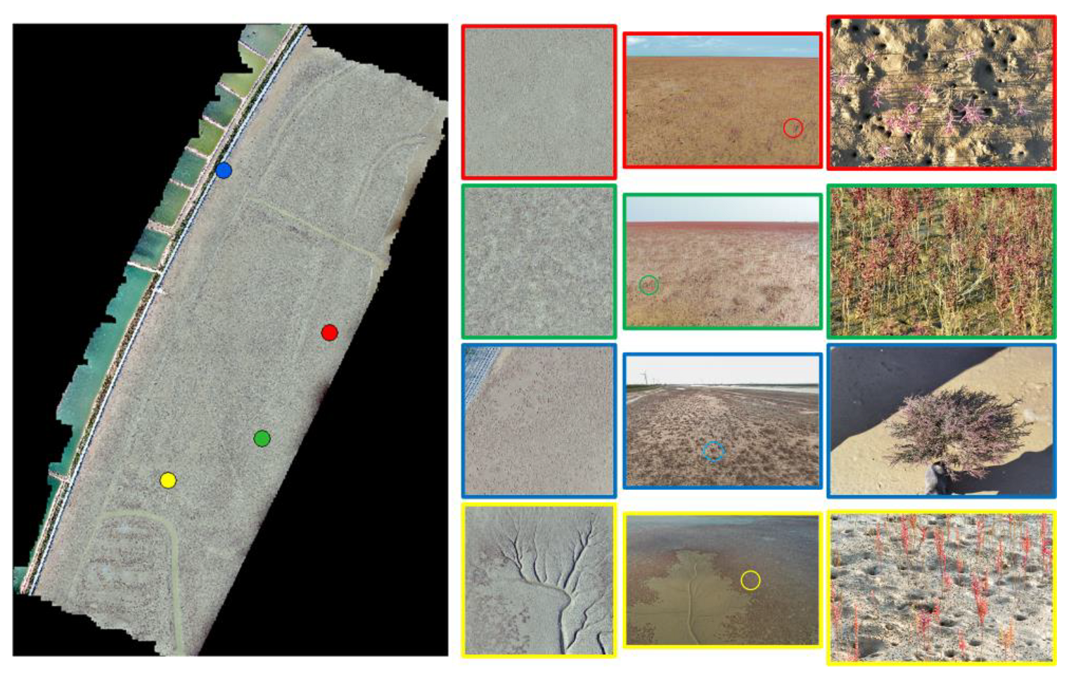
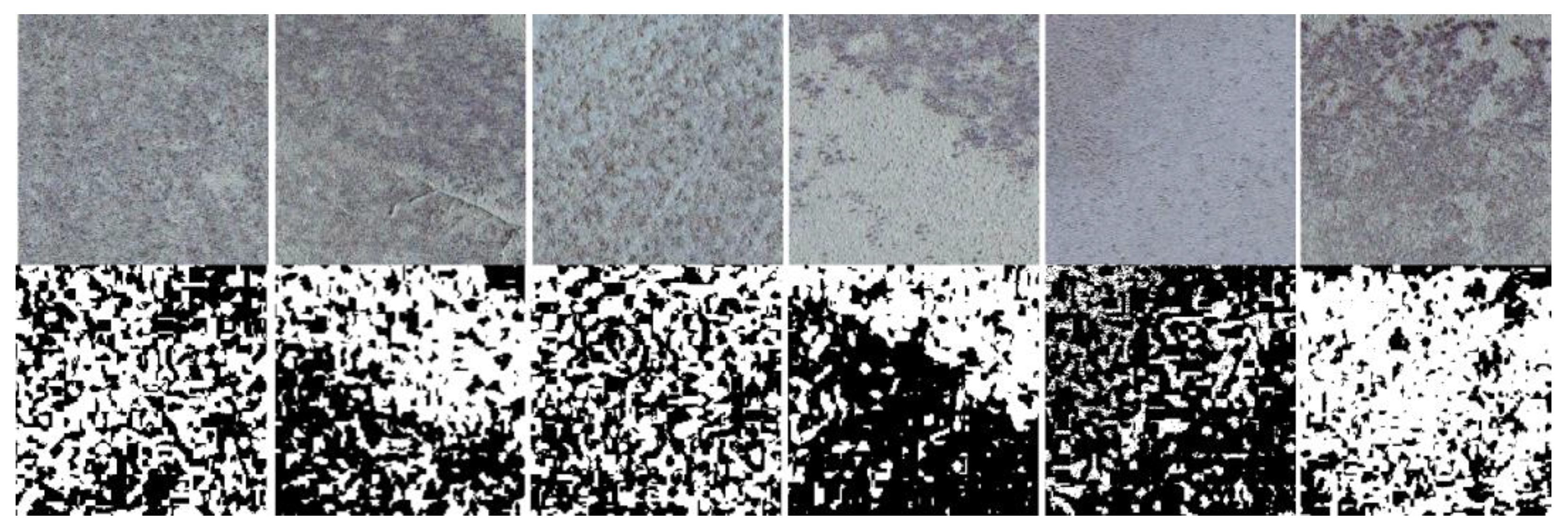
2.1. Dataset Construction

The data used in this experiment is the orthophoto acquired by airborne UAV which made by feima robotics in Beijing china; the spatial resolution is 0.05 m, the image is visible image, shot with RGB camera, the image size is 23,766 × 34,629 after preprocessing, and the map projection is WGS-84. The study area of this paper is located in Dongying City, Shandong Province, China, (Figure 2) where a large number of ecological restoration projects of Suaeda salsa have been carried out in recent years. Since a large amount of labeled data is required to use deep learning models [25], this paper combines the field survey data with visual interpretation to produce sample labels, after which the collected labels are randomly cropped and vertically flipped to generate 673 image pairs of 256 × 256 sizes, and the binarized results are shown in Figure 3, and the training and validation datasets will be finally divided using a ratio of 8:2.

2.2. Context-Adaptive Information Model Construction Based on Encoder–Decoder Framework

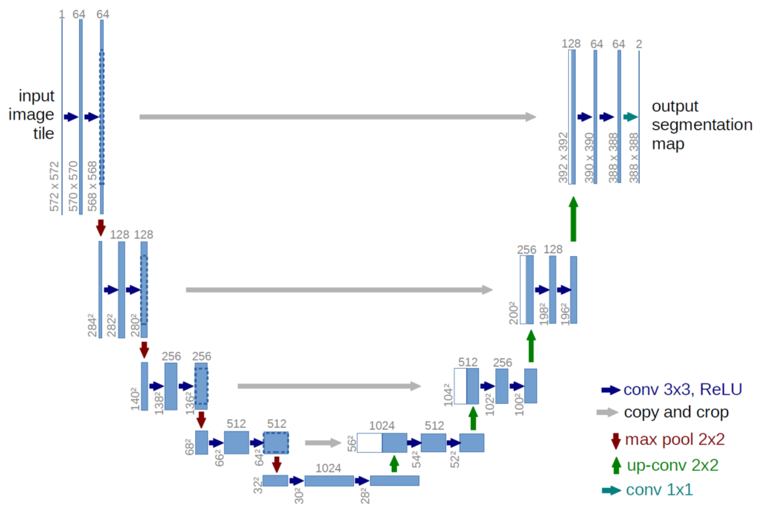
2.2.1. Unet Model

Unet was proposed by Ronneberger et al. in 2015 [24] (Figure 4), which was initially designed for medical image segmentation, but due to its excellent performance, it is now widely used in other fields, such as satellite image processing and cellular image segmentation [26,27,28]. The encoder part of the model gradually extracts image features through multilayer convolution and maximum pooling operations and gradually reduces the spatial dimensions of the feature map; the decoder part gradually recovers the original dimensions of the image through upsampling and convolution. In addition, U-Net introduces jump connections to pass the output in the encoder directly to the decoder through jump links in order to preserve the low-level detail information in the reconstruction process.

2.2.2. ACIE Module

It has been proven that using large kernel convolution to expand the sensory field of the network to obtain target context information is an effective way for image target recognition [26]. However, too many features will bring computational burden and information redundancy to the network. In response to this phenomenon, scholars use the attention mechanism to make the network more focused on useful features and realize adaptive feature extraction [29,30]. Therefore, in this paper, an adaptive contextual information extraction (ACIE) module is designed based on the large kernel convolution and attention mechanism as shown in Figure 5. ACIE overall contains three modules: the large kernel convolution module, the spatial attention module, and the channel attention module. The large kernel convolution is to extract the multi-scale features of the Suaeda salsa, and the spatial and channel attention mechanisms are to adapt different features to the different phenotypes of the Suaeda salsa. The ACIE module performs the two large kernel convolutions first to extract the multi-scale features and then the extracted features through the spatial attention module, which in turn consists of average pooling, maximum pooling, and 7 × 7 convolutional layers. The spatially filtered features are then passed through the channel attention to enhance the characterization ability of the module.

(1)

Large kernel convolutional module

Convolutional neural networks acquire the contextual information of a target through convolutional layers, and usually, multi-scale contextual information can be effectively extracted by expanding the receptive field of the network [31]. In addition, as mentioned earlier, a target such as Suaeda salsa is usually small in size and irregular in shape on the image, and such a target needs to retain as much spatial detail information as possible when extracting contextual information [32]. Therefore, in order to preserve the resolution of the feature map and extract enough context information, we designed two large kernel convolutional layers, f_1 (K = 5, P = 2, S = 1) and f_2 (K = 7, P = 9, S = 1, D = 3), that do not change the size of the feature map. The mathematical computation process is shown in Equations (1) and (2). X is the input feature map, $Y_1$ and $Y_2$ denote the result after convolution operation, H and W denote the dimension size of feature map, and $C_1$ and $C_2$ denote the number of channels after calculation. K is the size of convolution kernel, P is the number of paddings, S is the sliding step size of convolution window, and D is the expansion times of convolution window.

$${Y_1^{C_1\times H\times W}}_{(i,j)}=f_1(X_{(i,j)})$$

(1)

$${Y_2^{C_2\times H\times W}}_{(i,j)}=f_2(Y_{1(i,j)})$$

(2)

(2)

Spatial attention mechanism module

The basic idea of the spatial attention mechanism is to assign different weights to the input feature map based on the spatial location in the image (i.e., each pixel location or region of the image). This design allows the network to focus more on the detailed parts of the image. The spatial attention mechanism used in this study references the Convolutional Block Attention Module (CBAM) designed by Kweon et al. [33]. However, unlike CBAM, we used a convolutional layer with a larger convolutional kernel instead of the original MLP, which can help the network to better focus on the contextual information as well as reduce the computational effort of the network. Specifically, $Y_1$ and $Y_2$ are first through the convolution kernel size 1 × 1 convolution layer $f_{1\times 1}$ for dimensionality reduction. The results of the dimensionality reduction are then stitched together in the channel dimension. After global pixel-level average pooling, $Av{g}_p$ and maximum pooling $Ma{x}_p$, two masks, $m_1$ and $m_2$, with the same size as the feature size are generated, and then two attention mechanism masks, $M_1$ and $M_2$, are generated by a convolutional layer $f_{7\times 7}$ with a convolutional kernel size of 7 × 7 without changing the resolution. The Sigmod function is then used to map the weight sizes to the range of 0–1. The computed attention masks are multiplied by $Y_1$ and $Y_2$ and summed up to obtain the feature map ${feature}_{SA}$ after the attention mechanism operation. The mathematical computation process is shown in Equations (3)–(6).

$$m_1^{H\times W}=Av{g}_p[f_{1\times 1}(Y_1)+f_{1\times 1}(Y_2)]$$

(3)

$$m_2^{H\times W}=Ma{x}_p[f_{1\times 1}(Y_1)+f_{1\times 1}(Y_2)]$$

(4)

$$M_1^{H\times W},M_2^{H\times W}=Sig[f_{7\times 7}(m_1,m_2)]$$

(5)

$${feature}_{SA}^{(C_1+C_2)\times H\times W}=Y_1\times M_1+Y_2\times M_2$$

(6)

(3)

Channel Attention Mechanism Module

The core idea of the channel attention mechanism is to generate a channel weight graph according to the global information of each channel in the input feature graph and adjust the contribution of each channel by weighting. Such a design can effectively improve the performance of the network in complex visual tasks. It not only enhances the network’s focus on key channels and reduces the interference of irrelevant information, but also improves the computational efficiency of the model and effectively improves the representation ability of the network by reducing computational redundancy [29]. The channel attention mechanism used in this study comes from the Squeeze-and-Excitation (SE) model designed by Hu et al. [34]. The module assigns weight parameters to each channel through the full connection layer to further enhance the extracted features. The module first passes the feature graph ${feature}_{SA}$ of the previous step through the maximum pool $Av{g}_c$ of a channel dimension, calculates the maximum value in each feature graph, and then generates the importance weight $L_1$ of each channel through a fully connected layer $FC$ and a Sigmod function. Finally, the obtained weight is multiplied by the channel dimension of ${feature}_{SA}$ to obtain the output $Y_A$ of the final ACIE module. The mathematical calculation process is shown in Formulas (7) and (8).

$$L_1^{1\times (C_1+C_2)}=Sig[FC(Av{g}_c({feature}_{SA}))]$$

(7)

$$Y_A^{(C_1+C_2)\times H\times W}=L_1\times {feature}_{SA}$$

(8)

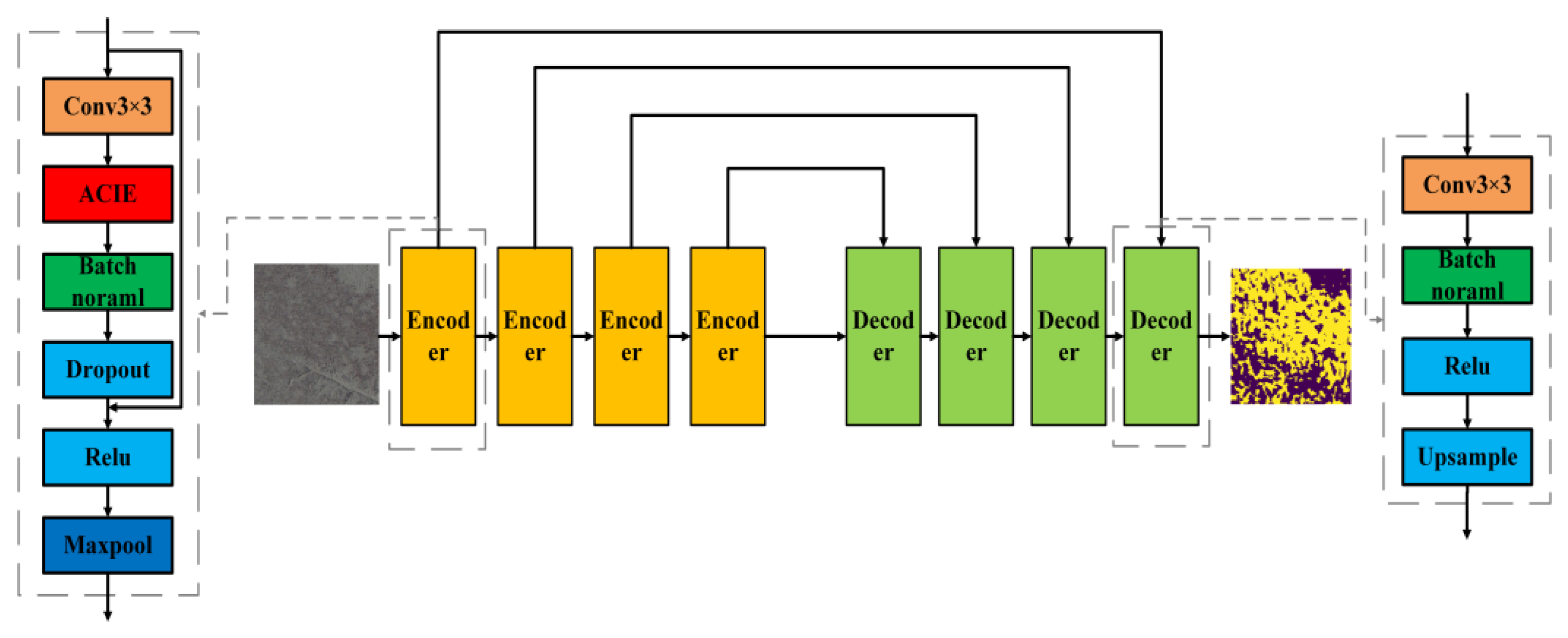
2.2.3. The ACI-Unet Model

There has been a lot of research showing that the Encoder–Decoder framework is well suited for tasks such as semantic image segmentation by gradually recovering the spatial information to capture clearer target boundaries, which is very effective in processing high-resolution imagery [35,36,37]. So, we designed an ACI-Unet based on the Unet model of the classic Encoder–Decoder framework (Figure 6). The model contains four Encoders and four decoders. The encoder is designed in the form of residual concatenation [38], which contains a downsampled 3 × 3 convolutional layer, an ACIE module, a Batch Normalization layer [39], a Dropout layer [40], a Relu layer [41], and a Maxpooling layer [42]. First after a layer of 3 × 3 convolution and then after the ACIE module for context-adaptive information extraction, and then after the BN layer and Dropout layer in order to prevent the network from the phenomenon of gradient disappearance, gradient explosion, overfitting, etc., and then residual connection of encoder’s input and Dropout’s output, residual connection can effectively ensure the depth of the model. Then it goes through the Relu layer and finally uses the maximum pooling layer to reduce the size of the feature map and then output.

Since the ACIE module consumes a lot of computational resources, in order to reduce the magnitude of the network, we preferred a simple way to design the decoder, which contains a 3 × 3 convolution, a Bath Normal layer, a Relu layer, and an Upsample layer, with the upsampling method using the nearest-neighbor upsampling and the loss function using the semantic segmentation task commonly used for the cross-entropy loss function [43].

2.3. Model Evaluation Indicators

To quantitatively evaluate the performance of the model, we evaluated the model in terms of both accuracy as well as stability. The stability of the model can be seen by the training loss during training; a more stable model should have a smooth decline in training loss during training with low oscillations.

The model accuracy evaluation uses the evaluation metrics of accuracy, recall, F1 score, and mIou [43], which are commonly used in semantic segmentation tasks, and the calculation formula is shown in

Table 1. Calculation formula for model accuracy evaluation index.

	Formula
Accuracy	$${\displaystyle \frac{TP+TN}{TP+FP+TN+FN}}$$ (9)
Recall	$${\displaystyle \frac{TP}{TP+FP}}$$ (10)
F1 score	$${\displaystyle \frac{2\times \mathrm{precision}\times \mathrm{recall}}{\mathrm{precision}+\mathrm{recall}}}$$ (11)
MIou	$$({\displaystyle \frac{TP}{TP+FP+FN}}+{\displaystyle \frac{TN}{TN+FP+FN}})/2$$ (12)

. To comprehensively evaluate the performance of our segmentation model, we report multiple commonly used metrics, including accuracy, recall, F1 score, and Mean Intersection over Union (mIou). Accuracy measures the proportion of correctly classified pixels over the total number of pixels, reflecting the overall correctness of the predictions. Recall evaluates the model’s ability to correctly identify relevant pixels, particularly focusing on how many of the actual positive pixels are retrieved, which is crucial for detecting small or sparse target regions. F1 score, as the harmonic mean of precision and recall, provides a balanced measure that accounts for both false positives and false negatives and is especially useful in imbalanced datasets. mIou is one of the most important metrics in semantic segmentation, computed as the average of Intersection over Union (IoU) across all classes. It quantifies the overlap between the predicted and ground truth regions, making it a robust indicator of segmentation quality at the class level. Together, these metrics offer a holistic view of the model’s performance from different perspectives.

TP, TN, FP, and FN can be expressed as follows:

TP: True sample size, the number of positive samples in the label and the number of positive samples in the predicted value.

TN: Number of true negative samples, number of negative samples in the label and number of negative samples in the predicted value.

FP: False Positive Sample Size, the number of negative samples in the label and the number of positive samples in the predicted value.

FN: False Negative Sample Size, number of positive samples in the label and negative samples in the predicted value.

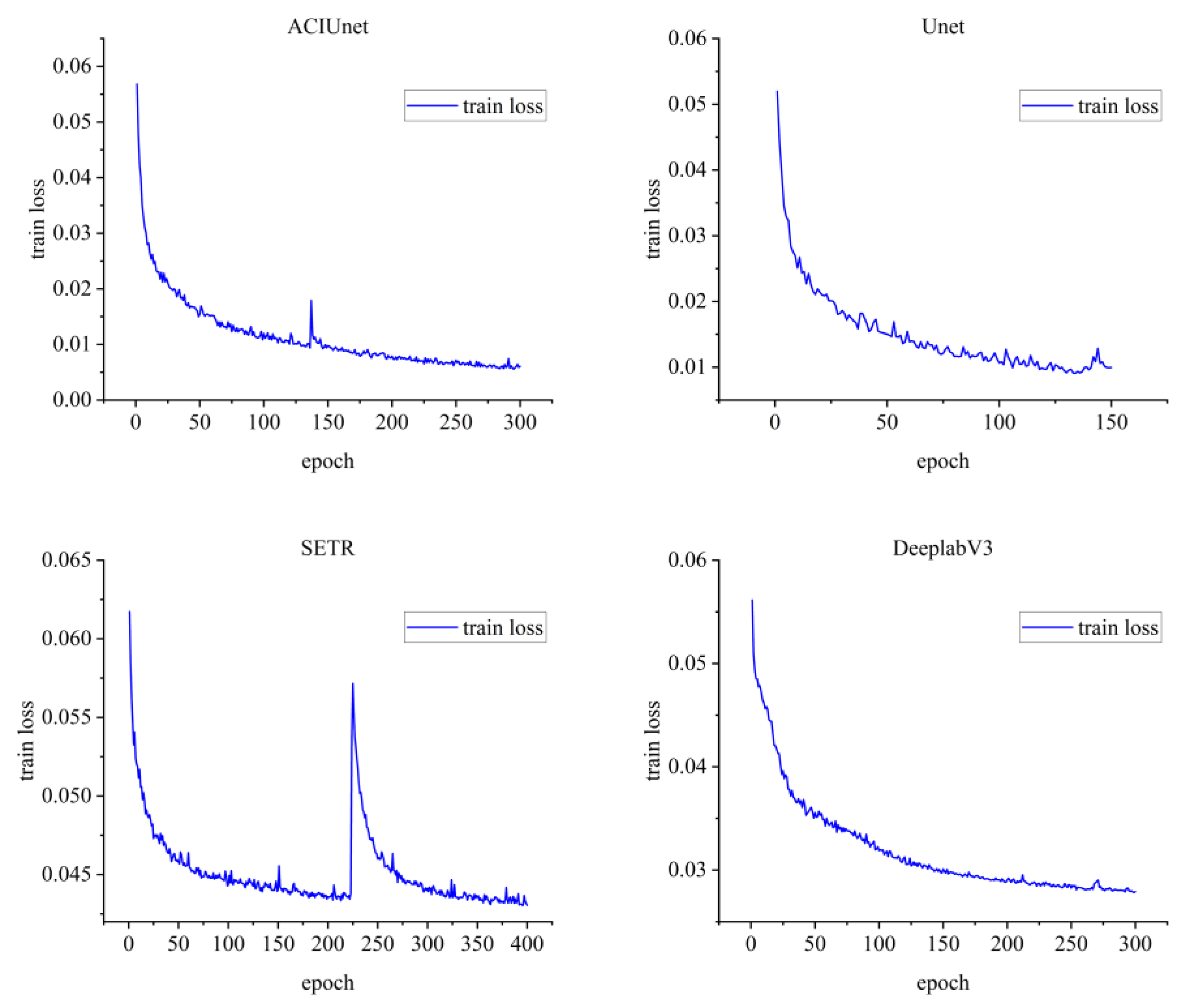
2.4. Experimental Environment and Hyperparameter Setting

We set the hyperparameters after several experiments, and the final settings are shown in

Table 2. Hyperparameter settings for each model.

	ACI-Unet	Unet	DeepLabV3	SETR
Batch_size	8	8	8	10
Lr	0.01	0.01	0.016	0.01
Dropout	0.1	0	0.1	0.1
Epochs	300	150	300	400
Optimizers	SGD	SGD	SGD	Adam
Sorters	Sigmod	Sigmod	Sigmod	softmax

. DeepLabV3 needs to set the DCNN, and the resnet34 pre-trained on Imagenet is selected. All models are trained on an NVIDIA GeForce 1070Ti, and the system is windows 10, and the programming environment is Python3.9 + pytorch1.12 + torchvision0.13.0 + cuda11.3. The loss functions were all cross-entropy. The calculation formula is shown in formula (13), where $Y$ represents the predicted value of the model, $Y’$ represents the real value of the label, and $H$ and $W$ represent the height and width of the image. In our implementation of SETR, which is a transformer-based image segmentation model, we carefully configure several key parameters to balance accuracy and computational efficiency. Specifically, we set the patch size to 32 × 32, allowing the model to process input images as non-overlapping patches for global context modeling while maintaining manageable sequence lengths. The hidden size is set to 1024, providing a rich representation capacity for each patch embedding. To reduce the spatial resolution before decoding, we apply a sampling rate of 5, which effectively downsamples the transformer output by a factor of 5. The transformer encoder is composed of 8 hidden layers and utilizes 16 attention heads per layer, enabling the model to capture multi-scale and long-range dependencies effectively. For the decoding stage, we use a feature pyramid with channel dimensions {512,256,128,64}, progressively reconstructing high-resolution segmentation maps. We adopt a naive upsampling strategy (e.g., bilinear interpolation) for its simplicity and efficiency, following the approach used in the SETR-Naive variant.

$$l_{ce}(Y,Y’)={\displaystyle \frac{{\displaystyle \sum _{i=0}^H}{\displaystyle \sum _{j=0}^W[{\displaystyle \sum _{l=1}^L{y}_{i,j}^{(l)}}\log (y{’}_{i,j}^{(l)})]}}{H\times W}}$$

(13)

3. Results

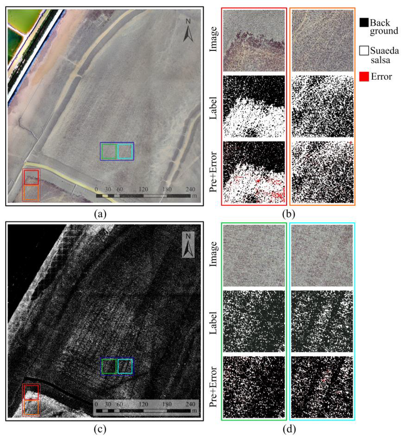
3.1. Identification Results and Analysis of Suaeda salsa

The trained ACI-Unet model was employed to predict the data from the study area constructed in Section 2.1. The binarized result of the Suaeda salsa identification is shown in Figure 7c. According to the identification results and Figure 7a, the growth area of Suaeda salsa is mainly concentrated in the shallow tidal flat areas at the junction of the sea and land. As the depth increases towards the sea, the density of the Suaeda salsa gradually decreases. This finding is consistent with the results of studies by Chen, Murray et al. [43,44]. Figure 7b shows the densely distributed and vigorously growing areas of Suaeda salsa. It can be seen that our method can identify almost all of the Suaeda salsa, but there are still some errors for particularly dense areas. Figure 7d shows the sparse distribution of Suaeda salsa, which is difficult for humans to distinguish between the target and background visually and belongs to a typical weak target. However, our method accurately identified Suaeda salsa with almost no errors, which further confirms the effectiveness of our method for weak small targets such as Suaeda salsa.

Suaeda salsa was mainly found in wetland areas demarcated by roads, and phenotypically distinct Suaeda salsa was mainly found on the side of the road close to the mudflats and on the mudflats close to the water body (Figure 7). Hydrological conditions play a crucial role in the spatial distribution of Suaeda salsa, which mainly grows in saline soils, wetlands, and coastal lands where the water level is high and the salinity is high, and the water level directly affects the plant’s root development and growth space [44]. However, for the upper-left area, which is also close to the water body, there is no Suaeda salsa growth, but green vegetation grows here. Studies have shown that as the ecosystem changes, the distribution of Suaeda salsa is also affected by other plants (e.g., herbaceous plants and shrubs), especially in areas with sufficient water, which may have an inhibitory effect on Suaeda salsa [45], which could well explain the lack of Suaeda salsa around the upper-left water body in the figure.

Suaeda salsa usually forms extensive communities in saline soils, wetlands, and coastal saline belts, and salinity is a key factor in determining whether Suaeda salsa can grow or not [46]. Suaeda salsa is capable of growing in saline environments and adapting to high-salt environments through special physiological mechanisms (e.g., salt exclusion and accumulation). Soil salinity directly affects the population growth and reproduction of Suaeda salsa; a moderate salinity helps Suaeda salsa grow, but excessive salinity limits its growth.

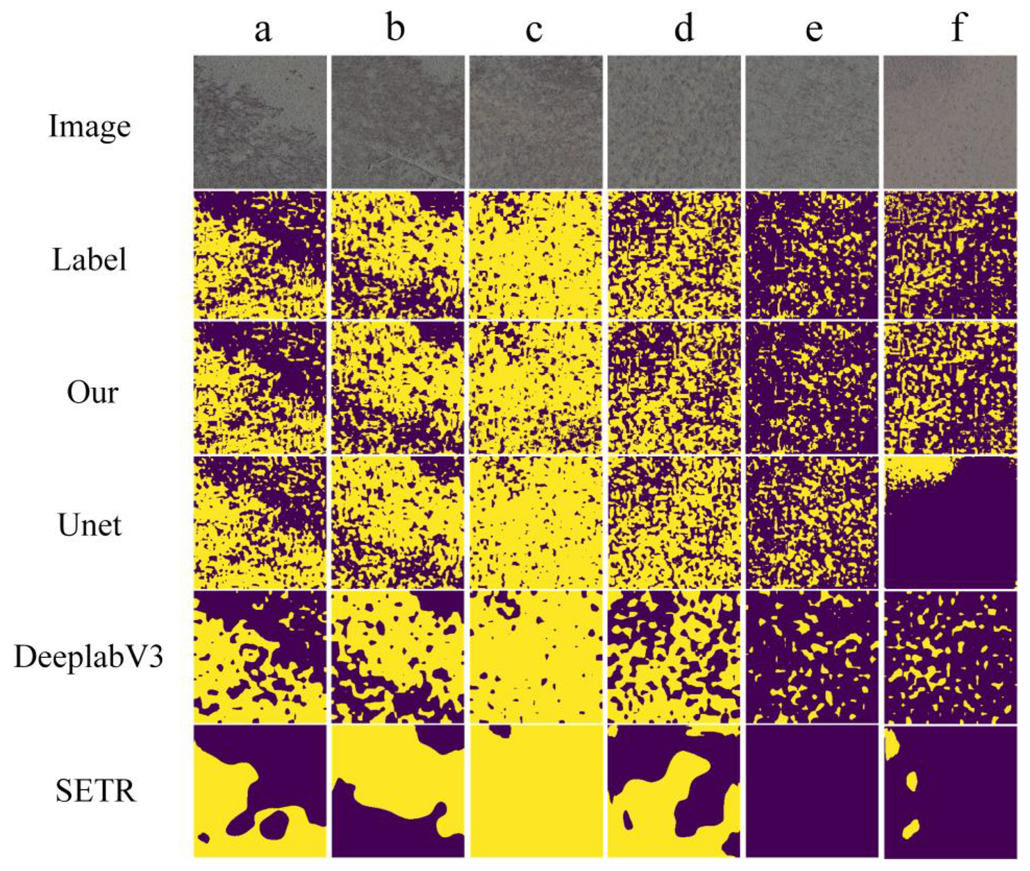
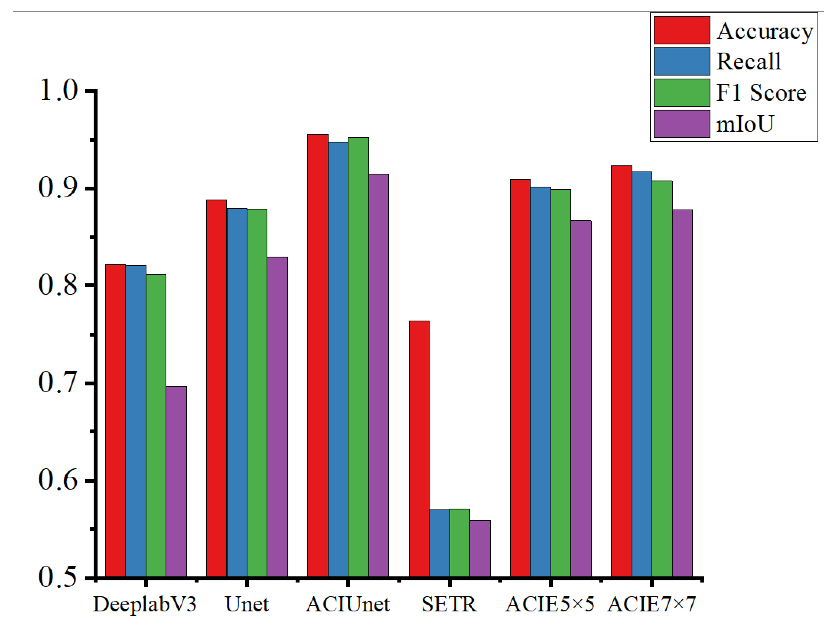
3.2. Comparison and Analysis of Model Results

In order to compare the performance of the models in this study on the UAV image Suaeda salsa extraction, three deep learning models commonly used for the semantic segmentation by Unet [24], DeepLabV3 [32], SETR [23], Linknet [47], HRnet [48], and Transunet [49] are selected for comparison. The comparative analysis is performed in terms of the result accuracy, result visualization, and training stability.

According to the model evaluation metrics in Section 2.3, the performance of the metrics computed for all models on the test set is shown in

Table 3. Results of prediction accuracy indicators for each model.

	Accuracy (%)	Recall (%)	F1 Score (%)	MIou (%)
ACI-Unet	95.55	94.73	95.21	91.44
Unet	88.79	87.93	87.84	82.95
DeepLabV3	82.15	82.07	81.10	69.69
SETR	76.33	56.96	57.07	55.92
Linknet	81.96	62.36	52.93	41.30
HRnet	91.29	73.15	66.36	58.18
Transunet	92.77	71.76	72.42	67.40

. According to Table 3, it can be seen that this paper’s method is the highest among all the evaluation metrics. Compared with DeepLabV3, SETR, and Unet, our model has a large improvement in all the indicators, and all four indicators are above 90%, among which the mIou has the most obvious improvement, which is 8.49% compared with Unet, 21.75% compared with DeepLabV3, and 35.52% compared with SETR. This indicates that our model is more accurate in boundary and area predictions. In terms of accuracy, this paper’s model improves by 6.76%, 13.4%, and 19.22% compared to Unet, DeepLabV3, and SETR, respectively. In terms of recall, this paper’s model improves by 6.8%, 12.66%, and 37.77% compared to Unet, DeepLabV3, and SETR, respectively. In addition, the Unet model also has a notable accuracy, which indicates that the use of jump connection joint context features is an effective way to extract Suaeda salsa. The accuracy of the SETR model is only 76.33% compared to other CNN models, and the other three metrics are very poor, with less than 60% for all three metrics. In addition, the performance of HRnet and Transunet in terms of accuracy is also satisfactory, but other indicators still have a certain gap compared with our method, which proves that our model has a good recognition effect for both positive and negative samples.

Six images representative of different phenotypes of Suaeda salsa were selected in the test set, and the model predictions were visualized as shown in Figure 8. Here we show the visualization results of Unet, DeepLabV3, and SETR, which are commonly used in the field of remote sensing segmentation. According to Figure 8a–d, it can be seen that for regions with dense Suaeda salsa, both Unet and ACI-Unet can achieve good prediction results. However, for the region of weak Suaeda salsa, as shown in Figure 8e,f, the prediction results of models other than this study are not very satisfactory, and our method can accurately segment the details of the spatial distribution of Suaeda salsa. DeepLabV3 lacks sufficient spatial information to represent the gaps between Suaeda salsa, which may be due to the fact that the design of the null convolution exaggerates the sensory field while omitting certain spatial detail information [50]. Unet does not effectively recognize images where the Suaeda salsa is not clearly represented, and there are large areas of misrecognition. SETR is the worst, only recognizing a general distribution in areas where Suaeda salsa targets are obvious.

The results of all model training are shown in Figure 9. In terms of model accuracy, ACI-Unet performs the best, and the training loss of our method converges at around 0.006, Unet converges at around 0.01, SETR converges at around 0.42, and DeepLabV3 converges at around 0.28. In terms of training efficiency, according to the training loss curve, it can be seen that Unet converges the fastest, which is probably due to the small number of Unet model parameters, followed by ACI-Unet, and DeepLabV3 has the worst training efficiency. In terms of model stability, DeepLabV3 performs the best, followed by ACI-Unet, and SETR has the worst stability.

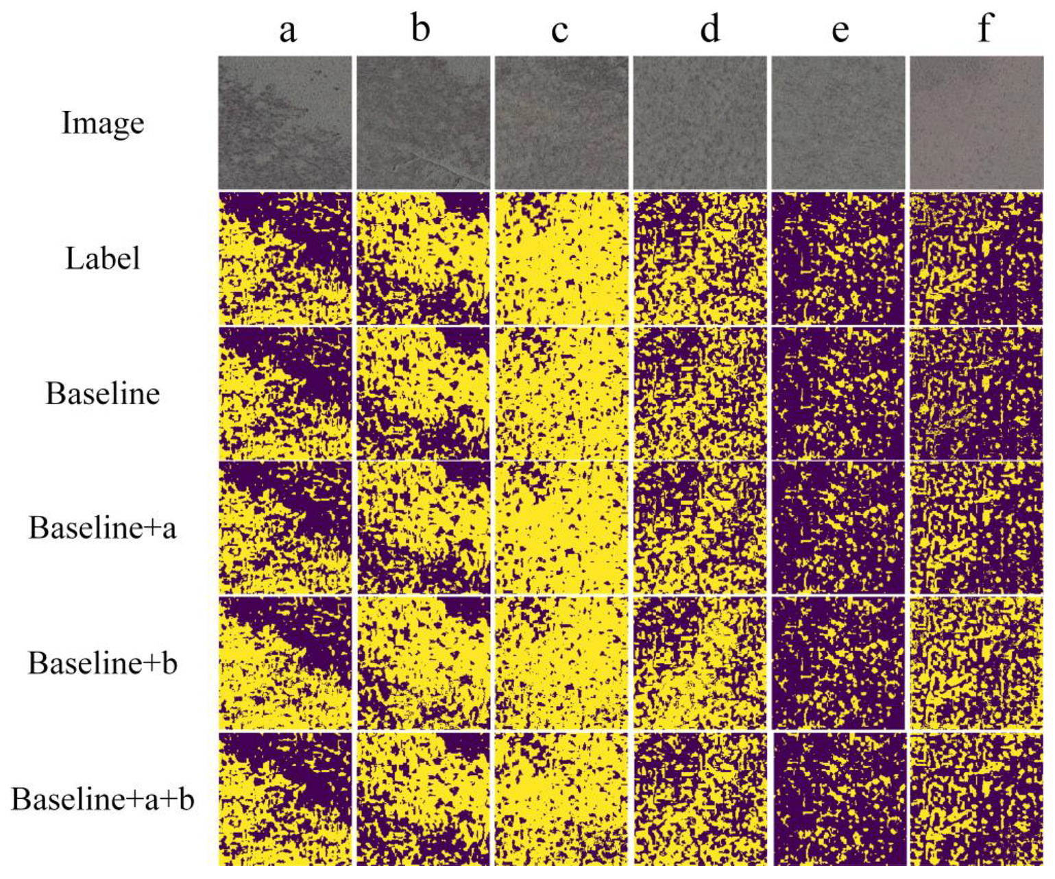
3.3. Result of Ablation Experiments

In order to verify the enhancement effect of the spatial and feature selection modules on ACIE, the ablation experiment of the model is designed in this section. The baseline network is regarded as the baseline, the spatial selection module is named as a, and the feature selection module is named as b. The baseline + a, baseline + b, and baseline + a + b (ACI-Unet) are conducted, and the calculation results of the accuracy indexes on the test set are shown in

Table 4. Results of ablation experiment accuracy index.

	Accuracy (%)	Recall (%)	F1 Score (%)	MIou (%)
Baseline	93.26	89.33	89.01	87.06
Baseline + a	94.70	90.38	90.39	88.54
Baseline + b	94.50	90.44	90.47	87.57
Baseline + a + b	95.55	94.73	95.21	91.44

, and the prediction results are visualized as shown in Figure 10. It can be seen that each module has been enhanced to a certain extent, which further proves the rationality of our design of the ACIE module.

4. Discussion

4.1. The Evaluation of the ACI-Unet MODEL Based on Ablation Experiments

When extracting Suaeda salsa from remote sensing images, it often faces the challenge of a small target scale and scattered distribution. Suaeda salsa vegetation often presents as small patches with uneven distributions, which makes it easy for conventional convolution to ignore its contextual information. Therefore, we designed an ACIE module to enhance the contextual understanding ability of the feature representation while preserving spatial details, improving the recognition performance of small targets such as Suaeda salsa. Traditional context modeling methods, such as dilated convolution and pyramid pooling, often introduce downsampling or sparse sampling, which may cause information damage to small targets. This module maintains a consistent input–output resolution throughout the entire operation to preserve spatial details to the greatest extent possible. So, we designed the ACIE module based on large kernel convolution, which can adaptively capture contextual information. According to the calculation results, the ACIE, spatial selection module, and feature selection module all have some improvement on the model effect compared with the baseline. In accuracy, ACIE can improve by 2.29%, the spatial selection module can improve by 1.44%, and the feature selection module can improve by 1.24%. In terms of recall, ACIE improves by 5.4%, the spatial selection module improves by 1.08%, and the feature selection module improves by 1.11%. For the F1 score, ACIE improved by 6.2%, the spatial selection module by 1.38%, and the feature selection module by 1.46%. In terms of the mIou, ACIE improved by 4.38%, the spatial selection module by 1.48%, and the feature selection module by 0.51%. The prediction results are visualized as shown in Figure 10. It can be seen that, in addition to the mIou, the feature selection module and the spatial selection module have comparable improvement effects, and the spatial selection module has a better improvement effect in the mIou. In simple terms, the mIou is the average of the overlapping region between the predicted segmentation and label divided by the joint region between the predicted segmentation and label, so the mIou takes into account more spatial region prediction effects [51]. It is worth mentioning that the baseline constructed in this paper is higher compared to all the accuracy metrics of the comparison models selected in Section 3, which indicates that the baseline constructed in this paper is more accurate and effective in accomplishing the task of this paper.

4.2. The Analysis of the Causes of Different Identification Results

This section discusses the effect of the Suaeda salsa recognition with different contextual information. The different models used in this study extract contextual information in different ways. SETR uses a transform-encoder based on the self-attention mechanism, which extracts global contextual information [52], while Unet, DeepLabV3, and ACI-Unet use a convolutional-layer-based encoder, which extracts local contextual information [31]. Using the metrics proposed in Section 2.3 to represent the recognition effect of Suaeda salsa, in addition, we also include the results of different convolutional kernel sizes (5 × 5 and 5 × 5, 7 × 7 and 7 × 7) of the ACIE module to explore the local context information of Suaeda salsa at different scales and the reasonableness of our design of the ACIE module, and the results are shown in Figure 11. Based on the results of the recognition accuracy of the different models, it can be seen that for the task of Suaeda salsa recognition, the modeling of the local contextual information is better than that of the global contextual information. Sainath, T. N. et al. [53] found that the local receptive field of the volume and neural network is better for the recognition of small targets and targets with large phenotypic differences, and, as mentioned before, because of the influence of topography, salinity, etc., Suaeda salsa shows different phenotypes under different growth conditions [9], with inconsistent sizes, irregular shapes, and inconsistent colors, which coincides with the findings of Sainath, T. N. This can explain why CNNs, which are more adequate to capture local contextual information, exhibit better performances.

Different CNN models extract different local contextual information. In layman’s terms, CNNs are better able to capture local textures, edges, and small-scale target features through the design of local sensory fields. Especially when dealing with complex, multi-phenotype targets, local contextual information helps to extract details related to the target morphology. Unet uses 3 × 3 convolutional kernels to extract contextual information, and such an approach focuses more on detail information. The ACI-Unet we used relies on increasing the size of the convolutional kernel and attention mechanism to realize the adaptive extraction of multi-scale contextual information. DeepLabv3 realizes the extraction of richer contextual information by expanding the local receptive field through cavity convolution. According to Figure 11, it can be seen that Unet and ACI-Unet possess a more effective recognition effect compared to DeepLabv3, which indicates that the information of spatial details can better help the model to recognize the Suaeda salsa, such as the color, texture, edge, and other information. However, the ACI-Unet with the addition of the ACIE module has another good improvement compared to Unet, which indicates that the expansion of the local receptive field can better access the contextual information of Suaeda salsa. However, unlike DeepLabv3, we use large kernel convolution instead of null convolution. For the choice of different convolution kernel sizes, we give the results of the Suaeda salsa recognition accuracy using dual 5 × 5 and dual 7 × 7 sizes, and finally we choose the combination of 5 × 5 and 7 × 7 convolution kernel sizes.

5. Conclusions

In this study, we designed a network ACI-Unet that can adaptively extract contextual information to achieve a high-precision UAV image recognition of Suaeda salsa in response to the difficulty of recognizing Suaeda salsa targets that are weak, small, and different sizes and morphologies with irregular shapes and inconsistent colors. The main research results and conclusions obtained are as follows:

(1)

An adaptive contextual information extraction module based on a large kernel convolution and attention mechanism is designed, which can be embedded into any kind of network as a multi-scale feature extractor without changing the resolution and can help the model to better extract the contextual adaptive information.

(2)

The ACI-Unet model constructed in this paper can realize a high-precision Suaeda salsa recognition for UAV imagery. For Suaeda salsa diversity, our method has a good recognition effect both for Suaeda salsa with a large shape, obvious color, and dense growth area and for Suaeda salsa with a small shape, less obvious color, and sparse growth area. In terms of precision, all four metrics were above 90%.

(3)

Our model compares the results of the Suaeda salsa extraction with existing models commonly used for semantic segmentation and finds that they are all improved, especially for the weak Suaeda salsa targets with inconspicuous features, which can accurately segment the spatial distribution details of Suaeda salsa.

There are still some shortcomings in this study. Firstly, in the selection of data, the use of visible images has some limitations in their spectral resolution. Secondly, in terms of modeling, the modeling approach based on the deep learning method is poorly interpretable and cannot analyze the corresponding feature information of Suaeda salsa. Future studies should consider incorporating more spectral information to analyze the properties of Suaeda salsa.

References

1. Gao, F.; Wu, L.; Jia, S.; Sun, Q.; Liu, G. Study on evaluation and impact mechanism of beach lowering restoration effect of Suaeda Heteroptera wetland in Liaohe estuary. Environ. Ecol. 2022, 4, 49–53. [Google Scholar]
2. Yang, C.; Wang, L.; Su, F.; Li, H. Characteristics of soil salinity in the distribution area of Suaedaheteroptera in Liaohe estuary wetlands. Sci. Soil Water Conserv. 2019, 17, 117–123. [Google Scholar]
3. Li, Y.; Wang, Z.; Zhao, C.; Jia, M.; Ren, C.; Mao, D.; Yu, H. Research on spatial-temporal dynamics of Suaeda salsa in Liaohe estuary and its identification mechanism using remote sensing. Remote Sens. Nat. Resour. 2024, 195–203. [Google Scholar]
4. Zhang, N.; Mao, D.; Feng, K.; Zhen, J.; Xiang, H.; Ren, Y. Classification of wetland plant communities in the Yellow River Delta based on GEE and multi-source remote sensing data. Remote Sens. Nat. Resour. 2024, 265–273. [Google Scholar]
5. Ke, Y.; Han, Y.; Cui, L.; Sun, P.; Min, Y.; Wang, Z.; Zhuo, Z.; Zhou, Q.; Yin, X.; Zhou, D. Suaeda salsa Spectral Index for Suaeda salsa Mapping and Fractional Cover Estimation in Intertidal Wetlands. ISPRS J. Photogramm. Remote Sens. 2024, 207, 104–121. [Google Scholar] [CrossRef]
6. Gao, T. Research on Community Information Extraction of Suaeda salsa Based on UAV Multispectral Data. Master’s Thesis, Dalian Ocean University, Dalian, China, June 2024. [Google Scholar] [CrossRef]
7. Ren, G.; Zhang, J.; Wang, W.; Geng, Y.; Chen, Y.; Ma, Y. Reeds and suaeda biomass estimation model based on HJ-1 hyper-spectal image in the Yellow River Estuary. J. Mar. Sci. 2014, 32, 27–34. [Google Scholar]
8. Du, Y.; Wang, J.; Liu, Z.; Yu, H.; Li, Z.; Cheng, H. Evaluation on Spaceborne Multispectral Images, Airborne Hyperspectral, and LiDAR Data for Extracting Spatial Distribution and Estimating Aboveground Biomass of Wetland Vegetation Suaeda salsa. IEEE J. Sel. Top. Appl. Earth Obs. Remote Sens. 2019, 12, 200–209. [Google Scholar] [CrossRef]
9. Zhang, S.; Tian, Q.; Lu, X.; Li, S.; He, S.; Zhang, X.; Liu, K. Enhancing Chlorophyll Content Monitoring in Coastal Wetlands: Sentinel-2 and Soil-Removed Semi-Empirical Models for Phenotypically Diverse Suaeda salsa. Ecol. Indic. 2024, 167, 112686. [Google Scholar] [CrossRef]
10. Zhang, S.; Tian, J.; Lu, X.; Tian, Q.; He, S.; Lin, Y.; Li, S.; Zheng, W.; Wen, T.; Mu, X.; et al. Monitoring of Chlorophyll Content in Local Saltwort Species Suaeda salsa under Water and Salt Stress Based on the PROSAIL-D Model in Coastal Wetland. Remote Sens. Environ. 2024, 306, 114117. [Google Scholar] [CrossRef]
11. Maggiori, E.; Tarabalka, Y.; Charpiat, G.; Alliez, P. Convolutional Neural Networks for Large-Scale Remote-Sensing Image Classification. IEEE Trans. Geosci. Remote Sens. 2017, 55, 645–657. [Google Scholar] [CrossRef]
12. Lv, X.; Ming, D.; Chen, Y.; Wang, M. Very High Resolution Remote Sensing Image Classification with SEEDS-CNN and Scale Effect Analysis for Superpixel CNN Classification. Int. J. Remote Sens. 2019, 40, 506–531. [Google Scholar] [CrossRef]
13. Zhang, C.; Wei, S.; Ji, S.; Lu, M. Detecting Large-Scale Urban Land Cover Changes from Very High Resolution Remote Sensing Images Using CNN-Based Classification. ISPRS Int. J. Geo-Inf. 2019, 8, 189. [Google Scholar] [CrossRef]
14. Li, Z.; Shen, H.; Cheng, Q.; Liu, Y.; You, S.; He, Z. Deep Learning Based Cloud Detection for Medium and High Resolution Remote Sensing Images of Different Sensors. ISPRS J. Photogramm. Remote Sens. 2019, 150, 197–212. [Google Scholar] [CrossRef]
15. Hu, K.; Zhang, E.; Xia, M.; Weng, L.; Lin, H. MCANet: A Multi-Branch Network for Cloud/Snow Segmentation in High-Resolution Remote Sensing Images. Remote Sens. 2023, 15, 1055. [Google Scholar] [CrossRef]
16. Fu, H.; Fu, B.; Shi, P. An Improved Segmentation Method for Automatic Mapping of Cone Karst from Remote Sensing Data Based on DeepLab V3+ Model. Remote Sens. 2021, 13, 441. [Google Scholar] [CrossRef]
17. Kleinschroth, F.; Banda, K.; Zimba, H.; Dondeyne, S.; Nyambe, I.; Spratley, S.; Winton, R.S. Drone Imagery to Create a Common Understanding of Landscapes. Landsc. Urban Plan. 2022, 228, 104571. [Google Scholar] [CrossRef]
18. Huang, Y.; Chen, J.; Huang, D. UFPMP-Det:Toward Accurate and Efficient Object Detection on Drone Imagery. Proc. AAAI Conf. Artif. Intell. 2022, 36, 1026–1033. [Google Scholar] [CrossRef]
19. Jintasuttisak, T.; Edirisinghe, E.; Elbattay, A. Deep Neural Network Based Date Palm Tree Detection in Drone Imagery. Comput. Electron. Agric. 2022, 192, 106560. [Google Scholar] [CrossRef]
20. Du, D.; Zhu, P.; Wen, L.; Bian, X.; Lin, H.; Hu, Q.; Peng, T.; Zheng, J.; Wang, X.; Zhang, Y.; et al. VisDrone-DET2019: The Vision Meets Drone Object Detection in Image Challenge Results. In Proceedings of the IEEE/CVF International Conference on Computer Vision (ICCV) Workshops, Seoul, Republic of Korea, 27 October–2 November 2019. [Google Scholar]
21. Garcia-Garcia, A.; Orts-Escolano, S.; Oprea, S.; Villena-Martinez, V.; Garcia-Rodriguez, J. A Review on Deep Learning Techniques Applied to Semantic Segmentation. arXiv 2017. [Google Scholar] [CrossRef]
22. Liu, J.; Wang, Z.; Cheng, K. An Improved Algorithm for Semantic Segmentation of Remote Sensing Images Based on DeepLabv3+. In Proceedings of the 5th International Conference on Communication and Information Processing, Chongqing, China, 15–17 November 2019; ACM: Chongqing China, 2019; pp. 124–128. [Google Scholar]
23. Zheng, S.; Lu, J.; Zhao, H.; Zhu, X.; Luo, Z.; Wang, Y.; Fu, Y.; Feng, J.; Xiang, T.; Torr, P.H.S.; et al. Rethinking Semantic Segmentation From a Sequence-to-Sequence Perspective With Transformers. In Proceedings of the IEEE/CVF Conference on Computer Vision and Pattern Recognition (CVPR), Nashville, TN, USA, 20–25 June 2021; pp. 6881–6890. [Google Scholar]
24. Ronneberger, O.; Fischer, P.; Brox, T. U-Net: Convolutional Networks for Biomedical Image Segmentation. arXiv 2015. [Google Scholar] [CrossRef]
25. Minaee, S.; Boykov, Y.Y.; Porikli, F.; Plaza, A.J.; Kehtarnavaz, N.; Terzopoulos, D. Image Segmentation Using Deep Learning: A Survey. IEEE Trans. Pattern Anal. Mach. Intell. 2022, 44, 3523–3542. [Google Scholar] [CrossRef] [PubMed]
26. Wang, H.; Huang, Z.; Ye, J.; Tu, C.; Yang, Y.; Du, S.; Deng, Z.; Ma, C.; Niu, J.; He, J. An Evaluation of U-Net in Renal Structure Segmentation. arXiv 2022. [Google Scholar] [CrossRef]
27. Zunair, H.; Ben Hamza, A. Sharp U-Net: Depthwise Convolutional Network for Biomedical Image Segmentation. Comput. Biol. Med. 2021, 136, 104699. [Google Scholar] [CrossRef] [PubMed]
28. Shamsolmoali, P.; Zareapoor, M.; Wang, R.; Zhou, H.; Yang, J. A Novel Deep Structure U-Net for Sea-Land Segmentation in Remote Sensing Images. IEEE J. Sel. Top. Appl. Earth Obs. Remote Sens. 2019, 12, 3219–3232. [Google Scholar] [CrossRef]
29. Guo, M.-H.; Xu, T.-X.; Liu, J.-J.; Liu, Z.-N.; Jiang, P.-T.; Mu, T.-J.; Zhang, S.-H.; Martin, R.R.; Cheng, M.-M.; Hu, S.-M. Attention Mechanisms in Computer Vision: A Survey. Comput. Vis. Media 2022, 8, 331–368. [Google Scholar] [CrossRef]
30. Fu, J.; Liu, J.; Tian, H.; Li, Y.; Bao, Y.; Fang, Z.; Lu, H. Dual Attention Network for Scene Segmentation. In Proceedings of the IEEE/CVF Conference on Computer Vision and Pattern Recognition (CVPR), Long Beach, CA, USA, 15–20 June 2019. [Google Scholar]
31. Li, Z.; Liu, F.; Yang, W.; Peng, S.; Zhou, J. A Survey of Convolutional Neural Networks: Analysis, Applications, and Prospects. IEEE Trans. Neural Netw. Learn. Syst. 2022, 33, 6999–7019. [Google Scholar] [CrossRef]
32. Lin, T.-Y.; Dollár, P.; Girshick, R.; He, K.; Hariharan, B.; Belongie, S. Feature Pyramid Networks for Object Detection. arXiv 2016. [Google Scholar] [CrossRef]
33. Woo, S.; Park, J.; Lee, J.-Y.; Kweon, I.S. CBAM: Convolutional Block Attention Module. arXiv 2018. [Google Scholar] [CrossRef]
34. Hu, J.; Shen, L.; Sun, G. Squeeze-and-Excitation Networks. In Proceedings of the IEEE Conference on Computer Vision and Pattern Recognition (CVPR), Salt Lake City, UT, USA, 18–23 June 2018. [Google Scholar]
35. Chen, L.-C.; Zhu, Y.; Papandreou, G.; Schroff, F.; Adam, H. Encoder-Decoder with Atrous Separable Convolution for Semantic Image Segmentation. In Proceedings of the European Conference on Computer Vision (ECCV), Munich, Germany, 8–14 September 2018. [Google Scholar]
36. Tian, Z.; He, T.; Shen, C.; Yan, Y. Decoders Matter for Semantic Segmentation: Data-Dependent Decoding Enables Flexible Feature Aggregation. In Proceedings of the IEEE/CVF Conference on Computer Vision and Pattern Recognition (CVPR), Long Beach, CA, USA, 15–20 June 2019. [Google Scholar]
37. Wang, S.; Hou, X.; Zhao, X. Automatic Building Extraction From High-Resolution Aerial Imagery via Fully Convolutional Encoder-Decoder Network With Non-Local Block. IEEE Access 2020, 8, 7313–7322. [Google Scholar] [CrossRef]
38. He, K.; Zhang, X.; Ren, S.; Sun, J. Deep Residual Learning for Image Recognition. In Proceedings of the 2016 IEEE Conference on Computer Vision and Pattern Recognition (CVPR), Las Vegas, NV, USA, 27–30 June 2016; IEEE: Las Vegas, NV, USA, 2016; pp. 770–778. [Google Scholar]
39. Ioffe, S.; Szegedy, C. Batch Normalization: Accelerating Deep Network Training by Reducing Internal Covariate Shift. In Proceedings of the 32nd International Conference on Machine Learning, Lille, France, 6–11 July 2015; Bach, F., Blei, D., Eds.; PMLR: Lille, France, 2015; Volume 37, pp. 448–456. [Google Scholar]
40. Srivastava, N.; Hinton, G.; Krizhevsky, A.; Sutskever, I.; Salakhutdinov, R. Dropout: A Simple Way to Prevent Neural Networks from Overfitting. J. Mach. Learn. Res. 2014, 15, 1929–1958. [Google Scholar]
41. Glorot, X.; Bordes, A.; Bengio, Y. Deep Sparse Rectifier Neural Networks. In Proceedings of the Fourteenth International Conference on Artificial Intelligence and Statistics, Fort Lauderdale, FL, USA, 11–13 April 2011; Gordon, G., Dunson, D., Dudík, M., Eds.; PMLR: Fort Lauderdale, FL, USA, 2011; Volume 15, pp. 315–323. [Google Scholar]
42. Lecun, Y.; Bottou, L.; Bengio, Y.; Haffner, P. Gradient-Based Learning Applied to Document Recognition. Proc. IEEE 1998, 86, 2278–2324. [Google Scholar] [CrossRef]
43. Goodfellow, I.; Bengio, Y.; Courville, A. Deep Learning; MIT Press: Cambridge, MA, USA, 2016; ISBN 978-0-262-33737-3. [Google Scholar]
44. Short, F.T.; Kosten, S.; Morgan, P.A.; Malone, S.; Moore, G.E. Impacts of Climate Change on Submerged and Emergent Wetland Plants. Aquat. Bot. 2016, 135, 3–17. [Google Scholar] [CrossRef]
45. Chong, K.Y.; Raphael, M.B.; Carrasco, L.R.; Yee, A.T.K.; Giam, X.; Yap, V.B.; Tan, H.T.W. Reconstructing the Invasion History of a Spreading, Non-Native, Tropical Tree through a Snapshot of Current Distribution, Sizes, and Growth Rates. Plant Ecol. 2017, 218, 673–685. [Google Scholar] [CrossRef]
46. Jolly, I.D.; McEwan, K.L.; Holland, K.L. A Review of Groundwater–Surface Water Interactions in Arid/Semi-arid Wetlands and the Consequences of Salinity for Wetland Ecology. Ecohydrology 2008, 1, 43–58. [Google Scholar] [CrossRef]
47. Chaurasia, A.; Culurciello, E. LinkNet: Exploiting Encoder Representations for Efficient Semantic Segmentation. In Proceedings of the 2017 IEEE Visual Communications and Image Processing (VCIP), St. Petersburg, FL USA, 10–13 December 2017; IEEE: St. Petersburg, FL, USA, 2017; pp. 1–4. [Google Scholar]
48. Sun, K.; Xiao, B.; Liu, D.; Wang, J. Deep High-Resolution Representation Learning for Human Pose Estimation. In Proceedings of the IEEE/CVF Conference on Computer Vision and Pattern Recognition (CVPR), Long Beach, CA, USA, 15–20 June 2019. [Google Scholar]
49. Chen, J.; Lu, Y.; Yu, Q.; Luo, X.; Adeli, E.; Wang, Y.; Lu, L.; Yuille, A.L.; Zhou, Y. TransUNet: Transformers Make Strong Encoders for Medical Image Segmentation. arXiv 2021. [Google Scholar] [CrossRef]
50. Chen, L.-C.; Papandreou, G.; Schroff, F.; Adam, H. Rethinking Atrous Convolution for Semantic Image Segmentation. arXiv 2017. [Google Scholar] [CrossRef]
51. Zhang, H.; Dana, K.; Shi, J.; Zhang, Z.; Wang, X.; Tyagi, A.; Agrawal, A. Context Encoding for Semantic Segmentation. In Proceedings of the IEEE Conference on Computer Vision and Pattern Recognition (CVPR), Salt Lake City, UT, USA, 18–23 June 2018. [Google Scholar]
52. Han, K.; Wang, Y.; Chen, H.; Chen, X.; Guo, J.; Liu, Z.; Tang, Y.; Xiao, A.; Xu, C.; Xu, Y.; et al. A Survey on Vision Transformer. IEEE Trans. Pattern Anal. Mach. Intell. 2023, 45, 87–110. [Google Scholar] [CrossRef]
53. Bruna, J.; Sprechmann, P.; LeCun, Y. Source Separation with Scattering Non-Negative Matrix Factorization. In Proceedings of the 2015 IEEE International Conference on Acoustics, Speech and Signal Processing (ICASSP), Brisbane, QLD, Australia, 19–24 April 2015; IEEE: South Brisbane, QLD, Australia, 2015; pp. 1876–1880. [Google Scholar]
Figure 1. The schematic diagram of Suaeda salsa, the subject of this study.
Remotesensing 17 02022 g001
Figure 2. A schematic diagram of the study area.
Remotesensing 17 02022 g002
Figure 3. A partial presentation of the model training dataset.
Remotesensing 17 02022 g003
Figure 4. The schematic diagram of the Unet model [24].
Remotesensing 17 02022 g004
Figure 5. Schematic diagram of ACIE module.
Remotesensing 17 02022 g005
Figure 6. ACI-Unet model diagram.
Remotesensing 17 02022 g006
Figure 7. Results of the binarization of Suaeda salsa identification in the study area. (a) Test images of the research area, (b) Enlarge the result within the red orange box, (c) Binary extraction results of test image Suaeda salsa, (d) Enlarge the result within the green and blue boxes.
Remotesensing 17 02022 g007
Figure 8. Visualization of model prediction results. (ad) Dense distribution of Suaeda salsa, (e,f) Sparse distribution of Suaeda salsa.
Remotesensing 17 02022 g008
Figure 9. Training loss curve.
Remotesensing 17 02022 g009
Figure 10. Visualization of ablation experiment results. (ad) Dense distribution of Suaeda salsa (e,f) Sparse distribution of Suaeda salsa.
Remotesensing 17 02022 g010
Figure 11. Recognition results of Suaeda salsa with different contextual information.
Remotesensing 17 02022 g011