Next Article in Journal
Effects of Drought Stress on the Relationship Between Solar-Induced Chlorophyll Fluorescence and Gross Primary Productivity in a Chinese Cork Oak Plantation
Previous Article in Journal
Lightweight Infrared Small Target Detection Method Based on Linear Transformer
Previous Article in Special Issue
Subsurface Cavity Imaging Based on UNET and Cross–Hole Radar Travel–Time Fingerprint Construction
 
 
Due to scheduled maintenance work on our database systems, there may be short service disruptions on this website between 10:00 and 11:00 CEST on June 14th.
Article

Mapping Mountain Permafrost via GPR-Augmented Machine Learning in the Northeastern Qinghai–Tibet Plateau

1
Cryosphere Research Station on the Qinghai-Tibet Plateau, State Key Laboratory of Cryospheric Science and Frozen Soil Engineering, Northwest Institute of Eco-Environment and Resources, Chinese Academy of Sciences, Lanzhou 730030, China
2
Northwest Institute of Eco-Environment and Resources, Chinese Academy of Sciences, Lanzhou 730030, China
3
National Cryosphere Desert Data Center, Lanzhou 730030, China
4
School of Geographical Sciences, Nanjing University of Information Science & Technology (NUIST), Nanjing 210044, China
*
Author to whom correspondence should be addressed.
Remote Sens. 2025, 17(12), 2015; https://doi.org/10.3390/rs17122015
Submission received: 13 May 2025 / Revised: 6 June 2025 / Accepted: 9 June 2025 / Published: 11 June 2025
(This article belongs to the Special Issue Advanced Ground-Penetrating Radar (GPR) Technologies and Applications)

Abstract

:
Accurate permafrost mapping in mountainous regions is hindered by sparse in situ observations and heterogeneous terrain. This study develops a GPR-augmented machine learning framework to map mountain permafrost in the northeastern Qinghai–Tibet Plateau. A total of 1037 presence–absence samples were compiled from boreholes, soil pits, 128 GPR transects collected in 2009, and 22 additional empirical points above 4700 m, covering diverse topographic and thermal conditions. Thirteen classification algorithms were evaluated using 5-fold cross-validation repeated 40 times, with LightGBM, CatBoost, XGBoost, and RF achieving top performance (F1 > 0.98). Elevation-based spatial comparisons revealed that LightGBM and CatBoost produced more terrain-adaptive predictions at high altitudes and slope transitions. Aspect-controlled permafrost boundaries were captured, with modeled lower elevation limits varying by >200 m across slope directions. SHAP analysis showed that climate and soil variables contributed nearly 80% to model outputs, with LST, FDD, BD, and TDD being dominant. Several predictors exhibited threshold or nonlinear responses, reinforcing their physical relevance. Additional experiments confirmed that integration of GPR and high-elevation constraint samples significantly improved model generalization, especially in underrepresented terrain zones. This study demonstrates that a GPR-augmented machine learning framework can support cost-effective, physically informed mapping of frozen ground in complex alpine environments.

1. Introduction

Permafrost, defined as ground that remains at or below 0 °C for at least two consecutive years, plays a critical role in regional hydrology, carbon cycling, and infrastructure stability across high-latitude and high-altitude environments such as the Qinghai–Tibet Plateau (QTP), the Arctic, and sub-Arctic mountains [1,2,3]. With climate warming accelerating, permafrost degradation has emerged as a major concern due to its potential to amplify greenhouse gas emissions and disrupt surface stability [4,5,6,7]. Accurate mapping of permafrost extent is therefore essential for understanding environmental risk, managing hydrological systems, and guiding infrastructure design in cryospheric regions [8,9,10,11].
Traditional modeling approaches, including physics-based energy balance models [12,13,14] and empirical–statistical models [15,16,17], have provided foundational insights into permafrost dynamics. However, these methods are often constrained by high data requirements, strong assumptions, and limited capacity to model complex nonlinear interactions [16,18]. Machine learning (ML) models offer a promising alternative, capable of capturing nonlinear interactions across diverse environmental predictors [19,20]. Successful applications of ML for permafrost mapping have been demonstrated across Arctic and mountainous regions, including the Carpathians, northeastern China, and the Tibetan Plateau [21,22,23,24,25].
Nevertheless, ML-based permafrost studies face persistent challenges; observation data are typically sparse and spatially biased, especially in rugged alpine terrain, and model outputs often lack interpretability in terms of underlying physical mechanisms. Ground-penetrating radar (GPR) provides a cost-effective means of enhancing sample coverage, especially in inaccessible zones [26,27]. By integrating GPR-derived presence–absence information into machine learning frameworks, model training can better reflect terrain heterogeneity and subsurface variation. Furthermore, model interpretation techniques such as SHapley Additive exPlanations (SHAP) offer the ability to assess variable contributions and identify key environmental drivers in a statistically consistent and physically meaningful way [28,29]. Recent studies have begun exploring the role of aspect, elevation, and soil properties in shaping permafrost boundaries, highlighting the need for spatially adaptive modeling approaches [15,30].
To address these challenges, this study integrates GPR transect observations with machine learning to improve mountain permafrost mapping in the northeastern Qinghai–Tibet Plateau. A comprehensive presence–absence dataset was constructed from 1015 labeled samples derived from GPR and borehole surveys, combined with environmental variables representing climatic, topographic, and surface conditions. Thirteen machine learning classifiers were evaluated under repeated cross-validation, and spatial differences in predictive performance were analyzed across elevation bands and slope aspect. SHAP-based interpretation was further applied to identify key variables and their nonlinear relationships with permafrost occurrence. This approach aims to enhance spatial generalization in data-scarce, terrain-complex regions and provide physical insight into the environmental controls governing mountain permafrost distribution.

2. Materials and Methods

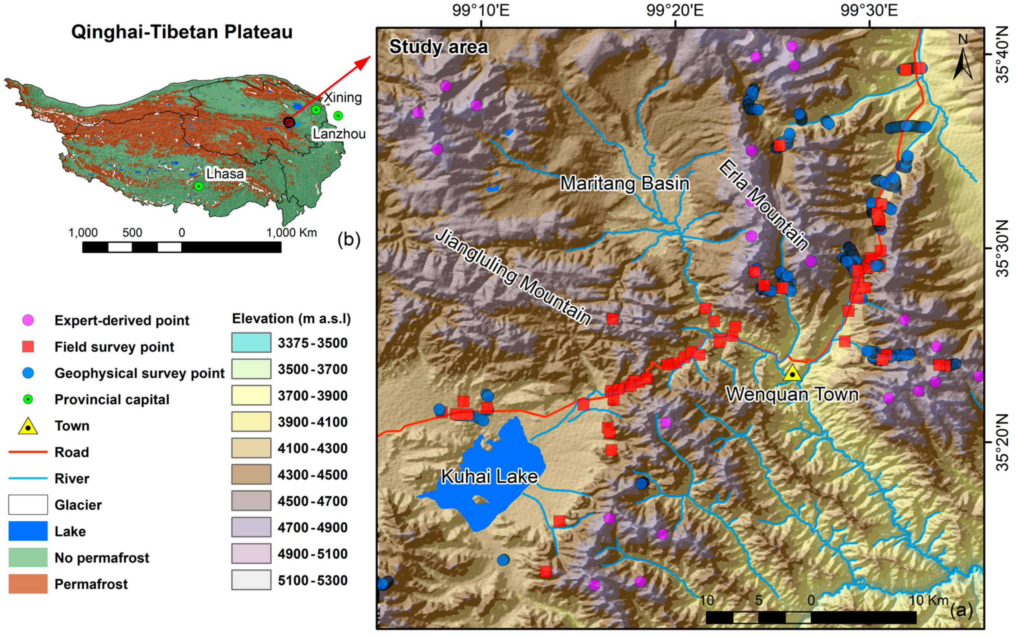
2.1. Study Area and Field Observations

The study was conducted in a mountainous catchment in the upper Yellow River basin, located on the northeastern Qinghai–Tibet Plateau (QTP), China (Figure 1). The region spans elevations from approximately 2000 m to 5000 m and encompasses a mosaic of continuous, discontinuous, sporadic, and seasonally frozen ground. This transitional permafrost zone is influenced by both the East Asian monsoon and midlatitude westerlies, resulting in steep hydrothermal gradients and highly heterogeneous terrain. These characteristics make it an ideal test site for evaluating permafrost mapping methods under complex environmental conditions.
A comprehensive field campaign was conducted in September–October 2009 as part of a national permafrost baseline investigation. Multiple observational techniques were employed, including 73 soil pits, 21 shallow boreholes, and 128 ground-penetrating radar (GPR) transects [31]. The soil pits and boreholes provided point-scale evidence of permafrost presence or absence, while GPR surveys offered spatially continuous subsurface profiles across variable terrain.
GPR data were acquired using a 200 MHz antenna system along transects ranging from 500 m to 3 km in length, covering elevations between 3900 m and 4700 m. The 200 MHz antenna was chosen to balance resolution and penetration depth, with typical detection capabilities reaching 3–5 m under alpine soil conditions. This range is suitable for identifying the upper permafrost boundary, as demonstrated in prior studies [26,27]. Permafrost boundaries were interpreted from reflection horizons and verified against nearby ground-truth sites [26,32]. In total, 956 GPR-based samples were extracted, comprising 702 presence and 254 absence cases.
In addition to the 956 GPR-derived samples and 59 field-observed points from boreholes and pits, we manually selected 22 high-elevation presence samples above 4700 m as empirical constraints to enhance altitudinal representation, based on the established elevation dependence of permafrost and visual interpretation of terrain and landform characteristics. Altogether, 1037 labeled samples (753 presence, 284 absence) were compiled for model development and evaluation.

2.2. Environmental Variables and Data Preprocessing

To characterize the environmental factors influencing permafrost occurrence, we compiled 23 variables spanning three domains: climate, topography, and surface conditions (Table 1). These variables were selected based on their demonstrated relevance in permafrost and cold-region modeling over the Qinghai–Tibet Plateau [14,33,34,35]. All variables are derived from publicly available datasets and were chosen to balance predictive value with physical interpretability. To ensure consistency across heterogeneous spatial datasets, all environmental layers were first projected to a unified Albers equal-area conic coordinate system and then resampled to a 30 m spatial resolution, matching the native resolution of the ASTER GDEM. For continuous variables such as LST, TDD, FDD, and vegetation indices (NDVI, NDWI, NDMI), we applied bilinear interpolation to preserve spatial gradients and reduce smoothing artifacts. For categorical or index-type variables, including Aspect, TWI, and landform masks, we used nearest-neighbor interpolation to maintain class integrity. This preprocessing ensured spatial alignment and comparability across all input features in the modeling framework. Preprocessing steps included reprojection, spatial masking, and normalization. Multi-year means or climatological baselines were used to ensure temporal alignment with the 2009 field campaign.
Climatic variables included land surface temperature (LST), thawing degree days (TDDs), and freezing degree days (FDDs), all derived from MODIS MOD11A1 daily records (2003–2019) at 1 km resolution. Mean annual temperature (AT) and annual precipitation (Pre) were obtained from a 1 km resolution monthly climate dataset developed by Peng et al. [34], which provides downscaled historical climate data over China. These five variables were jointly used to characterize near-surface thermal regimes and long-term hydroclimatic conditions relevant to permafrost occurrence. Topographic variables were extracted from ASTER GDEM v2 (30 m) and include elevation, slope, aspect, topographic wetness index (TWI), and potential solar radiation (Sola). Geographic coordinates (latitude and longitude) were retained to represent large-scale climatic gradients. These terrain-related variables influence energy balance, moisture redistribution, and snow cover retention.
Surface condition variables describe vegetation cover and soil physical properties. NDVI, NDMI, and NDWI were derived from Landsat 8 OLI imagery (30 m resolution, 2013–2015). Although these products postdate the field campaign, prior studies suggest minimal decadal change in alpine vegetation patterns, supporting their use in cold regions [15,30]. However, we note that localized, non-linear vegetation changes driven by warming and land use disturbances may have occurred, potentially introducing uncertainty in the derived indices. Soil variables—including bulk density (Bd), sand (Snd), clay (Clay), gravel content (Cf), and organic carbon density (Soc)—were obtained from a 250 m resolution soil texture dataset developed by Liu et al. [35], based on over 25,000 profile observations across China. These properties influence thermal conductivity and subsurface water dynamics.

2.3. Machine Learning Modeling and Evaluation

To predict permafrost presence or absence (PYN), we implemented thirteen machine learning (ML) algorithms representing four major categories: (1) tree-based models, (2) boosting-based models, (3) linear and kernel-based classifiers, and (4) other classical algorithms. The model types and their key chara cteristics are summarized in Table 2. All models were implemented in Python 3.8 using the Scikit-learn, XGBoost, LightGBM, and CatBoost libraries. Each model was embedded into a pipeline and optimized via grid search using algorithm-specific hyperparameter ranges. For example, Random Forest (RF) and Extremely Randomized Trees (ETs) were tuned for tree depth and the number of estimators; boosting models for learning rate and regularization; SVM for kernel and penalty settings; and neural networks for hidden layer structure and activation functions.
Model training and evaluation followed a stratified 5-fold cross-validation scheme repeated 40 times to enhance stability and robustness. This resulted in 200 train–validation iterations per model. Class stratification maintained the original class ratio (62.7% positive, 37.3% negative) within each fold. For tree-based models, out-of-bag (OOB) estimates were additionally used to assess generalization performance. Z-score normalization was applied to models sensitive to feature scale, such as SVM and logistic regression. Eight evaluation metrics were used to quantify classification performance: accuracy, precision, recall, F1 score, Cohen’s kappa, Matthews correlation coefficient (MCC), area under the receiver operating characteristic curve (AUC-ROC), and area under the precision–recall curve (AUC-PR). The definitions and formulae of these metrics are listed in Table 3.
To interpret variable effects and improve model transparency, SHapley Additive exPlanations (SHAPs) were applied to selected tree-based models. SHAP values were computed using the TreeExplainer module (SHAP v0.47) to estimate the marginal contribution of each input feature. This method provides locally accurate and globally consistent interpretations of variable importance for ensemble decision trees [28]. While these components have been individually applied in previous studies, their combination in a reproducible and physically interpretable workflow offers a novel contribution to cold-region geospatial modeling.

3. Results

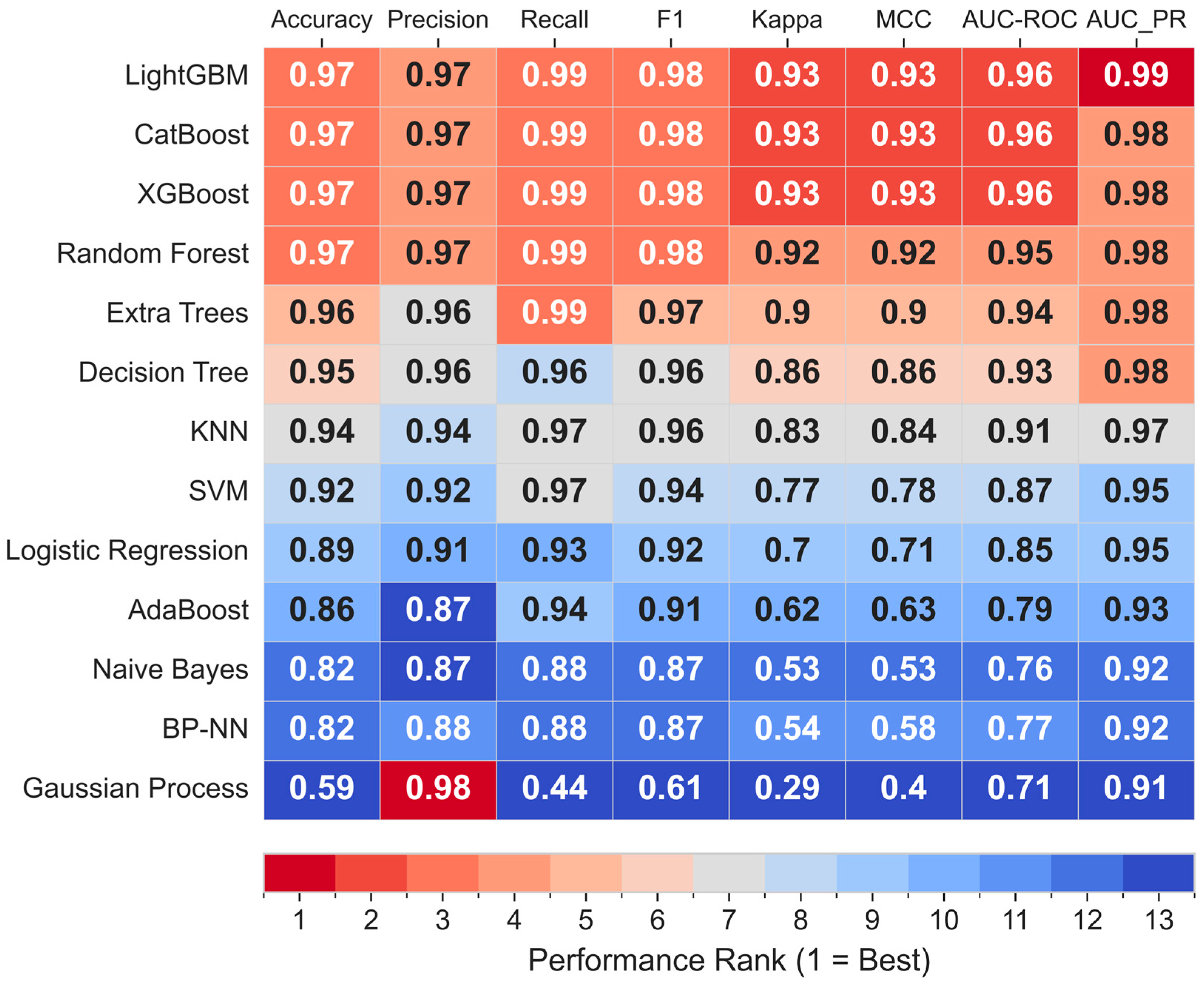
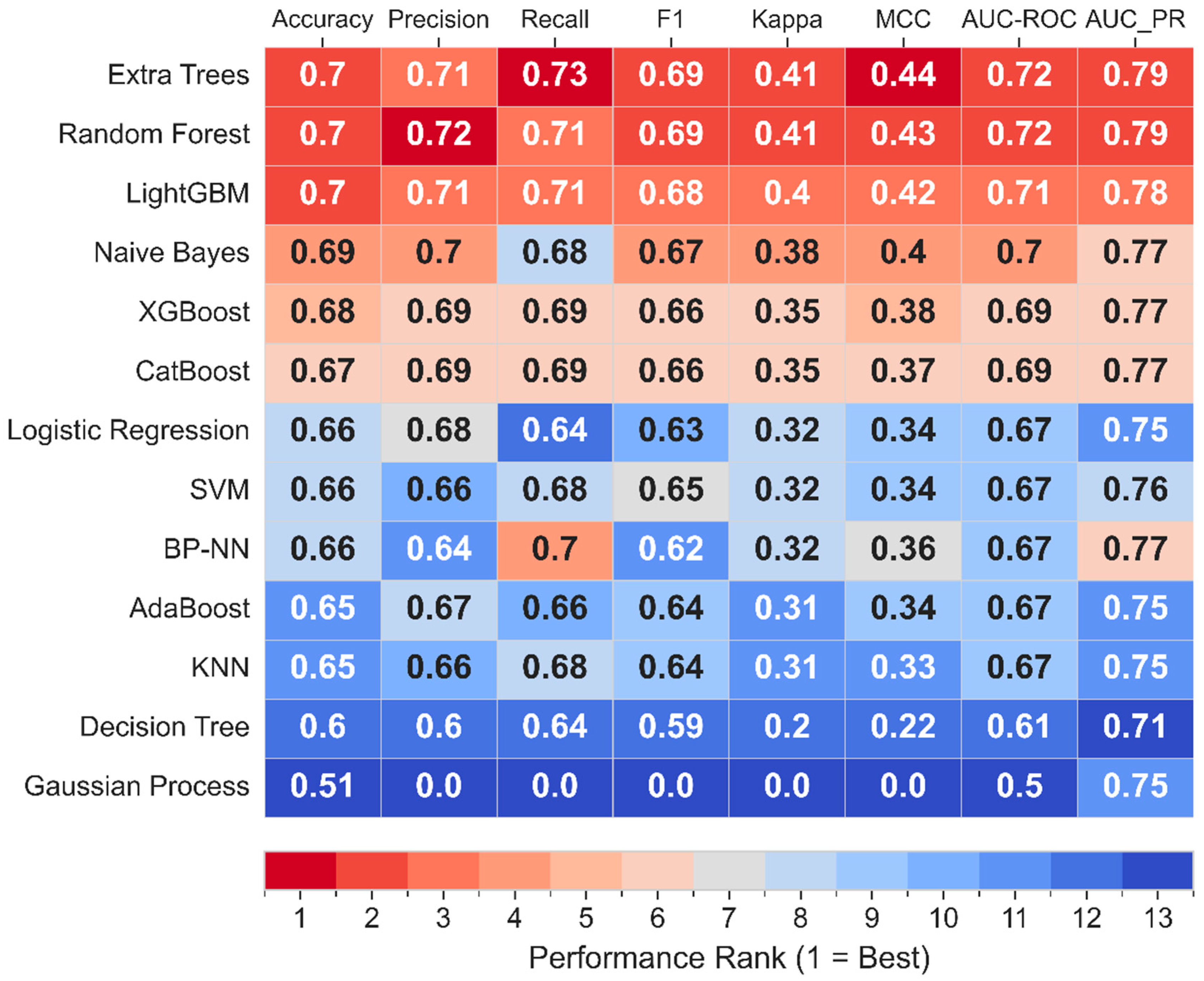
3.1. Model Performance Comparison of 13 Algorithms

The classification performance of thirteen machine learning models was evaluated using repeated cross-validation. Figure 2 summarizes their relative rankings across eight performance metrics. Ensemble tree-based models—particularly LightGBM, CatBoost, XGBoost, and RF—achieved consistently strong results, ranking among the top across nearly all metrics. These models demonstrated high F1 scores (0.98), MCC, and Cohen’s kappa values exceeding 0.93, and an AUC-ROC above 0.96. Among them, LightGBM showed the most stable and balanced performance, ranking first in five of the eight metrics. CatBoost and XGBoost also performed robustly, with slight variations across individual metrics. RF displayed high classification accuracy but relatively lower AUC-ROC. In contrast, classical models such as SVM, logistic regression, and Gaussian process showed weaker performance, particularly in metrics sensitive to class imbalance (e.g., MCC and AUC-PR). Although these top models exhibited similar accuracy levels, their detailed metric profiles reveal nuanced differences in classification behavior. Therefore, we further compared the predicted permafrost distributions from the top four models to assess their spatial generalization capabilities.

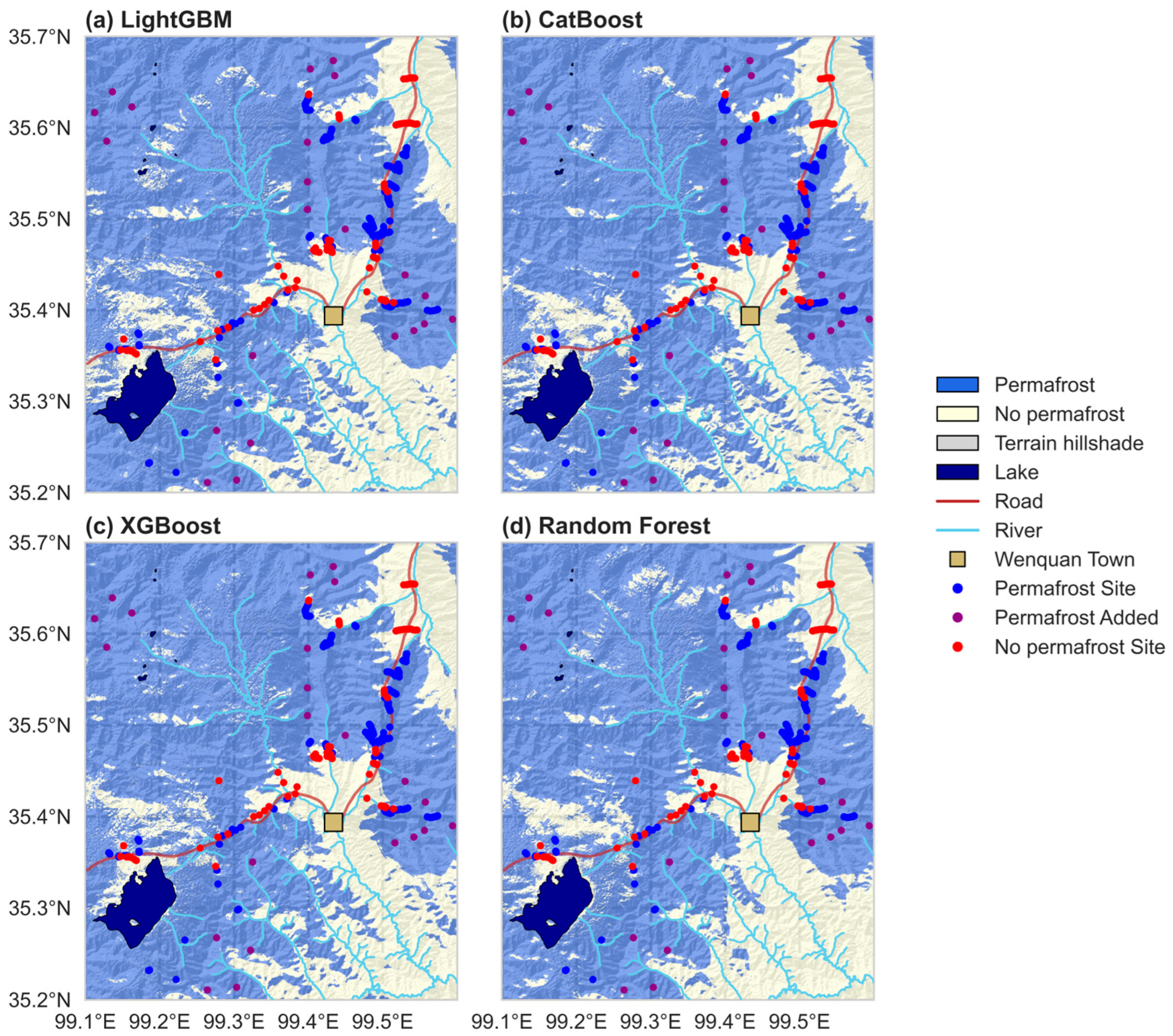
3.2. Spatial Prediction Comparison of the Top Models

To evaluate how model accuracy translates into spatial prediction, we compared the permafrost distribution maps generated by the four best-performing models (LightGBM, CatBoost, XGBoost, and RF) at 30 m resolution (Figure 3). All models captured the broad elevation dependence of mountain permafrost, with predicted presence largely concentrated between 4000 m and 5000 m. However, differences emerged in the continuity and boundary precision of predicted distributions. LightGBM, CatBoost, and XGBoost produced smoother and more spatially coherent patterns, whereas RF yielded more fragmented results, particularly in transitional zones and along south-facing slopes.
Notably, in the 5000–5500 m elevation band—where no original borehole or GPR training data were available—all models predicted nearly complete permafrost coverage (99.98%), as shown in Table 4. This consistency suggests that the inclusion of 22 manually selected high-elevation presence points effectively strengthened the upper bound extrapolation. In the 4500–5000 m zone, CatBoost predicted the highest permafrost proportion (97.58%), followed by Random Forest (96.63%), XGBoost (95.59%), and LightGBM (94.83%). Although differences among models were small in this band, LightGBM produced more spatially continuous and terrain-consistent outputs across the landscape. At mid-elevations (4000–4500 m), which account for 63.6% of the terrain and contain the majority of observations, permafrost coverage ranged from 65.18% to 70.12% across models. In contrast, all models predicted less than 3% permafrost presence below 4000 m, aligning with the observed lower limit and supporting the modeled altitudinal sensitivity (Table 4).

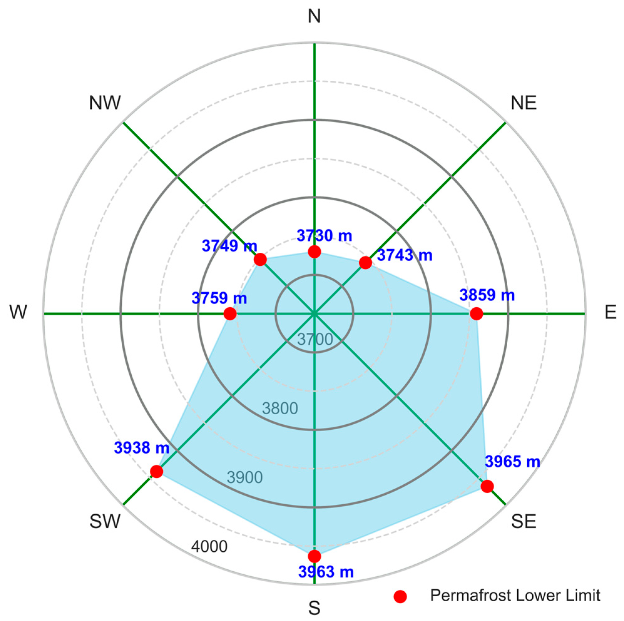
3.3. Aspect-Dependent Lower Elevation Limits of Modeled Permafrost

In mountain permafrost environments, the lower elevation limit marks the climatic boundary below which permafrost can no longer persist. This threshold is sensitive to local microclimatic factors—particularly aspect—and serves as an indicator of terrain–climate interactions. To examine the role of slope orientation, we extracted the minimum elevation at which permafrost was predicted in each of eight aspect sectors, using the LightGBM model. Aspect classes were defined at 45° intervals, with the north-facing sector covering 337.5° to 22.5° (Figure 4). The results reveal clear directional asymmetries. On north-facing slopes (N, NE, NW), modeled permafrost did not appear below ~3730 m, while on south-facing slopes (S, SE, SW), the minimum elevation extended down to 3963 m. This pattern reflects the influence of differential solar radiation: south-facing slopes receive greater incoming energy, which raises the local thermal threshold for permafrost persistence. Although observational data were limited at higher elevations, the predicted aspect-dependent limits align with known microclimatic effects and suggest that the model effectively captures the influence of terrain controls on permafrost boundaries.

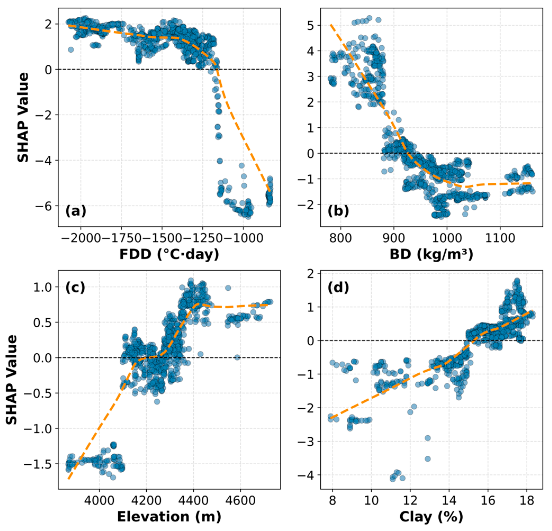
3.4. Feature Contributions Interpreted by SHAP in the LightGBM Model

To interpret the LightGBM classifier and assess variable importance, SHAP analysis was applied to quantify the marginal contribution of each predictor. As shown in Figure 5a, land surface temperature (LST), freezing degree days (FDDs), bulk density (BD), and thawing degree days (TDDs) were the four most important variables, contributing 15.4%, 14.5%, 13.3%, and 10.5% of the total SHAP values, respectively. These variables reflect key climatic and subsurface conditions relevant to permafrost occurrence. The grouped contribution plot (Figure 5b) further indicates that climate-related predictors accounted for 46.5% of the total contribution, followed by surface conditions (31.3%) and topographic factors (22.2%). These group-wise proportions suggest that temperature indices and substrate properties dominate over terrain geometry in determining model outputs.
Figure 6 presents the SHAP dependence relationships for four key variables. FDD showed a threshold-like effect, with SHAP values declining rapidly when values exceeded approximately −1250 °C·day (Figure 6a). BD exhibited a nonlinear negative relationship (Figure 6b), while elevation showed a relatively linear positive contribution within the 3900–4500 m range (Figure 6c). Clay content presented a segmented pattern, with SHAP values increasing more prominently above 15% (Figure 6d). BD also showed a notable change in SHAP response around 910 kg/m3. These variable-specific patterns suggest that the model captured structured, non-linear responses along key environmental gradients.

4. Discussion

4.1. Comparison with Previous Studies

Permafrost distribution mapping on QTP has traditionally relied on empirical indicators such as elevation, air temperature, or vegetation proxies [13,14,36]. These models, while useful at continental scales, often assume fixed threshold relationships and lack the capacity to capture environmental heterogeneity in mountainous terrain. For instance, widely used zonation schemes based on mean annual ground temperature or TTOP models tend to underrepresent topographic and soil-related influences, limiting their applicability at landscape scale [37].
Our model framework, by contrast, incorporates multiple environmental domains—climate, soil, terrain, and vegetation—within a machine learning (ML) structure capable of capturing non-linear interactions. This multi-factor approach enables finer spatial representation and improved adaptability across elevation and slope gradients. In particular, ensemble-based algorithms such as LightGBM demonstrated more consistent performance in complex terrain, as supported by recent studies applying ML to permafrost prediction [38,39,40]. To further enhance performance in data-sparse high-elevation areas, we included 22 presence points above 4700 m as empirical constraints. This supplementation led to more realistic elevation gradients and aspect-dependent permafrost boundaries, underscoring the value of targeted data enhancement in cold-region ML applications.
Moreover, the integration of SHAP analysis provides a critical advancement beyond black-box ML applications. Instead of relying on model coefficients or assumed functional forms, SHAP allows interpretation of variable-specific effects and their interactions (Figure 6), which is especially important in permafrost systems influenced by coupled thermal–hydrological–geomorphic processes. The ability to detect spatially coherent patterns—such as aspect-modulated permafrost limits (Figure 5)—offers new potential for building transparent, decision-supportive models for cryosphere monitoring and infrastructure planning.

4.2. Added Value of GPR-Augmented Training Data

To improve training data representativeness across terrain gradients, we supplemented borehole records with GPR-derived thaw depth measurements (Figure 1). The additional GPR samples expanded coverage in high-elevation, shaded, and roadless areas, reducing sampling bias and enhancing the diversity of environmental conditions represented. The use of GPR in permafrost mapping has been validated in various alpine regions [26,27,31,32,41,42]. In our application, models trained with GPR-augmented data produced more terrain-adaptive and continuous predictions, particularly in transitional zones where borehole-only models tended to underrepresent permafrost (Figure 6). To quantify this improvement, we conducted a parallel experiment using only the 59 field survey samples (soil pits and boreholes). As shown in Figure 7, the classification performance of all top four models (LightGBM, CatBoost, XGBoost, and RF) dropped substantially relative to their GPR-augmented counterparts in Figure 2. Accuracy values fell to approximately 70%, accompanied by reductions across all major metrics, including F1 score, MCC, and AUC-PR. These results highlight the limitations of sparse training data in capturing spatial heterogeneity, particularly in mountainous terrain. The inclusion of GPR samples significantly improved the representativeness of training data, which proved critical for generalizing across heterogeneous terrain.

4.3. Feature Contributions and Environmental Controls

SHAP-based interpretation revealed that Climate variables dominated model responses, with LST, FDD, and TDD jointly accounting for nearly half of the total contribution. These variables represent cumulative thermal inputs and losses over seasonal timescales, reinforcing findings from previous pan-QTP studies [39,43]. However, beyond these known drivers, our results reveal additional layer-specific patterns.
Soil properties—particularly BD and clay content—exhibited threshold-like responses not captured by linear correlation alone. As shown in Figure 6b,d, BD showed a negative contribution shift near ~910 kg/m3, while clay contribution increased more rapidly above 15%. These nonlinear effects reflect their role in regulating thermal conductivity and water retention, aligning with hydrothermal coupling processes previously reported [44,45]. Topographic influence, though secondary in total contribution, introduced spatial asymmetry. Aspect significantly modulated the lower elevation limit of predicted permafrost (Figure 4), consistent with solar radiation patterns [15,30,31]. While elevation displayed a quasi-linear SHAP trend across 3900–4500 m (Figure 6c), its predictive role was likely confounded by snow accumulation and radiation exposure.
In addition, Figure 6a shows a sharp decline in FDD’s marginal contribution above ~–1250 °C·day, suggesting a possible climatic threshold below which permafrost becomes increasingly unlikely. Such thresholds provide valuable cues for future model-based extrapolation and for identifying tipping points under warming scenarios [46,47]. These results reinforce the need to jointly consider thermal, edaphic, and geomorphic controls when analyzing permafrost regimes.

4.4. Limitations and Outlook

This study relies on multi-source datasets that vary in spatial resolution and acquisition time. Some remote sensing variables, such as NDMI and NDVI, were derived from multi-year means (2013–2015), whereas other key predictors like LST and FDD were based on longer-term MODIS records (2003–2019). GPR observations were collected in 2009. Although this temporal offset was mitigated by focusing on stable land surface properties, minor inconsistencies cannot be fully excluded. In evaluating model performance, we observed that high cross-validation scores did not always translate into reliable spatial predictions, particularly in high-elevation or extrapolated zones. Recognizing this limitation, we incorporated the elevation dependence of permafrost into our assessment, which enabled the identification of models with stronger terrain sensitivity. This result supports recent findings that emphasize the need to complement statistical metrics with physical reasoning or empirical thresholds when selecting and interpreting machine learning models for geospatial applications [48,49,50].
Looking forward, future studies could benefit from integrating additional physical constraints, such as slope–aspect-adjusted thresholds or monotonic elevation trends, into both model evaluation and post-processing. Combining data-driven algorithms with empirical rules or process-based filters may enhance the robustness, realism, and transferability of permafrost predictions under changing climate conditions. Furthermore, while repeated cross-validation offers a robust internal estimate of model performance, our evaluation did not include an independent spatial or temporal test set. This limits the full assessment of the model’s generalizability to unseen regions or conditions. Future work should incorporate spatially or temporally independent validation datasets—collected from different locations or time periods—to rigorously evaluate extrapolation capabilities and enhance confidence in large-scale deployment.

5. Conclusions

This study developed a high-resolution permafrost mapping framework by integrating GPR-augmented field observations with machine learning and SHAP-based interpretation. Using 1037 permafrost samples and 20 environmental predictors, we evaluated 13 classification algorithms and demonstrated that RF, LightGBM, CatBoost, and XGBoost achieved consistently high performance. In particular, cross-validation results showed that all top-performing models achieved average classification accuracies exceeding 97% within the training domain. Among them, LightGBM showed the strongest terrain adaptability and best preserved the altitudinal dependency of permafrost presence. The addition of empirically constrained high-altitude samples significantly improved model generalization, particularly in topographically complex and data-sparse regions.
SHAP analysis revealed that climate variables—especially LST, FDD, and TDD—were the most influential predictors, followed by soil-related factors such as BD and clay. Together, climate and soil variables contributed nearly 80% to model outputs. Several key predictors exhibited nonlinear or threshold-like responses, confirming their physical relevance. The modeled permafrost lower limit occurred near 4000 m, with over 94% predicted coverage above 4500 m and nearly full coverage in results above 5000 m. The elevation threshold varied by over 200 m across slope aspects, indicating strong topographic modulation. Additional comparative experiments showed that incorporating GPR-derived samples significantly improved model accuracy and generalization, particularly in high-altitude and data-sparse regions.
Despite existing limitations in temporal consistency, input resolution, and high-altitude sampling, the proposed model offers a robust, interpretable, and scalable approach to mountain permafrost mapping. This framework can be readily extended to other regions by incorporating localized observations and provides valuable support for environmental monitoring and infrastructure risk assessment in cryospheric environments.

Author Contributions

Conceptualization, Y.X., G.L. and L.Z.; methodology, Y.X. and G.H.; software, Y.X. and D.Z.; validation, R.L. and E.D.; formal analysis, Y.X.; resources, G.H.; data curation, G.L.; writing—original draft preparation, Y.X. and G.L.; writing—review and editing, T.W., X.W. and L.Z.; visualization, G.Z. and Y.Z.; funding acquisition, G.H. and L.Z. All authors have read and agreed to the published version of the manuscript.

Funding

This work was financially supported by the National Key Research and Development Program of China (2022YFF0711702), the National Natural Science Foundation of China (42322608, 42471168), the program of the Key Laboratory of Cryospheric Science and Frozen Soil Engineering, CAS (No. CSFSE-ZQ-2405, CSFSE-ZQ-2407 and CSFSE-ZZ-2408), and the Youth Innovation Promotion Association of the Chinese Academy of Sciences (2022430).

Data Availability Statement

All environmental variables used in this study were derived from publicly accessible datasets. Climatic data were obtained from the MODIS MOD11A1 product (https://doi.org/10.5067/MODIS/MOD11A1.061, accessed on 5 March 2025). Mean annual temperature and precipitation data were obtained from a 1 km gridded dataset developed by Peng et al. [34], accessible via the National Tibetan Plateau Data Center (http://data.tpdc.ac.cn, accessed on 5 March 2025). Topographic variables were derived from the ASTER GDEM v2 (https://asterweb.jpl.nasa.gov/gdem.asp, accessed on 5 March 2025), and vegetation indices (NDVI, NDWI, NDMI) were calculated from Landsat 8 OLI surface reflectance data (https://earthexplorer.usgs.gov/, accessed on 5 March 2025). Soil property data were derived from a 250 m resolution national dataset developed by Liu et al. [35], available at the National Tibetan Plateau Data Center (http://data.tpdc.ac.cn, accessed on 5 March 2025). All analyses were conducted in Python 3.9.21 using scikit-learn 1.6.1, LightGBM 4.5.0, XGBoost 2.1.4, CatBoost 1.2.7, and shap 0.46.0.

Acknowledgments

The authors appreciate all the data provided by each open database. The authors thank the anonymous reviewers and academic editors for their comments.

Conflicts of Interest

The authors declare no conflicts of interest.

References

  1. Hugelius, G.; Loisel, J.; Chadburn, S.; Jackson, R.B.; Jones, M.; MacDonald, G.; Marushchak, M.; Olefeldt, D.; Packalen, M.; Siewert, M.B.; et al. Large Stocks of Peatland Carbon and Nitrogen Are Vulnerable to Permafrost Thaw. Proc. Natl. Acad. Sci. USA 2020, 117, 20438–20446. [Google Scholar] [CrossRef] [PubMed]
  2. Vonk, J.E.; Tank, S.E.; Bowden, W.B.; Laurion, I.; Vincent, W.F.; Alekseychik, P.; Amyot, M.; Billet, M.F.; Canário, J.; Cory, R.M.; et al. Reviews and Syntheses: Effects of Permafrost Thaw on Arctic Aquatic Ecosystems. Biogeosciences 2015, 12, 7129–7167. [Google Scholar] [CrossRef]
  3. Zhang, T. Influence of the Seasonal Snow Cover on the Ground Thermal Regime: An Overview. Rev. Geophys. 2005, 43, 2004RG000157. [Google Scholar] [CrossRef]
  4. Miner, K.R.; Turetsky, M.R.; Malina, E.; Bartsch, A.; Tamminen, J.; McGuire, A.D.; Fix, A.; Sweeney, C.; Elder, C.D.; Miller, C.E. Permafrost Carbon Emissions in a Changing Arctic. Nat. Rev. Earth Environ. 2022, 3, 55–67. [Google Scholar] [CrossRef]
  5. Turetsky, M.R.; Abbott, B.W.; Jones, M.C.; Anthony, K.W.; Olefeldt, D.; Schuur, E.A.G.; Grosse, G.; Kuhry, P.; Hugelius, G.; Koven, C.; et al. Carbon Release through Abrupt Permafrost Thaw. Nat. Geosci. 2020, 13, 138–143. [Google Scholar] [CrossRef]
  6. Biskaborn, B.K.; Smith, S.L.; Noetzli, J.; Matthes, H.; Vieira, G.; Streletskiy, D.A.; Schoeneich, P.; Romanovsky, V.E.; Lewkowicz, A.G.; Abramov, A.; et al. Permafrost Is Warming at a Global Scale. Nat. Commun. 2019, 10, 264. [Google Scholar] [CrossRef]
  7. Smith, S.L.; O’Neill, H.B.; Isaksen, K.; Noetzli, J.; Romanovsky, V.E. The Changing Thermal State of Permafrost. Nat. Rev. Earth Environ. 2022, 3, 10–23. [Google Scholar] [CrossRef]
  8. Liljedahl, A.K.; Boike, J.; Daanen, R.P.; Fedorov, A.N.; Frost, G.V.; Grosse, G.; Hinzman, L.D.; Iijma, Y.; Jorgenson, J.C.; Matveyeva, N.; et al. Pan-Arctic Ice-Wedge Degradation in Warming Permafrost and Its Influence on Tundra Hydrology. Nat. Geosci. 2016, 9, 312–318. [Google Scholar] [CrossRef]
  9. Mu, C.; Abbott, B.W.; Norris, A.J.; Mu, M.; Fan, C.; Chen, X.; Jia, L.; Yang, R.; Zhang, T.; Wang, K.; et al. The Status and Stability of Permafrost Carbon on the Tibetan Plateau. Earth Sci. Rev. 2020, 211, 103433. [Google Scholar] [CrossRef]
  10. Peng, X.; Zhang, T.; Frauenfeld, O.W.; Mu, C.; Wang, K.; Wu, X.; Guo, D.; Luo, J.; Hjort, J.; Aalto, J.; et al. Active Layer Thickness and Permafrost Area Projections for the 21st Century. Earth’s Future 2023, 11, e2023EF003573. [Google Scholar] [CrossRef]
  11. Wang, T.; Yang, D.; Yang, Y.; Zheng, G.; Jin, H.; Li, X.; Yao, T.; Cheng, G. Pervasive Permafrost Thaw Exacerbates Future Risk of Water Shortage Across the Tibetan Plateau. Earth’s Future 2023, 11, e2022EF003463. [Google Scholar] [CrossRef]
  12. Nicolsky, D.J.; Romanovsky, V.E. Modeling Long-term Permafrost Degradation. J. Geophys. Res. Earth Surf. 2018, 123, 1756–1771. [Google Scholar] [CrossRef]
  13. Obu, J.; Westermann, S.; Bartsch, A.; Berdnikov, N.; Christiansen, H.H.; Dashtseren, A.; Delaloye, R.; Elberling, B.; Etzelmüller, B.; Kholodov, A.; et al. Northern Hemisphere Permafrost Map Based on TTOP Modelling for 2000–2016 at 1 km2 Scale. Earth Sci. Rev. 2019, 193, 299–316. [Google Scholar] [CrossRef]
  14. Zou, D.; Zhao, L.; Sheng, Y.; Chen, J.; Hu, G.; Wu, T.; Wu, J.; Xie, C.; Wu, X.; Pang, Q.; et al. A New Map of Permafrost Distribution on the Tibetan Plateau. Cryosphere 2017, 11, 2527–2542. [Google Scholar] [CrossRef]
  15. Boeckli, L.; Brenning, A.; Gruber, S.; Noetzli, J. Permafrost Distribution in the European Alps: Calculation and Evaluation of an Index Map and Summary Statistics. Cryosphere 2012, 6, 807–820. [Google Scholar] [CrossRef]
  16. Deluigi, N.; Lambiel, C.; Kanevski, M. Data-Driven Mapping of the Potential Mountain Permafrost Distribution. Sci. Total Environ. 2017, 590–591, 370–380. [Google Scholar] [CrossRef]
  17. Sun, W.; Cao, B.; Hao, J.; Wang, S.; Clow, G.D.; Sun, Y.; Fan, C.; Zhao, W.; Peng, X.; Yao, Y.; et al. Two-Dimensional Simulation of Island Permafrost Degradation in Northeastern Tibetan Plateau. Geoderma 2023, 430, 116330. [Google Scholar] [CrossRef]
  18. Tahmasebi, P.; Kamrava, S.; Bai, T.; Sahimi, M. Machine Learning in Geo- and Environmental Sciences: From Small to Large Scale. Adv. Water Resour. 2020, 142, 103619. [Google Scholar] [CrossRef]
  19. Ran, Y.; Li, X.; Cheng, G. Climate Warming over the Past Half Century Has Led to Thermal Degradation of Permafrost on the Qinghai–Tibet Plateau. Cryosphere 2018, 12, 595–608. [Google Scholar] [CrossRef]
  20. Wang, X.; Ran, Y.; Pang, G.; Chen, D.; Su, B.; Chen, R.; Li, X.; Chen, H.W.; Yang, M.; Gou, X.; et al. Contrasting Characteristics, Changes, and Linkages of Permafrost between the Arctic and the Third Pole. Earth-Sci. Rev. 2022, 230, 104042. [Google Scholar] [CrossRef]
  21. Baral, P.; Haq, M.A. Spatial Prediction of Permafrost Occurrence in Sikkim Himalayas Using Logistic Regression, Random Forests, Support Vector Machines and Neural Networks. Geomorphology 2020, 371, 107331. [Google Scholar] [CrossRef]
  22. Li, X.; Ji, Y.; Zhou, G.; Zhou, L.; Li, X.; He, X.; Tian, Z. A New Method for Bare Permafrost Extraction on the Tibetan Plateau by Integrating Machine Learning and Multi-Source Information. Remote Sens. 2023, 15, 5328. [Google Scholar] [CrossRef]
  23. Popescu, R.; Filhol, S.; Etzelmüller, B.; Vasile, M.; Pleșoianu, A.; Vîrghileanu, M.; Onaca, A.; Șandric, I.; Săvulescu, I.; Cruceru, N.; et al. Permafrost Distribution in the Southern Carpathians, Romania, Derived from Machine Learning Modeling. Permafr. Periglac. Process. 2024, 35, 243–261. [Google Scholar] [CrossRef]
  24. Șerban, R.-D.; Șerban, M.; He, R.; Jin, H.; Li, Y.; Li, X.; Wang, X.; Li, G. 46-Year (1973–2019) Permafrost Landscape Changes in the Hola Basin, Northeast China Using Machine Learning and Object-Oriented Classification. Remote Sens. 2021, 13, 1910. [Google Scholar] [CrossRef]
  25. Sheng, Q.; Zhang, Y.; Li, K.; Ling, X.; Li, J. Exploring the Seasonal Comparison of Land Surface Temperature Dominant Factors in the Tibetan Plateau. ISPRS Ann. Photogramm. Remote Sens. Spat. Inf. Sci. 2024, X-1-2024, 197–203. [Google Scholar] [CrossRef]
  26. Cao, B.; Gruber, S.; Zhang, T.; Li, L.; Peng, X.; Wang, K.; Zheng, L.; Shao, W.; Guo, H. Spatial Variability of Active Layer Thickness Detected by Ground-penetrating Radar in the Qilian Mountains, Western China. J. Geophys. Res. Earth Surf. 2017, 122, 574–591. [Google Scholar] [CrossRef]
  27. Du, E.; Zhao, L.; Zou, D.; Li, R.; Wang, Z.; Wu, X.; Hu, G.; Zhao, Y.; Liu, G.; Sun, Z. Soil Moisture Calibration Equations for Active Layer GPR Detection—A Case Study Specially for the Qinghai–Tibet Plateau Permafrost Regions. Remote Sens. 2020, 12, 605. [Google Scholar] [CrossRef]
  28. Lundberg, S.M.; Erion, G.; Chen, H.; DeGrave, A.; Prutkin, J.M.; Nair, B.; Katz, R.; Himmelfarb, J.; Bansal, N.; Lee, S.-I. From Local Explanations to Global Understanding with Explainable AI for Trees. Nat. Mach. Intell. 2020, 2, 56–67. [Google Scholar] [CrossRef]
  29. Zhong, S.; Zhang, K.; Bagheri, M.; Burken, J.G.; Gu, A.; Li, B.; Ma, X.; Marrone, B.L.; Ren, Z.J.; Schrier, J.; et al. Machine Learning: New Ideas and Tools in Environmental Science and Engineering. Environ. Sci. Technol. 2021, 55, 12741–12754. [Google Scholar] [CrossRef]
  30. Haberkorn, A.; Kenner, R.; Noetzli, J.; Phillips, M. Changes in Ground Temperature and Dynamics in Mountain Permafrost in the Swiss Alps. Front. Earth Sci. 2021, 9, 626686. [Google Scholar] [CrossRef]
  31. Liu, G.; Zhao, L.; Xie, C.; Zou, D.; Wu, T.; Du, E.; Wang, L.; Sheng, Y.; Zhao, Y.; Xiao, Y.; et al. The Zonation of Mountain Frozen Ground under Aspect Adjustment Revealed by Ground-Penetrating Radar Survey—A Case Study of a Small Catchment in the Upper Reaches of the Yellow River, Northeastern Qinghai–Tibet Plateau. Remote Sens. 2022, 14, 2450. [Google Scholar] [CrossRef]
  32. Angelopoulos, M.C.; Pollard, W.H.; Couture, N.J. The Application of CCR and GPR to Characterize Ground Ice Conditions at Parsons Lake, Northwest Territories. Cold Reg. Sci. Technol. 2013, 85, 22–33. [Google Scholar] [CrossRef]
  33. Yang, J.; Dong, J.; Xiao, X.; Dai, J.; Wu, C.; Xia, J.; Zhao, G.; Zhao, M.; Li, Z.; Zhang, Y.; et al. Divergent Shifts in Peak Photosynthesis Timing of Temperate and Alpine Grasslands in China. Remote Sens. Environ. 2019, 233, 111395. [Google Scholar] [CrossRef]
  34. Peng, S.; Ding, Y.; Liu, W.; Li, Z. 1 Km Monthly Temperature and Precipitation Dataset for China from 1901 to 2017. Earth Syst. Sci. Data 2019, 11, 1931–1946. [Google Scholar] [CrossRef]
  35. Liu, F.; Zhang, G.-L.; Song, X.; Li, D.; Zhao, Y.; Yang, J.; Wu, H.; Yang, F. High-Resolution and Three-Dimensional Mapping of Soil Texture of China. Geoderma 2020, 361, 114061. [Google Scholar] [CrossRef]
  36. Li, S.; Cheng, G. Map of Frozen Ground on Qinghai-Xizang Plateau; Gansu Culture Press: Lanzhou, China, 1996. [Google Scholar]
  37. Li, W.; Weng, B.; Yan, D.; Lai, Y.; Li, M.; Wang, H. Underestimated Permafrost Degradation: Improving the TTOP Model Based on Soil Thermal Conductivity. Sci. Total Environ. 2023, 854, 158564. [Google Scholar] [CrossRef]
  38. Liu, Y.; Ran, Y.; Li, X.; Che, T.; Wu, T. Multisite Evaluation of Physics-Informed Deep Learning for Permafrost Prediction in the Qinghai-Tibet Plateau. Cold Reg. Sci. Technol. 2023, 216, 104009. [Google Scholar] [CrossRef]
  39. Ran, Y.; Li, X.; Cheng, G.; Nan, Z.; Che, J.; Sheng, Y.; Wu, Q.; Jin, H.; Luo, D.; Tang, Z.; et al. Mapping the Permafrost Stability on the Tibetan Plateau for 2005–2015. Sci. China Earth Sci. 2021, 64, 62–79. [Google Scholar] [CrossRef]
  40. Zhang, Y.-Z.; Liang, S.-J.; Chen, J.-B.; Wang, M.; Jia, M.-T.; Jiang, Y.-T. Enhancing Artificial Permafrost Table Predictions Using Integrated Climate and Ground Temperature Data: A Case Study from the Qinghai-Xizang Highway. Cold Reg. Sci. Technol. 2025, 229, 104341. [Google Scholar] [CrossRef]
  41. Shen, Y.; Zuo, R.; Liu, J.; Tian, Y.; Wang, Q. Characterization and Evaluation of Permafrost Thawing Using GPR Attributes in the Qinghai-Tibet Plateau. Cold Reg. Sci. Technol. 2018, 151, 302–313. [Google Scholar] [CrossRef]
  42. Wu, T.; Wang, Q.; Watanabe, M.; Chen, J.; Battogtokh, D. Mapping Vertical Profile of Discontinuous Permafrost with Ground Penetrating Radar at Nalaikh Depression, Mongolia. Environ. Geol. 2009, 56, 1577–1583. [Google Scholar] [CrossRef]
  43. Obu, J. How Much of the Earth’s Surface Is Underlain by Permafrost? J. Geophys. Res. Earth Surf. 2021, 126, e2021JF006123. [Google Scholar] [CrossRef]
  44. Hu, G.; Zhao, L.; Li, R.; Park, H.; Wu, X.; Su, Y.; Guggenberger, G.; Wu, T.; Zou, D.; Zhu, X.; et al. Water and Heat Coupling Processes and Its Simulation in Frozen Soils: Current Status and Future Research Directions. Catena 2023, 222, 106844. [Google Scholar] [CrossRef]
  45. Gao, K.; Tang, Y.; Chen, D.; Wang, J.; Duan, A. Influence of Arctic Sea Ice and Interdecadal Pacific Oscillation on the Recent Increase of Winter Extreme Snowfall in Northeast China. Atmos. Res. 2023, 295, 107030. [Google Scholar] [CrossRef]
  46. Li, R.; Ma, J.; Wu, T.; Wang, Q.; Wu, X.; Zhao, L.; Wang, S.; Hu, G.; Liu, W.; Jiao, Y.; et al. The Spatiotemporal Variations of Freezing Index and Its Relationship with Permafrost Degradation over the Qinghai–Tibet Plateau from 1977 to 2016. Theor. Appl. Clim. 2024, 155, 985–998. [Google Scholar] [CrossRef]
  47. Martin, L.C.P.; Nitzbon, J.; Aas, K.S.; Etzelmüller, B.; Kristiansen, H.; Westermann, S. Stability Conditions of Peat Plateaus and Palsas in Northern Norway. J. Geophys. Res. Earth Surf. 2019, 124, 705–719. [Google Scholar] [CrossRef]
  48. Reichstein, M.; Camps-Valls, G.; Stevens, B.; Jung, M.; Denzler, J.; Carvalhais, N. Prabhat Deep Learning and Process Understanding for Data-Driven Earth System Science. Nature 2019, 566, 195–204. [Google Scholar] [CrossRef]
  49. Beddrich, J.; Gupta, S.; Wohlmuth, B.; Chiogna, G. The Importance of Topographic Gradients in Alpine Permafrost Modeling. Adv. Water Resour. 2022, 170, 104321. [Google Scholar] [CrossRef]
  50. Bergen, K.J.; Johnson, P.A.; De Hoop, M.V.; Beroza, G.C. Machine Learning for Data-Driven Discovery in Solid Earth Geoscience. Science 2019, 363, eaau0323. [Google Scholar] [CrossRef]
Figure 1. Study area and distribution of field and geophysical survey sites. (a) Elevation map of the study area showing field survey points (red squares), GPR-based geophysical survey points (blue circles), and high-elevation permafrost constraint points (purple triangles) manually selected to enhance upper-altitude representation. Major topographic features and infrastructure are also labeled. Permafrost distribution is based on Zou et al. [14], overlaid on a shaded relief map (DEM hillshade) to enhance topographic readability. (b) Regional location of the study area on the Qinghai–Tibet Plateau.
Remotesensing 17 02015 g001
Figure 2. Cross-validated performance of 13 classification models evaluated using eight metrics. Values indicate the mean performance across 200 training–validation splits. Color shading denotes relative rank across models, with lower ranks indicating better performance (1 = best). Key metrics include Accuracy, F1 score, ROC-AUC, and MCC.
Remotesensing 17 02015 g002
Figure 3. Spatial comparison of permafrost predictions from the top four performing models: (a) LightGBM, (b) CatBoost, (c) XGBoost, and (d) Random Forest. Each panel shows binary classification results (permafrost vs. non-permafrost) at 30 m resolution, overlaid on a terrain hillshade background. Colored points represent validation sites. Differences in boundary transitions and localized predictions reflect variations in model generalization.
Remotesensing 17 02015 g003
Figure 4. Aspect-dependent lower elevation limits of permafrost predicted by the LightGBM model. Each red dot represents the minimum elevation of predicted permafrost within a given aspect sector, defined at 45° intervals (e.g., N: 337.5°–22.5°, NE: 22.5°–67.5°, etc.). The shaded area connects these minimum values to illustrate the overall pattern. Solid and dashed rings indicate elevation intervals of 100 m and 50 m, respectively.
Remotesensing 17 02015 g004
Figure 5. SHAP-based interpretation of feature contributions in the LightGBM model. (a) Summary plot of the top-ranked predictors showing their average SHAP values and effect directions. Colors indicate feature values. (b) Grouped contribution analysis based on SHAP values. The inner ring shows individual variable importance, and the outer ring summarizes the relative contributions of three factor categories: climatic (blue), surface condition (green), and topographic (orange).
Remotesensing 17 02015 g005
Figure 6. SHAP dependence plots for key predictors of permafrost in the LightGBM model. Each subplot shows how the SHAP value (y-axis) varies with the original variable value (x-axis), indicating the marginal effect of that variable on the predicted permafrost presence. Dashed lines indicate smoothed LOWESS trends. (a) Freezing degree days (FDDs), (b) bulk density (BD), (c) elevation (DEM), and (d) clay content demonstrate nonlinear and threshold responses, reflecting climatic and soil controls on permafrost presence.
Remotesensing 17 02015 g006
Figure 7. Classification performance of 13 machine learning models trained without GPR-augmented training data. Same as Figure 2.
Remotesensing 17 02015 g007
Table 1. Summary of environmental variables used for permafrost distribution modeling.
VariableCodeDescription/RelevanceData Source
Climatic factors
Land surface temperatureLSTProxy for near-surface energy input and surface heat budgetMODIS MOD11A1 (2003–2019)
Thawing degree daysTDDCumulative thermal energy during thaw season; key driver of permafrost degradationDerived from MODIS
Freezing degree daysFDDAccumulated freezing intensity; indicator of freeze durationDerived from MODIS
Mean annual temperatureATHighly collinear with TDD; retained to enhance climatic contextPeng et al. [34]
Annual precipitationPreReflects hydrothermal conditions; potentially influences vegetation and insulationPeng et al. [34]
Topographic factors
Elevation DEMControls surface temperature and soil water content via lapse rateASTER GDEM v2
Slope SlopeInfluences runoff and snow redistributionDerived from DEM
Aspect AspectAffects solar exposure and snowmelt timingDerived from DEM
Topographic Wetness Index TWIProxy for water accumulation and soil moistureDEM-derived
Solar radiation SolaControls energy input; relevant for melt and insulation processesGIS-based solar model
Latitude LatProxy for regional climate gradientASTER
Longitude LonCaptures east–west climatic and vegetative differencesASTER
Surface condition factors
Normalized Difference Vegetation Index NDVIProxy for vegetation cover; alters insulation and latent heat fluxLandsat 8 (2013–2015)
Normalized Difference Water Index NDWIIndicator of surface water content and wetnessLandsat 8 (2013–2015)
Normalized Difference Moisture Index NDMIProxy for canopy and surface moistureLandsat 8 (2013–2015)
Bulk densityBDKey determinant of soil thermal conductivityLiu et al. [35]
Sand contentSndAffects porosity, drainage, and freeze–thaw dynamics
Clay contentClayInfluences heat capacity and moisture retention
Organic carbon densitySocRelated to soil insulation and carbon storage; collinear with BD in some cases
Gravel fraction CfImpacts soil heat flux and infiltration pathways
Table 2. Categories and key characteristics of the 13 machine learning models.
CategoryAbbreviationModel NameKey Characteristics
Tree-Based ModelsRFRandom Forest Ensemble of decision trees based on bagging; robust to overfitting and handles high-dimensional data effectively.
ETExtremely Randomized TreesSimilar to RF but with more randomized splits; faster training and reduced variance.
DTDecision TreeSingle-tree structure; highly interpretable but prone to overfitting on complex datasets.
Boosting-Based Models (GBDT)XGBoostExtreme Gradient BoostingHighly efficient; incorporates advanced regularization techniques to prevent overfitting; excels in handling large datasets with complex patterns.
LightGBMLight Gradient Boosting MachineOptimized for speed and memory efficiency; uses histogram-based learning; particularly suitable for large dataset.
CatBoostCatBoostSpecifically designed for categorical feature encoding and high performance; reduces the need for extensive preprocessing.
AdaBoostAdaptive BoostingUsing weighted weak classifiers to improve overall prediction accuracy.
Linear and Kernel-Based ModelsLRLogistic RegressionLinear model for binary classification; simple, interpretable, and works well with linearly separable data.
SVMSupport Vector MachineKernel-based method for both linear and nonlinear classification; effective for small dataset with clear margins of separations.
GPGaussian ProcessProbabilistic non-parametric Bayesian model; provides uncertainty estimates but computationally expensive.
Other ModelsBP-NNBP Neural NetworkMulti-layer perceptron; a classical neural network; suitable for capturing complex, nonlinear relationships in data.
KNNK-Nearest NeighborsNon-parametric model relying on distance measures; sensitive to the choice of k and feature scaling.
NBNaive BayesSimple probabilistic classifier based on Bayes’ theorem; assumes feature independence; included as a baseline for evaluating model performance in structured environmental data.
Table 3. Performance metrics and formulae for evaluating classification accuracy.
Performance ParametersFormulaDescription
Accuracy A c c u r a c y = T P + T N T P + F P + T N + F N The proportion of correctly classified samples among all samples, reflecting the overall predictive capability.
Precision P r e c i s i o n = T P T P + F P The proportion of predicted positive samples that are true positives.
Recall R e c a l l = T P T P + F N The proportion of actual positive samples correctly identified.
F1 Score F 1 = 2 · P r e c i s i o n · R e c a l l P r e c i s i o n + R e c a l l The harmonic mean of precision and recall, balancing both metrics.
Cohen’s Kappa κ = P o P e 1 P e Measures agreement between predicted and observed classifications, considering chance agreement.
MCC M C C = T P × T N F P × F N ( T P + F P ) ( T P + F N ) ( T N + F P ) ( T N + F N ) A balanced metric considering all four confusion matrix elements, suitable for imbalanced data.
AUC-ROC A U C = 0 1 T P R ( F P R ) d F P R Area under the ROC curve, measuring the ability to distinguish between positive and negative classes.
AUC-PR A U C - P R = 0 1 P r e c i s i o n ( R e c a l l ) d R e c a l l Area under the precision–recall curve, particularly useful for evaluating imbalanced data.
Notes: TP (true positives), TN (true negatives), FP (false positives), FN (false negatives), Po (observed agreement), Pe (expected agreement by chance).
Table 4. Elevation-based comparison of terrain area, observation site density, and predicted permafrost proportion across models.
Elevation BandArea Proportion (%)Observation SitesPermafrost Proportion (%)
LightGBMCatBoostXGBoostRandom Forest
3000–3500 m0.0700000
3500–4000 m7.79400.792.661.740
4000–4500 m63.6492765.2768.2870.1265.18
4500–5000 m28.354894.8397.5895.5996.63
5000–5500 m0.16099.9899.9899.9899.98
Note: “Permafrost Proportion (%)” refers to the percentage of grid cells within each elevation band predicted as permafrost.
Disclaimer/Publisher’s Note: The statements, opinions and data contained in all publications are solely those of the individual author(s) and contributor(s) and not of MDPI and/or the editor(s). MDPI and/or the editor(s) disclaim responsibility for any injury to people or property resulting from any ideas, methods, instructions or products referred to in the content.

