Article

Reconstruction of Three-Dimensional Temperature and Salinity in the Equatorial Ocean with Deep-Learning

1
School of Marine Sciences, Sun Yat-sen University, Zhuhai 519082, China
2
Laoshan Laboratory, Qingdao 266237, China
*
Author to whom correspondence should be addressed.
Remote Sens. 2025, 17(12), 2005; https://doi.org/10.3390/rs17122005
Submission received: 14 April 2025 / Revised: 22 May 2025 / Accepted: 9 June 2025 / Published: 10 June 2025
(This article belongs to the Special Issue Artificial Intelligence and Big Data for Oceanography (2nd Edition))

Abstract

Ocean temperature and salinity are core elements influencing ocean dynamics and biogeochemical cycles, critical to climate change and ocean process studies. In recent years, Argo floats and satellite remote sensing data have provided key support for observing and reconstructing three-dimensional (3D) ocean temperature and salinity. However, due to the challenges and high costs of in situ observations and the limitation of satellite measurements to surface data, effectively combining multi-source data to enhance the reconstruction accuracy of 3D temperature and salinity remains a significant challenge. In this study, we propose a VI-UNet model that incorporates a Vision Transformer module into UNet model and apply it to reconstruct 3D temperature and salinity in the equatorial oceans (20°S–20°N, 20°E–60°W) at depths from 1 to 6000 m using sea surface data acquired by satellites. In addition, we also investigate the impact of incorporating significant wave height (SWH) on the reconstruction of temperature and salinity. The results demonstrate that the VI-UNet model performs remarkably well in reconstructing temperature and salinity, achieving maximum reductions in root mean square error (RMSE) of up to 40% and 100%, respectively. Additionally, incorporating SWH enhances model accuracy, particularly in the upper 1000 m.

1. Introduction

Temperature and salinity are fundamental elements of ocean dynamics and biogeochemical cycles, influencing ocean circulation and material and energy exchange processes and playing a key role in global change issues such as climate warming and ocean acidification [1,2]. Moreover, temperature and salinity are critical parameters for regulating heat transfer between the ocean and the atmosphere. They are closely linked to essential ocean–atmosphere processes, including marine heatwaves [3], thermocline formation [4], and El Niño evolution [5]. Therefore, accurately obtaining and reconstructing three-dimensional (3D) distributions of ocean temperature and salinity is of great significance for understanding ocean processes and predicting climate change trends.
In recent years, with the increasing number of Argo profiling floats deployed globally, Argo data has become an important tool for obtaining ocean temperature and salinity profiles. Argo floats provide high-frequency, high-accuracy vertical profile observations on a global scale [6]. Meanwhile, satellite remote sensing technology has advanced rapidly, offering high spatiotemporal resolution and large-scale, long-term ocean observations since the 1970s [7]. Satellite products, including sea surface temperature (SST), sea surface salinity (SSS), sea surface wind (SSW), sea surface height (SSH), and significant wave height (SWH), provide large-scale, continuous, and increasingly high-resolution data for oceanographic research [8]. However, satellite products are limited to surface observations because electromagnetic waves cannot penetrate seawater [9]. Thus, effectively combining Argo observations with satellite data to accurately reconstruct 3D temperature and salinity distributions in the upper ocean has become a critical focus of current oceanographic research.
Currently, deep ocean remote sensing (DORS) technology integrates satellite and Argo data, extending satellite observations from the sea surface to subsurface levels and even back in time [10]. The main methods for reconstructing subsurface parameters can be roughly divided into three categories: physics-driven dynamic modeling, empirical statistical methods, and artificial intelligence (AI) techniques [11,12,13]. Physics-driven approaches use simplified ocean dynamic equations (such as the quasi-geostrophic approximation and mixed layer parameterization) to map satellite-observed signals (such as SSH and SST) to subsurface layers. For example, a four-layer quasi-geostrophic model has been used to reconstruct subsurface fields, with surface flow represented by SSH [14]. However, dynamic methods are fundamentally based on simplified physical assumptions, which may limit their applicability in complex scenarios. In contrast, empirical statistical methods establish statistical relationships between surface features and subsurface parameters without explicitly modeling the underlying physics. These methods mainly include the following: multivariate linear regression (MLR), which utilizes empirical orthogonal function (EOF) analysis to extract the dominant patterns of surface parameters and construct a linear mapping to the target subsurface parameters [15], and pattern matching techniques that, based on historical Argo profile databases, determine the best correspondence between real-time surface signals and subsurface structures. Although these empirical methods are computationally efficient and interpretable, they are constrained by linear assumptions and the representativeness of training data and therefore lack the capability to capture complex nonlinear interactions, such as the coupled variations between temperature and salinity [16]. Recently, AI-driven techniques have overcome these linear limitations by employing deep learning networks to implicitly learn the complex nonlinear mappings between surface and subsurface features.
Deep learning networks feature deeper hidden layers and larger architectures, enabling them to capture more complex features and exhibit greater capacity [17,18]. The UNet model, based on a convolutional neural network (CNN) architecture, has shown excellent performance in image segmentation and feature extraction, making it widely applied in ocean surface parameter inversion and subsurface profile reconstruction [19]. Similarly, Transformer architectures have gained significant attention for their success in natural language processing tasks, with their self-attention mechanism excelling in global information fusion and capturing long-range dependencies [20]. Compared to traditional CNNs, self-attention mechanisms effectively capture both local and global dependencies by directly comparing feature activations across all spatial and temporal locations. The Vision Transformer (ViT) structure, developed on this basis, introduces Transformer concepts into image and multidimensional data processing, offering new perspectives for reconstructing 3D temperature and salinity fields [21].
Although numerous studies have combined Argo and other in situ observations with satellite data to reconstruct 3D temperature and salinity fields, research on incorporating surface wave information (e.g., SWH) to aid reconstruction remains relatively limited. Surface waves are closely related to ocean vertical mixing processes and can influence subsurface temperature and salinity distributions [22]. Thus, exploring whether incorporating wave information into model inputs can improve the accuracy of 3D reconstructions is a valuable question.
In this context, this study proposes a multi-level Vision Transformer–enhanced UNet architecture (VI-UNet), which aims to synergistically utilize CTD, Argo, Bottle, and other in situ observations, along with satellite-derived sea surface parameters to construct an intelligent reconstruction framework that integrates local feature extraction with global dependency modeling. Building upon the classic UNet framework, the model achieves joint optimization of local and global features through a multi-level ViT embedding strategy. To further evaluate the contribution of wave processes to reconstruction performance, this study designs a dual-control experiment in which the original UNet serves as the baseline at the model level to verify the optimization capability of the ViT module, and at the input feature level, the addition of SWH is investigated to explore the potential of wave dynamics in 3D temperature and salinity reconstruction.
The structure of this paper is as follows. Section 2 details the study area, data, and the preprocessing steps taken to prepare the dataset for the deep learning models. Section 3 provides a detailed description of the model architecture and configuration. Section 4 presents the reconstruction results of the 3D temperature and salinity fields and evaluates the impact of SWH and the ViT module on equatorial ocean temperature and salinity reconstruction. Section 5 offers a discussion, and Section 6 concludes the study.

2. Study Area and Data

2.1. Study Area

The study area spans tropical and subtropical regions near the equator (20°S–20°N, 20°E–300°E/60°W), covering the Indian and Pacific Oceans (Figure 1). This region is influenced by various current systems, such as the equatorial countercurrent, trade wind belts, and the south equatorial current [23,24], resulting in highly complex temperature and salinity distribution patterns accompanied by significant ocean fluxes and mixing processes [25,26]. The temperature and salinity fields in this area, from the surface to depths of 6000 m, are shaped by both seasonal variations and complex current systems, exhibiting pronounced spatiotemporal heterogeneity. Choosing this region allows for a comprehensive assessment of the proposed reconstruction method’s applicability and accuracy in dynamic oceanic environments [27].

2.2. Data

The sea surface environmental data used in this study include sea surface temperature (SST), sea surface salinity (SSS), sea surface height (SSH), sea surface wind (SSW), and significant wave height (SWH), with data sourced from multiple remote sensing and observation platforms to ensure the accuracy of the reconstructed 3D ocean temperature and salinity fields.
The SST data is obtained from NOAA’s Optimum Interpolation Sea Surface Temperature (OISST) product, which combines satellite, ship, buoy, and Argo float observations, covering the period from 1981 to the present, and provides information at a spatial resolution of 1° × 1° with a daily temporal resolution. To ensure data consistency, OISST has been calibrated to correct for platform differences and sensor biases, making it suitable for global-scale ocean environmental analysis.
The SSS data is provided by the ESA Climate Change Initiative (CCI) project and archived at the Centre for Environmental Data Analysis (CEDA). This dataset is based on passive microwave satellite observations from SMOS, AQUARIUS, and SMAP, and after calibration and consistency processing, it generates monthly mean sea surface salinity data at a resolution of 0.25°.
The SSH data is sourced from the AVISO 0.25° monthly mean altimetry product, which integrates altimetry observations from multiple satellites, including TOPEX/Poseidon, ERS, Envisat, Jason, Sentinel-3, and Saral/AltiKa. As an important resource for global ocean dynamic studies, the AVISO SSH data undergoes strict quality control and provides a long-term stable record of sea surface height measurements.
The SSW data comes from the Cross-Calibrated Multi-Platform (CCMP) wind field analysis product, which is processed by Remote Sensing Systems (RSS) using the variational analysis method (VAM). The CCMP dataset integrates data from passive microwave radiometers and active microwave scatterometers to generate monthly mean sea surface wind speed and wind direction products at a resolution of 0.25°.
The SWH data is sourced from the 1° daily dataset released by AVISO, which is based on gridded SSALTO/DUACS experimental products. The data used to compute the SWH are obtained by analyzing the shape and intensity of the altimeter radar beam reflected from the sea surface.
The full-depth 3D temperature and salinity are sourced from a global gridded ocean temperature and salinity product provided by the Institute of Atmospheric Physics (IAP), Chinese Academy of Sciences. This dataset covers depths from 1 m to 6000 m (119 standard levels), with a horizontal resolution of 1° × 1° and a monthly temporal resolution, spanning back to 1940. It is based on a variety of observations, including Argo, XBT, CTD, Glider, and Bottle data, which have undergone quality control and bias correction. Observations are interpolated using an ensemble optimal interpolation (EnOI) method. Since 2005, the high coverage of Argo observations has significantly enhanced data accuracy and usability, including Deep Argo up to 6000 m. These datasets are widely used for assessing ocean climate variability, climate change impacts, and a range of ocean dynamic and biogeochemical studies.
Specifically, we utilized the data from January 2010 to August 2017 for training and the data from September 2017 to December 2017 for validation. We evaluated the model’s performance using data from 2018. Performance was assessed using root mean square error (RMSE), normalized root mean square error (NRMSE), and coefficient of determination (R2) (Equations (1)–(3)). All the datasets were processed into monthly averages, and the spatial resolution of different datasets was downscaled to a uniform 1° × 1° resolution. This step ensured consistent and accurate spatiotemporal resolution across input data. Given the varying scales of training data, all data were normalized to the range [0, 1] before being fed into the neural network to maintain consistency.
R M S E = i = 1 n y r y p 2 n
N R M S E = 1 n i = 1 n y r y p 2 y r m a x y r m i n
R 2 = 1 i = 1 n y r y p 2 / n i = 1 n y r y r ¯ 2 / n
Here, y r represents the IAP data (the “truth”), y r ¯ represents the average of the IAP data, y p denotes the reconstructions generated by the deep learning model.

3. Model Architecture and Configuration

3.1. UNet

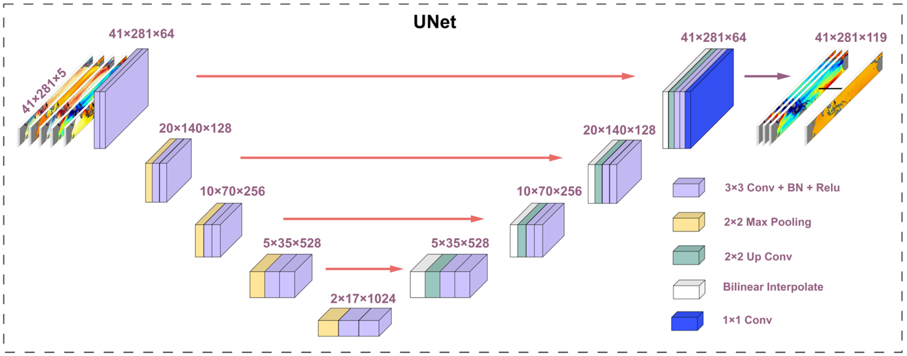
It should provide a concise and precise description of the experimental results, their interpretation, as well as the experimental conclusions that can be drawn. This study adopts UNet as the basic model architecture due to its outstanding performance in image-to-image mapping tasks. Originally designed for medical image segmentation, UNet has a structure similar to that of an auto-encoder, employing a symmetric encoder–decoder design to progressively extract and recover multi-level feature information from images [28] (Figure 2). The key innovation of UNet lies in the introduction of skip connections, where, during the decoding process, feature maps from corresponding encoder layers are concatenated with the decoder feature maps to achieve multi-scale feature fusion. The encoder (downsampling path) of UNet is used to extract multi-scale features and is primarily composed of several convolution and pooling operations that progressively reduce the spatial dimensions while enhancing feature representation. First, the input data undergoes two successive 3 × 3 convolutions, each followed by a ReLU (rectified linear unit) activation function and batch normalization to ensure stable gradient propagation and enhance nonlinear feature representation. Subsequently, the feature maps are downsampled using 2 × 2 max pooling, which reduces computational complexity and expands the receptive field. In each down-sampling stage, a set of 3 × 3 convolutions is applied immediately after max pooling, also accompanied by ReLU activation and batch normalization, to further strengthen the feature extraction capability. This downsampling process is repeated four times, gradually reducing the feature map size to 1/16 of the original input, while the number of channels increases sequentially in the order of 64, 128, 256, 512, and 1024, to accommodate the various scales of oceanic physical features. In the decoder (up-sampling path), the feature maps undergo a series of progressive expansion operations to restore spatial resolution and incorporate fine details from shallower layers. First, the feature maps are up-sampled using 2 × 2 upsampling to double the resolution. Then, these expanded features are concatenated with the corresponding encoder features that have the same spatial resolution, thereby supplementing the high-resolution information lost during downsampling. The fused features are then processed by two successive 3 × 3 convolutions, each followed by ReLU activation and batch normalization, to refine feature expression and improve recovery accuracy. This upsampling process is repeated four times, progressively restoring the spatial resolution of the feature maps, ultimately producing a high-resolution output that matches the input data. At the end of the network, the feature map output from the decoder is processed through a 1 × 1 convolution, mapping the number of channels to the number of target variables, thereby generating a 3D distribution of temperature and salinity fields corresponding to the surface fields.

3.2. Vision Transformer

In image segmentation tasks, UNet has garnered significant attention for its outstanding performance. However, due to the limited receptive field of convolution operations, this architecture has certain shortcomings in modeling global dependencies between distant pixels. This is particularly evident when dealing with complex physical field data, where capturing long-range interactions across scales can be challenging. In contrast, the Vision Transformer (ViT) fundamentally overcomes the convolutional neural network (CNN) limitation of a local-window receptive field by providing a self-attention-based paradigm for global feature modeling [29] (Figure 3).
ViT inherits the Transformer architecture originally developed for natural language processing (NLP) tasks, with its core advantage being the explicit modeling of long-distance dependencies. The Transformer computes global attention weights through the interactions between queries (Q), keys (K), and values (V), thereby overcoming the shortcomings of traditional CNNs in capturing long-range information [30]. ViT adopts a patch embedding method, dividing the input image into fixed-size patches and linearly projecting each patch into a high-dimensional feature space, while learnable positional encodings are introduced to explicitly preserve the spatial structure of the image. These patch embeddings are then fed into a stack of Transformer encoders, each consisting of a multi-head self-attention (MHSA) mechanism and a feed-forward network (FFN). The multi-head self-attention mechanism captures interdependencies within the input sequence from different feature subspaces by computing multiple attention heads in parallel, while the feed-forward network enhances feature representation through non-linear activation functions. Furthermore, the incorporation of residual connections and layer normalization ensures the stability and optimization efficiency of training deep networks [31]. Through the self-attention mechanism, ViT offers a direct modeling capability of global dependencies, providing a stronger global perspective when processing complex data.

3.3. VI-UNet

This study proposes a progressive hybrid architecture that enhances the synergistic capability of local and global features in UNet by hierarchically embedding ViT modules, achieving high-precision reconstruction of 3D ocean temperature and salinity fields (Figure 3). The architecture retains UNet’s advantage in pixel-level local feature extraction while leveraging the Transformer’s multi-head self-attention mechanism to strengthen global dependency modeling. The detailed design is as follows.
In the encoder part of the model, the standard UNet’s hierarchical design is inherited by gradually compressing the spatial resolution of feature maps through four sets of DoubleConv-Down modules. The DoubleConv module consists of two 3 × 3 convolutions, batch normalization, and ReLU activation functions; the subsequent Down module further reduces the spatial resolution of the feature maps through 2 × 2 max pooling, which suppresses high-frequency noise and expands the receptive field. Another set of DoubleConv modules is then used to increase the number of channels, thereby constructing multi-scale hierarchical representations. At the lowest level (bridge layer), the ViT module is introduced for the first time. At this stage, the feature map has the lowest resolution but a high number of channels. Specifically, a patch embedding mechanism is employed to convert the 2D feature map into a 1D token sequence, while learnable class tokens and positional encodings are added to retain spatial information. The ViT is composed of multiple Transformer Encoder Blocks, each containing LayerNorm, multi-head self-attention (MHA), and a feed-forward neural network (FeedForward Block), with residual connections to enhance stability. Finally, the tokens output by the ViT is reshaped via a modified classification head back into a 2D feature map to match the subsequent UNet decoder structure.
The decoder part also follows the UNet paradigm, using Up modules for upsampling to gradually restore spatial resolution. After each upsampling step, skip connections are used to concatenate the high-resolution features from the corresponding encoder layer with the current decoder features, thereby preserving more shallow texture information. In contrast, to incorporate additional global information modeling during the decoding process, the model sequentially embeds multi-level ViT modules after each upsampling, with parameters dynamically adapted to the current level. This approach enables the network to continuously perform long-distance dependency modeling and context fusion during the reconstruction of high-resolution features, thereby focusing on different spatial scale characteristics of the ocean scene. Finally, in the last upsampling stage, only convolution operations are retained to avoid the interference of global attention with pixel-level details, thereby better capturing subtle features such as edges and textures.

3.4. Loss Function and Experimental Configuration

The loss function is a critical parameter for evaluating and optimizing the model during training. Previous studies have shown that the Huber loss function outperforms the commonly used MSE function in subsurface temperature reconstruction tasks because it facilitates faster model convergence and reduces sensitivity to invalid values caused by topography [32]. Hence, in this study, we also adopt the Huber loss function (Equation (6)). It combines the advantages of mean squared error (MSE, Equation (4)) and mean absolute error (MAE, Equation (5)): when the error is small, it employs a squared penalty to smooth the gradient and accelerate convergence; when the error is large, it applies a linear penalty, thereby reducing sensitivity to outliers or invalid values caused by factors such as terrain.
M S E = 1 n i = 1 n ( y i f x i ) 2
M A E = 1 n i = 1 n | y i f x i |
L δ y , f x = 1 2 ( y f x ) 2 ,    | y f x | δ δ y f x 1 2 δ 2 ,    | y f x | > δ
In these expressions, L δ represents the value of the Huber loss function; y and f(x) denote the actual temperature and salinity versus the model estimates, respectively; m is the total number of data points; i indexes each data point; and δ is the hyperparameter that determines the form of the Huber loss function. Here, we set δ = 0.1, a choice based on the error scale after data normalization.
During model training, we employed an optimization process that consisted of the AdamW optimizer, the ReduceLROnPlateau learning rate scheduler, and global gradient clipping. Specifically, we first updated the model parameters using the AdamW optimizer. Compared to the traditional Adam optimizer, AdamW decouples weight decay from gradient updates, allowing for more effective control of parameter scales, stronger regularization, and a reduced risk of overfitting [33]. We set the optimizer’s initial learning rate to 1 × 10⁻³ and applied a weight decay of 1 × 10⁻⁵ to enforce L2 regularization on the model parameters. During backpropagation, we set a global gradient clipping threshold of 1.0. This means that before updating the parameters, we compute the gradient norm of all parameters, and if the norm exceeds this threshold, the gradients are proportionally scaled down to prevent gradient explosion and improve training stability [34]. Additionally, we used the ReduceLROnPlateau learning rate scheduler to dynamically adjust the learning rate based on the performance of the validation loss. When the validation loss did not improve for 10 consecutive epochs, the scheduler multiplied the current learning rate by 0.5, reducing it to help the model converge more finely in the later stages of training. To avoid the learning rate becoming too low and causing training stagnation, we set a lower bound of 1 × 10⁻⁶.

3.5. Experimental Design

We designed two sets of experiments to reconstruct 3D ocean temperature and salinity fields using the UNet and VI-UNet models (Table 1). Temperature and salinity are reconstructed independently in these experiments to better evaluate their individual impacts.

4. Results

4.1. Temperature

Temperature fields reconstructed from the VI-UNet model are in high agreement with the IAP data over the 1–6000 m water column (Figure 4), indicating that the model can accurately capture the dominant features of the oceanic thermal structure against a large-scale spatiotemporal background.
The VI-UNet model accurately reconstructs ocean temperature distributions across different depth layers, capturing essential dynamics effectively. In the surface layer (1–100 m), temperatures range broadly from 19 °C to 28 °C, reflecting strong solar radiation, air–sea interaction, and regional processes such as coastal upwelling off Peru and the warm pool in the Indian Ocean–western Pacific region influenced by ENSO conditions [35,36]. At intermediate depths (100–1000 m), the model precisely identifies a narrower temperature range (~3 °C) and key features like the frontal zone off Peru, shaped by the convergence of cold upwelling waters and the Equatorial Undercurrent [37,38]. In deeper layers (1000–3000 m), the model successfully reproduces low temperatures (<2 °C), along with localized anomalies in regions like the Arabian Sea and Bay of Bengal linked to topography and deep upwelling. At abyssal depths (3000–6000 m), temperatures stabilize around 1 °C, highlighting the model’s robustness in reconstructing subtle temperature gradients maintained by bottom currents [39]. Overall, VI-UNet demonstrates high precision and stability in temperature reconstruction across all ocean layers.
Overall, the VI-UNet model incorporating wave information not only captures fine-scale surface temperature variations but also demonstrates high accuracy in representing the overall features of temperature distribution in the intermediate and deep layers. Even in the case of sparse deep-sea data, the model can capture the temperature structure well, with only a slight underestimation in the boundary areas where abyssal data are missing.
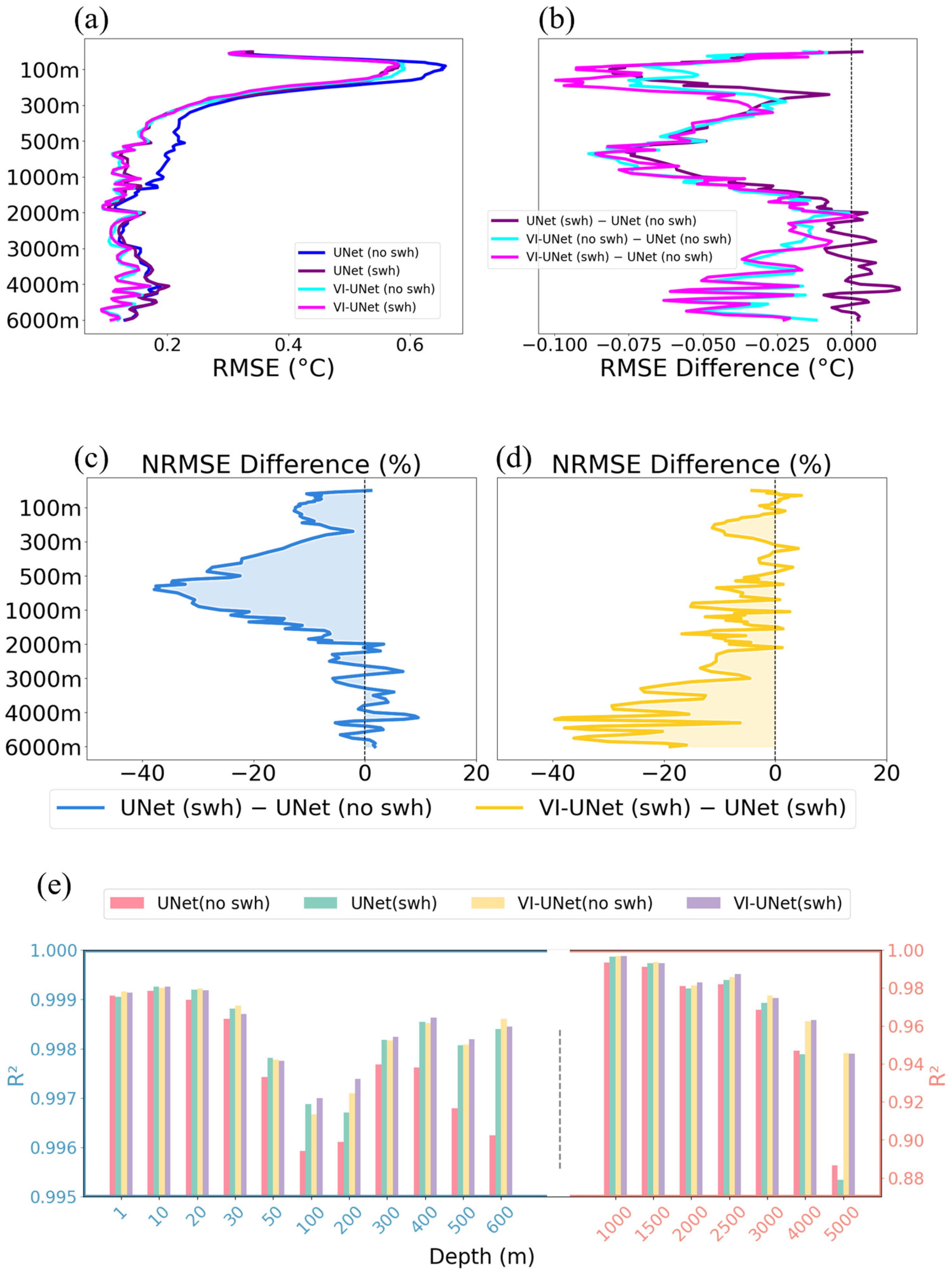
Based on the analysis of the RMSE curves in Figure 5a, the temperature reconstruction error reaches its peak, with a maximum of approximately 0.6 °C, in the 100–300 m water layer, corresponding to the thermocline. This is due to the strong vertical shear and turbulent mixing activities within this layer. In the equatorial upwelling region, the Ekman suction driven by strong wind stress curl induces vertical displacements of the thermocline, leading to dramatic changes in the temperature gradient. Combined with the superimposed effects of surface wind stress, solar radiation, and internal mixing processes, these factors result in particularly pronounced local disturbances in this layer [40].
The traditional UNet model, relying on local convolution kernels with limited receptive fields, struggles to capture the high-frequency random fluctuations associated with turbulent mixing, especially near the base of the mixed layer (around 100 m), where it shows a relatively lower R2 value (0.996). In contrast, within the 300–600 m water layer, the RMSE rapidly decreases to about 0.3 °C and stabilizes. This is primarily because the deep temperature field is mainly governed by slowly varying advection-diffusion processes; for example, the westward heat transport by the EUC results in significantly lower spatiotemporal variability in temperature compared to the upper layers [41,42].
After introducing the SWH parameter, the reconstruction errors in all depth layers above 2000 m are significantly reduced. At the 500 m layer, the NRMSE reduction is most pronounced, reaching about 40% (Figure 5c); at the critical base of the mixed layer (around 100 m), the incorporation of SWH improves the model’s R2 from 0.995 to 0.997, and the NRMSE is reduced by 20%. As an important variable representing the dynamics of the surface mixed layer, the inclusion of SWH enables the model to better capture the fluxes of surface heat and momentum that are transferred downward by surface waves and wave-driven turbulence (e.g., Langmuir turbulence and breaking waves), thereby improving the reconstruction accuracy of temperatures in the upper and mid-water layers [43,44,45]. However, in regions deeper than 2000 m, where temperature variations mainly depend on large-scale circulation and long-term water mass exchange processes, the influence of surface wave information is limited; consequently, the model with wave information shows a slight decrease in NRMSE compared to the baseline model in some cases [46].
The VI-UNet model achieves performance improvements over the traditional UNet model across the entire water column, with the NRMSE improvement increasing gradually from about 10% in the upper layers to 40% in the deep layers. The improvements in the 4000–6000 m range are particularly significant; notably, at the 5000 m layer, VI-UNet increases the R2 from an initial 0.88 to 0.94—a 7% enhancement. This marked improvement is attributed to the introduction of the attention module, which effectively integrates multi-source spatiotemporal input information to capture the key features of long-period, large-scale processes such as ocean circulation and water mass exchanges, thereby suppressing the accumulation and propagation of errors. Overall, the optimal VI-UNet model incorporating wave information achieves an R2 of approximately 0.99 in the 1–600 m layer and maintains around 0.95 even in deep water, with the RMSE remaining stable at around 0.2 °C in all layers except for the 100–300 m range. This fully validates the model’s comprehensive advantage in capturing multi-scale thermal structures and its high reconstruction accuracy across water layers dominated by different physical processes.
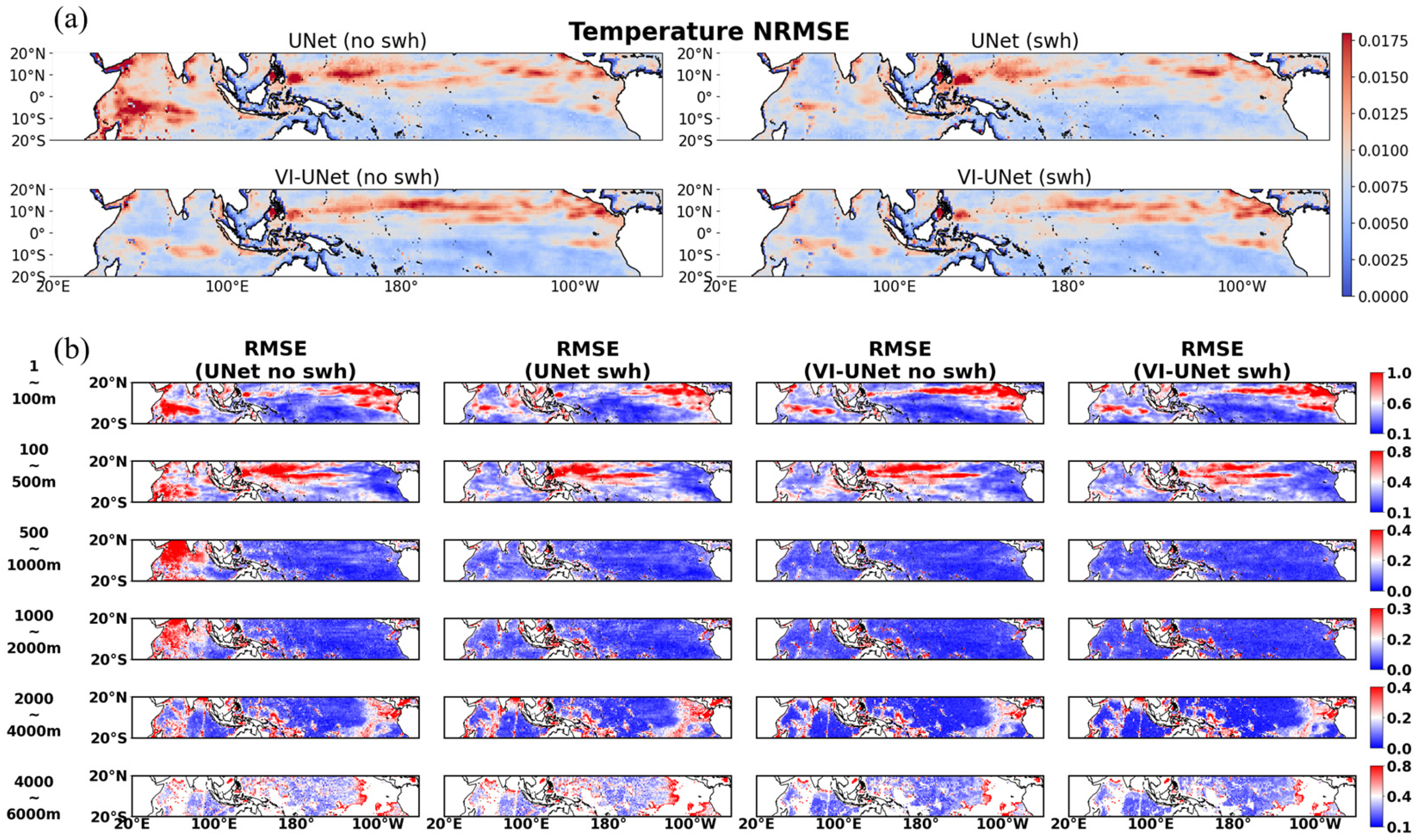
The NRMSE in most regions remains between 0.0025 and 0.0075 (Figure 6a), but in specific ocean areas, the error exhibits significant peaks. For example, in the Gulf of Aden, the Central Indian Ocean Ridge (60°E–100°E), and the equatorial western Pacific current region (10°N–20°N, 140°E–180°E), the local NRMSE even reaches 0.0175. In addition, the error shows obvious asymmetry on either side of the equator—the errors in the Northern Hemisphere are generally larger, while those in the Southern Hemisphere are smaller. This phenomenon is mainly caused by the fact that these regions are affected by persistent dynamic processes driven by strong monsoon forcing, including eddies, complex current branches, and active upwelling, which exacerbate the nonlinearity of vertical mixing and horizontal transport processes in nearshore and mid-layer waters, thereby increasing the difficulty of temperature reconstruction [47,48].
By incorporating SWH and the Vision Transformer module, the model’s performance in high-error regions has been significantly improved. Specifically, the addition of SWH reduces the NRMSE in the high-error areas of the Indian Ocean region from 0.0175 in the original model to 0.005. This improvement may stem from SWH’s ability to effectively capture the influence of surface waves on the mixed layer induced by monsoon forcing, thereby more accurately characterizing water mass mixing in wave-active nearshore regions [49]. Building on the advantages of SWH, the VI-UNet model further optimizes error control in the equatorial western Pacific region, an area that has long posed challenges for traditional convolutional neural networks due to its complex multi-scale spatiotemporal coupling (including current branches, strong eddy activities, and active upwelling).
To more intuitively reflect the improvements brought by SWH and VI-UNet across different depth layers and regions, we conducted a stratified analysis of RMSE at various depths (Figure 6b). For the surface water layer (1–100 m), the western Mexican Sea exhibits a local high error of approximately 1 °C, which corresponds to the low sea surface temperatures and distinct temperature gradients in that region, where traditional models tend to produce biases [50]. The error variation is most dramatic in the upper 500 m, ranging between 0.1 °C and 1 °C.
After incorporating SWH information, the errors in the surface and upper-intermediate layers are significantly suppressed, especially in the Central Indian Ocean region, where an error zone originally as high as about 1 °C is compressed to approximately 0.2 °C. It is worth mentioning that 2018 was an ENSO transition year and the year of the positive Indian Ocean Dipole (pIOD) event; thus, the high reconstruction errors in the 1–500 m layer may be due to the special climatic dynamical mechanisms of that year [51]. The transition of the equatorial Pacific from the residual effects of La Niña to the developing El Niño, combined with the strengthening of the positive phase of the Indian Ocean Dipole, led to complex cross-basin thermodynamic adjustments [52,53]. Such climatic adjustment is likely not well captured by the deep-learning model during the training period from January 2010 to August 2017, leading to relatively high errors.
Even in the 500–2000 m water layer, although the overall error is relatively low (most areas remain at 0–0.3 °C), the introduction of SWH still noticeably alleviates local abnormally high values, possibly because the wave effects in the upper layers transfer energy and momentum to deeper layers through vertical mixing, thereby influencing the temperature distribution in the thermocline and mid-layer waters.
Consistent with the profile analysis, for water layers below 2000 m, the role of wave information is relatively limited, whereas VI-UNet demonstrates more outstanding performance. Its multi-head attention structure is capable of deeply exploiting the slow yet critical coupling effects between deep ocean currents and surface water, effectively suppressing the layer-by-layer accumulation of errors through cross-depth dependency modeling, particularly in the 2000–6000 m depth range, thereby further reducing the already low error levels.

4.2. Salinity

Salinity more clearly reflects processes such as freshwater flux, the precipitation–evaporation balance, and circulation exchanges and is therefore crucial for understanding the seawater density structure and ocean dynamics in the region [54,55]. To further elucidate the role of SWH and the VI-UNet model in enhancing the accuracy of salinity reconstruction, this section employs a modeling approach similar to that used for temperature reconstruction.
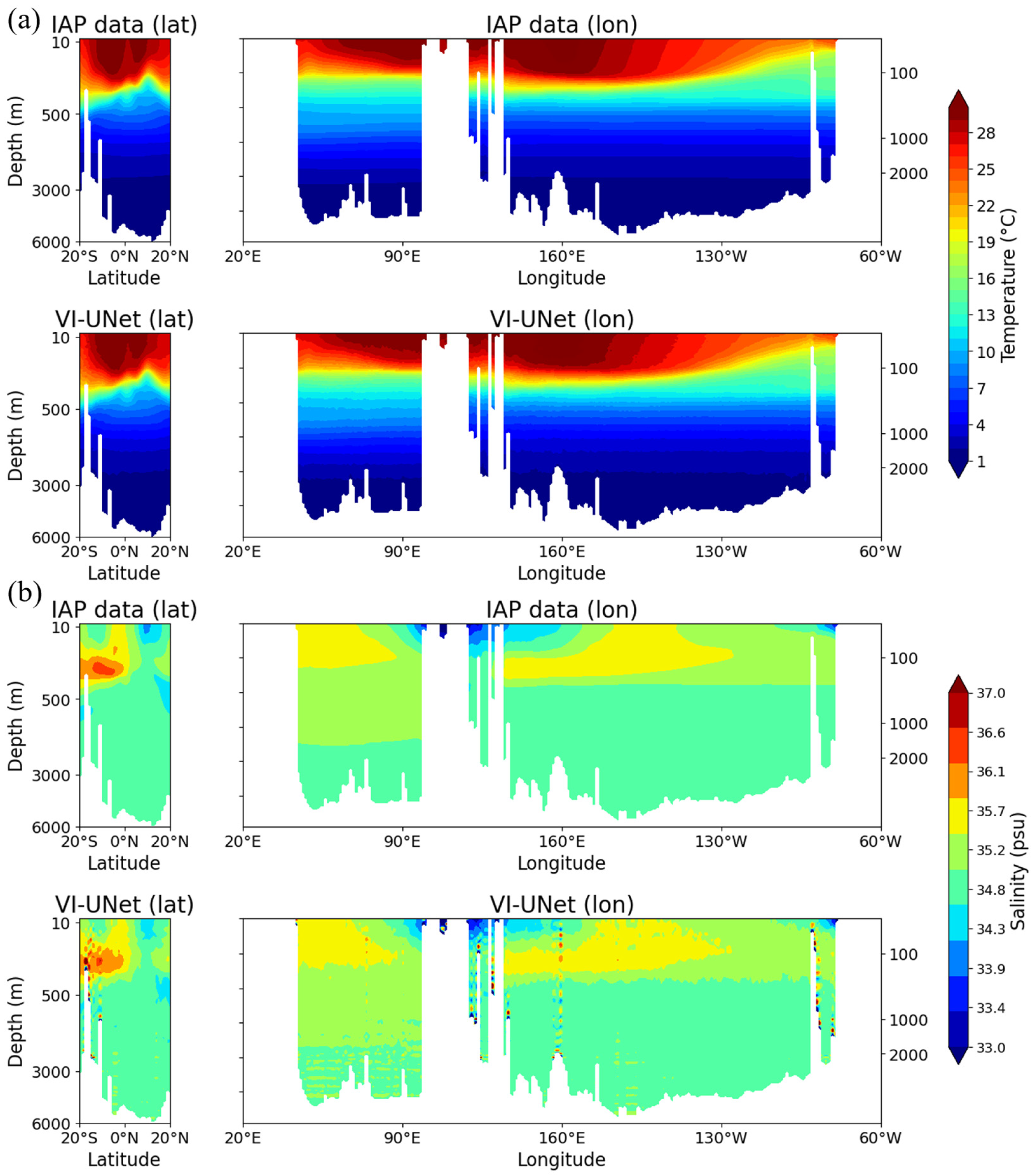
Based on a comparative analysis of the 2018 full-depth (1–6000 m) IAP data and the VI-UNet model salinity reconstruction results (Figure 7), the salinity distribution in the study area shows a high degree of vertical structural consistency between the model and the observed data, while also revealing the complex regulatory mechanisms of ocean dynamics on salinity variations within each water layer.
The VI-UNet model effectively reconstructs salinity distributions across different ocean layers, accurately capturing key hydrological features influenced by ocean dynamics. In the surface and subsurface layers (1–1000 m), the model identifies high-salinity regions accurately, including the eastern Pacific cold tongue, Gulf Stream region, and Arabian Sea, reflecting the combined effects of evaporation, precipitation, and ocean currents [56,57,58]. At mid-water depths (1000–3000 m), the model successfully captures the more homogeneous salinity distribution driven by deep circulation and accurately represents the southward diffusion of the low-salinity North Pacific Intermediate Water (NPIW) [59,60]. In the abyssal layer (3000–6000 m), despite sparse observational data, the model robustly reconstructs weak salinity variations influenced by slow-moving water masses such as Antarctic Bottom Water (AABW) and North Atlantic Deep Water (NADW) [61]. Overall, the integration of physical variables and wave information in the VI-UNet model ensures precise and stable salinity reconstruction across diverse ocean depths.
Comparative analysis of salinity reconstruction results based on observational data indicates that the vertical distribution error of salinity in the study area exhibits significant depth-dependent characteristics (Figure 8). In the surface and subsurface layers (1–1000 m), the reconstruction error for salinity is relatively high; for example, the 1 m layer shows an RMSE of about 0.5–0.75 psu with an R2 of 0.992—the lowest value observed across the entire water column. However, as depth increases, the model performance gradually improves; below 300 m, the R2 stabilizes above 0.998, and the RMSE drops significantly from the peak values seen at the surface. In particular, in the deep layers below 2000 m, the VI-UNet model that incorporates SWH information can reduce the RMSE to below 0.005 psu.
The introduction of SWH shows an obvious vertical demarcation effect on the improvement of salinity reconstruction—in the upper 1–1000 m, including SWH significantly enhances the model’s ability to reconstruct salinity. For instance, near the depths of 1–100 m and around 1000 m, the RMSE is reduced by up to 0.25 psu and the NRMSE decreases by about 20%. This improvement is consistent with the upward optimization trend observed in temperature reconstruction, confirming that the representation of surface dynamic processes by wave information plays a crucial role in salinity structure reconstruction.
However, a negative impact of SWH is observed in deep salinity reconstruction (below 1000 m). This may be because the evolution of deep salinity is primarily controlled by long-period processes—such as inter-basin water mass exchanges (e.g., the slow intrusion of Antarctic Bottom Water) and meridional overturning circulation—which are minimally sensitive to surface wave forcing [62]. In this context, SWH might introduce noise signals that do not match the physical mechanisms governing the deep layer, thereby interfering with the model’s reconstruction of a steady-state salinity field. Nevertheless, the significant advantages of SWH in upper layer salinity reconstruction still lead to an overall NRMSE improvement of 20–30% for the 1–1000 m range, underscoring the necessity of multi-source data fusion in depicting surface dynamic processes.
In contrast to the localized improvements achieved by SWH, the VI-UNet model that incorporates the Vi-Transformer attention mechanism provides a more comprehensive and significant optimization for salinity reconstruction. By dynamically modeling the covariant relationships of salinity across different depths and regions, the model achieves a systematic error reduction throughout the entire water column, with the average NRMSE decreasing by 50% and the RMSE reduced by 0.25–1.0 psu. At a depth of 10 m, the R2 improves from 0.9994 to 0.999, and the RMSE is reduced by approximately 0.75 psu; in the intermediate layer (100–2000 m), the NRMSE continuously decreases by 50%; and in the abyssal layer (3000–6000 m), the Vi-Transformer—by exploiting the long-range spatial correlations of water mass properties—achieves an NRMSE improvement of up to 100%.
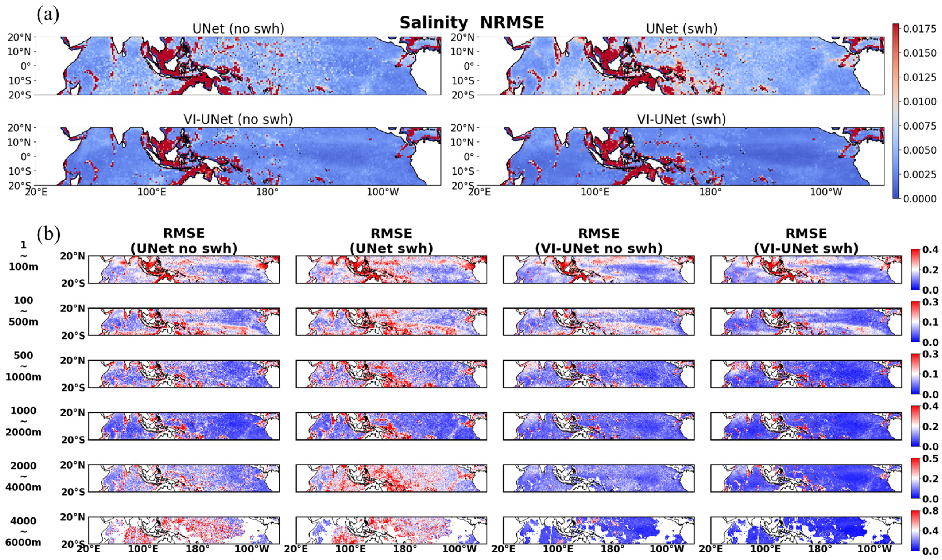
The reconstructed salinity fields exhibit higher errors in nearshore and island-dense regions (e.g., Figure 9a, the Southeast Asian archipelago and the Indian Ocean coastline). Areas with numerous islands, such as the Indonesian Archipelago, the Philippine Islands, and the Maldives region, are influenced by a combination of processes, including rainfall, estuarine freshwater input, tides, and upwelling [63,64], leading to rapid salinity changes over short distances. Additionally, the intricate shorelines, significant topographic and depth variations, and complex pathways of seawater exchange make these areas far more challenging to model than open oceans. Even with relatively comprehensive satellite remote sensing or other observational methods, these micro-scale or semi-enclosed regions often suffer from observational blind spots or insufficient data assimilation, resulting in persistently higher reconstruction errors in island-dense zones.
A comparative analysis of the salinity reconstruction error distribution across the study area’s water masses reveals significant horizontal and vertical heterogeneity in error accuracy (Figure 9b). Horizontally, the salinity RMSE in island-dense regions such as the Indonesian Archipelago is notably higher than that in the open ocean, and these localized high-error zones significantly elevate the overall error of the vertical profile (Figure 8a); meanwhile, the RMSE in the open ocean consistently remains below 0.2 psu. Vertically, the improvement characteristics vary markedly among different water layers: in the surface to subsurface layer (0–1000 m), the SWH parameter characterizes wind–wave mixing processes and reduces the RMSE by approximately 20% in the open ocean of the Indian Ocean and western Pacific.
The high error “patches” in salinity reconstruction may, to some extent, be attributed to the limitations of satellite salinity data itself. Although the spatial resolution has been unified to a 1° × 1° grid during the data preprocessing stage, the spatial variability of seawater salinity inherently exhibits higher randomness and discontinuity compared to temperature fields. Satellite salinity observations are easily affected by multiple factors, such as radio frequency interference, changes in sea surface roughness, and complex oceanic dynamic processes, all of which inevitably introduce “noise” into the data. Particularly in regions with complex topography, such as the Indonesian archipelago, the small-scale salinity gradients generated by complex oceanic dynamic processes (such as intense tidal mixing, monsoon-driven coastal upwelling, and freshwater input from rivers) often exceed the spatial resolution of satellites, which further exacerbates the uncertainty of the “ground truth.” These inherent limitations of the underlying data cannot be fully eliminated in the reconstruction process.
Although the salinity data itself has inherent limitations, VI-UNet has still largely overcome these data noise and spatial heterogeneity issues. In contrast, the VI-UNet model demonstrates optimization across the entire water column—it not only continuously improves the salinity field in the open ocean below 100 m but also reduces the error peak from 0.5 psu to 0.3 psu in regions surrounding the Indonesian Archipelago where the traditional UNet exhibits pronounced errors. With increasing depth, the model’s advantages become even more apparent—in the mid-water layer (2000–4000 m), the attention mechanism successfully smooths out the high-error “patches” left by the UNet, driving the overall RMSE down to below 0.1 psu. Notably, in the abyssal layer (4000–6000 m) where observational data are scarce, a breakthrough is achieved as the error sharply decreases from 0.8 psu in the UNet to 0.1 psu.
It is also noteworthy that compared to the negative impact observed in the deep water layer when introducing the SWH parameter into the UNet (Figure 8d), the VI-UNet model with the SWH parameter shows an ability to optimize the entire water column in the open ocean. This may be attributed to its attention mechanism, which indirectly establishes a potential linkage between surface dynamic processes and deep circulation, thereby achieving the optimal overall performance in 3D salinity field reconstruction.

5. Discussion

5.1. Profiles at Longitudinal and Zonal Sections

To analyze the spatial heterogeneity of 3D ocean dynamics in depth, this study focuses on two key sections—the 180° longitude section (traversing the central Pacific depicted in Figure 1) and the 0° latitude section (the equatorial cross-section)—to reveal subtle changes in water mass structure. The meridional section extends from the eastern Pacific’s Peru cold current influence zone to the core area of the western Pacific warm pool, precisely covering the key channel for ENSO (El Niño–Southern Oscillation) signal transmission [65]. Meanwhile, the zonal section crosses the convergence zone of the EUC and the south equatorial current (SEC), where there is not only a pronounced equatorial upwelling but also seasonal modulation by the tropical convergence zone (ITCZ) [66].
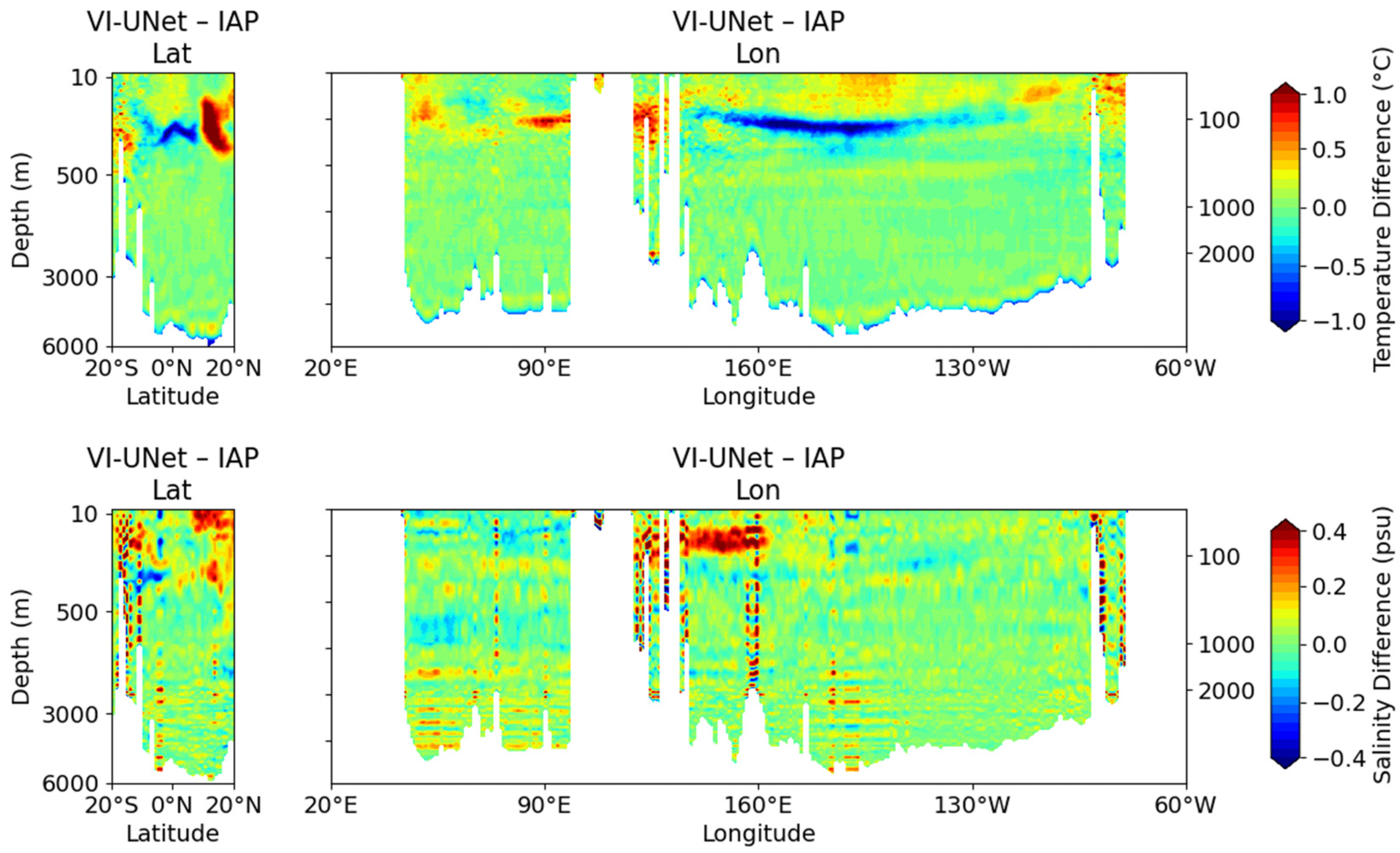
Overall, the VI-UNet model exhibits excellent performance in reconstructing temperature and salinity profiles (Figure 10), capturing numerous subtle gradients and structural features in both sections. For the temperature reconstruction, the model successfully reproduces the unique shallow mixed layer structure of the eastern Pacific (130°W–70°W), where the mixed layer depth is less than 50 m—considerably shallower than that observed at similar latitudes in the western Pacific, a feature closely related to the strong trade wind–driven Ekman suction in that area [67]. Above 500 m, distinct temperature gradients develop in different regions, while deep water temperatures remain stably below 8 °C. Additionally, the zonal section indicates that the mixed layer near approximately 5°N is the shallowest, and that water temperatures around 0° are 1–2 °C lower than those in the surrounding areas—a phenomenon that may be related to the role of local circulation systems in regulating heat transport and distribution [67]. Through difference analysis of the IAP data and the reconstruction results (see Figure 11), it is evident that the temperature reconstruction errors are primarily concentrated within the thermocline between approximately 100 m and 500 m, where the ocean’s thermal structure undergoes rapid change. Spatially, these errors exhibit pronounced heterogeneity: in the equatorial core region (around 0°N), the model systematically underestimates temperature by more than 1 °C, whereas in the northern equatorial band (0–20°N) it overestimates by roughly 1 °C. Such biases are particularly marked over complex bathymetric features. By contrast, in the deep ocean (>500 m) and in the surface mixed layer (<50 m), where temperature gradients are more gradual, reconstruction errors generally remain within 0–0.2 °C, demonstrating high accuracy and stability.
Regarding the salinity reconstruction, a low-salinity area corresponding to the low-temperature region appears within the upper 500 m of the eastern Pacific. In the zonal section, within the 0–20°S range of the Southern Hemisphere at around 300 m depth, a significant high-salinity core (>35.7 psu) is formed, extending horizontally up to 2000 km and vertically spanning 200 to 500 m. The formation of this high-salinity core is mainly attributed to the subduction of high-salinity surface water in the Ekman convergence zone, which is further enhanced by the meridional advection superposition with subsurface South Pacific tropical water (SPTW) [68]. Compared to the temperature reconstruction, the salinity field differences exhibit far more pronounced spatial oscillations (Figure 11). In the salinity profiles, localized “speckle” noise likely originates from data instability and from boundary effects at the land–sea interface. A detailed quantitative analysis reveals systematic positive biases of 0.3–0.4 psu in the upper 10 m layer near 20°N, as well as additional high-bias patches in the 150–160°E sector. These deviations may stem from the rapid response of surface salinity to atmospheric forcing, which generates high-frequency fluctuations in both time and space. Moreover, the interaction of mesoscale eddies with frontal structures intensifies local salinity gradients, producing anomalous signals in select regions. Despite these localized biases, the reconstruction model successfully captures the principal structural features of the salinity field, with reconstructed differences remaining below 0.2 psu across the vast majority of the domain. Overall, the reconstruction effectively captures the main features.
In addition, we have also observed that salinity reconstruction is influenced by sharp topography in different latitude and longitude profiles. The oceanic dynamic processes of sharp topography often exhibit high complexity and discontinuity, leading to intense vertical mixing and turbulence in these areas, which, in turn, causes significant variations in local salinity distribution. Furthermore, sharp topography often acts as a physical barrier for water mass boundaries, forming interfaces between different water mass characteristics. This contrast effect between water masses may be a major cause of speckle noise in salinity reconstruction.

5.2. Seasonal Variations

In 2018, the equatorial Pacific was at a critical transition stage from a weak La Niña to an ENSO-neutral state, during which the sub-surface thermal structure exhibited a distinct “warm west, cool east” spatial pattern [69]. Research indicates that although the seasonal variation of SST in the equatorial region is generally less than 3 °C, the seasonal oscillations of the wind field and the Ekman suction effect drive particularly active dynamics in the thermocline of the eastern Pacific upwelling region, resulting in significant seasonal fluctuations of 4 to 5 °C in heat content within the 100 to 300 m depth range [70].
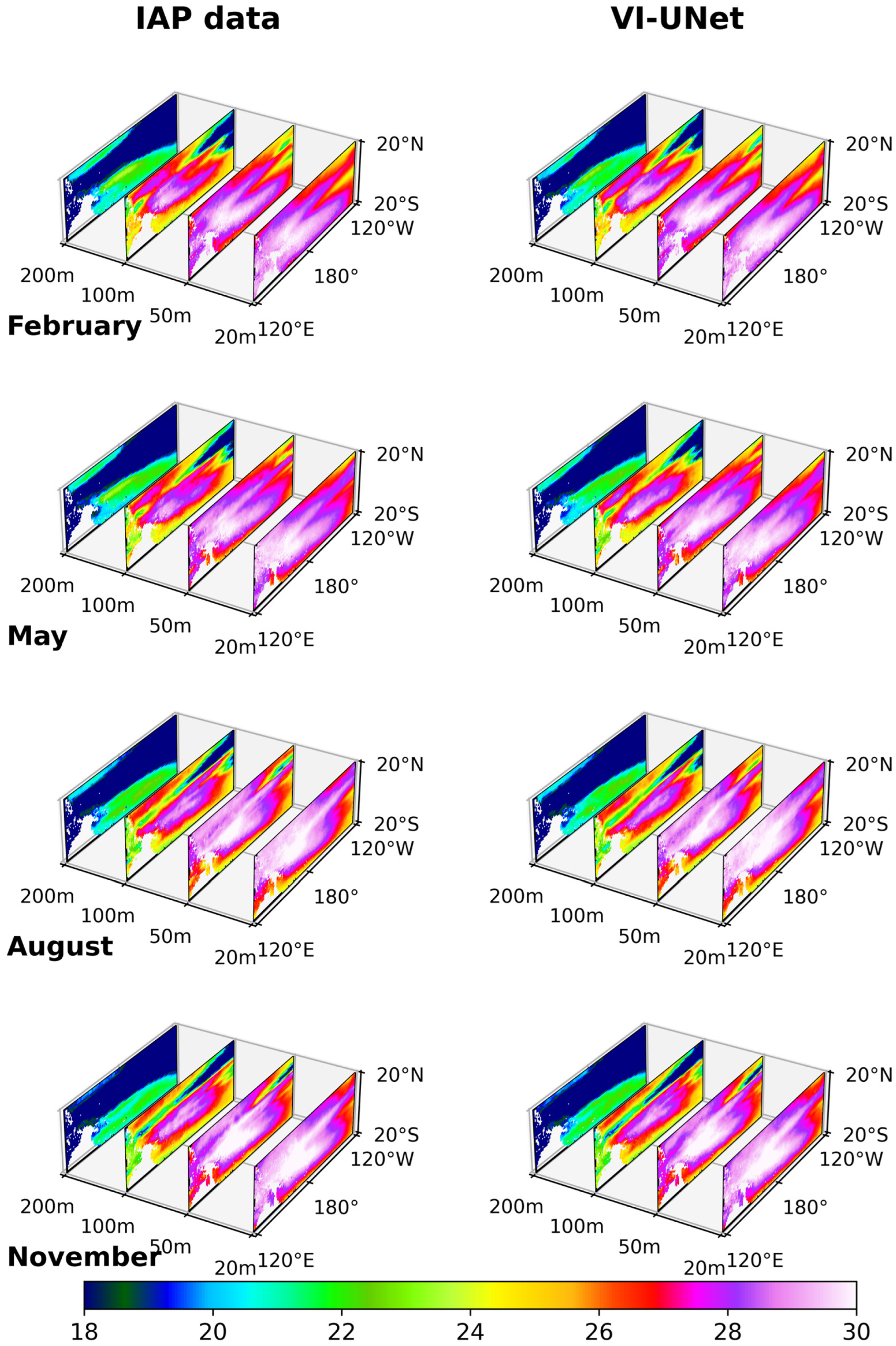
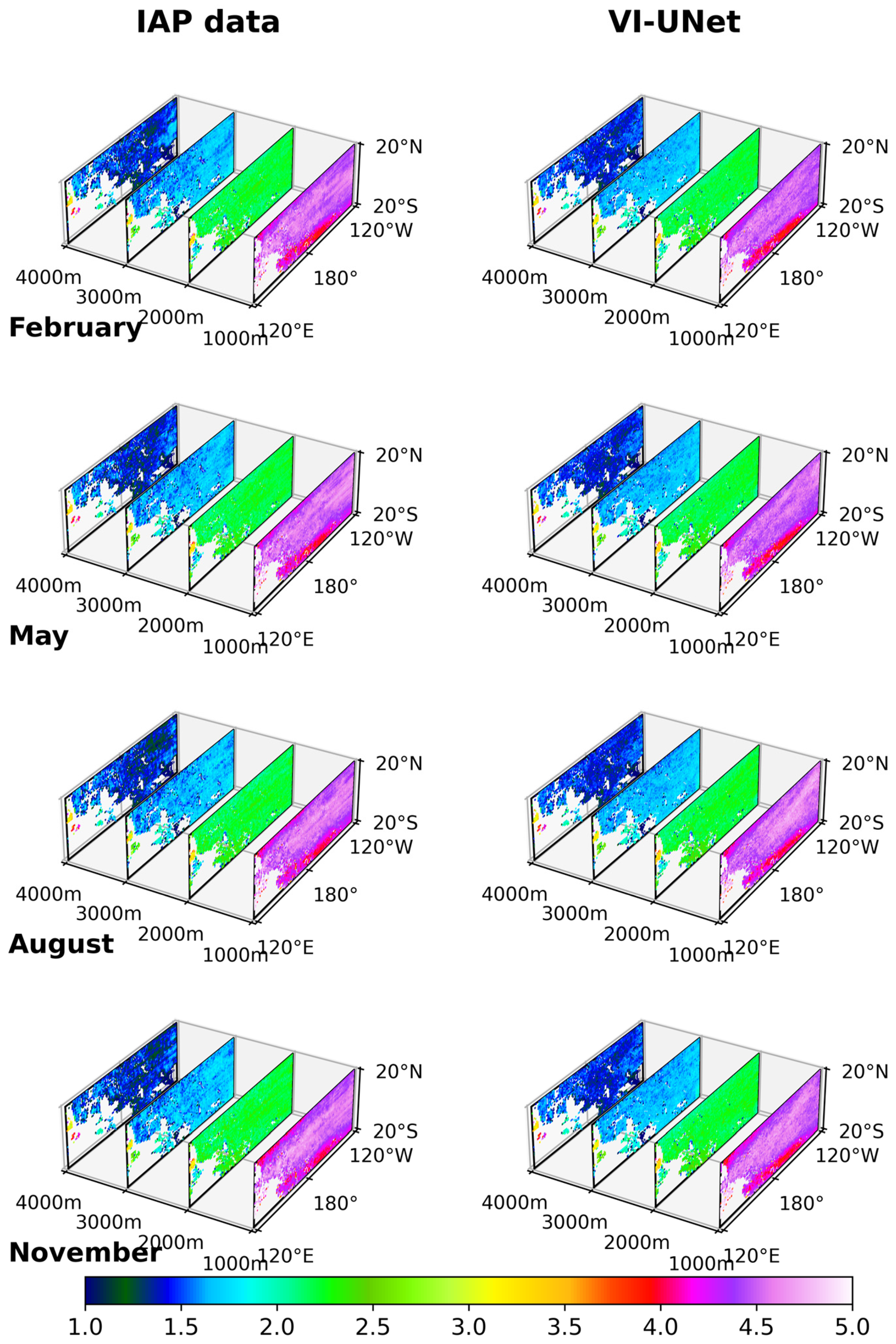
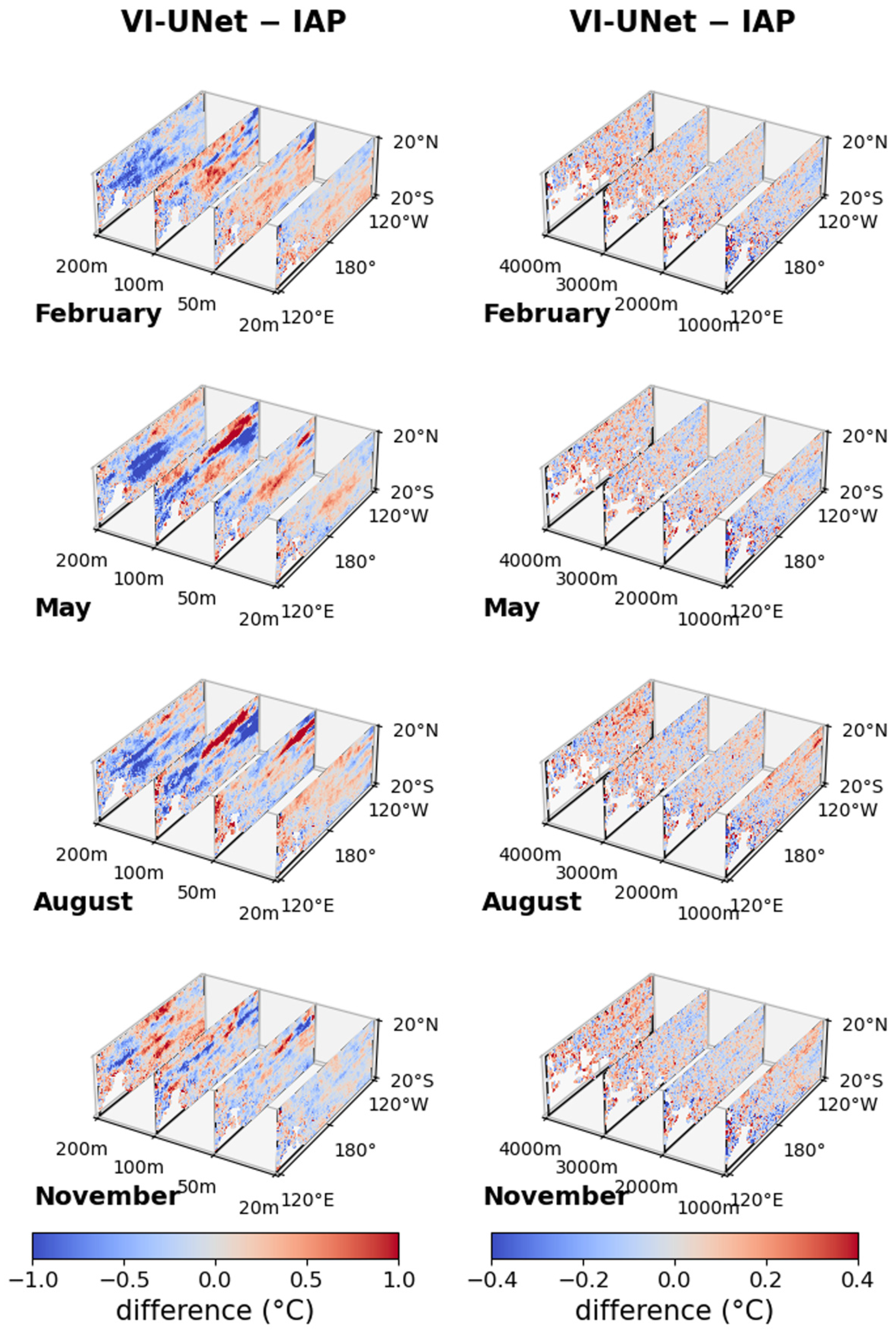
Based on this climatic background, we used the VI-UNet model with SWH to conduct a detailed comparison of the reconstructed temperature fields with IAP data across various depth layers for February, May, August, and November 2018 (Figure 12 and Figure 13). The results show that the VI-UNet model exhibits excellent performance in capturing seasonal variability and the vertical temperature structure, with the reconstruction results at all depth layers being highly consistent with the observations.
Although the study area spans both sides of the equator and the seasonal variations of the upper and deep water temperatures do not differ significantly, there are still notable local variations: the eastern Pacific cold tongue displays a typical seasonal migration characteristic—in February and May, the cold tongue extends broadly with its western edge reaching approximately 160°W; whereas in August and November, it contracts noticeably to the east, which is closely related to the seasonal intensification of the EUC [71,72].
At the same time, the equatorial region in the central Pacific consistently maintains the highest temperatures, corresponding to the warm pool area in the western Pacific—this area shows a gradually shrinking trend from 20 m to 100 m, while the 100 to 200 m layer generally constitutes a transitional layer of rapid temperature decline, and below 200 m, the temperatures are relatively uniform with markedly reduced thermal differences.
Additionally, although the model slightly underestimates the temperatures in the western Pacific warm pool at the 100 m layer for each month, the overall trend clearly reflects that the surface high-temperature zone can exceed 30 °C in every month, gradually shrinking with depth, and by 200 m, it is noticeably weakened to below 25 °C; in deeper layers, the temperature gradient becomes relatively gentle, showing only subtle seasonal differences between the deep water and intermediate layers—from about 4 °C at 1000 m to around 2 °C at 2000 m, and to approximately 1 °C at 3000–4000 m. In our difference analysis of the reconstructed temperature field, the 20–200 m mid-upper layer exhibits a relatively uniform error distribution, whereas the deeper strata below 200 m display pronounced spatial oscillations (Figure 14). This contrast likely stems from the coarser resolution and sparse sampling of the original observations in the deep ocean. Moreover, the weak seasonality and thermally stable structure of deep waters result in minimal month-to-month variation in reconstruction error. By contrast, mid-upper waters (20–200 m) respond more directly to atmospheric forcing and therefore exhibit strong seasonal variability, with error fluctuations peaking in May and August. At 100 m depth, the error field assumes a clear bipolar pattern: systematic underestimation (negative bias) in the western Pacific warm pool and systematic overestimation (positive bias) in the eastern Pacific cold tongue, both exceeding 1 °C in magnitude. Examining the temporal evolution, February errors are relatively homogeneous: the 20 m and 50 m layers show a consistent positive bias of 0.3–0.5 °C, while the 100 m layer begins to manifest more complex regions of over- and underestimation. By May, error maxima concentrate around the 100 m layer, reinforcing the bipolar structure between the warm pool and cold tongue. This pattern persists into August, albeit with diminishing intensity, and further attenuates by November. Nevertheless, even in late autumn, the 100 m and 200 m layers maintain significantly larger errors than the shallower 20 m and 50 m layers.
In brief, the VI-UNet model with SWH demonstrates an extremely detailed capability in capturing oceanic features across different seasons and depth layers, fully showcasing its precise ability to reproduce 3D ocean dynamics.

5.3. Evaluation During Climate Phenomena

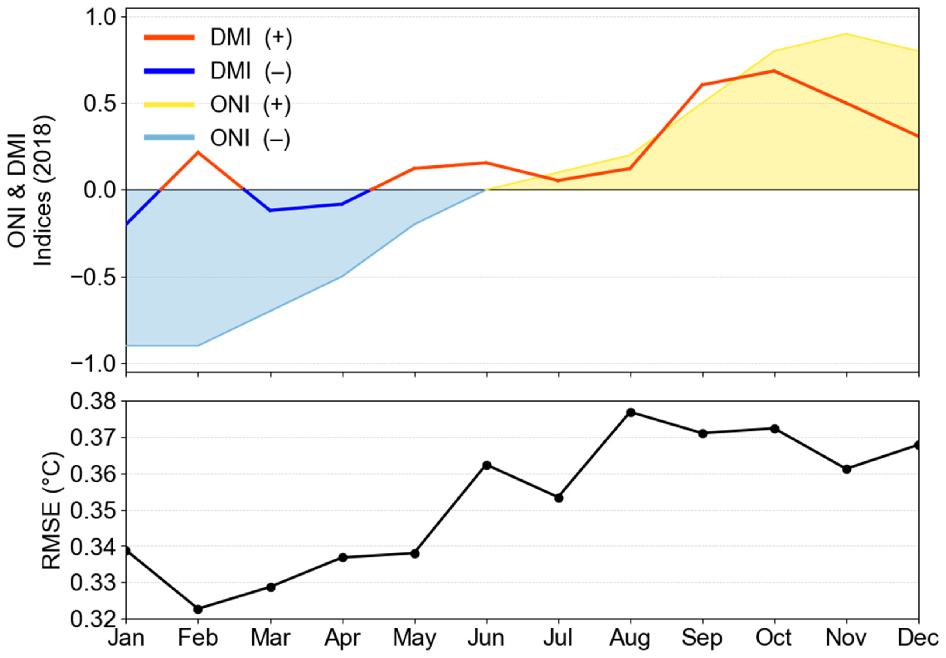
In 2018, the tropical oceans were jointly modulated by a weakening La Niña and a rapidly developing positive Indian Ocean dipole (IOD). The equatorial central-eastern Pacific retained residual La Niña conditions from January to March (Niño-3.4 ≤ −0.5 °C) before returning to neutral in April–May. Meanwhile, the IOD peaked in September–October, exhibiting the classic “cool-west/warm-east” pattern. The combined ENSO–IOD signals reshaped the Walker circulation, the Indonesian throughflow, and equatorial upwelling, imposing marked seasonal modulation on the region’s baroclinic structure and heat transport. This modulation is reflected in the temperature-reconstruction performance: during the quiescent phase (January–May), circulation is gentle and mixed-layer depth changes are limited, keeping the RMSE at 0.32–0.34 °C; during the dynamic phase (June–December), the intensified IOD, together with eastward-propagating La Niña anomalies, steepens the thermocline and enhances cross-basin heat redistribution, raising the RMSE to 0.35–0.38 °C (Figure 15). Although the error increase is only ~0.04 °C, it indicates a heavier burden on the model in capturing the intensified monsoon–eddy coupling, while still demonstrating its robustness under complex background conditions.

5.4. Multi-Scale Self-Attention and Wave Physical Constraints

Compared with traditional machine learning models, UNet employs a symmetric “encoder–decoder + skip-connection” architecture to extract spatial features at multiple scales in a hierarchical fashion. Building on this foundation, VI-UNet innovatively integrates a multi-scale Vision Transformer module: its self-attention mechanism effectively captures long-range dependencies both across depth levels and over distant spatial regions. This design is especially well-suited to the data-sparse deep-ocean environment, compensating for the inability of conventional convolutional networks to cover global contextual information and rendering VI-UNet much more sensitive to subtle structures in weak-gradient deep layers. This finding is consistent with the recent PGTransNet study based on a pure Transformer backbone, which demonstrated that self-attention significantly enhances the resolution of low-frequency, long-range coupled signals [73].
Our second improvement is to introduce SWH as a critical physical constraint within the network. Surface waves can enhance vertical mixing via processes like wave breaking and Langmuir turbulence, markedly deepening the mixed layer and strengthening vertical heat-salt exchange [43,44,45]. Traditional temperature–salinity reconstruction methods typically neglect wave–current interactions, leading to a systematic underestimation of thermocline intensity. By incorporating SWH into the model, the network learns during training to capture the modulation of heat-salt profiles by wave–flow–turbulence coupling, thereby further improving reconstruction accuracy.
Moreover, deep learning demonstrates remarkable advantages in the fusion of multi-source in situ and remotely sensed observations. Satellite remote sensing provides broad-coverage, high spatiotemporal resolution surface fields that complement Argo, CTD and other profile measurements, greatly enhancing information completeness. This study relies solely on observational and remote sensing data, thereby avoiding any systematic biases introduced by numerical models. Previous work has shown that a feed-forward neural network (FFNN) fusing satellite and profile data can successfully reconstruct a high-resolution salinity field from 0 to 2000 m over the period 1993–2018, validating the efficacy of multi-source data fusion in suppressing deep-ocean reconstruction errors [74]. Our VI-UNet model further refines this fusion strategy—by combining self-attention with hierarchical feature extraction, it maintains high surface accuracy while significantly improving reconstruction quality in the mid-to-deep layers.

6. Conclusions

In oceanographic research, accurately estimating subsurface temperature and salinity structures is crucial for a deeper understanding of ocean dynamics and climate change. By integrating multi-source satellite remote sensing data with CTD, Argo, Bottle, and other in situ observations, this study evaluated the impact of incorporating SWH information into deep-learning models UNet and VI-UNet on the reconstruction of 3D temperature and salinity.
Comprehensive analyses indicate that in the upper ocean layer (approximately 1–1000 m) influenced by the combined effects of surface waves and wave-driven processes, incorporating SWH can markedly enhance the model’s ability to capture wave-related mixed layer dynamics, thereby effectively reducing reconstruction errors for temperature and salinity. In particular, in the thermocline region (100–300 m) and in tropical regions with active wind–waves (e.g., the Indian Ocean and the equatorial western Pacific current areas), adding SWH information reduces the NRMSE of temperature by up to 40%, while the NRMSE of salinity is improved by 20–30%. Furthermore, in the deep ocean, the VI-UNet model—integrating a multi-scale Vision Transformer module—demonstrates even more significant advantages; when wave information is incorporated, the NRMSE of temperature and salinity improves by 40% and 100%, respectively.
These results fully demonstrate the key role of SWH in capturing the dynamics of the ocean mixed layer and enhancing the 3D reconstruction accuracy of deep ocean temperature and salinity fields. Furthermore, compared to the UNet model, the VI-UNet model exhibits superior reconstruction performance in multi-scale ocean environments.
Despite the overall high accuracy of the models, reconstruction errors remain relatively elevated in regions with frequent monsoons, typhoons, and eddies (e.g., nearshore Indian Ocean and western equatorial current zones), as well as in island-dense areas. On the one hand, with the increasing availability of diverse ocean remote sensing observations (e.g., wave fields, sea ice, ocean vorticity) and more types of buoy data [75], future efforts could explore the incorporation of more comprehensive physical feature factors to enhance model generalization. On the other hand, combining attention mechanisms with more refined dynamic constraints (e.g., coupled ocean–atmosphere models) holds promise for improving reconstruction performance in extreme conditions or data-sparse regions. Additionally, targeted corrections for high-latitude and island-dense regions, as well as detailed modeling of deep-water layers, should be prioritized in future research.

Author Contributions

Conceptualization, D.L.Y. and P.W.; data curation, X.Y.; formal analysis, X.Y.; funding acquisition, P.W.; investigation, X.Y.; project administration, P.W.; resources, P.W.; supervision, P.W.; visualization, X.Y.; writing—original draft, X.Y.; and writing—review and editing, D.L.Y. and P.W. All authors have read and agreed to the published version of the manuscript.

Funding

This research was funded by the National Key Research and Development Program of China (grant nos. 2024YFC3013200 and 2023YFC3008200), the Natural Science Foundation of the Guangdong Province (grant no. 2022A1515110914), and the National Natural Science Foundation of China (NSFC) (grant nos. 42306011 and 42206017).

Data Availability Statement

Surface temperature (SST) data are obtained from the National Oceanic and Atmospheric Administration (NOAA) (http://apdrc.soest.hawaii.edu/data/data.php, accessed on 10 October 2024). The sea surface salinity (SSS) dataset is provided by the European Space Agency (ESA) Climate Change Initiative (CCI) project (https://climate.esa.int/en/data/#/dashboard, accessed on 13 October 2024). Sea surface height (SSH) and significant wave height (SWH) data are obtained from the Archiving, Validation, and Interpretation of Satellite Oceanographic datasets (AVISO) (http://www.aviso.altimetry.fr, accessed on 13 October 2024). The sea surface wind (SSW) data is derived from the Cross-Calibrated Multi-Platform (CCMP) ocean surface wind vector analysis product (https://rda.ucar.edu/datasets/ds745.1/, accessed on 20 October 2024). The full-depth temperature and salinity are sourced from a global gridded ocean temperature and salinity product provided by the Institute of Atmospheric Physics (IAP), Chinese Academy of Sciences (https://argo.ucsd.edu/data/argo-data-products/, accessed on 5 November 2024).

Acknowledgments

We would like to express our sincere gratitude to the three anonymous reviewers for their valuable comments and suggestions.

Conflicts of Interest

The authors declare that they have no known competing financial interests or personal relationships that could have appeared to influence the work reported in this paper.

References

  1. Wang, B.; Hua, L.; Mei, H.; Wu, X.; Kang, Y.; Zhao, N. Impact of Climate Change on the Dynamic Processes of Marine Environment and Feedback Mechanisms: An Overview. Arch. Comput. Methods Eng. 2024, 31, 3377–3408. [Google Scholar] [CrossRef]
  2. Ren, J.; Wang, C.; Sun, L.; Huang, B.; Zhang, D.; Mu, J.; Wu, J. Prediction of Sea Surface Temperature Using U-Net Based Model. Remote Sens. 2024, 16, 1205. [Google Scholar] [CrossRef]
  3. Webster, P.J. The Role of Hydrological Processes in Ocean-Atmosphere Interactions. Rev. Geophys. 1994, 32, 427–476. [Google Scholar] [CrossRef]
  4. Chen, Z.; Zhou, T.; Zhang, L.; Chen, X.; Zhang, W.; Jiang, J. Global Land Monsoon Precipitation Changes in CMIP6 Projections. Geophys. Res. Lett. 2020, 47, e2019GL086902. [Google Scholar] [CrossRef]
  5. Planton, Y.Y.; Vialard, J.; Guilyardi, E.; Lengaigne, M.; McPhaden, M.J. The Asymmetric Influence of Ocean Heat Content on ENSO Predictability in the CNRM-CM5 Coupled General Circulation Model. J. Clim. 2021, 34, 5775–5793. [Google Scholar] [CrossRef]
  6. Roemmich, D.; Gilson, J.; Wijesekera, H.; Wong, A.P.; Wijffels, S.E.; Riser, S.C.; Pouliquen, S.; Hosoda, S.; Poffa, N.; Park, H.M.; et al. Argo Data 1999–2019: Two Million Temperature-Salinity Profiles and Subsurface Velocity Observations from a Global Array of Profiling Floats. Front. Mar. Sci. 2020, 7, 700. [Google Scholar] [CrossRef]
  7. Dickey, T.; Lewis, M.; Chang, G. Optical Oceanography: Recent Advances and Future Directions Using Global Remote Sensing and In Situ Observations. Rev. Geophys. 2006, 44, RG000148. [Google Scholar] [CrossRef]
  8. Li, D.; Wang, P. Global Wavenumber Spectra of Sea Surface Salinity in the Mesoscale Range Using Satellite Observations. Remote Sens. 2024, 16, 1753. [Google Scholar] [CrossRef]
  9. Dubovik, O.; Schuster, G.L.; Xu, F.; Hu, Y.; Bösch, H.; Landgraf, J.; Li, Z. Grand Challenges in Satellite Remote Sensing. Front. Remote Sens. 2021, 2, 619818. [Google Scholar] [CrossRef]
  10. Meng, L.; Yan, X. Remote Sensing for Subsurface and Deeper Oceans: An Overview and a Future Outlook. IEEE Geosci. Remote Sens. Mag. 2022, 10, 72–92. [Google Scholar] [CrossRef]
  11. Schuster, G.T.; Chen, Y.; Feng, S. Review of Physics-Informed Machine-Learning Inversion of Geophysical Data. Geophysics 2024, 89, 1ND–V667. [Google Scholar] [CrossRef]
  12. Weglein, A.B.; Zhang, H.; Ramírez, A.C.; Liu, F.; Lira, J.E. Clarifying the Underlying and Fundamental Meaning of the Approximate Linear Inversion of Seismic Data. Geophysics 2009, 74, 1ND–Z107. [Google Scholar] [CrossRef]
  13. Hu, L.Y.; Chugunova, T. Multiple-Point Geostatistics for Modeling Subsurface Heterogeneity: A Comprehensive Review. Water Resour. Res. 2008, 44, W11410. [Google Scholar] [CrossRef]
  14. Haines, K. A Direct Method for Assimilating Sea Surface Height Data into Ocean Models with Adjustments to the Deep Circulation. J. Phys. Oceanogr. 1991, 21, 843–868. [Google Scholar] [CrossRef]
  15. Wong, M.S.; Jin, X.; Liu, Z.; Nichol, J.E.; Ye, S.; Jiang, P.; Chan, P.W. Geostationary Satellite Observation of Precipitable Water Vapor Using an Empirical Orthogonal Function (EOF) Based Reconstruction Technique over Eastern China. Remote Sens. 2015, 7, 5879–5900. [Google Scholar] [CrossRef]
  16. Cassou, C.; Minvielle, M.; Terray, L.; Pérrigaud, C. A Statistical–Dynamical Scheme for Reconstructing Ocean Forcing in the Atlantic. Part I: Weather Regimes as Predictors for Ocean Surface Variables. Clim. Dyn. 2011, 36, 19–39. [Google Scholar] [CrossRef]
  17. Sun, G.; Huang, H.; Zhang, A.; Li, F.; Zhao, H.; Fu, H. Fusion of Multiscale Convolutional Neural Networks for Building Extraction in Very High-Resolution Images. Remote Sens. 2019, 11, 227. [Google Scholar] [CrossRef]
  18. Suárez Gómez, S.L.; García Riesgo, F.; Pérez Fernández, S.; Iglesias Rodríguez, F.J.; Díez Alonso, E.; Santos Rodríguez, J.D.; De Cos Juez, F.J. Wavefront Recovery for Multiple Sun Regions in Solar SCAO Scenarios with Deep Learning Techniques. Mathematics 2023, 11, 1561. [Google Scholar] [CrossRef]
  19. Xie, H.; Xu, Q.; Cheng, Y.; Yin, X.; Fan, K. Reconstructing Three-Dimensional Salinity Field of the South China Sea from Satellite Observations. Front. Mar. Sci. 2023, 10, 1168486. [Google Scholar] [CrossRef]
  20. Li, W.; Qi, F.; Tang, M.; Yu, Z. Bidirectional LSTM with Self-Attention Mechanism and Multi-Channel Features for Sentiment Classification. Neurocomputing 2020, 387, 63–77. [Google Scholar] [CrossRef]
  21. Han, K.; Wang, Y.; Chen, H.; Chen, X.; Guo, J.; Liu, Z. A Survey on Vision Transformer. IEEE Trans. Pattern Anal. Mach. Intell. 2023, 45, 87–110. [Google Scholar] [CrossRef] [PubMed]
  22. Wei, M.; Shao, W.; Shen, W.; Hu, Y.; Zhang, Y.; Zuo, J. Contribution of Surface Waves to Sea Surface Temperatures in the Arctic Ocean. J. Ocean Univ. China Ocean. Coast. Sea Res. 2024, 23, 1151–1162. [Google Scholar] [CrossRef]
  23. Godfrey, J.S. The Effect of the Indonesian Throughflow on Ocean Circulation and Heat Exchange with the Atmosphere: A Review. J. Geophys. Res. Oceans 1996, 101, 12217–12237. [Google Scholar] [CrossRef]
  24. Lübbecke, J.F.; Böning, C.W.; Biastoch, A. Variability in the Subtropical-Tropical Cells and Its Effect on Near-Surface Temperature of the Equatorial Pacific: A Model Study. Ocean Sci. 2008, 4, 73–88. [Google Scholar] [CrossRef]
  25. Schott, F.A.; Xie, S.-P.; McCreary, J.P. Indian Ocean Circulation and Climate Variability. Rev. Geophys. 2009, 47, RG000245C. [Google Scholar] [CrossRef]
  26. Lumpkin, R.; Johnson, G.C. Global Ocean Surface Velocities from Drifters: Mean, Variance, El Niño–Southern Oscillation Response, and Seasonal Cycle. J. Geophys. Res. Oceans 2013, 118, 2992–3006. [Google Scholar] [CrossRef]
  27. Kiladis, G.N.; Weickmann, K.M. Horizontal Structure and Seasonality of Large-Scale Circulations Associated with Submonthly Tropical Convection. Mon. Weather Rev. 1997, 125, 1997–2013. [Google Scholar] [CrossRef]
  28. Ronneberger, O.; Fischer, P.; Brox, T. U-Net: Convolutional Networks for Biomedical Image Segmentation. arXiv 2015, arXiv:1505.04599. [Google Scholar] [CrossRef]
  29. Dosovitskiy, A.; Beyer, L.; Kolesnikov, A.; Weissenborn, D.; Zhai, X.; Unterthiner, T.; Dehghani, M.; Minderer, M.; Heigold, G.; Gelly, S.; et al. An Image is Worth 16×16 Words: Transformers for Image Recognition at Scale. arXiv 2021, arXiv:2010.11929. [Google Scholar] [CrossRef]
  30. Oktay, O.; Schlemper, J.; Folgoc, L.L.; Lee, M.; Heinrich, M.; Misawa, K.; Mori, K.; McDonagh, S.; Hammerla, N.Y.; Kainz, B.; et al. Attention U-Net: Learning Where to Look for the Pancreas. arXiv 2018, arXiv:1804.03999. [Google Scholar] [CrossRef]
  31. Liu, F.; Ren, X.; Zhang, Z.; Sun, X.; Zou, Y. Rethinking Skip Connection with Layer Normalization in Transformers and ResNets. arXiv 2021, arXiv:2105.07205. [Google Scholar] [CrossRef]
  32. Xie, H.; Xu, Q.; Dong, C. Deep Learning for Mesoscale Eddy Detection with Feature Fusion of Multisatellite Observations. IEEE J. Sel. Top. Appl. Earth Obs. Remote Sens. 2024, 17, 18351–18364. [Google Scholar] [CrossRef]
  33. Loshchilov, I.; Hutter, F. Decoupled Weight Decay Regularization. arXiv 2019, arXiv:1711.05101. [Google Scholar] [CrossRef]
  34. Ye, X.; Wu, Y.; Zhang, W.; Li, X.; Chen, Y.; Jin, C. Optimized Gradient Clipping for Noisy Label Learning. arXiv 2024, arXiv:2412.08941. [Google Scholar] [CrossRef]
  35. Gray, L.J.; Beer, J.; Geller, M.; Haigh, J.D.; Lockwood, M.; Matthes, K.; Cubasch, U.; Fleitmann, D.; Harrison, G.; Hood, L.; et al. Solar Influences on Climate. Rev. Geophys. 2010, 48, RG000282. [Google Scholar] [CrossRef]
  36. Lin, C.-Y.; Ho, C.-R.; Zheng, Q.; Huang, S.-J.; Kuo, N.-J. Variability of Sea Surface Temperature and Warm Pool Area in the South China Sea and Its Relationship to the Western Pacific Warm Pool. J. Oceanogr. 2011, 67, 719–724. [Google Scholar] [CrossRef]
  37. Chand Reddy, P.R.; Salvekar, P.S. Equatorial East Indian Ocean Sea Surface Temperature: A New Predictor for Seasonal and Annual Rainfall. Curr. Sci. 2003, 85, 1600–1604. [Google Scholar]
  38. Smith, R.L. Poleward Propagating Perturbations in Currents and Sea Levels along the Peru Coast. J. Geophys. Res. Oceans 1978, 83, 6083–6092. [Google Scholar] [CrossRef]
  39. Woodberry, K.E.; Luther, M.E.; O’Brien, J.J. The Wind-Driven Seasonal Circulation in the Southern Tropical Indian Ocean. J. Geophys. Res. Oceans 1989, 94, 17985–18002. [Google Scholar] [CrossRef]
  40. Hagen, E. Northwest African Upwelling Scenario. Oceanol. Acta 2001, 24, 113–128. [Google Scholar] [CrossRef]
  41. Ouellet, V.; Secretan, Y.; St-Hilaire, A.; Morin, J. Daily Averaged 2D Water Temperature Model for the St. Lawrence River. River Res. Appl. 2014, 30, 733–744. [Google Scholar] [CrossRef]
  42. Grenier, M.; Cravatte, S.; Blanke, B.; Menkes, C.; Koch-Larrouy, A.; Durand, F.; Melet, A.; Jeandel, C. From the Western Boundary Currents to the Pacific Equatorial Undercurrent: Modeled Pathways and Water Mass Evolutions. J. Geophys. Res. Oceans 2011, 116, C12044. [Google Scholar] [CrossRef]
  43. McWilliams, J.C.; Sullivan, P.P.; Moeng, C.-H. Langmuir Turbulence in the Ocean. J. Fluid Mech. 1997, 334, 1–30. [Google Scholar] [CrossRef]
  44. Wang, P.; Özgökmen, T.M. Langmuir Circulation with Explicit Surface Waves from Moving-Mesh Modeling. Geophys. Res. Lett. 2018, 45, 216–226. [Google Scholar] [CrossRef]
  45. Wang, P.; McWilliams, J.C.; Yuan, J.; Liang, J.-H. Langmuir mixing schemes based on a modified K-Profile Parameterization. J. Adv. Model. Earth Syst. 2025, 17, e2024MS004729. [Google Scholar] [CrossRef]
  46. Karato, S.-I.; Karki, B.; Park, J. Deep Mantle Melting, Global Water Circulation and Its Implications for the Stability of the Ocean Mass. Prog. Earth Planet. Sci. 2020, 7, 76. [Google Scholar] [CrossRef]
  47. Schott, F.A.; McCreary, J.P., Jr. The Monsoon Circulation of the Indian Ocean. Prog. Oceanogr. 2001, 51, 1–123. [Google Scholar] [CrossRef]
  48. Rodrigues, R.R.; Rothstein, L.M.; Wimbush, M. Seasonal Variability of the South Equatorial Current Bifurcation in the Atlantic Ocean: A Numerical Study. J. Phys. Oceanogr. 2007, 37, 16–30. [Google Scholar] [CrossRef]
  49. Wang, P.; McWilliams, J.C.; Uchiyama, Y. A Nearshore Oceanic Front Induced by Wave Streaming. J. Phys. Oceanogr. 2021, 51, 1967–1984. [Google Scholar] [CrossRef]
  50. Zhang, Y.; Hu, C. Ocean Temperature and Color Frontal Zones in the Gulf of Mexico: Where, When, and Why. J. Geophys. Res. Oceans 2021, 126, e2021JC017544. [Google Scholar] [CrossRef]
  51. Yang, S.; Li, Z.; Yu, J.-Y.; Hu, X.; Dong, W.; He, S. El Niño–Southern Oscillation and Its Impact in the Changing Climate. Nat. Sci. Rev. 2018, 5, 840–857. [Google Scholar] [CrossRef]
  52. Claar, D.C.; Szostek, L.; McDevitt-Irwin, J.M.; Schanze, J.J.; Baum, J.K. Global Patterns and Impacts of El Niño Events on Coral Reefs: A Meta-Analysis. PLoS ONE 2018, 13, e0190957. [Google Scholar] [CrossRef] [PubMed]
  53. Glantz, M.H.; Ramirez, I.J. Reviewing the Oceanic Niño Index (ONI) to Enhance Societal Readiness for El Niño’s Impacts. Int. J. Disaster Risk Sci. 2020, 11, 394–403. [Google Scholar] [CrossRef]
  54. Nuttle, W.K.; Fourqurean, J.W.; Cosby, B.J.; Zieman, J.C.; Robblee, M.B. Influence of Net Freshwater Supply on Salinity in Florida Bay. Water Resour. Res. 2000, 36, 1805–1822. [Google Scholar] [CrossRef]
  55. Parampil, S.R.; Gera, A.; Ravichandran, M.; Sengupta, D. Intraseasonal Response of Mixed Layer Temperature and Salinity in the Bay of Bengal to Heat and Freshwater Flux. J. Geophys. Res. Oceans 2010, 115, C05002. [Google Scholar] [CrossRef]
  56. Justić, D.; Kourafalou, V.; Mariotti, G.; He, S.; Weisberg, R.; Androulidakis, Y.; Barker, C.; Bracco, A.; Dzwonkowski, B.; Hu, C.; et al. Transport Processes in the Gulf of Mexico Along the River Estuary Shelf Ocean Continuum: A Review of Research from the Gulf of Mexico Research Initiative. Estuaries Coasts 2022, 45, 621–657. [Google Scholar] [CrossRef]
  57. Dzwonkowski, B.; Fournier, S.; Reager, J.T.; Milroy, S.; Park, K.; Shiller, A.M.; Greer, A.T.; Soto, I.; Dykstra, S.L.; Sanial, V. Tracking Sea Surface Salinity and Dissolved Oxygen on a River-Influenced, Seasonally Stratified Shelf, Mississippi Bight, Northern Gulf of Mexico. Cont. Shelf Res. 2018, 169, 25–33. [Google Scholar] [CrossRef]
  58. Jensen, T.G. Arabian Sea and Bay of Bengal Exchange of Salt and Tracers in an Ocean Model. Geophys. Res. Lett. 2001, 28, 3967–3970. [Google Scholar] [CrossRef]
  59. Coachman, L.K. Circulation, Water Masses, and Fluxes on the Southeastern Bering Sea Shelf. Cont. Shelf Res. 1986, 5, 23–108. [Google Scholar] [CrossRef]
  60. Kashino, Y.; Hasegawa, T.; Syamsudin, F.; Ueki, I. Temperature and Salinity Variability at Intermediate Depths in the Western Equatorial Pacific Revealed by TRITON Buoy Data. J. Oceanogr. 2020, 76, 121–139. [Google Scholar] [CrossRef]
  61. He, Z.; Qiao, S.; Jin, L.; Shen, W.; Wu, B.; Sheng, J.; Fang, X.; Chen, L.; Yin, Z. Clay Mineralogy and Geochemistry of Surface Sediments in the Equatorial Western Indian Ocean and Implications for Sediment Sources and the Antarctic Bottom Water Inputs. J. Asian Earth Sci. 2023, 254, 105741. [Google Scholar] [CrossRef]
  62. Budillon, G.; Castagno, P.; Aliani, S.; Spezie, G.; Padman, L. Thermohaline Variability and Antarctic Bottom Water Formation at the Ross Sea Shelf Break. Deep Sea Res. Part I Oceanogr. Res. Pap. 2011, 58, 1002–1018. [Google Scholar] [CrossRef]
  63. Susanto, R.D.; Ray, R.D. Seasonal and Interannual Variability of Tidal Mixing Signatures in Indonesian Seas from High-Resolution Sea Surface Temperature. Remote Sens. 2022, 14, 1934. [Google Scholar] [CrossRef]
  64. Castruccio, F.S.; Curchitser, E.N.; Kleypas, J.A. A Model for Quantifying Oceanic Transport and Mesoscale Variability in the Coral Triangle of the Indonesian/Philippines Archipelago. J. Geophys. Res. Oceans 2013, 118, 6123–6144. [Google Scholar] [CrossRef]
  65. Montes, I.; Schneider, W.; Colas, F.; Blanke, B.; Echevin, V. Subsurface Connections in the Eastern Tropical Pacific during La Niña 1999–2001 and El Niño 2002–2003. J. Geophys. Res. Oceans 2011, 116, C12045. [Google Scholar] [CrossRef]
  66. Mercier, H.; Arhan, M.; Lutjeharms, J.R.E. Upper-Layer Circulation in the Eastern Equatorial and South Atlantic Ocean in January–March 1995. Deep Sea Res. Part I Oceanogr. Res. Pap. 2003, 50, 863–887. [Google Scholar] [CrossRef]
  67. Wang, Y.; Zhao, F.; He, X.; Wang, W.; Chang, L.; Kang, J. Latitudinal and Meridional Patterns of Picophytoplankton Variability Are Contrastingly Associated with Ekman Pumping and the Warm Pool in the Tropical Western Pacific. Ecol. Evol. 2023, 13, e10589. [Google Scholar] [CrossRef]
  68. Wang, F.; Li, Y.; Zhang, Y.; Hu, D. The Subsurface Water in the North Pacific Tropical Gyre. Deep Sea Res. Part I Oceanogr. Res. Pap. 2013, 75, 78–92. [Google Scholar] [CrossRef]
  69. Hayashi, M.; Jin, F.-F.; Stuecker, M.F. Dynamics for El Niño-La Niña Asymmetry Constrain Equatorial-Pacific Warming Pattern. Nat. Commun. 2020, 11, 4230. [Google Scholar] [CrossRef]
  70. Chen, Y.-Y.; Jin, F.-F. Dynamical Diagnostics of the SST Annual Cycle in the Eastern Equatorial Pacific: Part I A Linear Coupled Framework. Clim. Dyn. 2018, 50, 1841–1862. [Google Scholar] [CrossRef]
  71. Matsuura, T.; Iizuka, S. Zonal Migration of the Pacific Warm-Pool Tongue during El Niño Events. J. Phys. Oceanogr. 2000, 30, 1582–1600. [Google Scholar] [CrossRef]
  72. Lukas, R. The Termination of the Equatorial Undercurrent in the Eastern Pacific. Prog. Oceanogr. 1986, 16, 63–90. [Google Scholar] [CrossRef]
  73. Wu, S.; Bao, S.; Dong, W.; Wang, S.; Zhang, X.; Shao, C.; Zhu, J.; Li, X. Corrigendum: PGTransNet: A physics-guided transformer network for 3D ocean temperature and salinity predicting in tropical Pacific. Front. Mar. Sci. 2025, 12, 1548441. [Google Scholar] [CrossRef]
  74. Tian, T.; Cheng, L.; Wang, G.; Abraham, J.; Wei, W.; Ren, S.; Zhu, J.; Song, J.; Leng, H. Reconstructing ocean subsurface salinity at high resolution using a machine learning approach. Earth Syst. Sci. Data 2022, 14, 5037–5060. [Google Scholar] [CrossRef]
  75. Fu, L.-L.; Morrow, R. Chapter 4—Remote Sensing of the Global Ocean Circulation. Int. Geophys. 2013, 103, 83–111. [Google Scholar] [CrossRef]
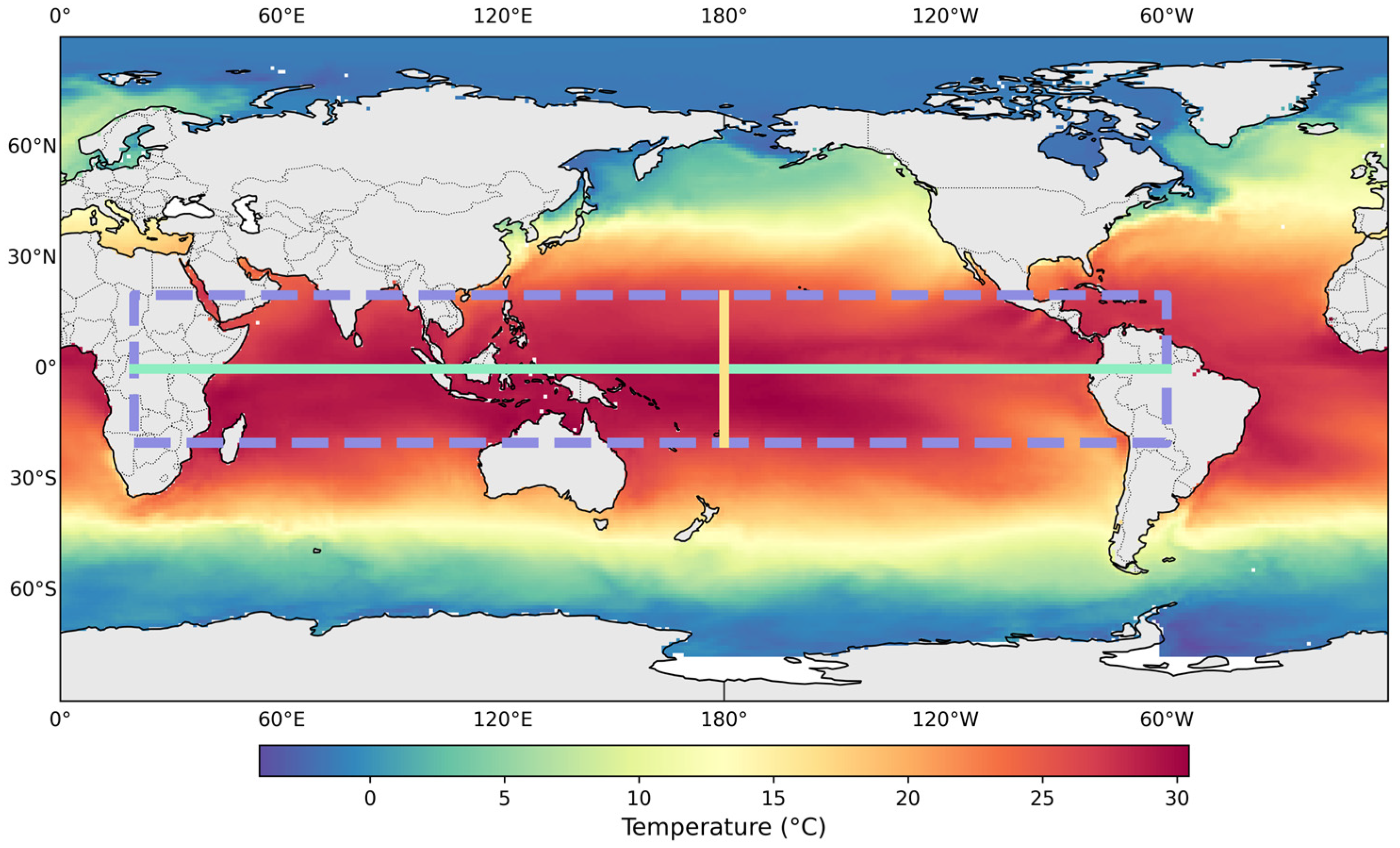
Figure 1. SST (sea surface temperature) averaged from 2010 to 2019. The study area is outlined by the box. The yellow and green lines represent the latitude and longitude profiles used in Section 5.1, respectively.
Remotesensing 17 02005 g001
Figure 2. UNet model schematic diagram.
Remotesensing 17 02005 g002
Figure 3. VI-UNet model schematic diagram.
Remotesensing 17 02005 g003
Figure 4. Layer-averaged temperature (°C) from 1–6000 m: IAP data (left) and reconstruction from the VI-UNet model with SWH inputs (right). Results are also averaged over the year 2018.
Remotesensing 17 02005 g004
Figure 5. Depth profiles of temporally and regionally averaged temperature reconstruction performance metrics for 2018 across different models (UNet and VI-UNet), with and without SWH. (a) RMSE (°C) and (b) RMSE difference (°C) relative to UNet (no swh), with negative values indicating improved reconstruction accuracy. (c,d) Difference in NRMSE (%), with negative values indicating improvement in performance. (e) Depth distribution of R2, with 1–600 m shown on the left y-axis, and 1000–5000 m shown on the right y-axis.
Remotesensing 17 02005 g005
Figure 6. Comparison of temperature reconstruction performance across different models (UNet and VI-UNet) with/without SWH: (a) spatial distribution of full-depth-averaged NRMSE; (b) spatial distribution of each layer-averaged RMSE (°C) at different depths.
Remotesensing 17 02005 g006
Figure 7. Layer-averaged salinity (psu) from 1–6000 m: IAP data (left) and VI-UNet model results with SWH inputs (right). Salinity is also averaged over the year 2018.
Remotesensing 17 02005 g007
Figure 8. Depth profiles of temporally and regionally averaged salinity reconstruction performance metrics for 2018 across different models (UNet and VI-UNet), with and without SWH. (a) RMSE (psu) and (b) RMSE difference (psu) relative to UNet (no swh), with negative values indicating improved reconstruction accuracy. (c,d) Difference in NRMSE, with negative values indicating improvement in performance. (e) Depth distribution of R2, with 1–600 m shown on the left y-axis, and 1000–5000 m shown on the right y-axis.
Remotesensing 17 02005 g008
Figure 9. Comparison of salinity reconstruction performance across different models (UNet and VI-UNet) with/without SWH: (a) spatial distribution of full-depth-averaged NRMSE; (b) spatial distribution of each layer-averaged RMSE (psu) at different depths.
Remotesensing 17 02005 g009
Figure 10. Temperature (a) and salinity (b) profiles at longitude 180° (left column) and latitude 0° (right column), averaged over the year 2018, are based on IAP data and VI-UNet (SWH) reconstructions.
Remotesensing 17 02005 g010
Figure 11. Difference profiles of temperature (upper) and salinity (lower) at 180°E (left column) and 0°N (right column), averaged over 2018, between IAP data and VI-UNet (SWH) reconstructions.
Remotesensing 17 02005 g011
Figure 12. Temperature (°C) distribution maps from 20–200 m for February, May, August, and November 2018: IAP data (left) and results from the VI-UNet model with SWH (right).
Remotesensing 17 02005 g012
Figure 13. Temperature (°C) distribution maps from 1000–4000 m for February, May, August, and November 2018: IAP data (left) and results from the VI-UNet model with SWH (right).
Remotesensing 17 02005 g013
Figure 14. Difference of temperature (°C) between the VI-UNet model with SWH and IAP data for February, May, August, and November 2018 at (left column) 20–200 m and (right column) 1000–4000 m.
Remotesensing 17 02005 g014
Figure 15. 2018 ONI (Oceanic Niño Index) and DMI (Dipole Mode Index) indices alongside the regional and depth mean RMSE of VI-UNet (SWH) temperature reconstructions (1–6000 m) over 20°S–20°N, 20°E–300°E/60°W.
Remotesensing 17 02005 g015
Table 1. Experimental design includes input and output.
ExperimentsInputsOutputs
UNet/VI-UNet (no swh)SST, SSS, SSW, SSH3D Temperature/Salinity
UNet/VI-UNet (swh)SST, SSS, SSW, SSH, SWH
Disclaimer/Publisher’s Note: The statements, opinions and data contained in all publications are solely those of the individual author(s) and contributor(s) and not of MDPI and/or the editor(s). MDPI and/or the editor(s) disclaim responsibility for any injury to people or property resulting from any ideas, methods, instructions or products referred to in the content.