A Comparative Study of Deep Semantic Segmentation and UAV-Based Multispectral Imaging for Enhanced Roadside Vegetation Composition Assessment

Abstract

Roadside vegetation composition assessment is essential to maintain ecological stability, control invasive species, and ensure the adoption of environmental regulations in areas surrounding active roadside construction zones. Traditional monitoring methods involving visual inspections are time-consuming, labor-intensive, and not scalable. Remote sensing offers a valuable alternative to automating large-scale vegetation assessment tasks efficiently. The study compares the performance of proximal RGB imagery processed using deep learning (DL) techniques against the vegetation indices (VIs) extracted at higher altitudes, establishing a foundation to use the prior in performing vegetation analysis using unmanned aerial vehicles (UAVs) for broader scalability. A pixel-wise annotated dataset for eight roadside vegetation species was curated to evaluate the performance of multiple semantic segmentation models in this context. The best-performing MAnet DL achieved a mean intersection over union of 0.90, highlighting the model’s capability in composition assessment tasks. Additionally, in predicting the vegetation cover—the DL model achieved an R² of 0.996, an MAE of 1.225, an RMSE of 1.761, and an MAPE of 3.003% and outperformed the top VI method of SAVI, which achieved an R² of 0.491, an MAE of 20.830, an RMSE of 23.473, and an MAPE of 59.057%. The strong performance of DL models on proximal RGB imagery underscores the potential of UAV-mounted high-resolution RGB sensors for automated roadside vegetation monitoring and management tasks at construction sites.

1. Introduction

Vegetation monitoring serves as a vital tool across multiple disciplines, from forest decline and carbon sequestration to climate impact assessment on plant communities [1]. Systematic observation helps detect early signs of ecological shifts, assess biodiversity fluctuations, and guide conservation efforts, particularly as human activities and climate change continue to threaten natural habitats [2]. In transportation infrastructure, monitoring roadside vegetation is essential for ensuring road safety, maintaining environmental stability, and preserving infrastructure integrity [3]. Moreover, vegetation monitoring is critical for construction site stabilization. Regulatory frameworks, such as the Construction General Permit, require that disturbed sites establish a permanent stand of vegetation at a prescribed density to prevent soil erosion and sediment runoff before project closure. Failure to meet these vegetation standards can delay permit termination, increase project costs, and jeopardize compliance with environmental regulations. Effective roadside vegetation management relies on accurate species identification, which supports strategic maintenance and targeted control efforts [4]. Managing vegetation along active roadside transportation corridors is challenging, as species introduced through construction materials, erosion control methods, or nearby land use often lack natural controls, resulting in rapid growth [5]. The unrestrained growth can obstruct visibility, elevate fire risks, and jeopardize roadway safety, leading to increased maintenance expenses and reducing the ecological benefits of managed vegetation [6]. Furthermore, transportation corridors frequently harbor invasive plant species that tend to overwhelm and replace native vegetation. When left unmanaged, these invasive vegetation species can diminish ecosystem diversity, modify wildfire patterns through accumulated dry plant material, and decay soil quality by interfering with nutrient cycling and compromising erosion protection [7]. Conventional vegetation assessment methods rely on resource-intensive field surveys involving subjective visual evaluation, requiring substantial personnel and introducing observer variability [8]. To overcome these limitations, modern approaches are needed to replace traditional methods with advanced techniques that offer greater speed, accuracy, and reliability.

Remote sensing has emerged as a key tool for vegetation monitoring, offering essential data on plant health, land cover changes, and ecosystem patterns [9]. The use of advanced sensors on satellites and unmanned aerial vehicles (UAVs) allows for early problem detection, quantitative assessment, and species identification, enabling proactive vegetation management. These approaches assist organizations in maximizing their resource allocation, adhering to statutory requirements, and advancing ecological objectives [10]. Advancements and improvements in spatial, spectral, and temporal resolution have boosted the ability to monitor plant growth patterns for multiple practical purposes [11]. Low-altitude drone imagery provides high-resolution data for detailed local monitoring, avoiding problems like cloud cover that affect satellites, while satellite imagery remains valuable for regional and global vegetation tracking [12,13]. With the availability of advanced digital sensors capable of capturing high-resolution spectral and spatial information, new opportunities have emerged for tackling complex tasks such as detailed vegetation detection and classification. However, a research gap remains in systematically evaluating whether high-resolution imagery can effectively perform vegetation composition analysis.

Multispectral imaging plays a pivotal role in vegetation monitoring by capturing reflectance across various spectral bands, including near-infrared (NIR), red, green, blue, and red edge. This enables the generation of vegetation indices (VIs) to assess plant health, chlorophyll content, and vegetation density, supporting applications such as species detection, land cover classification, and precision agriculture [14]. Multispectral data have been effectively used to distinguish between shrubs and grasses in desert environments, with machine learning models such as SVM and maximum likelihood classifiers proving particularly useful [15]. To enhance vegetation detection in urban landscapes, researchers introduced the squared red-blue NDVI, which helps reduce misclassification caused by non-vegetative surfaces [16]. For turfgrass monitoring, UAV-based image processing and ML techniques were utilized, including a green pixel detection method relying on the HSV color space [17]. In Mongolian grasslands, a comparative analysis of classification algorithms was conducted to estimate green vegetation cover, revealing significant variability over time [18]. Although multispectral imagery is widely applied in domains like crop health monitoring, weed detection, irrigation management, nutrient deficiency assessment, and yield estimation, it often struggles to differentiate between vegetation species with similar spectral reflectance properties.

Deep learning (DL) has emerged as a powerful tool in vegetation detection, enabling accurate classification, segmentation, and analysis of plant species, crop health, and vegetation cover [19]. A high-resolution grassland canopy cover map across China was generated by combining drone and satellite imagery, effectively addressing challenges related to limited field data and scale mismatches [20]. DL models such as CNNs, RNNs, and transformers have been widely applied to vegetation mapping by learning complex spatial and spectral patterns from high-resolution imagery [21]. To support nitrogen and feed management, researchers applied watershed segmentation techniques to estimate clover–grass cover [22]. In agriculture, DL supports tasks like crop yield prediction, disease detection, weed identification, and irrigation management [23]. A study conducted by [24] developed a grid cell-based approach for weed detection and localization to support precision herbicide applications. Semantic segmentation (SS) models, which classify each pixel in an image, are especially effective for species-level vegetation detection due to their fine-grained output. These models often use encoder–decoder architectures to reconstruct high-resolution predictions from compressed representations [25]. A comprehensive evaluation of thirty DL model combinations was conducted to estimate clover–grass ratios for optimizing dairy feed [8]. Another study trained the DeepLabV3+ model using NIR and RGB data to enhance vegetation detection performance [1]. AerialSegNet, an improved SegNet-based architecture, was shown to outperform several existing SS models [26]. Research has also demonstrated that multispectral UAV imagery yields superior classification of vegetation, bare soil, and dead matter in landslide-affected regions compared to RGB data alone [27]. However, UAV-based assessments have been found to underestimate vegetation cover in post-burn Mediterranean shrublands, particularly in areas characterized by high species richness [28].

Recent advances in DL have led to the integration of attention-based mechanisms in numerous semantic segmentation models for land cover classification [29,30,31,32,33,34]. GPINet incorporates geometric priors within a dual-branch CNN–Transformer architecture for complex scene segmentation [29], while BEDSN enhances intra-class consistency through a tightly coupled encoder and edge-aware feature extraction [30]. HSI-TransUnet applies transformer-based learning for crop mapping using high-resolution hyperspectral imagery [31]. RSMamba addresses dense prediction on very-high-resolution remote sensing images by eliminating the need for patch-based methods, preserving spatial context [32]. SAPNet introduces a synergistic attention mechanism that jointly captures spatial and channel affinities, improving segmentation accuracy across objects of varying size and distribution [33]. UNetFormer combines a lightweight ResNet18 encoder with a transformer decoder using global-local attention for fast and accurate urban scene segmentation [34]. While these models show strong performance on conventional datasets, their reliance on coarser remote sensing imagery may limit applicability to high-detail vegetation analysis from proximal UAS data.

In addition, several popular SS architectures have been applied successfully to high-resolution vegetation mapping using remote sensing data. UNet++, an enhanced version of U-Net with nested skip connections [35], has been implemented to estimate tree species distribution over extensive forested areas. PSPNet applies pyramid pooling to capture multi-scale contextual information and has been used in high-resolution vegetation mapping across various land cover types [36]. DeepLabV3+, which incorporates atrous spatial pyramid pooling in its encoder–decoder structure, has proven effective in identifying vegetation and green infrastructure in urban settings [37]. Furthermore, the DL model of MANet, which integrates multiple attention mechanisms, has delivered strong performance in fine-grained tasks such as segmenting specific tree species like elm in sparsely vegetated regions [38]. The demonstrated capabilities of these models in vegetation classification and detailed cover estimation highlight their relevance to remote sensing applications focused on vegetation composition analysis.

While current remote sensing and DL techniques have shown promise in vegetation detection and mapping tasks, several gaps remain that warrant further investigation. Most existing studies have concentrated on binary classification [39,40,41] or the detection of a limited number of vegetation classes [8,24,42], leaving the field of multi-class vegetation detection—particularly involving diverse roadside grass species—relatively underexplored. Accurately detecting and monitoring non-native, fast-spreading grasses is essential for ecosystem management and biodiversity conservation, yet it remains a complex challenge. This study aims to bridge these gaps by developing and evaluating SS models designed specifically for roadside vegetation composition assessment. The primary objectives of this research are to:

• Curate an SS dataset of proximal RGB images capturing diverse roadside vegetation species;
• Train and evaluate the performance of four DL-based SS models (UNet++, PSPNet, DeepLabV3+, and MANet) on a custom roadside vegetation dataset to assess their performance for vegetation composition assessment;
• Compare the performance of SS models and VI-based methods in estimating vegetation density, focusing on prediction accuracy and generalizability.

The outcomes of this research will enhance the understanding of vegetation dynamics, support targeted ecological interventions, and contribute to sustainable roadside management strategies.

2. Materials and Methods

2.1. Data Collection and Sources

To develop a comprehensive vegetation analysis framework, a diverse dataset through systematic data collection across multiple roadside construction sites in Alabama between July 2022 and July 2023 was established. A multi-tiered approach was employed using standardized 0.6 m × 0.6 m PVC frames as reference quadrats, which were strategically placed across the sites to ensure consistent sampling areas. These frames served as fixed boundaries for vegetation assessment and provided reference areas for both aerial and ground-based imagery. The data collection strategy incorporated multiple sensing platforms for collecting proximal RGB images included in the dataset. Skydio 2 (Skydio, San Mateo, CA, USA), equipped with a 12.3 MP camera capable of capturing 4056 × 3040-pixel images, was used for low-altitude flights at approximately 1.83 m above ground level (AGL). In addition, a DSLR camera (Canon EOS Rebel SL1 DSLR, Canon, Tokyo, Japan) with an 18.5 MP sensor producing images at 5288 × 3506 pixels was used at a similar altitude for ground-based RGB image collection. The ground sampling distance (GSD) of the Skydio drone and DSLR camera was 0.0138 cm/pixel and 0.0139 cm/pixel, respectively. This close-range proximal imagery was instrumental in training DL models for vegetation detection and composition assessment, providing detailed visuals necessary to differentiate between multiple roadside vegetation species. A total of 18 UAV flights, along with ground-based data collection, were conducted over a 13-month period during the data collection phase. The dataset comprises eight different roadside grass species, which were collected during data collection across several active roadside construction sites in Alabama. The dataset covers eight grass species, including annual ryegrass (Lolium multiflorum), bahia (Paspalam notatum), bermuda (Cynodon dactylon), crabgrass (Digitaria sanguinalis), browntop millet (Urochloa ramosa), lespedeza (Lespedeza striata), johnsongrass (Sorghum halepense), and fescue (Festuca arundinacea). The visual resemblance between various grass species, as illustrated in Figure 1, highlights the importance of employing advanced classification techniques for accurate and reliable species-level differentiation.

Table 1. Data collection summary.

Location	Date	Vegetation Species	Image Acquisition: Images Collected
Lee County: Auburn	10 March 2023	Annual ryegrass	Skydio: 10
	16 March 2023	Annual ryegrass and Lespedeza	Skydio: 39
	23 March 2023	Annual ryegrass, Bermuda, Lespedeza	Canon: 25
Lee County: Opelika	08 July 2022	Bermuda, Crabgrass, Johnsongrass, Lespedeza	Canon: 38. Skydio: 40
	15 July 2022	Bermuda, Browntop millet, Crabgrass, Johnsongrass, Lespedeza	Canon: 40. Skydio: 40
	22 July 2022	Bahia, Bermuda, Browntop millet, Crabgrass, Johnsongrass, Lespedeza	Canon: 40. Skydio: 39
	29 July 2022	Bahia, Bermuda, Browntop millet, Lespedeza	Canon: 15
	03 August 2022	Browntop millet, Crabgrass, Johnsongrass, Lespedeza	Canon: 40, Skydio: 33
	11 August 2022	Browntop millet, Crabgrass, Johnsongrass, Lespedeza	Canon: 40
	18 August 2022	Browntop millet, Crabgrass, Johnsongrass, Lespedeza	Skydio: 42
	02 September 2022	Crabgrass, Lespedeza	Skydio: 30
	26 May 2023	Bermuda	Canon: 10
	02 June 2023	Bermuda	Canon: 20
	18 July 2023	Bahia, Lespedeza	Canon: 20
Linden	28 July 2023	Bahia, Browntop millet, Crabgrass Johnsongrass, Lespedeza	Canon: 16
Montgomery	09 June 2023	Annual ryegrass, Johnsongrass, Lespedeza	Canon: 20
Prattville	27 July 2023	Bermuda, Crabgrass, Johnsongrass, Lespedeza	Canon: 20
Tuscaloosa	28 July 2023	Crabgrass, Lespedeza	Canon: 18

and Figure 2 provide a comprehensive overview of the UAV flight operations and the specific site locations where data were collected.

In addition, multispectral data were collected using a DJI Matrice 600 pro (DJI Technology Inc., Shenzhen, China) UAV equipped with a Sentera 6X sensor (Sentera, St. Paul, MN, USA), which was flown at an altitude of 30 m AGL. The multispectral sensor collected imagery across five different bands of red, green, blue, near-infrared (NIR), and red edge, respectively. This information was utilized to evaluate the effectiveness of individual spectral bands for determining vegetation cover density by deriving various VIs. The multispectral bands of the Sentera 6X sensor provided a spatial resolution of 3.2 MP, producing images sized at 2048 × 1536 pixels with a GSD of 1.3 cm/pixel. Figure 3 presents images of the different cameras and drones used for data collection. To analyze vegetation cover using multispectral data, several UAV flights were conducted at multiple roadside construction sites in Alabama, including Prattville, Tuscaloosa, Linden, and Opelika.

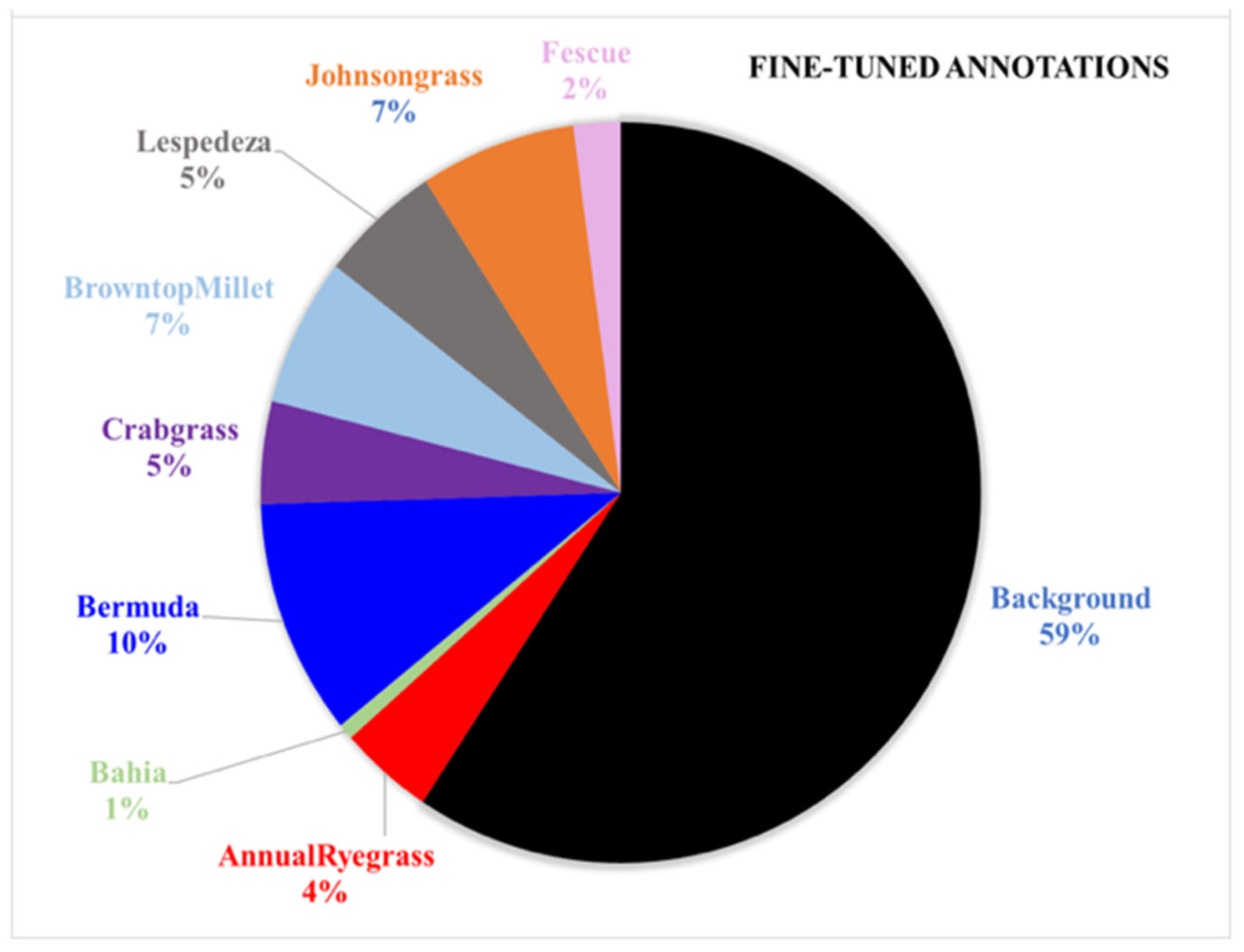
2.1.1. Image Annotations

The SS-based DL models were trained using the RGB images alone. Training these models requires a pixel-wise annotated dataset where each and every pixel is labeled to represent a specific class category. All the RGB images in the dataset were annotated using the ‘COCO Annotator’ tool [43], which provides a straightforward interface for creating detailed, pixel-level annotations. A ‘.json’ file was generated after completing the annotations, containing the metadata needed to link each pixel to a specific vegetation class. Image annotation was restricted to vegetation species located within the established PVC frame boundaries for focused data annotation and analysis. These predefined sampling areas created a structured framework for assessing DL model accuracy in vegetation species identification and classification. The frame-based annotation strategy ensured precise evaluation of model performance within clearly defined spatial boundaries.

During the annotation process, it was observed that a significant portion of the images contained areas outside the region of interest or PVC frame boundaries, as shown in Figure 4. To ensure optimal model training, a Python (version 3.9.18) script was employed to extract only the regions within the frame from both the original images and the corresponding annotated masks. This process resulted in a refined dataset of 635 images, each focused solely on the relevant frame area. Isolating the frame areas also led to a reduction in image dimensions, with ground-based images reduced to 3072 × 2560 pixels and Skydio UAV images reduced to 768 × 768 pixels, respectively. All 635 original images were divided into smaller 256 × 256-pixel tiles, which were subsequently utilized for SS-based DL model training. Following this tiling process, the final training dataset comprised 44,793 images.

2.1.2. Image Pre-Processing

Following the reduction of image dimensions and the extraction of frame regions, it was observed that the annotations lacked precision, with numerous background pixels mistakenly labeled as vegetation species. Accurate and high-quality annotations are essential for training effective SS models, as they enable the model to learn meaningful features and enhance classification accuracy during evaluation. Conversely, poor annotation quality can severely hinder model performance and compromise its ability to generalize well to unseen datasets. To address this issue, a strategy was implemented to refine the annotations. The refinement strategy involved a two-step approach. The OpenCV library [44] was used to isolate the green pixels from the original image, and the green-pixel image was then compared with the original annotated mask; any pixels that were not identified as green but were labeled as a vegetation class were reclassified as background class. This adjustment resulted in cleaner and more accurate annotations, focusing solely on true vegetation pixels. As shown in Figure 5, this refinement process helped to improve annotation quality, resulting in fine-tuned annotations that were better suited for training the DL models.

The pie chart in Figure 6 illustrates the pixel percentage distribution of various grass species used for training the SS-based DL model. The majority of the dataset consists of background pixels, accounting for 59% of the total, followed by bermuda grass at 10%. Other grass species, including johnsongrass (7%), browntop millet (7%), lespedeza (5%), crabgrass (5%), and fescue (2%), are represented in smaller proportions. Annual ryegrass and bahia have the smallest shares, contributing 4% and 1%, respectively. This distribution reflects the diverse composition of the dataset and highlights the class imbalance that the model needs to address during training. The pie charts depicting pixel percentage share before and after fine-tuning the annotations are presented and discussed with details in Section Text S1 of the Supplementary Materials.

The DL model was trained on an annotated dataset of 44,793 images, each sized 256 × 256 pixels. The dataset was split into three parts: training, validation, and testing sets, with a ratio of 70%, 15%, and 15%, respectively. To prevent data leakage, all image tiles from the same source frame were assigned exclusively to a single dataset partition, ensuring no shared spatial context between sets and maintaining dataset independence for reliable model evaluation. This division resulted in 31,357 images for training, 6718 images for validation, and testing datasets. The training set was used to optimize the model’s parameters, while the validation set provided feedback on model performance during training, helping to prevent overfitting. The testing set, containing unseen data, was reserved for final evaluation to assess the model’s ability to generalize to new images. This structured data division enabled a robust evaluation framework, ensuring that the model’s performance could be accurately measured.

2.2. Deep Learning Model Training

In this study, the encoder–decoder based SS models of U-Net++, PSPNet, MAnet, and DeepLavV3+ were explored to perform roadside vegetation composition assessment tasks.

The U-Net++ model enhances the original U-Net architecture by introducing nested and dense skip connections, which improve segmentation accuracy by refining feature maps at multiple scales [45]. This architecture is particularly effective for tasks requiring precise boundary delineation, such as medical and vegetation segmentation. PSPNet uses pyramid pooling to capture global and local contextual information, which helps improve segmentation accuracy in complex scenes. It is widely used in applications that benefit from understanding spatial hierarchies, such as urban and natural landscape segmentation [46]. MAnet integrates multi-scale attention mechanisms with U-Net, enabling the model to focus on different parts of the image at varying scales. This improves its ability to detect fine details and capture spatial context, making it suitable for tasks with intricate object boundaries [47]. DeepLabV3+ combines atrous spatial pyramid pooling with a decoder module, allowing it to capture contextual information while preserving high spatial resolution. It has been successfully applied in tasks requiring both fine detail and global context, such as satellite and vegetation segmentation [48].

As illustrated in Figure 6, the fine-tuned dataset exhibited substantial class imbalance in pixel distribution across different vegetation species. The distribution showed background (59%), bermuda (10%), johnsongrass (7%), and browntop millet (7%) as dominant classes, while several important grass species such as fescue (2%) and bahia (1%) were significantly underrepresented. This imbalance posed a critical challenge for model training, potentially biasing the model toward majority classes and compromising its ability to accurately detect and classify minority species. To overcome this class imbalance challenge, the focal loss function was implemented during model training. Focal loss, introduced by [49], effectively handles class imbalance by dynamically adjusting the weight of each class based on classification difficulty. This loss function reduces the relative loss contribution from well-classified examples and focuses training on hard-to-classify cases, particularly benefiting the underrepresented grass species. The adaptive nature of focal loss helps prevent the model from being dominated by prevalent classes while maintaining learning efficiency for minority classes.

Model training was conducted on a Dell Precision 5680 laptop (Dell, Round Rock, TX, USA) running Windows 11 Enterprise (Windows, Redmond, CA, USA). The system specifications included an Intel Core i9-12900H processor, 32 GB LPDDR5 RAM, 1 TB NVMe SSD storage, and an Nvidia GeForce RTX 4090 GPU with 16 GB GDDR6 memory. The SS models utilized various architecture backbones implemented through ‘PyTorch’, optimized with Nvidia CUDA 11.8 and OpenCV 4.8.0 for GPU-accelerated training. The dataset consisted of 44,793 images, each sized at 256 × 256 pixels. The specific hyperparameters employed for each model variant are detailed in

Table 2. Hyperparameters used to train DL models.

Hyperparameters	Values
Optimizer	Adam
Loss function	Focal loss (ɤ = 3.0)
Learning rate scheduler	CosineAnnealingLR
Epochs	50
Augmentations	Random Crop, Horizontal/Vertical flip, Shift scale rotate
Batch size	32
Image size	256 × 256
Evaluation metrics	Loss, Precision, Recall, IoU
Weight initialization	Fine-tuning pretrained weights on ImageNet
Architecture backbones	mit_b5, mit_b4, ResNet101, ResNet50, Xception
Dropout rate	0.2
Learning rate	2 × 10−4

.

The SS models were evaluated using four fundamental metrics: precision, recall, intersection over union (IoU), and mIoU on the validation datasets during training. Mean precision quantifies prediction accuracy by measuring the ratio of correct positive predictions to total positive predictions, while mean recall assesses detection completeness by calculating the proportion of actual positive cases correctly identified. The IoU score, calculated as the intersection area divided by the union area between predicted and ground truth segmentation masks, serves as the primary evaluation metric for SS tasks. IoU significance stems from its ability to simultaneously assess both localization accuracy and segmentation quality, making it particularly valuable for pixel-wise classification tasks. Lastly, mIoU extends the IoU metric by averaging the IoU scores across all classes, providing a measure of overall segmentation performance. Mathematically, these metrics can be represented as follows:

$$\mathit{Precision}={\displaystyle \frac{1}{N}}{\sum }_{i=1}^N{\displaystyle \frac{{TP}_i}{({TP}_i+{FP}_i)}}$$

(1)

$$\mathit{Recall}={\displaystyle \frac{1}{N}}{\sum }_{i=1}^N{\displaystyle \frac{{TP}_i}{({TP}_i+{FN}_i)}}$$

(2)

$${IoU}_i ={\displaystyle \frac{{TP}_i}{({TP}_i+{FP}_i+{FN}_i)}}$$

(3)

$$\mathit{Mean}\mathit{IoU}={\displaystyle \frac{1}{N}}{\sum }_{i=1}^N{IoU}_i$$

(4)

where TP (True Positive) refers to correctly predicted pixels of class i, FP (False Positive) refers to pixels incorrectly predicted as class i, FN (False Negative) refers to pixels of class i incorrectly predicted as another class, and N refers to the total number of classes. Precision, recall, IoU, and mean IoU (mIoU) were selected as the primary evaluation metrics due to their effectiveness in assessing performance in multi-class SS tasks on the validation datasets. These evaluation metrics offer additional insights into the model’s ability to correctly identify minority and majority classes. Metrics like F1-score and overall accuracy were not emphasized, as they may not fully capture model behavior in the presence of class imbalance.

Following the evaluation of the DL models on the validation datasets, performance assessment was conducted on an independent testing dataset by generating confusion matrices to evaluate classification accuracy across multiple roadside vegetation species. To facilitate a clearer interpretation of results, normalization along the columns of the confusion matrices was applied to represent the model’s precision for each predicted class. This approach enables a direct evaluation of prediction accuracy for each class, which is important in understanding the performance of DL models on multi-class SS tasks that involve visually similar or underrepresented vegetation species.

2.3. Vegetation Detection Using Vegetation Index-Based Methods

The NIR band was particularly valuable, as it provides insights into chlorophyll content, a key indicator of plant health and vitality. The multispectral data enabled the generation of several VI, which are crucial for accurately estimating vegetation cover in the study areas.

Three different VIs were derived and explored in this research work. The normalized difference vegetation index (NDVI) is a widely used indicator that leverages the NIR and red bands to estimate vegetation health and chlorophyll content, making it suitable for general vegetation density assessment. The normalized difference red edge (NDRE) index utilizes the red-edge band instead of the red band, offering increased sensitivity to chlorophyll concentration and better performance in areas with dense or mature vegetation, and the soil adjusted vegetation index (SAVI) incorporates a soil brightness correction factor, which makes it more effective in areas with sparse vegetation or exposed soil, by reducing the influence of background soil reflectance. Each of these indices offers unique advantages for vegetation analysis:

$$\mathit{NDVI}={\displaystyle \frac{(NIR-Red)}{(NIR+Red)}}$$

(5)

$$\mathit{NDRE}={\displaystyle \frac{(NIR-RedEdge)}{(NIR+RedEdge)}}$$

(6)

$$\mathit{SAVI}={\displaystyle \frac{(NIR-Red)\times (1+L)}{(NIR+Red+L)}}, L=0.25$$

(7)

The steps followed for processing multispectral images for the task of vegetation detection are depicted in Figure 7. The raw multispectral images were first calibrated to ensure accurate reflectance values, and then orthomosaics were generated for the key spectral bands using photogrammetry software (Agisoft Metashape Professional^TM version 2.0.4, St. Petersburg, Russia). Next, NDVI, NDRE, and SAVI were calculated for each orthomosaic using the ‘Raster Calculator’ feature in QGIS (QGIS Desktop 3.40.3, QGIS Documentation tool, 2024). The orthomosaics were then imported into QGIS, where the frames placed during data collection were segmented, allowing for focused analysis within the designated boundaries. To determine vegetation cover within the frames, various thresholds were applied to the generated VI, with NDVI thresholds ranging from 25% to 60%, NDRE from 20% to 45%, and SAVI from 20% to 55%. Finally, the zonal statistics tool in QGIS was used to calculate the mean statistic for each frame, enabling an accurate assessment of vegetation cover at the frame level. This methodical approach to vegetation analysis, utilizing multispectral data and VIs, enabled precise detection and assessment of vegetation cover, facilitating better understanding and management of vegetation at the study sites.

The evaluation framework for comparing VI-based approaches and the optimal DL model incorporated multiple quantitative metrics on the test dataset: mean absolute error (MAE), root mean squared error (RMSE), mean absolute percentage error (MAPE), and coefficient of determination (R²). Statistical validation of the prediction accuracy was conducted using Bland–Altman (B–A) analysis [50] to assess the level of agreement between the prediction method and manual annotation method for vegetation cover assessment. The B–A methodology quantifies prediction reliability through two key parameters: bias (mean difference between actual and predicted values) and limits of agreement (LoA, defined as bias ± 1.96 standard deviations with a 95% confidence interval). This analysis provides critical insights into model performance, where minimal bias and narrow LoA ranges indicate strong predictive accuracy. B–A plots offer a visual representation of measurement differences against means, facilitating the identification of systematic biases and agreement boundaries essential for model validation. MAE, RMSE, MAPE, and R² were evaluated using the following equations:

$$\mathit{MAE}={\displaystyle \frac{1}{N}}{\sum }_{i=0}^{N-1}\left(y_i-y_i^{pred}\right)$$

(8)

$$\mathit{RMSE}=\sqrt{{\displaystyle \frac{1}{N}}{\sum }_{i=0}^{N-1}{\left(y_i-y_i^{pred}\right)}^2}$$

(9)

$$\mathit{MAPE}={\displaystyle \frac{1}{N}}\left({\sum }_{i=0}^{N-1}{\displaystyle \frac{\left|y_i-y_i^{pred}\right|}{y_i}}\times 100\right)$$

(10)

$$R^2=1-{\displaystyle \frac{{\sum }_{i=0}^{N-1}{\left(y_i-y_i^{pred}\right)}^2}{{\sum }_{i=0}^{N-1}{\left(y_i-y_{mean}\right)}^2}}$$

(11)

3. Results

3.1. Deep Learning Model Performance

The performance evaluation of different SS models revealed varying capabilities in vegetation detection tasks. Four distinct architectures were assessed: UNet++, PSPNet, DeepLabV3+, and MAnet, each utilizing different backbone networks in their encoder sections. The evaluation metric scores for various DL models evaluated on the validation dataset are summarized in

Table 3. Mean evaluation metric scores of DL models on the validation dataset.

DL Model	Encoder	Loss	Precision	Recall	mIoU	Trainable Parameters
UNet++	ResNet50	0.002	0.608	0.661	0.688	48.98 M
PSPNet	mit_b5	0.001	0.664	0.712	0.751	81.63 M
DeepLabV3+	ResNet101	0.001	0.623	0.700	0.779	45.67 M
MAnet	mit_b4	0.001	0.681	0.737	0.791	54.84 M

. Each model was assessed based on key metrics: loss, precision, recall, and mIoU score. These metrics collectively provide insights into the model’s accuracy, reliability, and ability to generalize to new data.

The encoder section of each model plays a crucial role in feature extraction. It utilizes different backbone architectures to capture intricate details from input images, significantly influencing the model’s overall performance. The UNet++ model, equipped with a ResNet50 backbone, delivered acceptable results but recorded the lowest mIoU score (0.688) among the evaluated models. Although ResNet50 is known for its efficiency in segmentation tasks, the absence of transformer-based modules may have constrained its effectiveness for this particular application. The PSPNet model with a mix vision transformer (mit_b5) backbone performed well, yielding an mIoU score of 0.751 and maintaining good precision and recall values. MiT architectures are well-suited for handling complex image segmentation tasks, as they leverage transformer blocks to capture long-range dependencies and richer contextual information across the image. In this case, the MiT architecture in PSPNet enhanced its ability to capture spatial hierarchies and context within the images, although it was outperformed by MAnet in this study. The DeepLabV3+ model, equipped with a ResNet101 backbone, achieved an mIoU score of 0.779. Despite having a lower number of trainable parameters than PSPNet, DeepLabV3+ incorporates atrous spatial pyramid pooling, which allows it to better capture information at multiple spatial scales. The use of the ResNet101 backbone, which used deep residual layers along with the design advantage of the DeepLabV3+ model, may explain its superior mIoU performance, suggesting that effective context modeling and architectural efficiency can be more influential than model size alone in SS tasks. Lastly, the MAnet model, which utilized the mit_b4 architecture as its encoder backbone, achieved the best results on the validation dataset. This superior performance can be attributed to the model’s ability to combine attention mechanisms with hierarchical feature extraction, enabling precise differentiation of visually similar vegetation classes. The MAnet model with the MiT architecture backbone achieved high precision (0.681), recall (0.737), and mIoU score (0.791) on the validation dataset.

The transformer-based backbones (MiT_b4 and MiT_b5) demonstrated superior performance in segmentation tasks, particularly the MAnet model, which achieved the highest accuracy and segmentation quality on the validation dataset. These results highlight the potential of transformer-based architectures in enhancing the performance of SS models in applications involving vegetation detection and classification. The enhanced performance can be attributed to the MiT backbone, which integrates convolutional layers with transformer-based attention mechanisms. This hybrid architecture enables the model to capture both fine-grained local features and broader contextual information. These capabilities are particularly valuable in complex roadside environments where vegetation species may be visually similar, spatially overlapping, or unevenly distributed. By modeling long-range dependencies and preserving spatial resolution, the MiT backbone significantly boosts the model’s ability to distinguish between closely related classes and contributes to its robustness.

The DL model performance was further evaluated on the testing dataset to assess generalization capability across unseen data. The UNet++ model (Figure S2 in Supplementary Materials) with a ResNet50 backbone achieves an mIoU score of 0.771 for pixel-wise vegetation classification. High true-positive rates are observed for crabgrass (0.83) and lespedeza (0.80), reflecting strong performance in these classes. The background class also shows good accuracy (0.89), demonstrating its ability to separate vegetation from non-vegetation. However, lower accuracy for browntop millet (0.70) suggests challenges in distinguishing similar classes. The PSPNet model (Figure S3 in Supplementary Materials) with the mit_b5 backbone achieves an mIoU of 0.878, with high true-positive rates for bermuda (0.96) and annual ryegrass (0.93). The background class also performs well (0.95), ensuring accurate separation of vegetation from non-vegetation areas. However, lower accuracy in classes like lespedeza (0.85) and crabgrass (0.75) indicates some misclassification. The DeepLabV3+ model (Figure S4 in Supplementary Materials) with a ResNet101 backbone achieves an mIoU of 0.894, with strong performance for bermuda (0.96) and bahia (0.94). The background class also scores highly (0.95), reinforcing its ability to distinguish vegetation. However, slightly lower accuracy in crabgrass (0.75) and johnsongrass (0.87) indicates areas for improvement. Overall, the model shows reliable generalization across most vegetation classes. To provide a more detailed comparison, the class-wise prediction IoU scores of each deep learning model across the eight vegetation species are summarized in

Table 4. Class-wise prediction IoU scores of DL models using different backbones.

DL Model	Backbone	Annual Ryegrass	Bahia	Bermuda	Crabgrass	Brown Top Millet	Lespedeza	Johnsongrass	Fescue
UNet++	Resnet50	0.71	0.78	0.74	0.83	0.70	0.80	0.71	0.78
PSPnet	Mit_b5	0.93	0.87	0.96	0.75	0.90	0.85	0.83	0.87
DeepLabV3+	Resnet 101	0.94	0.94	0.96	0.75	0.84	0.87	0.87	0.93
MAnet	Mit_b4	0.97	0.96	0.95	0.75	0.90	0.84	0.86	0.91

.

The confusion matrix for the MAnet model as shown in Figure 8 with the mit_b4 backbone demonstrates high accuracy in pixel-wise classification across various vegetation classes, achieving an mIoU score of 0.9. This model shows strong performance, with notable true-positive rates for annual ryegrass (0.97) and bahia (0.96), indicating effective detection and classification of these categories. The background class also achieved a high accuracy of 0.96, essential for distinguishing vegetation from non-vegetation areas. Classes like bermuda (0.95) and browntop millet (0.9) also show high accuracy, reflecting the model’s robustness in handling diverse vegetation types. However, there are some minor misclassifications for classes like lespedeza (0.84) and crabgrass (0.75), where slight overlaps in classification are observed.

The MAnet model achieved the highest overall IoU score among all models tested, with a mean IoU of 0.90 along the diagonal values of the confusion matrix, confirming the best performance in accurately identifying each vegetation class on the testing dataset amongst other SS models explored in this study. This high IoU score indicates that the MAnet model with the mit_b4 backbone generalizes well and is particularly effective for this multi-class SS task.

Figure 9 presents a visual comparison of the predictions made by different DL models on a set of test images, highlighting their performance in vegetation classification. Among the models, the MAnet model with mit_b4 backbone demonstrates better predictions, particularly in capturing fine details and distinguishing between different vegetation classes. This is evident in its ability to accurately segment smaller patches and complex boundaries in mixed vegetation areas compared to the other models.

The DL model exhibited certain limitations in accurately distinguishing between specific vegetation species, particularly among morphologically similar grass species. As illustrated in Figure 10, notable confusion occurred between johnsongrass, crabgrass, and browntop millet, where the model occasionally misclassified these species as one another. This performance limitation can be primarily attributed to the high degree of visual similarity among these grass species, which share comparable physical characteristics in terms of blade structure, color, and growth patterns. In contrast, the model demonstrated superior performance in detecting and classifying grass species with more distinctive morphological features, such as lespedeza, bahia, bermuda, and fescue, as shown in Figure 8. These species possess unique visual characteristics that enable more reliable differentiation, resulting in more accurate classification outcomes. This observation highlights the model’s strength in distinguishing vegetation species with distinct features while acknowledging its current limitations in differentiating between visually similar grass types, suggesting potential areas for future model refinement and enhancement.

3.2. Vegetation Detection Using Vegetation Index-Based Methods

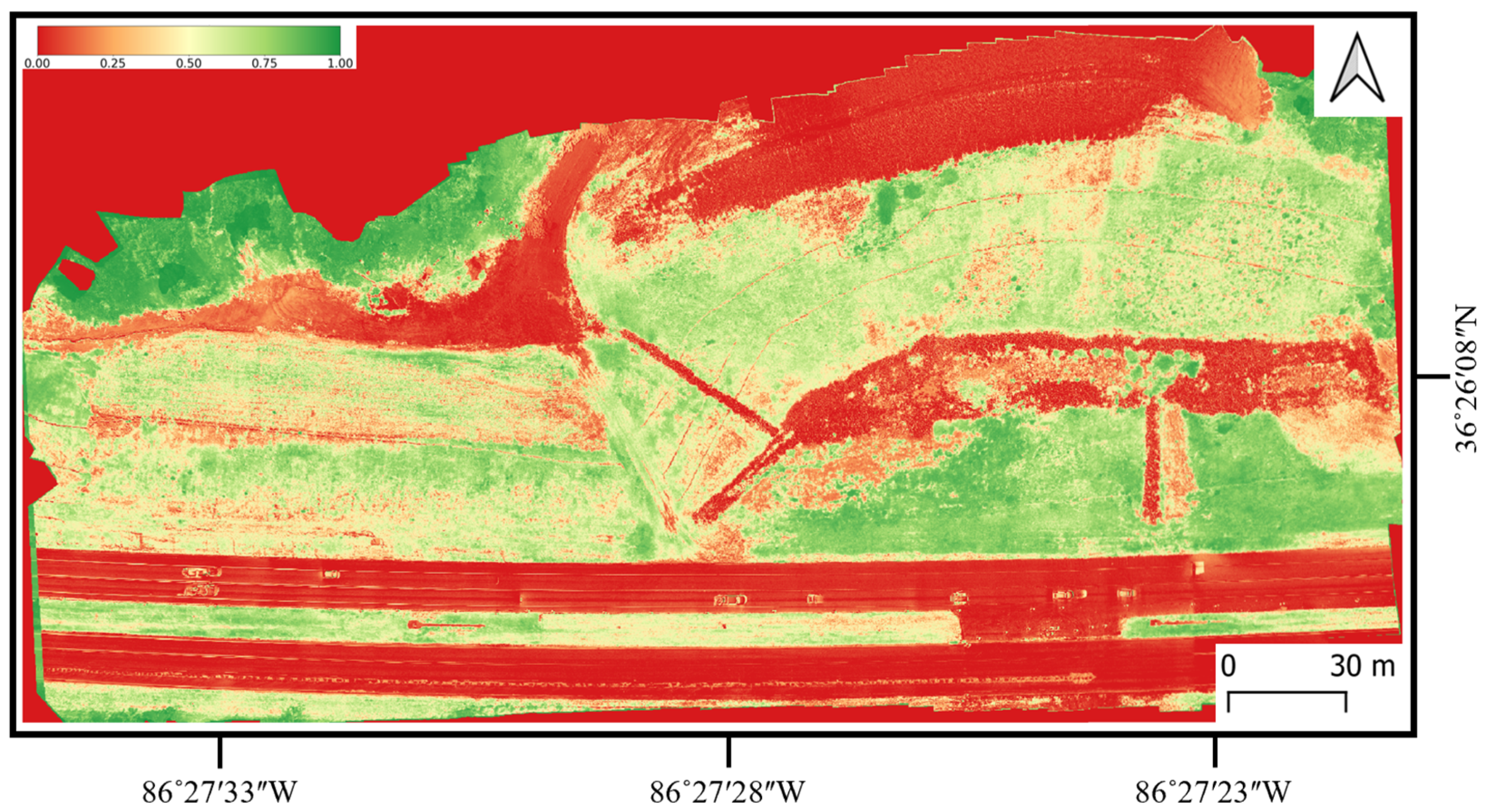
3.2.1. Vegetation Detection at Prattville Construction Site

The VI maps help measure the chlorophyll content and were then used to assess vegetation coverage at roadside construction sites. Figure 11, Figure 12 and Figure 13 represent the NDVI, NDRE, and SAVI maps, respectively, derived from combinations of NIR, red, and red-edge orthomosaics collected at the Prattville roadside construction site.

Figure 14 illustrates magnified sections of an RGB image (above) and its corresponding NDVI map (below), with each frame assigned a unique serial number. The figure highlights significant spatial variation in vegetation health, as indicated by differences in NDVI values across the frame. Green areas in the NDVI map represent higher vegetation vigor, while red areas correspond to sparse or stressed vegetation. The overlaid squares mark sampled quadrat locations, illustrating how ground truth data were aligned with spectral responses. The observed variability illustrates the challenge of reliably estimating vegetation density with VI-based approaches, especially in regions where mixed pixel effects arise due to substantial spatial heterogeneity.

The zonal statistics for the optimal thresholds of various VI used to estimate vegetation cover for Prattville roadside construction site are presented in

Table 5. Zonal statistics on selected patches at the Prattville roadside construction site.

Frame ID	Actual Vegetation Cover	Predicted Vegetation Cover: Deep Learning	Predicted Vegetation Cover: NDVI—0.5	Predicted Vegetation Cover: NDRE—0.25	Predicted Vegetation Cover: SAVI—0.40
1	0.357	0.345 (Testing)	0.667	0.713	0.646
2	0.242	0.239 (Training)	0.480	0.480	0.423
3	0.009	0.008 (Training)	0.008	0.104	0.008
4	0.257	0.264 (Training)	0.545	0.500	0.519
5	0.229	0.220 (Testing)	0.423	0.531	0.379
6	0.495	0.500 (Training)	0.930	0.885	0.886
7	0.332	0.331 (Training)	0.891	0.798	0.813
8	0.398	0.391 (Training)	0.952	0.871	0.949
9	0.357	0.363 (Training)	0.768	0.685	0.711
10	0.136	0.134 (Testing)	0.286	0.472	0.196
11	0.186	0.192 (Training)	0.478	0.450	0.282
12	0.291	0.290 (Training)	0.767	0.710	0.694
13	0.354	0.355 (Training)	0.766	0.743	0.715
14	0.338	0.335 (Training)	0.753	0.711	0.695
15	0.261	0.278 (Testing)	0.533	0.582	0.417
16	0.413	0.392 (Training)	0.870	0.878	0.870
17	0.251	0.235 (Training)	0.698	0.616	0.654
18	0.368	0.354 (Training)	0.928	0.880	0.925
19	0.304	0.307 (Training)	0.595	0.639	0.505
20	0.218	0.217 (Testing)	0.286	0.296	0.269

.

The VI orthomosaic maps and zonal statistics from the Prattville roadside construction site are presented here, while VI orthomosaics and zonal statistics for other roadside construction sites, including Tuscaloosa, Linden, and Opelika, are presented and discussed in Section Text S3 of the Supplementary Materials.

3.2.2. Determining Optimal Thresholds for Vegetation Detection Using Vegetation Indices Methods

The NDVI values were standardized with a range of 0 to 1 for consistent interpretation across all study sites. In order to analyze the vegetation coverage, multiple threshold-based analyses were performed on the NDVI maps, exploring values between 25% and 60%. This multi-threshold approach was essential as different NDVI values correspond to varying levels of vegetation health and density. The primary objective of exploring multiple thresholds was to identify an optimal threshold value that would yield vegetation predictions closely matching the actual vegetation cover observed in the original frame annotations at the roadside construction sites. The optimal threshold of 50% yielded a higher R² of 0.193, an MAE of 28.020, an RMSE of 32.153, and an MAPE of 73.567%, demonstrating improved prediction accuracy for NDVI. A scatterplot illustrating the performance of this threshold in predicting vegetation cover versus actual vegetation cover is shown in Figure 15.

Similarly, multiple threshold values were explored for NDRE maps, ranging from 20% to 50%. This narrower range was observed due to the generally lower pixel values in NDRE compared to other VIs, with fewer pixels exceeding values above 0.5 or 50% during analysis. An optimal threshold of 25% for NDRE achieved an improved R² of 0.224, an MAE of 26.906, an RMSE of 30.722, and an MAPE score of 87.012%. Figure 16 presents a scatterplot showing the performance of this threshold in predicting vegetation cover versus actual vegetation cover.

Similarly, analysis of the threshold values between 20% and 55% revealed that a 40% threshold for SAVI achieved an optimal performance, with an R² of 0.239, an MAE of 24.263, an RMSE of 29.003, and an MAPE of 62.787%, indicating enhanced prediction accuracy. Figure 17 presents a scatterplot showing the performance of this threshold in predicting vegetation cover versus actual vegetation cover.

Among all VI methods and their respective thresholds, the SAVI method at the 40% threshold demonstrated the best performance in predicting vegetation cover at roadside construction sites. The performance of this optimal SAVI threshold configuration was subsequently compared with the best-performing DL model, MAnet, through comprehensive statistical analysis, which is presented in the following section.

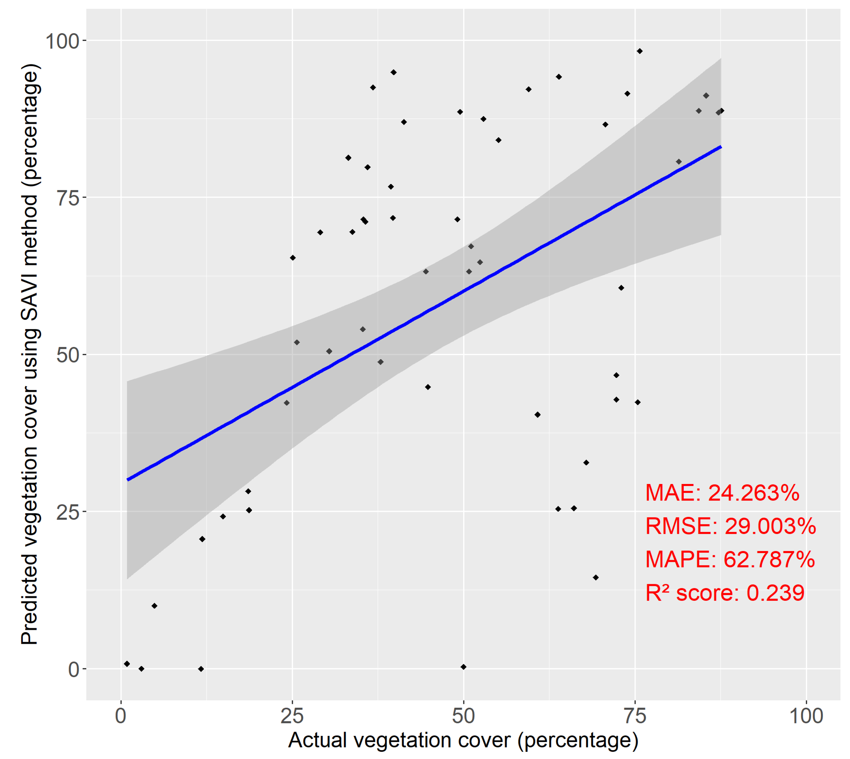
3.3. Performance Assessment: Comparison of Vegetation Detection Using Vegetation Indices and Deep Learning Approaches

A comparative analysis was conducted to assess the performance of the VI-based and DL models in estimating vegetation cover. The best-performing VI method, SAVI with a 40% threshold, was used to estimate vegetation cover on the test dataset.

The B–A plot for the VI-based approach revealed a bias or mean difference of 5.220 with a standard deviation of 23.480, and LoA extending from −40.800 to 51.240. The significant slope of 0.476 (p-value < 0.05) suggests that the bias is not constant and varies across the range of vegetation cover values, indicating a proportional bias in the predictions. This was further supported by the scatter plot, which showed an R² of 0.491, along with a high MAE of 20.830, an RMSE of 23.473, and an MAPE of 59.057%, reflecting moderate alignment with the actual vegetation cover measurements (Figure 18).

In contrast, the DL model performed significantly better than the VI-based approach (Figure 19). The B–A plot for the DL model revealed a mean difference of only 1.125, with a significantly lower standard deviation of 1.390 and LoA ranging from −1.599 to 3.849. The scatter plot for the DL model indicated a near-perfect fit, with an R² of 0.996, an MAE of 1.225, an RMSE of 1.761, and an MAPE of 3.003%. These results indicate that the DL model provided an accurate and consistent vegetation cover estimate with minimal prediction errors. The comparison strongly suggests that the DL model outperforms the VI-based approach in estimating vegetation cover, offering a more reliable tool for applications in environmental monitoring and vegetation management.

Overall, the DL model significantly outperformed the VI-based approach in estimating vegetation cover. The DL model’s ability to capture complex patterns and relationships within the data led to more accurate and consistent predictions. These findings suggest that DL models hold great potential for advancing vegetation monitoring and management practices.

4. Discussion

Gaining insights into the composition of roadside vegetation is essential for understanding species distribution and ecological roles, enabling timely management interventions to control growth and protect native biodiversity. This knowledge is vital for making informed decisions in sustainable land use and environmental planning. Remote sensing technologies, combined with DL models, offer powerful tools to efficiently monitor, analyze, and map vegetation composition over large areas effectively. SS-based DL algorithms perform detailed pixel-level classification, allowing for more accurate and nuanced analysis of vegetation species and distributions. The DL models developed in this study, especially MAnet with a transformer-based backbone, showed excellent accuracy, achieving an R² score of 0.996 for vegetation cover prediction, along with a mean IoU score of 0.90, indicating strong generalization for composition assessment tasks. This pixel-level classification capability supports its practical utility in real-world applications like vegetation monitoring on roadside construction sites and biodiversity conservation in similar environments. While the model demonstrated robust performance in distinguishing most vegetation species, it exhibited some limitations in differentiating between morphologically similar grass species. In particular, instances of misclassification were observed among visually similar species such as johnsongrass, crabgrass, and browntop millet due to their comparable physical characteristics. These findings align with similar challenges reported by [5], where comparable misclassification patterns were observed when using XGBoost models on UAV-captured RGB imagery at an altitude of 70 m for grass species detection. This consistent pattern across different methodologies suggests that the challenge of distinguishing between visually similar grass species remains a fundamental limitation in remote sensing-based vegetation classification. The findings are consistent with those of [51], who applied UAV imagery and SS models, including ResNet, to detect invasive grassland species, achieving an mIoU of 85%. While similar in accuracy, the MAnet model used in this study demonstrated improved generalization, reaching a higher IoU score of 0.90. Both approaches highlight the effectiveness of DL models for detailed vegetation mapping and monitoring, with significant potential for use in environmental management and conservation. The strong overall performance of the MAnet model, particularly in classifying a larger number of grass species with distinct characteristics, emphasizes its value as a tool for vegetation assessment and management.

Regression plots for vegetation density estimation using the VI-based method (Figure 18) depict a lower R² score of 0.491 and an RMSE of 23.473, indicating a weaker correlation between predicted and actual vegetation cover compared to DL-based models. The scatter plot shows both under- and overestimation across the range of vegetation density values, with no consistent trend. This variability likely stems from the sensitivity of threshold-based VI methods to factors such as mixed pixels, soil background, and low spatial resolution. In contrast, the DL-based model achieved a much higher R² of 0.996 and an RMSE of 1.761 (Figure 19), demonstrating greater accuracy and robustness in complex roadside environments. Further illustrating this variability, Figure 20 presents examples where the SAVI-based method substantially underestimated and overestimated vegetation density. In the first example, the SAVI method predicted a vegetation cover of only 3.8%, compared to the ground truth value of 25.6%, clearly underestimating low-density vegetation due to background soil interference. Conversely, in the second example, the method overestimated vegetation cover at 97.7% compared to the actual value of 69.9%, likely due to confusion caused by dense mixed-species vegetation. These examples illustrate the limitations of using threshold-based VI methods and emphasize the effectiveness of DL-based models in reliably capturing fine-scale vegetation patterns.

Notably, these exceptional results were achieved using proximal RGB imagery compared to multispectral imagery, suggesting that even higher accuracy could be attained by employing higher spectral quality and resolution cameras at similar heights for vegetation composition analysis tasks. The findings in this study contrast with those presented in [27], where SVM classifiers applied to data collected at 120 m altitude indicated that multispectral imagery outperformed RGB imagery for vegetation classification. In contrast, the DL model applied here achieved markedly better results using RGB imagery (R² = 0.996, RMSE of 1.761, MAPE = 3.003%), outperforming the multispectral imagery-based methods, which reported lower accuracy (R² = 0.490, RMSE = 23.473, MAPE = 59.057%). Misclassifications were observed in several ROIs, where the VI approach underestimated vegetation cover. For example, at one of the frame quadrats at the Prattville roadside construction site (latitude: 32°26′08″N, longitude: −86°27′31″W), the VI methods failed to detect low-density crabgrass under partial canopy shade, whereas the DL model correctly performed the vegetation composition assessment. These cases highlight the limitations of relying solely on spectral thresholds and the need for more adaptive or feature-rich methods.

These findings not only align with previous studies highlighting the enhanced capability of DL models in robust vegetation assessment tasks [1,26] but also suggest that the combination of high-resolution imagery and advanced DL techniques may offer a more effective approach for detailed vegetation analysis. This study supports the growing use of high-resolution RGB imagery and ML techniques for vegetation monitoring, as seen in [20], which used over 90,000 drone tiles and satellite data with a random forest model to estimate grassland canopy cover (R² = 0.89) in a binary classification setup. In contrast, the DL-based SS model of MAnet achieved a higher R² and a lower MAPE value, enabling detailed classification across eight grass species. Compared to the study by [17], which evaluated 30 UAV-based methods for turfgrass cover estimation and reported an R² of 0.960 using RGB-based GPI and SVM, the DL model demonstrated superior accuracy and species-level segmentation. This highlights its greater potential for applications such as invasive species control and biodiversity monitoring. The model’s multi-class, pixel-level capability provides deeper ecological insights for managing vegetation in roadside and construction zone environments. The study utilized thresholding techniques on vegetation indices (NDVI, NDRE, SAVI) to estimate vegetation density. However, the potential of VI methods can be further enhanced by incorporating a broader set of features, such as texture descriptors, within a feature selection and ML framework [52]. This integration could improve discrimination between vegetation types and provide more robust density estimates.

In a study conducted by [22], RGB segmentation combined with climate features was used for binary clover–grass analysis. In contrast, the DL approach presented in this research enables accurate multi-species classification and vegetation cover estimation without the need for manual feature engineering. While their method reported a frequency-weighted IoU score of 0.39, the MAnet model in this study achieved a mean IoU score of 0.90, highlighting the superior precision and scalability of SS for detailed roadside vegetation composition analysis. While [53] employed multi-source satellite and DEM data with an FCN-ResNet model to classify four mountain vegetation types at 85.8% accuracy, the UAV-based approach in this work relying solely on RGB imagery achieved a higher accuracy (mIoU = 0.90), highlighting its effectiveness in dynamic settings like active roadside construction zones. Similarly, [28] reported an R² of 0.82 between drone and field-based vegetation estimates but noted reduced accuracy in areas with diverse or sparse vegetation cover. By contrast, the DL model applied in this research attained an R² of 0.996, enabling more reliable multi-species classification under variable roadside conditions. In a study conducted by [54], the Canopeo method for binary green cover estimation was employed, showing a strong correlation (r = 0.91) with traditional image analysis in untreated turf. However, its effectiveness was limited by sensitivity to colorant treatments and its inability to perform species-level classification. The approach presented here addresses these limitations by enabling both cover quantification and species differentiation, making it better suited for scalable vegetation monitoring in dynamic roadside environments. In [8], thirty SS models were tested on synthetic and real RGB images for estimating clover, grass, and weed ratios, with a top mIoU of 62.3%. The MAnet model trained on real pixel-annotated RGB imagery in this study achieved significantly higher segmentation accuracy (mIoU = 0.90) and supported detailed species classification, indicating superior performance. Likewise, [42] integrated single-class SegNet models with UAV RGB imagery and texture features to classify karst wetland vegetation, reaching up to a 0.97 F1-score. Comparable performance (mean IoU = 0.90) was achieved using the MAnet architecture without auxiliary features, offering a more streamlined and generalizable solution. Moreover, unlike [42], which focused on metrics like precision, recall, and F1-score, this analysis also reports mIoU, a crucial metric for SS models, providing a more comprehensive evaluation of model effectiveness.

Although this study highlights the potential of DL for precise vegetation mapping, several limitations must be addressed to further enhance the framework’s effectiveness and applicability. The current dataset, while substantial, lacks the diversity needed for the model to generalize across a wider range of vegetation species and soil types across diverse environmental conditions. Expanding the dataset to include more varied plant communities, geographic regions, and ecological contexts would improve model robustness, enabling it to provide more consistent and comprehensive vegetation assessments for applications in agriculture, forestry, and ecological restoration. Another important area for future development is the implementation of a real-time monitoring system. Integrating UAVs for automated data collection with immediate, on-site analysis could support rapid, data-informed decisions on vegetation health and coverage, especially in rapidly changing environments. While the results show high accuracy in vegetation classification using UAV-based RGB imagery and DL models, generalizability across varying lighting conditions remains a key consideration. The current evaluation was conducted under relatively uniform environmental and lighting conditions. Future work should validate the model across diverse locations, seasons, and lighting scenarios, as variations in sun angle, cloud cover, and surface reflectance can affect image quality and prediction accuracy. Expanding the dataset to include such variability would enhance model robustness and real-world applicability. By addressing these limitations and pursuing these future directions, the framework’s versatility, accuracy, and practical utility could be significantly strengthened, ultimately supporting more data-driven decision-making for sustainable land use, biodiversity conservation, and ecological restoration across diverse ecosystems. Additionally, future research could investigate the DeepIndices framework proposed by [55], which leverages DL to construct optimized, task-specific VIs. Unlike conventional indices, this approach allows the generation of indices tailored to specific data and objectives, potentially enhancing classification and segmentation accuracy in complex roadside vegetation settings.

A promising avenue for future work is the development of a smartphone application and a user-friendly website that deploys the trained DL models for vegetation detection and analysis tasks. These platforms would enable end-users to directly leverage the advanced capabilities of the research models, bridging the gap between academic study and practical application. A mobile application could allow users to capture images of specific areas and receive instant predictions on vegetation type, health, and coverage. This would be particularly valuable for users in the fields of roadside vegetation monitoring, agriculture, and land management, who could benefit from real-time, in situ vegetation assessment. Similarly, a web-based platform could support larger-scale analysis by enabling users to upload data or access existing imagery for detailed, comprehensive vegetation composition analysis across broader regions. By providing accessible, user-friendly tools, these platforms would make advanced vegetation detection and analysis techniques more widely available and actionable. This would facilitate more efficient, data-driven decision-making in areas such as sustainable land use, biodiversity conservation, and precision agriculture. Ultimately, the development of these applied platforms would extend the impact of the research, empowering a diverse range of stakeholders to actively monitor and manage vegetation dynamics in their respective domains.

5. Conclusions

Assessing vegetation composition at roadside construction sites is crucial for maintaining ecological stability, controlling invasive species, and meeting environmental regulations. This study presents a method for detailed vegetation analysis, focusing on predicting fractional cover and identifying species at active roadside construction sites. High-resolution proximal RGB imagery was used to train and evaluate several DL-based SS models for predicting vegetation cover and species classification amongst eight grass species. MAnet with the mit_b4 backbone achieved the highest mIoU score due to its attention mechanisms and advanced feature extraction, which effectively handled complex and visually similar roadside vegetation. While traditional UAV-based VIs like NDVI, NDRE, and SAVI offered useful information on vegetation health and density, they showed greater variability and lower accuracy in estimating vegetation cover compared to the DL models. This was evident from the B–A and scatter plot analyses, which highlighted wider prediction spread and moderate correlation with respect to ground truth annotation. The results demonstrate that DL-based SS coupled with high-resolution ground or even aerial RGB imaging has promising potential for reliable and precise vegetation composition assessment, making it well-suited for real-world applications such as monitoring vegetation on active roadside construction sites, managing invasive species, and supporting conservation. These findings highlight the value of DL techniques in advancing sustainable land and vegetation management.

References

1. Ayhan, B.; Kwan, C.; Budavari, B.; Kwan, L.; Lu, Y.; Perez, D.; Li, J.; Skarlatos, D.; Vlachos, M. Vegetation detection using deep learning and conventional methods. Remote Sens. 2020, 12, 2502. [Google Scholar] [CrossRef]
2. Lynch, T.M.H.; Barth, S.; Dix, P.J.; Grogan, D.; Grant, J.; Grant, O.M. Ground cover assessment of perennial ryegrass using digital imaging. Agron. J. 2015, 107, 2347–2352. [Google Scholar] [CrossRef]
3. Rentch, J.S.; Fortney, R.H.; Stephenson, S.L.; Adams, H.S.; Grafton, W.N.; Anderson, J.T. Vegetation–site relationships of roadside plant communities in West Virginia, USA. J. Appl. Ecol. 2005, 42, 129–138. [Google Scholar] [CrossRef]
4. Jakobsson, S.; Bernes, C.; Bullock, J.M.; Verheyen, K.; Lindborg, R. How does roadside vegetation management affect the diversity of vascular plants and invertebrates? A systematic review. Environ. Evid. 2018, 7, 17. [Google Scholar] [CrossRef]
5. Sandino, J.; Gonzalez, F.; Mengersen, K.; Gaston, K.J. UAVs and Machine Learning Revolutionizing Invasive Grass and Vegetation Surveys in Remote Arid Lands. Sensors 2018, 18, 605. [Google Scholar] [CrossRef] [PubMed]
6. Weidlich, E.W.A.; Flórido, F.G.; Sorrini, T.B.; Brancalion, P.H.S. Controlling invasive plant species in ecological restoration: A global review. J. Appl. Ecol. 2020, 57, 1806–1817. [Google Scholar] [CrossRef]
7. Milton, S.J.; Dean, W.R.J.; Sielecki, L.E.; van der Ree, R. The function and management of roadside vegetation. Handb. Road Ecol. 2015, 46, 373–381. [Google Scholar] [CrossRef]
8. Kartal, S. Comparison of semantic segmentation algorithms for the estimation of botanical composition of clover-grass pastures from RGB images. Ecol. Inform. 2021, 66, 101467. [Google Scholar] [CrossRef]
9. Pettorelli, N.; Bühne, H.S.T.; Tulloch, A.; Dubois, G.; Macinnis-Ng, C.; Queirós, A.M.; Keith, D.A.; Wegmann, M.; Schrodt, F.; Stellmes, M.; et al. Satellite remote sensing of ecosystem functions: Opportunities, challenges and way forward. Remote Sens. Ecol. Conserv. 2017, 4, 71–93. [Google Scholar] [CrossRef]
10. Perez, M.A.; Zech, W.C.; Donald, W.N. Using unmanned aerial vehicles to conduct site inspections of erosion and sediment control practices and track project progression. Transp. Res. Rec. J. Transp. Res. Board 2015, 2528, 38–48. [Google Scholar] [CrossRef]
11. Xie, Y.; Sha, Z.; Yu, M. Remote sensing imagery in vegetation mapping: A review. J. Plant Ecol. 2008, 1, 9–23. [Google Scholar] [CrossRef]
12. Getzin, S.; Wiegand, K.; Schöning, I. Assessing biodiversity in forests using very high-resolution images and unmanned aerial vehicles. Methods Ecol. Evol. 2011, 3, 397–404. [Google Scholar] [CrossRef]
13. Zhu, Z.; Qiu, S.; Ye, S. Remote sensing of land change: A multifaceted perspective. Remote Sens. Environ. 2022, 282, 113266. [Google Scholar] [CrossRef]
14. Xue, J.; Su, B. Significant remote sensing vegetation indices: A review of developments and applications. J. Sens. 2017, 2017, 1353691. [Google Scholar] [CrossRef]
15. Al-Ali, Z.M.; Abdullah, M.; Asadalla, N.B.; Gholoum, M. A comparative study of remote sensing classification methods for monitoring and assessing desert vegetation using a UAV-based multispectral sensor. Environ. Monit. Assess. 2020, 192, 389. [Google Scholar] [CrossRef]
16. Lee, G.; Hwang, J.; Cho, S. A novel index to detect vegetation in urban areas using UAV-based multispectral images. Appl. Sci. 2021, 11, 3472. [Google Scholar] [CrossRef]
17. Wang, T.; Chandra, A.; Jung, J.; Chang, A. UAV remote sensing based estimation of green cover during turfgrass establishment. Comput. Electron. Agric. 2022, 194, 106721. [Google Scholar] [CrossRef]
18. Kim, J.; Kang, S.; Seo, B.; Narantsetseg, A.; Han, Y. Estimating fractional green vegetation cover of Mongolian grasslands using digital camera images and MODIS satellite vegetation indices. GIScience Remote Sens. 2019, 57, 49–59. [Google Scholar] [CrossRef]
19. Zhu, X.X.; Tuia, D.; Mou, L.; Xia, G.-S.; Zhang, L.; Xu, F.; Fraundorfer, F. Deep learning in remote sensing: A comprehensive review and list of resources. IEEE Geosci. Remote Sens. Mag. 2017, 5, 8–36. [Google Scholar] [CrossRef]
20. Hu, T.; Cao, M.; Zhao, X.; Liu, X.; Liu, Z.; Liu, L.; Huang, Z.; Tao, S.; Tang, Z.; Guo, Y.; et al. High-resolution mapping of grassland canopy cover in China through the integration of extensive drone imagery and satellite data. ISPRS J. Photogramm. Remote Sens. 2024, 218, 69–83. [Google Scholar] [CrossRef]
21. Dong, S.; Wang, P.; Abbas, K. A survey on deep learning and its applications. Comput. Sci. Rev. 2021, 40, 100379. [Google Scholar] [CrossRef]
22. Mortensen, A.K.; Karstoft, H.; Søegaard, K.; Gislum, R.; Jørgensen, R.N. Preliminary results of clover and grass coverage and total dry matter estimation in clover-grass crops using image analysis. J. Imaging 2017, 3, 59. [Google Scholar] [CrossRef]
23. Kamilaris, A.; Prenafeta-Boldú, F.X. Deep learning in agriculture: A survey. Comput. Electron. Agric. 2018, 147, 70–90. [Google Scholar] [CrossRef]
24. Jin, X.; Bagavathiannan, M.; McCullough, P.E.; Chen, Y.; Yu, J. A deep learning-based method for classification, detection, and localization of weeds in turfgrass. Pest Manag. Sci. 2022, 78, 4809–4821. [Google Scholar] [CrossRef]
25. Luo, Z.; Yang, W.; Yuan, Y.; Gou, R.; Li, X. Semantic segmentation of agricultural images: A survey. Inf. Process. Agric. 2024, 11, 172–186. [Google Scholar] [CrossRef]
26. Behera, T.K.; Bakshi, S.; Sa, P.K. Vegetation extraction from UAV-based aerial images through deep learning. Comput. Electron. Agric. 2022, 198, 107094. [Google Scholar] [CrossRef]
27. Furukawa, F.; Laneng, L.A.; Ando, H.; Yoshimura, N.; Kaneko, M.; Morimoto, J. Comparison of RGB and multispectral unmanned aerial vehicle for monitoring vegetation coverage changes on a landslide area. Drones 2021, 5, 97. [Google Scholar] [CrossRef]
28. Pérez-Luque, A.J.; Ramos-Font, M.E.; Barbieri, M.J.T.; Pérez, C.T.; Renta, G.C.; Cruz, A.B.R. Vegetation cover estimation in semi-arid shrublands after prescribed burning: Field-ground and drone image comparison. Drones 2022, 6, 370. [Google Scholar] [CrossRef]
29. Li, X.; Xu, F.; Liu, F.; Tong, Y.; Lyu, X.; Zhou, J. Semantic segmentation of remote sensing images by interactive representation refinement and geometric prior-guided inference. IEEE Trans. Geosci. Remote Sens. 2023, 62, 1–18. [Google Scholar] [CrossRef]
30. Li, X.; Xie, L.; Wang, C.; Miao, J.; Shen, H.; Zhang, L. Boundary-enhanced dual-stream network for semantic segmentation of high-resolution remote sensing images. GIScience Remote Sens. 2024, 61, 2356355. [Google Scholar] [CrossRef]
31. Niu, B.; Feng, Q.; Chen, B.; Ou, C.; Liu, Y.; Yang, J. HSI-TransUNet: A transformer based semantic segmentation model for crop mapping from UAV hyperspectral imagery. Comput. Electron. Agric. 2022, 201, 107297. [Google Scholar] [CrossRef]
32. Zhao, S.; Chen, H.; Zhang, X.; Xiao, P.; Bai, L.; Ouyang, W. Rs-mamba for large remote sensing image dense prediction. IEEE Trans. Geosci. Remote Sens. 2024, 62, 5633314. [Google Scholar] [CrossRef]
33. Li, X.; Xu, F.; Liu, F.; Lyu, X.; Tong, Y.; Xu, Z.; Zhou, J. A synergistical attention model for semantic segmentation of remote sensing images. IEEE Trans. Geosci. Remote Sens. 2023, 61, 5400916. [Google Scholar] [CrossRef]
34. Wang, L.; Li, R.; Zhang, C.; Fang, S.; Duan, C.; Meng, X.; Atkinson, P.M. UNetFormer: A UNet-like transformer for efficient semantic segmentation of remote sensing urban scene imagery. Remote Sens. 2022, 190, 196–214. [Google Scholar] [CrossRef]
35. Bolyn, C.; Lejeune, P.; Michez, A.; Latte, N. Mapping tree species proportions from satellite imagery using spectral–spatial deep learning. Remote Sens. Environ. 2022, 280, 113205. [Google Scholar] [CrossRef]
36. Cui, B.; Fei, D.; Shao, G.; Lu, Y.; Chu, J. Extracting raft aquaculture areas from remote sensing images via an improved U-net with a PSE structure. Remote Sens. 2019, 11, 2053. [Google Scholar] [CrossRef]
37. Cao, Q.; Li, M.; Yang, G.; Tao, Q.; Luo, Y.; Wang, R.; Chen, P. Urban vegetation classification for unmanned aerial vehicle remote sensing combining feature engineering and improved DeepLabV3+. Forests 2024, 15, 382. [Google Scholar] [CrossRef]
38. Liu, H.; Sun, B.; Gao, Z.; Chen, Z.; Zhu, Z. High resolution remote sensing recognition of elm sparse forest via deep-learning-based semantic segmentation. Ecol. Indic. 2024, 166, 112428. [Google Scholar] [CrossRef]
39. Strothmann, W.; Ruckelshausen, A.; Hertzberg, J.; Scholz, C.; Langsenkamp, F. Plant classification with in-field-labeling for crop/weed discrimination using spectral features and 3d surface features from a multi-wavelength laser line profile system. Comput. Electron. Agric. 2017, 134, 79–93. [Google Scholar] [CrossRef]
40. Singh, P. Semantic Segmentation Based Deep Learning Approaches for Weed Detection. Master’s Thesis, University of Nebraska-Lincoln, Lincoln, NE, USA, 16 December 2022. Available online: https://digitalcommons.unl.edu/biosysengdiss/137/ (accessed on 16 April 2025).
41. Raja, R.; Nguyen, T.T.; Slaughter, D.C.; Fennimore, S.-A. Real-time weed-crop classification and localisation technique for robotic weed control in lettuce. Biosyst. Eng. 2020, 192, 257–274. [Google Scholar] [CrossRef]
42. Deng, T.; Fu, B.; Liu, M.; He, H.; Fan, D.; Li, L.; Huang, L.; Gao, E. Comparison of multi-class and fusion of multiple single-class SegNet model for mapping karst wetland vegetation using UAV images. Sci. Rep. 2022, 12, 13270. [Google Scholar] [CrossRef] [PubMed]
43. Brooks, J. COCO Annotator. 2019. Available online: https://github.com/jsbroks/coco-annotator (accessed on 16 April 2025).
44. Bradski, G. The opencv library. Dr’ Dobb’s J. Softw. Tools Prof. Program. 2000, 25, 120–123. [Google Scholar]
45. Zhou, Z.; Siddiquee, M.M.R.; Tajbakhsh, N.; Liang, J. UNet++: Redesigning Skip Connections to Exploit Multiscale Features in Image Segmentation. IEEE Trans. Med. Imaging 2019, 39, 1856–1867. [Google Scholar] [CrossRef]
46. Zhao, H.; Shi, J.; Qi, X.; Wang, X.; Jia, J. Pyramid scene parsing network. In Proceedings of the IEEE Conference on Computer Vision and Pattern Recognition, Honolulu, HI, USA, 21–26 July 2017; pp. 2881–2890. [Google Scholar] [CrossRef]
47. Li, R.; Zheng, S.; Zhang, C.; Duan, C.; Su, J.; Wang, L.; Atkinson, P.M. Multiattention network for semantic segmentation of fine-resolution remote sensing images. IEEE Trans. Geosci. Remote Sens. 2021, 60, 5607713. [Google Scholar] [CrossRef]
48. Chen, L.C.; Zhu, Y.; Papandreou, G.; Schroff, F.; Adam, H. Encoder-decoder with atrous separable convolution for semantic image segmentation. In Proceedings of the E10, Florence, Italy, 26–30 August 2018. [Google Scholar] [CrossRef]
49. Lin, T.Y.; Goyal, P.; Girshick, R.; He, K.; Dollár, P. Focal loss for dense object detection. In Proceedings of the IEEE International Conference on Computer Vision, Venice, Italy, 22–29 October 2017; pp. 2980–2988. [Google Scholar] [CrossRef]
50. Giavarina, D. Understanding bland altman analysis. Biochem. Medica 2015, 25, 141–151. [Google Scholar] [CrossRef]
51. Wang, L.; Zhou, Y.; Hu, Q.; Tang, Z.; Ge, Y.; Smith, A.; Awada, T.; Shi, Y. Early detection of encroaching woody juniperus virginiana and its classification in multi-species forest using UAS imagery and semantic segmentation algorithms. Remote Sens. 2021, 13, 1975. [Google Scholar] [CrossRef]
52. Naeem, S.; Ali, A.; Chesneau, C.; Tahir, M.H.; Jamal, F.; Sherwani, R.A.K.; Hassan, M.U. The classification of medicinal plant leaves based on multispectral and texture feature using machine learning approach. Agronomy 2021, 11, 263. [Google Scholar] [CrossRef]
53. Wang, B.; Yao, Y. Mountain vegetation classification method based on multi-channel semantic segmentation model. Remote Sens. 2024, 16, 256. [Google Scholar] [CrossRef]
54. Chhetri, M.; Fontanier, C. Use of canopeo for estimating green coverage of bermudagrass during postdormancy regrowth. HortTechnology 2021, 31, 817–819. [Google Scholar] [CrossRef]
55. Vayssade, J.-A.; Paoli, J.-N.; Gée, C.; Jones, G. DeepIndices: Remote sensing indices based on approximation of functions through deep-learning, application to uncalibrated vegetation images. Remote Sens. 2021, 13, 2261. [Google Scholar] [CrossRef]
Figure 1. Proximal images of grass species in the dataset.
Remotesensing 17 01991 g001
Figure 2. (Left) Mainland USA map highlighting the state of Alabama. (Right) Data collection sites in the state of Alabama.
Remotesensing 17 01991 g002
Figure 3. (Left) Skydio 2 UAV used to collect RGB images; (Center) Canon EOS Rebel SL1 DSLR camera used to collect RGB images; (Right) DJI Matrice 600 pro UAV mounted with Sentera 6X multispectral sensor used to collect images in multiple bands.
Remotesensing 17 01991 g003
Figure 4. (Top left) Original ground-based image and (Top right) Ground-based image annotation in coco annotator. (Bottom left) Original Skydio image and (Bottom right) Skydio image annotation in coco annotator.
Remotesensing 17 01991 g004
Figure 5. Fine-tuning annotation approach: (1) original image, (2) original annotation, (3) color-based plant segmentation, (4) fine-tuned annotation.
Remotesensing 17 01991 g005
Figure 6. Pixel percentage share of different grass species in the training dataset after fine-tuning the annotation masks.
Remotesensing 17 01991 g006
Figure 7. Workflow for vegetation cover analysis using multispectral imagery and VI.
Remotesensing 17 01991 g007
Figure 8. Confusion matrix for MAnet model with mit_b4 architecture backbone.
Remotesensing 17 01991 g008
Figure 9. Prediction of trained DL models on images from testing dataset. Left to Right: (a) original RGB image, (b) ground truth annotation, (c) predicted masks using trained MAnet model with mit_b4 backbone, (d) predicted masks using trained DeepLabV3+ model with ResNet101 backbone, (e) predicted masks using trained PSPNet model with mit_b5 backbone, (f) predicted masks using trained UNet++ model with ResNet50 backbone.
Remotesensing 17 01991 g009
Figure 10. Misclassifications in composition assessment by the DL model.
Remotesensing 17 01991 g010
Figure 11. The NDVI orthomosaic image of the Prattville roadside construction site.
Remotesensing 17 01991 g011
Figure 12. The NDRE orthomosaic image of the Prattville roadside construction site.
Remotesensing 17 01991 g012
Figure 13. The SAVI orthomosaic image of the Prattville roadside construction site.
Remotesensing 17 01991 g013
Figure 14. Zoomed snippet of a similar area from RGB image (above) and NDVI map (below) from Prattville roadside construction site.
Remotesensing 17 01991 g014
Figure 15. Scatterplot for predicted vs. actual vegetation cover using the best-performing NDVI threshold of 50%.
Remotesensing 17 01991 g015
Figure 16. Scatterplot for predicted vs. actual vegetation cover using the best-performing NDRE threshold of 25%.
Remotesensing 17 01991 g016
Figure 17. Scatterplot for predicted vs. actual vegetation cover using the best-performing SAVI threshold of 40%.
Remotesensing 17 01991 g017
Figure 18. (Left) B–A analysis of predicted vegetation cover using the best-performing VI method of SAVI against actual vegetation cover and (Right) scatterplot for predicted vegetation cover using the best-performing VI method vs. actual vegetation cover.
Remotesensing 17 01991 g018
Figure 19. (Left) B–A analysis of predicted vegetation cover using the best-performing DL model against actual vegetation cover and (Right) scatterplot for predicted vegetation cover using the best-performing VI method vs. actual vegetation cover.
Remotesensing 17 01991 g019
Figure 20. Performance comparison between SAVI-based and DL-based methods for vegetation cover estimation. The SAVI-based method resulted in significant underestimation (top row) and overestimation (bottom row).
Remotesensing 17 01991 g020