A Hybrid VMD-BO-GRU Method for Landslide Displacement Prediction in the High-Mountain Canyon Area of China

Abstract

Landslides are major geological hazards that pose serious threats to life and property, particularly in the high-mountain canyon regions of Sichuan, Yunnan, and southeastern Tibet. Displacement prediction plays a critical role in disaster prevention and mitigation. In recent years, machine learning methods based on InSAR data have achieved significant breakthroughs in landslide forecasting. However, models relying solely on a single data-driven approach may fail to fully capture the complex physical mechanisms of landslides, affecting both the reliability and interpretability of predictions. Therefore, developing effective landslide displacement prediction models is essential. The paper introduces a model designed to forecast the landslide displacement using Variational Mode Decomposition (VMD), Bayesian Optimization (BO), and Gated Recurrent Units (GRU). First, wavelet analysis is employed to identify the trend component in the landslide displacement data. Then, the total displacement is separated into its trend and periodic components through the application of the Variational Mode Decomposition (VMD) technique. A wide range of influencing factors is introduced, and Utilizing Grey Relational Analysis, we evaluate the interplay between contributing factors and all components of landslide displacement, both trend and periodic. Prediction models incorporate the trend and periodic terms, alongside the contributing factors, as input variables. The overall displacement is computed by summing the trend and periodic terms series using the Mianshawan landslide as a case study, experimental studies were conducted with landslide data from January 2019 to December 2022 with a Root Mean Squared Error (RMSE) of 0.402, Mean Absolute Error (MAE) of 0.187, Mean Absolute Percentage Error (MAPE) of 2.05%, and a coefficient of determination (R²) of 0.998. These findings indicate that, compared to traditional methods, our model delivers remarkable improvements in performance, offering higher prediction accuracy and greater reliability in the landslide forecasting task for the Mianshawan area.

1. Introduction

Landslides are one of the most common natural disasters in China, causing significant economic losses and casualties. According to the “China Statistical Yearbook 2023” compiled by the National Bureau of Statistics, there were 3919 landslide disasters in China in 2022, accounting for 69.3% of the total geological hazard events for the year, leading to billions of direct economic losses. These statistics underscore the critical importance of timely and effective landslide disaster prediction. Regarded as a nation facing the most frequent geological catastrophes, China faces an urgent need for effective control and prevention of geological disasters. As advancements in wireless communication technology accelerate and multiplex sensing technologies are used in early detection, monitoring, and warning systems for geological disasters, essential measures are taken [1]. In recent years, early prediction using landslide monitoring data—such as GPS measurements, InSAR displacement time series, and intelligent methods—has become a research hotspot [2]. Although multi-type sensor monitoring helps to enhance the precision and expeditiousness of predictive models for landslides, the large number of landslides in China, coupled with financial and human resource constraints, pose significant challenges for effective prediction only using displacement monitoring data. Therefore, landslide prediction combining monitoring data types and intelligent methods is of great significance, which can provide crucial support and guidance for reducing casualties and economic losses [3].

The deformation and evolution process of a landslide represents a highly intricate and dynamic system, shaped by geological conditions and multiple triggering factors [4,5]. Landslide displacement, emerging due to the synergistic effects of internal and external geologic parameters and activating forces, has significant uncertainty and reflects the evolution process of landslides directly [6]. In recent years, landslide displacement prediction has advanced considerably through the development of physical model experiments, statistical theories, and the integration of machine learning methods [7]. Including physical model experiments [8,9], statistical theories, and machine learning methods etc. With continuous advancements in machine learning, traditional mathematical statistical models such as the autoregressive model (AR) [10] and grey prediction model [11], new regression methods have also achieved good results in landslide prediction, including artificial neural networks (ANN) [12,13], random forests (RF) [14], support vector machines (SVM) [15,16], Autoregressive Integrated Moving Average (ARIMA) models [17], and extreme learning machine (ELM) models [18]. While models like ARIMA are inherently linear and static, many other approaches, including ANN, RF, SVM, and ELM, are capable of handling nonlinear relationships and dynamic patterns. However, landslide displacement is typically characterized by high nonlinearity and dynamism, subject to temporal and multifactorial influences, such as precipitation and reservoir water levels [19]. Factoring in the temporal correlation inherent in landslide shift patterns and influencing factors, dynamic prediction methods were proposed, including multidimensional and time-series prediction. Multidimensional prediction uses multiple variables, such as precipitation and reservoir water elevation, to explore their relationship with landslide displacement [20,21]. Time-series prediction, in contrast, refers to the use of historical displacement values to learn and forecast future trends by modeling the temporal dependencies embedded in sequential deformation data [22]. Although both methods have demonstrated promising results, each has notable limitations. Multidimensional approaches are effective in capturing external driving forces, but they often fail to utilize the internal continuity and autocorrelation of displacement sequences. Time-series methods [23], while well-suited for modeling temporal evolution, may overlook important external physical factors such as hydrological conditions and anthropogenic influences. Therefore, integrating both perspectives is essential for more accurate and robust landslide displacement prediction.

As the progress of artificial intelligence, deep learning techniques have been used in the context of investigating landslide recognition through the analysis of high-resolution remote sensing imagery and have achieved good success. New methods such as Mask R-CNN, transfer learning Mask R-CNN, optimal view, and multi-view strategic hybrid deep learning (OMV-HDL) were proposed to detect both new and old landslides [24,25,26]. Chen et al. [27,28] introduce full convolution networks and UNet3+ for landslide segmentation. During the preceding years, the use of deep learning technology has increasingly expanded to time-series data prediction, including geospatial and remote sensing applications. Lin et al. [29] developed a method built on StHCFormer, a novel spatiotemporal attention network, that improves marine weather prediction by capturing complex multivariate correlations. Yao et al. [30] developed a highly stable, strong stability-preserving generative adversarial network model (SSPGAN) utilized for sea surface temperature prediction. Recurrent neural networks (RNN) and long short-term memory networks (LSTM) [31] have been further employed in landslide displacement forecasting [32]. Fang et al. [6] Using a GRU model with refined displacement features and mechanisms predicted the displacement trends of landslides. He et al. [33] proposed a unified CNN model combined with peephole LSTM (CNNPhLSTM) for the mining zone; the projection of surface displacement over time is being estimated. However, RNNs face issues such as vanishing and exploding gradients, which impede their capacity to maintain coherence across extended sequences, potentially leading to a deficit in data retention. LSTMs, while addressing some of RNNs’ issues, have a high risk of overfitting. Cho et al. [34] developed a new GRU [35] neural network that can solve long-term dependency, computational complexity, and overfitting problems. Huo et al. [36] proposed a bi-directional gated recurrent unit (BiGRU) multi-output SD prediction network (GLER-BiGRUnet) to predict surface deformation.

However, these models for prediction can be improved because of the problems including:

• Limitations in handling complex nonlinear time series: the above deep learning methods often struggle to effectively separate and model different trend and periodic components in landslide displacement data characterized by complex nonlinearities, leading to insufficient prediction accuracy.
• Existing models often have difficulty in fully capturing the complex interactions between external influencing factors (such as rainfall and reservoir elevation) and landslide displacement, which limits their responsiveness to environmental changes. This remains a challenge that our study begins to address but acknowledges as an area for further improvement.
• Temporal dependency challenges: They often face issues like gradient vanishing or explosion when handling prolonged dependence in sequence data that can undermine prediction stability and accuracy during long sequence training.

To overcome these challenges, this paper proposes a novel hybrid machine learning model combining Variational Mode Decomposition (VMD) [37], Bayesian Optimization (BO) [38], and Gated Recurrent Units (GRU) [39]. This model is especially suitable for forecasting landslide displacement. In complex geological conditions where multiple influencing factors, including rainfall and reservoir water elevation, are at play. Focusing on China, Sichuan, Yunnan, and Tibet, southeast of the High Mountain Canyon area landslides that are sensitive to these influencing factors and exhibit distinct deformation characteristics, this study uses the Mianshawan landslide upstream of the Baihetan Hydropower Station as a case study. The study makes the following significant contributions:

• Improved precision of data decomposition: This study introduces VMD to the displacement of landslide data accurately into trend and periodic components, enhancing the model’s performance in handling complex nonlinear time series.
• Effective integration of multiple influencing factors: By employing Grey Relational Analysis (GRA) [40] to assess The research seamlessly integrates the effects of various extrinsic elements with the interplay of underlying and cyclical aspects into the forecasting framework.
• Enhanced time-series processing capability: The combination of GRU models with Bayesian Optimization (BO) addresses the gradient vanishing or explosion issues existing in traditional RNNs, improving prediction accuracy and data processing efficiency in long-term time-series analysis.

The structure of the paper is as follows: Section 2 presents a summary of landslide displacement prediction models, describes the study area, and details the experimental data processing and analysis. Section 3 provides comprehensive experiments on landslide displacement prediction. Section 4 discusses the results in depth. Finally, Section 5 concludes the paper.

2. Materials and Methods

2.1. Study Area of Landslide

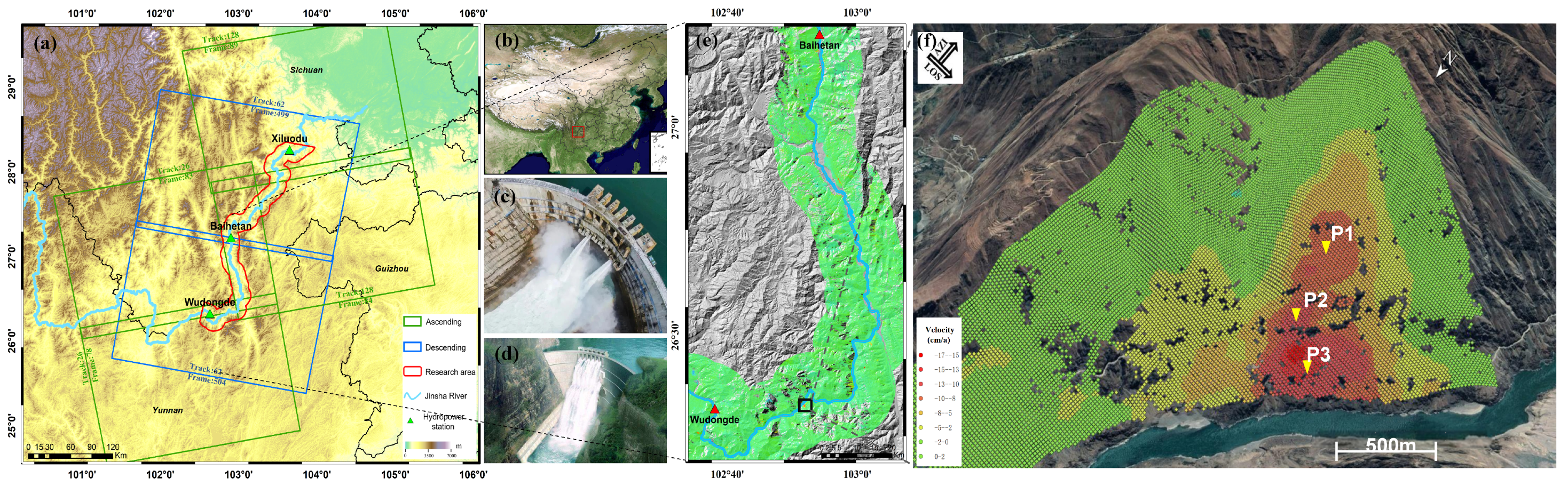
The Mianshawan landslide is strategically located at the intersection of Sichuan, Guizhou, and Yunnan provinces, upstream of the Baihetan Hydropower Station. Located approximately 101 km from the dam, this site is of critical interest due to its proximity to China’s second-largest hydropower facility. The Baihetan Dam, second only to the Three Gorges Dam in scale, is located on the downstream section of the Jinsha River, between the Wudongde and Xiluodu Hydropower Stations. The reservoir began impounding water on 6 April 2021, with water levels rising from 660 m to 817 m by 30 September 2021. The hydrological changes resulting from the dam’s operation significantly affect the stability of the landslide.

Geographically, the Mianshawan landslide is situated near 27.3 degrees north latitude and around 102.6 degrees east longitude. The geological setting of this region, characterized by well-developed stratigraphy and diverse lithology, contributes to its susceptibility to landslides. The strata in this area include formations from the Quaternary, Permian, Carboniferous, and Devonian periods, each of which has unique lithological characteristics that significantly influence the region’s landslide dynamics.

Tectonically, the region features several fault lines, notably those associated with the Zemu River and Xiaojiang, that generally have a north-south orientation. These fault zones are characterized by active tectonic movements, including left-lateral slip components, which lead to a high occurrence of geological hazards in the area, including landslides, collapses, and debris flows. The tectonic activity in these zones further increases the vulnerability of the region to such events.

Topographically, the Mianshawan landslide area features a slope gradient ranging from 26° to 35°. Prior to the reservoir impoundment, the landslide was relatively stable. However, the post-impoundment period, characterized by fluctuating water levels and prolonged water saturation, has led to significant deformation. The narrow river channel in front of the landslide poses a heightened risk of forming a barrier lake in the event of a landslide collapse. Such an occurrence could trigger catastrophic events upstream and downstream, posing considerable risks to the safe operation of the Baihetan Dam.

Deformation characteristics of the Mianshawan landslide are heavily affected by water level fluctuations. The alternating wet and dry cycles, combined with river erosion, have resulted in significant slip deformation. This displacement is further exacerbated by interactions with active fault zones, making continuous monitoring and assessment critical to mitigating potential risks. The complex interplay between these factors necessitates a comprehensive approach to landslide monitoring and management.

As shown in Figure 1, the detailed location of the Mianshawan landslide highlights its critical importance to the safety early warning of the Baihetan Hydropower Station. The complex geological setting, active fault zones, and significant deformation characteristics influenced by reservoir operations make this area a focal point for detailed geological surveys and continuous monitoring. Understanding the deformation mechanisms in this region is essential for ensuring the safety and stability of the hydropower infrastructure, thereby providing a foundation for further research and effective risk management strategies.

2.2. Processing and Analysis of the Experimental Data

2.2.1. InSAR Landslide Displacement Data

The SAR data used in this study were obtained from Sentinel-1A imagery. A total of 114 descending SAR scenes were acquired between 4 January 2019 and 2 December 2022, with a 12-day interval between acquisitions. Displacement time series for three monitoring points (P1, P2, and P3) were derived using the SBAS-InSAR technique. These data reveal significant deformation patterns, particularly at the landslide front end, where the deformation rate approaches approximately 15.6 cm/a, as shown in Figure 1f. In contrast, the rear edge exhibits minimal deformation. The distinct characteristic of this landslide is that the overall displacement is smaller than the local displacement, highlighting the importance of analyzing specific localized areas. For detailed analysis, three displacement points (P1–P3) located in the central sectors of the landslide were selected for sampling. Among them, P3, located at the front, shows a relatively higher displacement rate and magnitude, making it an ideal point for studying the landslide’s movement mechanisms.

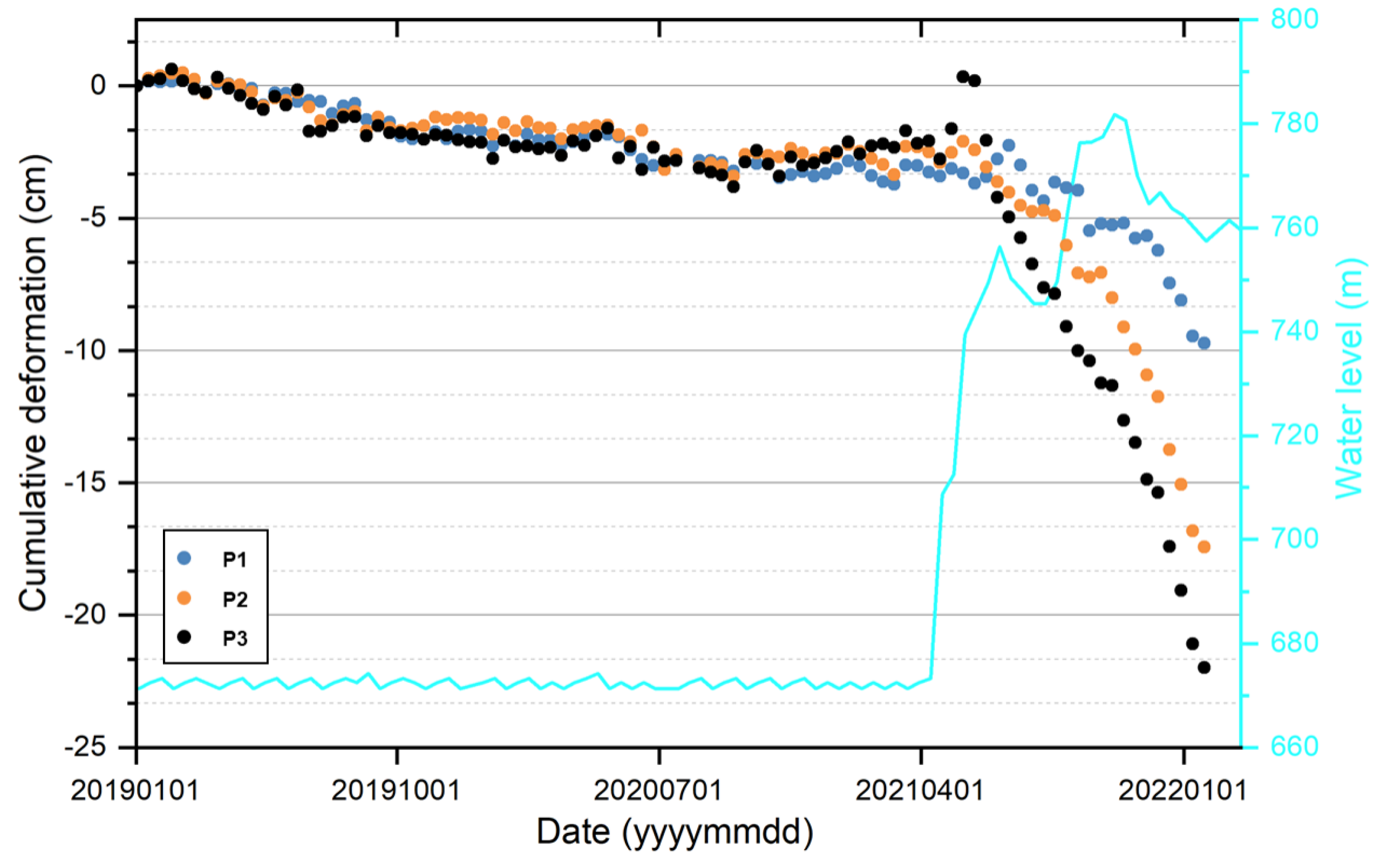
Figure 2 illustrates the deformation patterns of the Mianshawan landslide in relation to the reservoir water elevation fluctuations within the confines of the reservoir. Initially, the landslide remained relatively stable, with cumulative deformation limited to just 4 cm, and the deformation trends at all three monitoring points (P1, P2, and P3) were consistent. However, a significant shift occurred when the water level rose to 750 m. This increase triggered rapid and substantial deformation, particularly at point P3, located at the front edge of the landslide.

Within six months following the water level rise, point P3 experienced a cumulative deformation of 23 cm, indicating severe instability. In contrast, point P1, situated at the back edge, recorded a deformation of 10 cm. The pronounced deformation at point P3 can be attributed to several factors. Initially, the rapid rise in water level likely caused an increase in water absorption and subsequent expansion of the slope material, leading to an apparent uplift. This initial phase of deformation was followed by continued deformation due to the hydrostatic pressure of groundwater within the slope and an increase in soil water content.

The increased water content resulted in a reduction in soil cohesion and shear strength, especially at the foot of the slope. This reduction in mechanical properties made it difficult for the soil to adequately support the overlying material, leading to further deformation. Consequently, the deformation range of the landslide expanded, causing the slope to continue its movement. This analysis underscores the significant impact that changes in reservoir water elevation can have on the stability of the Mianshawan landslide, emphasizing the need for continuous monitoring and comprehensive analysis of environmental factors to effectively predict and mitigate potential landslide events.

In summary, the deformation patterns observed in the Mianshawan landslide following the impoundment of the reservoir highlight the complex interactions between hydrological changes and geological stability. These findings underscore the importance of ongoing observation and advanced modeling to ensure the safety of downstream infrastructures, such as the Baihetan Hydropower Station. Understanding these interactions provides critical insights for disaster management and infrastructure safety in similar geological settings.

2.2.2. Decomposed Data of Landslide Displacement Time Series and Rainfall with Reservoir Water Levels

This study also collected Level-3 daily precipitation data from the Global Precipitation Measurement (GPM) mission, covering the area with longitudes ranging from 102.85° to 102.95° and latitudes from 26.25° to 26.35°. The data have a spatial resolution of 0.1° × 0.1° and were used to explore the potential impact of precipitation on landslide deformation. The reservoir water level data were obtained based on the low backscattering signals of water bodies in SAR intensity imagery, which enabled the monitoring of water level variations and the identification of water boundaries. Due to the resolution limitations of both the DEM and SAR imagery, some inaccuracies may be present in the extracted water level data. However, the overall trend remains consistent with actual water level changes. The temporal interval of the reservoir water level data matches that of the deformation time series, with observations taken every 12 days. 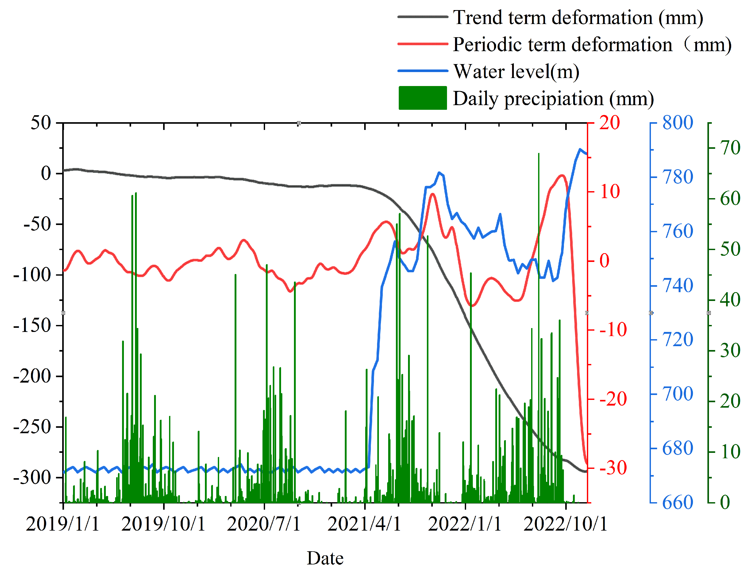For detailed information, see Figure 2. To explore the factors influencing the Mianshawan landslide, the primary Interferometric Synthetic Aperture Radar (InSAR) displacement data series at point P3 was separated into components representing trend and periodic terms using the Variational Mode Decomposition (VMD) method. Figure 3 presents these decomposed components alongside data on reservoir water elevation and daily precipitation. This decomposition provides valuable insights into how different hydrological factors influence the landslide.

The deformation represented by the trend term (black line) is closely related to the water inventory within the reservoir. Initially, before the reservoir’s impoundment, the deformation values remained minimal, indicating stable conditions. However, a substantial increase in deformation was observed post-impoundment, which strongly correlates with the rising water levels. The obvious deformation trend observed after April 2021 highlights how fluctuations in reservoir water levels influence slope stability. The rapid rise in water levels led to corresponding changes in the trend term deformation.

The periodic term deformation (red line) reflects the fluctuations in deformation that occur in response to external factors. Before the reservoir impoundment, the periodic deformation amplitude was around 5 mm and was closely linked to precipitation events. This suggests that rainfall was the primary driver of periodic deformation during this period. However, after the impoundment, the amplitude of periodic deformation increased to approximately 15 mm. This shift indicates that the influence of reservoir water level changes began to exceed that of precipitation, as evidenced by the reduced correlation between periodic deformation and rainfall events following the reservoir’s filling.

The hydrological data in the analysis provide further context for these deformations. The blue line in Figure 3 represents the water level, which shows a rapid increase from 660 m to over 780 m between April and September 2021, followed by fluctuations at this elevated level. The green bars depict daily precipitation, highlighting significant rainfall events throughout the observation period. Comparing these factors with the deformation components reveals the intricate relationship between water levels, precipitation, and landslide behavior.

In summary, this analysis demonstrates that the trend term deformation is primarily determined by the reservoir water elevation, particularly after the impoundment. The periodic term deformation, initially dominated by precipitation, becomes increasingly affected by changes in water levels post-impoundment. This dual influence highlights the complex interaction between hydrological factors and landslide dynamics, emphasizing the importance of continuous monitoring and comprehensive analysis to effectively manage and mitigate landslide risks.

2.2.3. Analysis of Landslide Deformation and Rainfall Data Using XWT and WTC

To analyze the interrelation between landslide deformation and rainfall in the Mianshawan region, XWT and WTC methods were applied. The results, as shown in Figure 4, provide a detailed understanding of the temporal relationship between these two variables. The figure consists of two subplots: subplot (a) displays the XWT, while subplot (b) illustrates the WTC analysis.

The XWT analysis between landslide deformation and rainfall is shown in Figure 4a. The color spectrum illustrates the intensity of cross-wavelet energy, where hues ranging from yellow to red denote greater energy levels. The arrows signify the phase correlation between the two time series. Arrows pointing to the right indicate similar phase characteristics, while those pointing to the left indicate opposite phase characteristics. An arrow pointing downward signifies that the second time series is leading by 90 degrees, and an arrow pointing upward indicates that the first time series is leading by 90 degrees. The WTC analysis with coherence values ranging from 0 to 1 is shown in Figure 4b. Higher values (warmer colors) suggest a significant relationship between landslide deformation and rainfall. The phase arrows in this subplot follow the same interpretation as in the XWT plot.

Identification of Significant Periods: The XWT analysis, as depicted in subplot (a), reveals significant power regions around the 128-day and 256-day periods. These regions indicate the presence of periodic components that align the deformation and rainfall data at these specific timescales.

Phase Relationship: The phase arrows predominantly point to the right within these significant power regions, indicating that the time series generally display in-phase behavior. This suggests that increases in rainfall are closely followed by corresponding increases in landslide deformation, highlighting a direct relationship between these two factors.

High Coherence Regions: In subplot (b), the WTC analysis highlights areas of high coherence, particularly around the 128-day and 256-day periods, confirming the strong correlation between rainfall and landslide deformation at these specific timescales. The coherence plot also shows variations in the correlation over time, with certain periods (e.g., around 200 to 400 days and 1000 to 1200 days) demonstrating stronger coherence. This implies that the relationship between rainfall and deformation is not constant but fluctuates, potentially due to other factors such as changes in soil saturation or groundwater levels.

The combined application of XWT and WTC methods provides a comprehensive analysis of the relationship connecting precipitation levels to landslide movement. The high coherence at specific periodicities underscores the significant influence of rainfall on landslide movements. Additionally, the phase analysis reveals the lag between rainfall events and subsequent deformation responses, which is critical for developing predictive models and early warning systems.

2.3. Predictive Model for Landslide Displacement

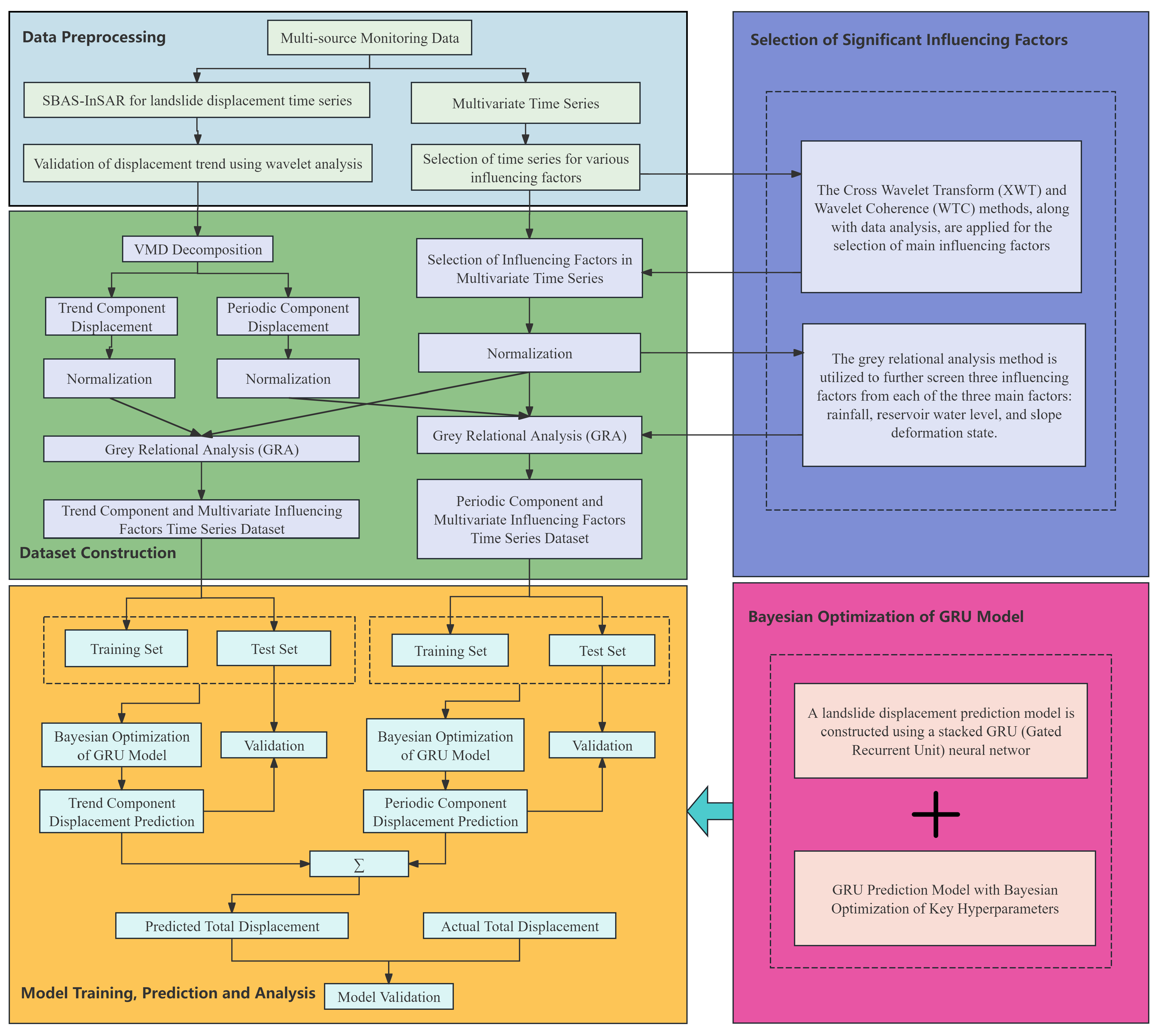
A hybrid VMD-BO-GRU method using Variational Mode Decomposition (VMD), Bayesian Optimization (BO), and Gated Recurrent Unit (GRU) is proposed for landslide displacement prediction tasks. Wavelet analysis is first applied to identify the trend term within the displacement data. Following this, the VMD method is applied to separate the aggregate displacement into its underlying trend and periodic elements. Through the application of Cross Wavelet Transform (XWT) and Wavelet Coherence (WTC) methods, supported by comprehensive data analysis, the influencing factors are determined. A broad spectrum of potential influencing factors is introduced, and Grey Relational Analysis (GRA) is employed to evaluate the relationships between each factor and both the trend and periodic components. The predictive model takes these components and the identified influencing factors as inputs. Summing the trend and periodic components yields the final cumulative displacement prediction. The methodology is illustrated in the Figure 5.

2.3.1. Displacement Involving Trend and Periodic Components

Landslide displacement is made up of two parts: trend and periodic terms. The displacement related to the trend term is mainly influenced by geological factors such as structural features, weathering, and lithology. The periodic term displacement is primarily influenced by external factors, namely precipitation and fluctuations in reservoir water levels. Therefore, the complete displacement is represented in the form of Equation (1):

$$D\left(u\right)=\alpha \left(u\right)+\beta \left(u\right)$$

(1)

Here, u represents the time variable, where $D\left(u\right)$ stands for the total displacement of the landslide, $\alpha \left(u\right)$ corresponds to the component linked to long-term trends, and $\beta \left(u\right)$ captures the oscillatory or periodic movement.

2.3.2. Variational Mode Decomposition

VMD is a flexible, non-recursive approach for breaking down signals into their inherent modes [37]. Unlike traditional methods, VMD automatically determines the number of modes and controls bandwidth to avoid modal aliasing, resulting in smoother components. The decomposition is formulated as a variational problem, aimed at minimizing the cumulative amount of projected bandwidth usage. Each mode is constrained such that their sum reconstructs the original signal, as illustrated in Equation (2):

$$\begin{array}{cc}\hfill & \underset{v_p,{\nu }_p}{min}\left\{\sum _{p=1}^P{∥{\partial }_z\left[\left(\delta \left(z\right)+{\displaystyle \frac{k}{\pi z}}\right)\ast v_p\left(z\right)\right]{\mathrm{e}}^{-k{\nu }_{p}z}∥}_2^2\right\}\hfill \\ \hfill & \mathrm{s}.\mathrm{t}.\sum _{p=1}^P{v}_p=g\hfill \end{array}$$

(2)

where $v_p\left(z\right)$ represents the mode functions, and ${\nu }_p$ are their central frequencies. ${\partial }_z$ denotes the time derivative, and $g\left(z\right)$ is the original signal.

The challenge is reformulated into a free optimization problem by incorporating a quadratic penalty term along with a Lagrangian coefficient, as expressed in Equation (3):

$$\begin{array}{cc}\hfill M(v_p,{\nu }_p,\mu )& =\beta \left\{\sum _{p=1}^{\rho }{∥{\partial }_{\zeta }\left[\left(\delta \left(z\right)+{\displaystyle \frac{k}{\pi z}}\right)\ast v_p\left(z\right)\right]∥}_2^2{\mathrm{e}}^{-k{\nu }_{p}z}\right.\hfill \\ \hfill & \left.+{∥g-\sum _{p=1}^P{v}_p∥}_2^2+\left[\mu \left(z\right),g-\sum _{p=1}^P{v}_p\right]\right\}\phantom{\sum }\hfill \end{array}$$

(3)

where $\beta$ functions as the weighting parameter, and $\mu \left(z\right)$ denotes the Lagrange multiplier. The problem is approached via the Alternating Direction Method of Multipliers (ADMM), which iteratively updates the values of $v_p$, ${\nu }_p$, and $\mu \left(z\right)$ as shown in Equations (4)–(6):

$${\widehat{v}}^{n+1}\left(\nu \right)={\displaystyle \frac{g_p^{\ast }\left(\nu \right)-{\sum }_{q\ne p}{\widehat{v}}_q\left(\nu \right)+\frac{\widehat{\mu }\left(\nu \right)}{2}}{1+2\beta (\nu -{\nu }_p)}}$$

(4)

$${\nu }_p^{n+1}\leftarrow {\displaystyle \frac{{\int }_0^{\infty }\nu {\left|{\widehat{v}}_p^{n+1}\left(\nu \right)\right|}^{2}d\nu }{{\int }_0^{\infty }{\left|{\widehat{v}}_p^{n+1}\left(\nu \right)\right|}^{2}d\nu }}$$

(5)

$${\widehat{\mu }}^{n+1}={\widehat{\mu }}^n\left(\nu \right)+\sigma (\widehat{g}\left(\nu \right)-\sum _p{\widehat{v}}_p^{n+1}\left(\nu \right))$$

(6)

where $\sigma$ refers to the tolerance for noise, and the expressions for the Fourier transforms are represented as follows: ${\widehat{v}}^{n+1}\left(\nu \right)$ corresponds to $v^{n+1}\left(z\right)$, $\widehat{g}\left(\nu \right)$ relates to $g\left(z\right)$, ${\widehat{v}}_q\left(\nu \right)$ is associated with $v_q\left(z\right)$, and $\widehat{\mu }\left(\nu \right)$ stands for $\mu \left(z\right)$.

2.3.3. Bayesian Optimization

Bayesian Optimization is a strategy for optimizing black box functions, especially those that incur high costs for evaluation or are difficult to model analytically. It constructs a probability-based model of the objective function and employs a method designed to determine the subsequent data point for analysis iteratively, aiming to find the global optimum efficiently.

The process begins by performing an evaluation of the objective function at a few initial points. These serve as the basis for building a surrogate model, often developed through the use of a Gaussian Process (GP). This model estimates the mean and variance across the search space of the function, enabling informed decisions on where to sample next. The choice of the next sampling point is guided by an acquisition function, that balances the exploration of unknown areas with the exploitation of known promising regions. Commonly used acquisition strategies include the Expected Improvement (EI) and the Upper Confidence Bound (UCB) methods.

After selecting the new sampling point, the objective function is calculated at that location, and the outcome is incorporated into the dataset to refine the surrogate model. This procedure is repeated in an iterative manner until a predefined stopping condition is satisfied. The key concepts in Bayesian Optimization include the use of a Gaussian process, which defines the surrogate model and captures the uncertainty in the objective function.

$$g\left(z\right)\sim \mathcal{GP}(\mu \left(z\right),m(z,z^{\prime }))$$

(7)

Within this framework, $\mu \left(z\right)$ represents the mean function, while $m(z,z^{\prime })$ indicates the covariance or kernel function.

The formulation of the Expected Improvement (EI) acquisition function is given by:

$${\beta }_{\mathrm{EI}}\left(z\right)=\mathbb{E}[max(0,g\left(z\right)-g\left(z^{+}\right))]$$

(8)

where $z^{+}$ is the current best point.

The Upper Confidence Bound (UCB) acquisition function can be formulated as

$${\beta }_{\mathrm{UCB}}\left(z\right)=\mu \left(z\right)+\gamma \sigma \left(z\right)$$

(9)

Here, $\gamma$ controls the balance between exploration and exploitation. The quantities $\mu \left(z\right)$ and $\sigma \left(z\right)$ correspond to the estimated mean and standard deviation, respectively, obtained from the Gaussian Process (GP) model.

2.3.4. Gate Recurrent Unit

The GRU represents an advancement in RNN architecture, designed to mitigate the challenge of gradient explosion commonly encountered in standard RNNs. As referenced in [35,41], this model integrates an innovative structure, composed of both the update gate and the reset gate, originally introduced in [42]. The reset gate plays a key role in regulating how the previous hidden state impacts the next candidate state. This process is represented by the equation below. Equation (10):

$$q_u=\sigma (W_q·[s_{u-1},y_u])$$

(10)

In this context, the Sigmoid activation is symbolized by $\sigma$, and $W_q$ stands for the weight matrix. $s_{u-1}$ designates the hidden state from the prior time step, while $y_u$ indicates the input at the current time step.

The regulation of information flow from the preceding hidden state to the current one is governed by what is termed the update gate. Mathematically, this process is articulated as:

$$v_u=\sigma (W_v·[s_{u-1},y_u])$$

(11)

where $W_v$ represents the weight matrix. By utilizing the reset gate, the prospective latent state is chosen through modifications applied to the previous hidden state combined with the current input. The formula for this computation is expressed as:

$${\tilde{s}}_u=tanh(W_s·[q_u\ast s_{u-1},y_u])$$

(12)

In this context, $W_s$ refers to the weight matrix, and * signifies element-wise multiplication.

In the final step, the update gate is merged with the candidate hidden state to choose the ultima hidden state. This is described by the Equation (13):

$$s_u=v_u\ast s_{u-1}+(1-v_u)\ast {\tilde{s}}_u$$

(13)

where $v_u$ denotes the update gate in the GRU architecture.

2.3.5. Grey Relational Analysis, GRA

Grey Relational Analysis (GRA) is used to evaluate the correlation between influencing factors. In grey system theory, the grey relational degree is used to measure whether the trends of changes among different factors are similar. The fundamental idea of GRA is to assess the similarity in geometric shapes between data sequences to determine their level of correlation. The more similar the trend between two sequences, the stronger their correlation. This method does not rely on any strict statistical assumptions and is particularly suitable for nonlinear and non-normally distributed data.

The principle is as follows: Given a reference sequence $X_0=\{x_0\left(1\right),x_0\left(2\right),\dots ,x_0\left(n\right)\}$, and multiple comparison sequences $X_i=\{x_i\left(1\right),x_i\left(2\right),\dots ,x_i\left(n\right)\}$, the data are first normalized (dimensionless processing). Common methods include the initial value method or the extreme value method to eliminate dimensional effects.

The grey relational coefficient is calculated as follows:

$${\xi }_i\left(k\right)={\displaystyle \frac{\underset{i,k}{min}{\Delta }_i\left(k\right)+\rho ·\underset{i,k}{max}{\Delta }_i\left(k\right)}{{\Delta }_i\left(k\right)+\rho ·\underset{i,k}{max}{\Delta }_i\left(k\right)}}$$

(14)

where ${\Delta }_i\left(k\right)=|x_0\left(k\right)-x_i\left(k\right)|$ is the absolute difference between the reference sequence and the comparison sequence at time k; $\rho \in [0,1]$ is the distinguishing coefficient, typically set to 0.5.

The overall grey relational degree is obtained by averaging the grey relational coefficients over all time steps:

$${\gamma }_i={\displaystyle \frac{1}{n}}\sum _{k=1}^n{\xi }_i\left(k\right)$$

(15)

A higher ${\gamma }_i$ (closer to 1) indicates that the comparison sequence $x_i$ is more strongly correlated with the reference sequence $x_0$.

2.3.6. VMD-BO-GRU Model

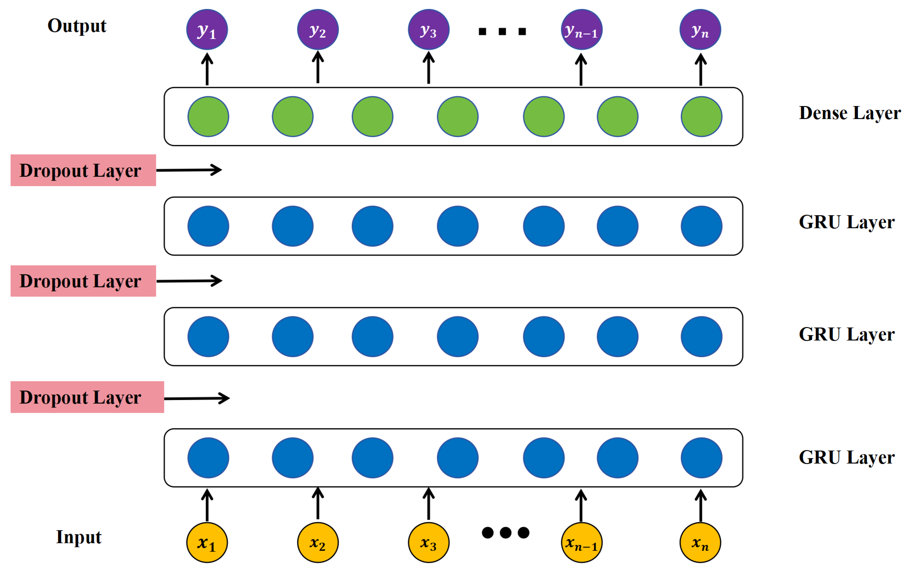
GRU excels at identifying underlying trends in time-series data. The detection technology collects deformation data in the form of a time series, $x=\{x_1,x_2,x_3,...,x_t\}$. Taking into account the advantages of GRU and its alignment with time-series results, we construct a landslide prediction model using time-series InSAR deformation data. The model employs a stacked GRU neural network composed of three GRU layers, one dense layer, and three dropout layers, as shown in Figure 6. The prediction model learns the overall trend of deformation. Ultimately, it generates the deformation prediction output $y=\{y_1,y_2,y_3,...,y_t\}$. The specific process is as outlined below:

• Model Input: Initialize weights and biases. The GRU network consists of three layers, and the dense layer features a single-layer structure. Dropout layers are used to control overfitting during the network training process. The learning rate is configured at 0.0001, with up to 1000 training iterations. Furthermore, the optimization technique utilized is the Adaptive Moment Estimation (Adam) algorithm.
• Data Normalization: To eliminate the dimension impact between data, the primary time-series InSAR dataset requires being normalized using Min–Max normalization. The original time-series InSAR data is represented as $x=\{x_1,x_2,x_3,\dots ,x_t\}$, and the corresponding normalized dataset $x^{\prime }=\{x_1^{\prime },x_2^{\prime },x_3^{\prime },\dots ,x_{t-L}^{\prime }\}$ is derived through the following process:

  $$x_i^{\prime }={\displaystyle \frac{x_i-x_{\min }}{x_{\max }-x_{\min }}}$$

  (16)
• Dataset Split: to expand the sample size of the InSAR time-series dataset, a sliding window approach is applied using a sequence length L, which produces new time-series data denoted as $x^{\prime }=\{x_1^{\prime },x_2^{\prime },\dots ,x_{t-L}^{\prime }\}$, where each $x_t^{\prime }=(x_t,x_{t+1},\dots ,x_{t+L-1})$. The resulting dataset is then partitioned into 80% for training and 20% for testing, employing the training set for subsequent model development.
• Input and Output Dimensions: The input dimensions are $(N,L,F)$, with N, L, and F indicating the sample size, time step length, and feature quantity, respectively. Finally, the output is obtained through the fully connected layer, represented as $p=\{p_1,p_2,...,p_i\}$, with the output dimension $(1,F)$.
• Inverse Data Transformation: The predicted values $\{p_1,p_2,\dots ,p_i\}$ are inversely transformed to get the final prediction result $y=\{y_1,y_2,y_3,\dots ,y_t\}$. The formula is as follows:

  $$y_n=p_n\left(x_{\max }-x_{\min }\right)+x_{\mathrm{mean}}$$

  (17)

Following data preprocessing, the Cross Wavelet Transform (XWT) and Wavelet Transform Coherence (WTC) are employed to identify key categories of influencing factors. Subsequently, Grey Relational Analysis (GRA) is utilized to select the main factors within each category. Then, training and testing sets are constructed using a sliding window method to ensure data consistency and model stability.

The proposed method employs a time-series prediction model based on GRU to predict the displacement in landslide monitoring. A multi-layer GRU structure is adopted to enable deeper feature extraction from time-series data, thereby enhancing the model’s expressive capability and prediction accuracy. The GRU model excels at capturing long-term dependencies in data and offers higher computational efficiency. Compared to traditional recurrent neural networks (RNNs), it yields improved training performance.

The model is enhanced with Bayesian Optimization (BO) to automatically tune the hyperparameters of GRU, including the number of GRU units and the dropout rate, thereby improving prediction performance. This approach eliminates the need for cumbersome manual parameter adjustment and enhances the model’s robustness and generalization capability across different datasets.

Actually, the GRU model consisted of three GRU layers with a variable number of units (ranging from 50 to 200), followed by a dropout layer (with a rate between 0.1 and 0.5) and a dense output layer. The hyperparameter bounds for Bayesian Optimization were set between 50 and 200 for the number of units and between 0.1 and 0.5 for the dropout rate, respectively. The optimization process was carried out by minimizing the RMSE on the training set to search for the above-mentioned hyperparameters. The optimal hyperparameters after iterative optimization were: ‘dropout’: 0.44, ‘units’: 191. Finally, the model was retrained using these optimal parameters, and predictions were made on the test set.

2.4. Evaluation

To assess the accuracy of the predicted outcomes, the evaluation process utilizes four key metrics. These evaluation metrics include Mean Absolute Error (MAE), Mean Absolute Percentage Error (MAPE), Root Mean Squared Error (RMSE), and the coefficient of determination ($R^2$). MAE provides an estimate of the average size of prediction errors, ignoring their direction. MAPE expresses the average error as a percentage to show how large errors are in relation to true values. RMSE measures the standard magnitude of the differences between the predicted outcomes and the actual observations, quantifying the typical deviation of predicted values from actual values.

For these metrics, lower values indicate better prediction performance. The coefficient of determination $R^2$ measures how well the predicted data fit the observed data, with values closer to 1 indicating a more accurate prediction. These metrics are defined by Equations (18), (19), (20) and (21), respectively.

$$\mathrm{MAE}={\displaystyle \frac{1}{n}}\sum _{j=1}^n|D_j-{\widehat{D}}_j|$$

(18)

$$\mathrm{MAPE}={\displaystyle \frac{1}{n}}\sum _{j=1}^n\left|{\displaystyle \frac{D_j-{\widehat{D}}_j}{D_j}}\right|\times 100\%$$

(19)

$$\mathrm{RMSE}=\sqrt{{\displaystyle \frac{{\sum }_{j=1}^n{(D_j-{\widehat{D}}_j)}^2}{n}}}$$

(20)

$$R^2=1-{\displaystyle \frac{{\sum }_{j=1}^n{(D_j-{\widehat{D}}_j)}^2}{{\sum }_{j=1}^n{(D_j-\overline{D})}^2}}$$

(21)

where $D_j$ represents the true value, ${\widehat{D}}_j$ denotes the forecasted value, and $\overline{D}$ indicates the average of the true values.

3. Experiment and Results of Landslide Displacement Prediction

3.1. Experimental Setup and Evaluation Index

The length of the dataset is from 14 January 2019 to 2 December 2022, with a time interval of one day, totaling 1429 days of data. The first 80% of the dataset is the training set, and the last 20% is the test set, after which all values were normalized. The GRU model was trained over 1000 epochs, using mini-batches of 64 samples. The optimization was performed using the Adam optimizer, with a learning rate set to 0.0001, and Mean Squared Error (MSE) was employed as the loss metric. The Bayesian Optimization process was run for 8 iterations, beginning with 3 initial random points. The comparative models include SVR, CNN, and LSTM. The model structure is based on Support Vector Regression (SVR) using a radial basis function (RBF) kernel. The input vector includes the current landslide deformation value and a set of influencing factors, and hyperparameters—including C (the regularization parameter controlling the trade-off between training error and model complexity), epsilon (the margin of tolerance where no penalty is given for errors), and gamma (the kernel coefficient determining the influence range of a single sample)—are optimized via Bayesian optimization to improve prediction accuracy. A 1D Convolutional Neural Network (CNN) was constructed with an input of time-series sequences containing landslide deformation and influencing factors. The model includes one Conv1D layer, a Flatten layer, a Dense hidden layer with dropout, and a final output layer, while key hyperparameters (number of filters and dropout rate) were optimized using Bayesian optimization. A multi-layer LSTM model with three stacked LSTM layers followed by a dropout and dense output layer was developed to predict landslide trend deformation using time-series inputs of deformation and influencing factors. Key hyperparameters, including the number of units and dropout rate, were optimized via Bayesian Optimization to enhance prediction accuracy. All the models were trained on an Intel Core i5-9300H processor, which is manufactured by Intel Corporation, based in Santa Clara, CA, USA, running at a 2.40 GHz clock speed, and coupled with an NVIDIA GeForce RTX 4090 graphics card, manufactured by NVIDIA Corporation, also based in Santa Clara, CA, USA.

3.2. Validation of Trend Component Displacement

Wavelet Transform Analysis [40] was used to detect trends in the displacement time series. By decomposing the signal into different frequency components, wavelet analysis reveals detailed insights into the signal’s behavior across various scales. Figure 7 illustrates the decomposition levels and their respective impacts on trend detection.

Level 0 represents the original displacement time series, showing a clear downward trend over time. Levels 1 to 4 show the wavelet coefficients at different decomposition levels, isolating specific frequency components of the original signal. Level 1 captures high-frequency fluctuations and noise, while Level 2 slightly smooths these fluctuations. Level 3 isolates mid-frequency components, revealing periodic patterns, and Level 4 highlights low-frequency components that emphasize long-term trends and significant displacement events.

The analysis indicates that higher decomposition levels, particularly Level 4, have larger wavelet coefficients, confirming the presence of an effective long-term tendency in the data. This suggests that the displacement is characterized by a dominant downward movement over time, which is crucial for understanding long-term displacement behavior and developing mitigation strategies.

3.3. Trend Term Displacement Prediction

Using VMD, the cumulative displacement is decomposed into two modes (IMF). In this analysis, Mode 1 is associated with the trend term, while Mode 2 is linked to the periodic term.

3.3.1. Evaluation of Correlation Degree of Influencing Factors

According to grey system principles, the grey relational coefficient [43] signifies the degree of resemblance or divergence in the progression trajectories of multiple components. If two factors show a high similarity of changes, they are considered to be related.

Choosing the relevant factors is essential for ensuring the accuracy of landslide displacement predictions. We employed XWT and WTC methods, combined with comprehensive data analysis, to identify the key external triggering factor. The principal factors influencing the deformation characteristics of landslides include rainfall and consistent variations in the water elevation of reservoirs. Additionally, the slope conditions shaped by external triggering factors generate significant repercussions for the accuracy of landslide displacement predictions.

Rainfall

Precipitation serves as the main driving force behind landslide deformation and damage. On one hand, it reshapes the slope structure by eroding the landslide surface; on the other hand, Infiltration impacts the slope by modifying its bulk density, changing the mechanical characteristics of the shifting soil, and its impact on the hydrostatic pressure is influenced [44]. The process of rainwater permeation is relatively gradual, and the effective precipitation notably influences landslide movement in the time preceding the landslide event.

Reservoir Water Elevation

The change in reservoir water elevation has two main effects on landslide deformation. Firstly, the dry-wet cycles and slope loading and unloading alter the characteristics and mechanical attributes of rock and soil. Additionally, changes in the slope’s internal seepage field influence both internal and external mechanical forces on the slope [45]. Even with the same fluctuations in reservoir water levels, the starting elevation of the reservoir near the landslide location differs, leading to different impacts on landslide deformation. Furthermore, changes in reservoir water elevation exert a delayed effect on the landslide.

Landslide Deformation State

Landslides in different deformation states have different displacement responses under the same external excitation [46]. When the landslide remains in a stable condition, even significant external forces are insufficient to trigger large-scale deformation. However, when the landslide reaches a critical threshold, minor external disturbances can disrupt the system’s equilibrium, leading to instability and triggering landslide deformation. The term “deformation state” refers to the classification of landslide displacement based on different time intervals and cumulative displacement patterns, as shown in the table. These categories include daily displacement, two-day displacement, three-day displacement, one-day prior displacement, weekly cumulative displacement, and monthly cumulative displacement. Each of these states represents different temporal scales of displacement measurement, providing a more comprehensive understanding of the landslide’s dynamic behavior.

Key Influencing Factors Were Selected Through Grey Relational Analysis (GRA)

To determine the contributing factor most relevant to landslide displacement, we systematically selected candidate factors from rainfall, reservoir water levels, and slope conditions. This selection encompasses a wide range of factors that could potentially affect the evolution of landslide displacement, as shown in

Table 1. Key Influencing Factors for Landslide Displacement.

External Inducing Factor	Impact Factor (IF)
Rainfall	Daily Precipitation
	Two-Day Cumulative Precipitation
	Three-Day Cumulative Precipitation
	Weekly Cumulative Precipitation
	Monthly Cumulative Precipitation
Reservoir Water Elevation	Reservoir Water Elevation
	Daily Reservoir Water Elevation Change
	Two-Day Reservoir Water Elevation Change
	Three-Day Reservoir Water Elevation Change
	Weekly Reservoir Water Elevation Change
	Monthly Reservoir Water Elevation Change
Landslide deformation state	Daily Displacement
	Two-Day Displacement
	Three-Day Displacement
	One-Day Prior Displacement
	Weekly Cumulative Displacement
	Monthly Cumulative Displacement

. The GRA method was then used to further refine the selection and identify the three factors most strongly correlated with displacement from these key influencing factors.

Performance Metrics Evaluation

Table 2. Association Between Trend Displacement and Key Influencing Factors.

External Inducing Factor	Impact Factor (IF)	Correlation Coefficient
Rainfall	Three-Day Cumulative Precipitation	0.471
	Weekly Cumulative Precipitation	0.485
	Monthly Cumulative Precipitation	0.502
Reservoir Water Elevation	Two-Day Reservoir Water Elevation Change	0.514
	Weekly Reservoir Water Elevation Change	0.514
	Monthly Reservoir Water Elevation Change	0.519
Landslide deformation state	Daily Displacement	0.767
	Weekly Cumulative Displacement	0.770
	Monthly Cumulative Displacement	0.797

presents the correlation between various external inducing factors and the trend components. The results indicate that the cumulative precipitation over the previous three days, week, and month yields moderate correlation coefficients of 0.471, 0.485, and 0.502, respectively. This highlights the consistent influence of precipitation on landslide displacement across different temporal scales. The two-day, weekly, and monthly variations in reservoir water elevation similarly demonstrate moderate correlations, with coefficients of 0.514, 0.514, and 0.519, respectively, underscoring the significant effect of water level elevation fluctuations in influencing landslide dynamics. Lastly, the landslide evolution indicators, specifically the displacement over the previous day, week, and month, show the highest correlation coefficients of 0.767, 0.770, and 0.797, respectively. This signifies a strong predictive relationship between prior displacement patterns and future landslide behavior.

3.3.2. Prediction of Trend-Based Displacement and Result Comparison Analysis

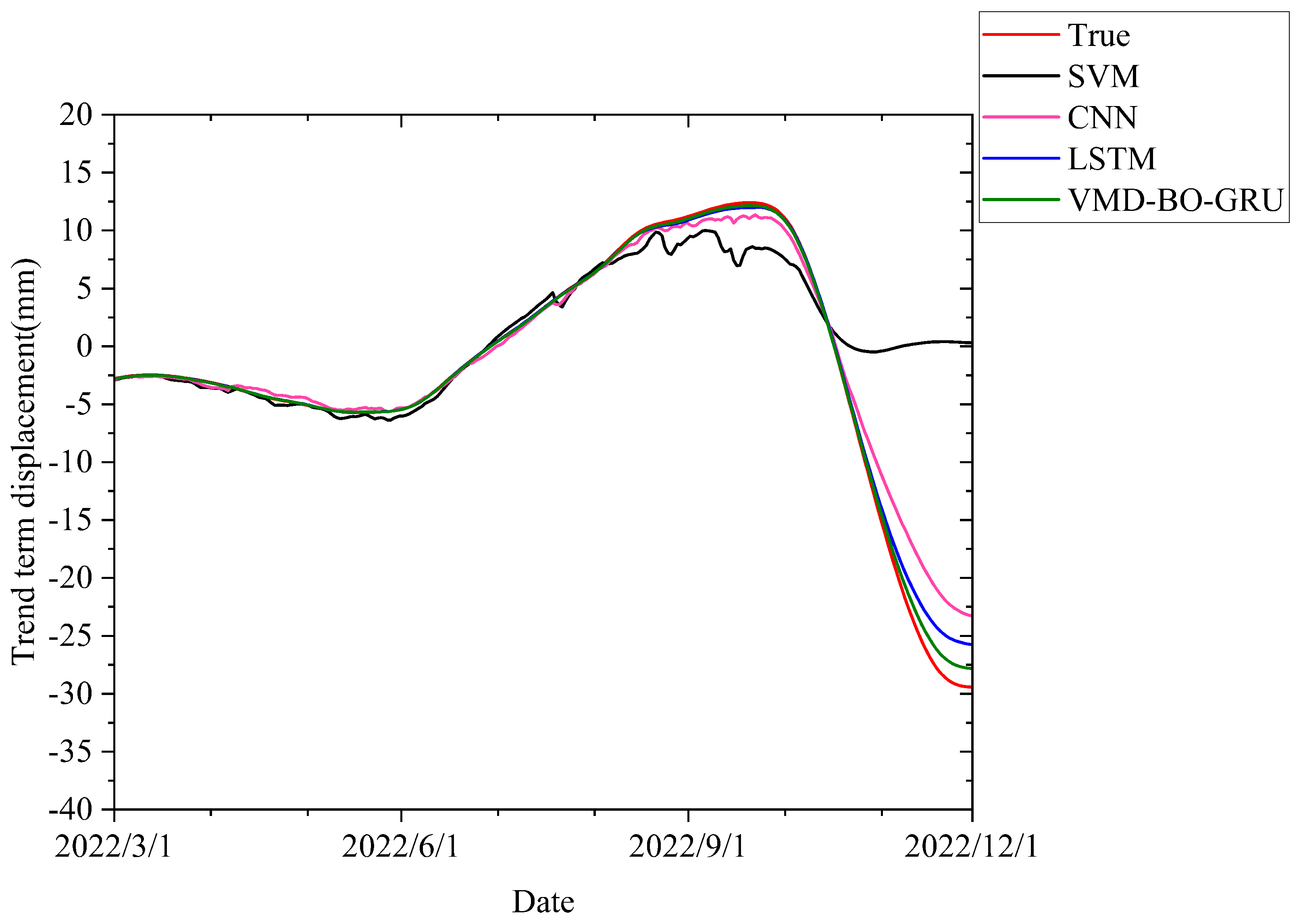
The comparative analysis of various models for trend term displacement prediction is summarized in

Table 3. Displacement evaluation index.

Model	Displacement Evaluation Index
	RMSE (mm)	MAE (mm)	MAPE	R2
SVM	111.769	93.073	34.31%	—9.583
CNN	21.345	17.722	6.67%	0.614
LSTM	10.463	8.493	3.24%	0.907
VMD-BO-GRU	2.128	2.503	1.35%	0.986

. The models compared include SVM, CNN, LSTM, and the proposed VMD-BO-GRU model. The effectiveness of these models is assessed through essential metrics such as RMSE, MAE, MAPE, and the R².

Figure 8 presents the predicted displacement trends generated by different models compared to the actual observed displacement. Our model’s prediction (green curve) closely corresponds to the actual trend (red curve) over the entire observation period. In contrast, the SVM model (black curve) exhibits significant deviations from the actual displacement trend, especially in the later phases. The CNN model (pink curve) shows a moderate improvement over SVM but still experiences notable divergence. The LSTM model (blue curve) performs reasonably well, though it does not match the accuracy of our model.

As presented in Table 3, our model demonstrates superior performance compared to alternative models in all assessed criteria. It achieved the lowest RMSE of 2.128 mm, indicating its high precision in displacement prediction. Additionally, the MAE for the model is 2.503 mm, significantly lower than that of the other models, reflecting its superior accuracy. The MAPE for this model is 1.35%, indicating that its predictions closely match the actual values on a percentage basis. Moreover, an $R^2$ value of 0.986 indicates a strong agreement between predicted and observed displacement values, reflecting the model’s excellent goodness-of-fit and predictive reliability.

These results demonstrate that our model is the most effective at predicting trend term displacement among the evaluated models. Its superior predictive performance can be attributed to its capability to capture complex temporal dependencies and long-term displacement trends, rendering it exceptionally appropriate for predicting landslide displacement.

3.4. Prediction and Analysis of Periodic Term Displacement of Landslide

The periodic displacement is derived by isolating it from the cumulative displacement after subtracting the trend component. We then conducted Grey Relational Analysis (GRA) on the influencing factors listed in Table 1 and the periodic component displacement. From each external inducing factor, the top three influencing factors with the strongest correlations were selected for predicting landslide displacement.

Table 4. Association Between Periodic Term Displacement and Key Influencing Factors.

External Inducing Factor	Impact Factor (IF)	Correlation Coefficient
Rainfal	Three-Day Cumulative Precipitation	0.458
	Weekly Cumulative Precipitation	0.488
	Monthly Cumulative Precipitation	0.530
Reservoir Water Elevation	Current Reservoir Water Elevation	0.567
	Daily Reservoir Water Elevation Change	0.540
	Monthly Reservoir Water Elevation Change	0.546
Landslide deformation state	Daily Displacement	0.818
	Weekly Cumulative Displacement	0.821
	Monthly Cumulative Displacement	0.808

illustrates the correlation coefficients linking each factor to landslide displacement.

The Prediction result of the periodic term was conducted with four models: SVM, CNN, LSTM, and our model.

3.4.1. Visual Analysis of Prediction Accuracy

Figure 9 illustrates the trend term displacement predictions over time for the different models compared to the true displacement values. The predictions of our model (the green line) closely align with the true displacement values (the red line) throughout the entire period. This close alignment is particularly notable during periods of rapid displacement changes, where other models, such as SVM (black line) and CNN (pink line), exhibit significant deviations from the true values.

The comparative analysis in Figure 9 clearly shows that our model outperforms the SVM, CNN, and LSTM models. The SVM model, with the highest RMSE and MAE, significantly underperforms, exhibiting large deviations from the true values and failing to accurately capture the displacement trends. The CNN model, although better than SVM, still shows noticeable prediction errors, particularly in capturing sudden changes in displacement. The LSTM model performs better than both SVM and CNN but still does not achieve comparable predictive accuracy.

The exceptional effectiveness of our model can be attributed to its capability to effectively capture temporal dependencies and nonlinear relationships within the displacement data. Our model’s architecture, which includes gating mechanisms, allows it to manage long-term dependencies and prevent issues such as vanishing gradients, making it especially fit for time-series prediction works like landslide displacement forecasting.

3.4.2. Performance Metrics Analysis

Table 5. Evaluation of periodic term prediction results.

Model	Displacement Evaluation Index
	RMSE (mm)	MAE (mm)	MAPE	R2
SVM	8.723	3.887	33.91%	0.293
CNN	2.048	0.991	20.92%	0.961
LSTM	1.017	0.419	5.30%	0.990
VMD-BO-GRU	0.402	0.187	2.05%	0.998

presents the displacement evaluation indices for each model. Our model outperformed the other models, exhibiting significantly better results. Specifically, with an RMSE of 0.402 mm, our model demonstrates minimal error in the average magnitude between predicted values and actual values. Similarly, our model had the lowest MAE of 0.187 mm.

The MAPE for our model was 2.05%, the lowest among all the models, showing that our model’s predictions have the smallest percentage error relative to the true values. Additionally, our model had the highest R² value of 0.998, demonstrating a high degree of alignment between the actual and the forecasted outcomes and suggesting that the model explains nearly all the variability in the data.

In summary, the impressive predictive accuracy of our proposed method is evident in its low RMSE, MAE, and MAPE values, as well as its high R² score. Moreover, the method consistently tracks the true displacement values over time. These factors collectively establish it as the most reliable model for forecasting the periodic displacement of the Mianshawan landslide. This makes our model a robust tool for landslide displacement prediction, offering crucial insights for the establishment of proactive alert mechanisms and remedial strategies.

3.5. Total Displacement Prediction

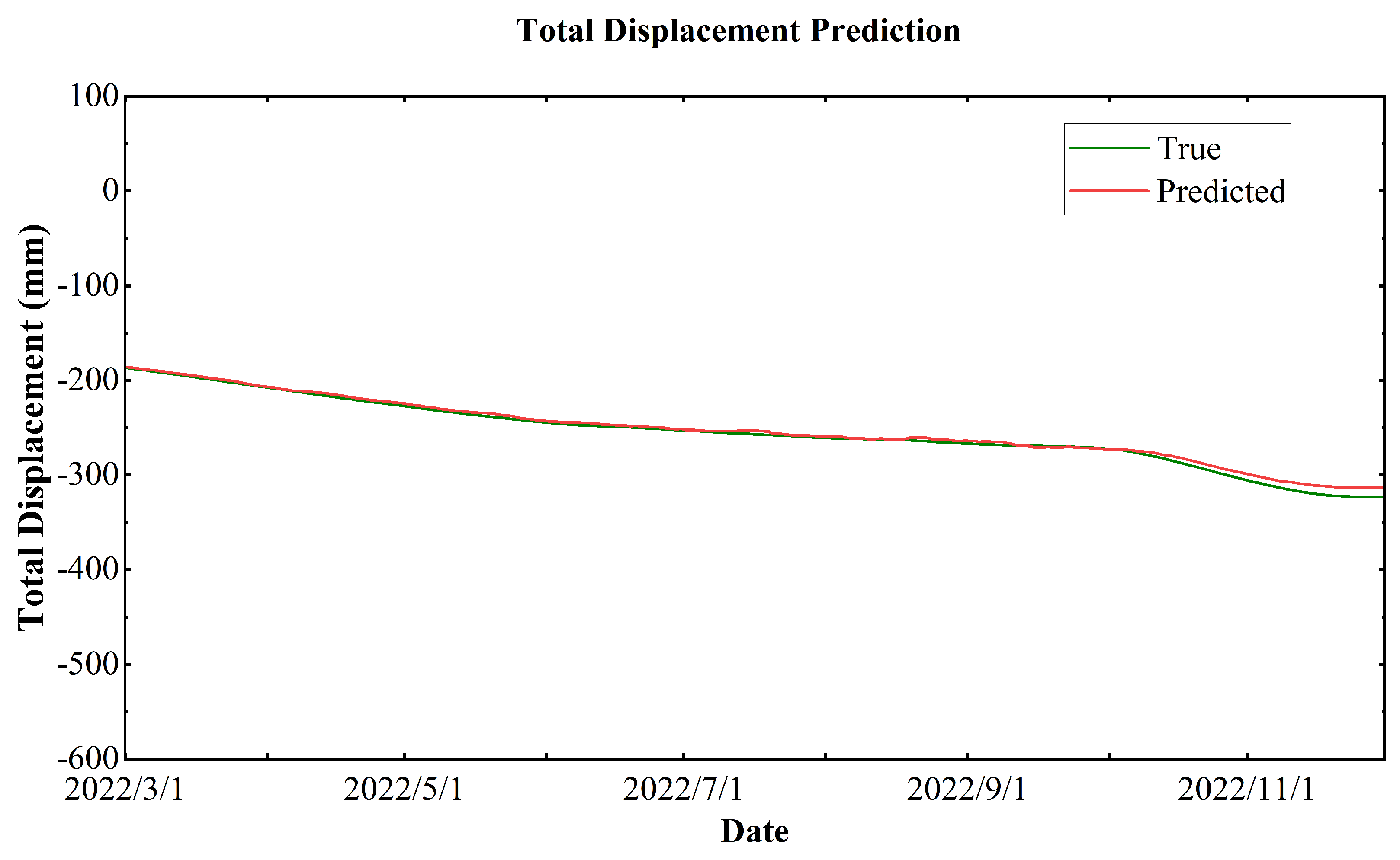
The forecast for cumulative displacement merges predictions from both trend and periodic components for a comprehensive outlook. Figure 10 displays this forecast, showcasing a comparison between the forecasted and the actual observed values.

In this figure, the red line depicts the forecasted displacement values, whereas the green line represents the actual displacement values over time. The strong correspondence between the predicted and actual values illustrates the model’s high predictive accuracy. The performance metrics for this prediction include an RMSE of 3.625 mm, a MAE of 2.683 mm, a MAPE of 0.994%, and an R² of 0.990. These metrics indicate that the VMD-BO-GRU dynamic neural network model provides highly accurate predictions of landslide displacement.

The results illustrated in Figure 10 validate the effectiveness of the VMD-BO-GRU model in capturing the dynamic evolution of slope displacement. The high precision of the constructed method shows that it can be a reliable tool for predicting landslide displacement and assisting in landslide monitoring and risk assessment.

4. Discussion

4.1. Comparison of Displacement Prediction Performance

To evaluate the effectiveness and superiority of the proposed VMD-BO-GRU model, we conducted comparative experiments on both the trend and periodic components of landslide displacement using three widely applied baseline models: Support Vector Machine (SVM) [15], Convolutional Neural Network (CNN) [33], and Long Short-Term Memory (LSTM) [31]. The experimental results are presented in Figure 8 and Table 3 for the trend component and in Figure 9 and Table 5 for the periodic component. It can be observed that our model outperforms the baseline models across all evaluation metrics for both components, demonstrating its high prediction accuracy.

4.2. Limitations and Further Considerations

Figure 9 reveals that the SVM model exhibits an opposite deformation trend from November to December 2022, likely due to its lack of memory components and limited capability to capture complex temporal dependencies and delayed responses to external variables. This highlights the limitations of static models like SVM in handling dynamic, nonlinear environments.

While the proposed model shows strong performance, there are some limitations to note. GRU may be less capable than LSTM in capturing long-term dependencies. VMD requires careful selection of decomposition parameters, and Bayesian Optimization can be computationally intensive. Despite these challenges, the combined framework still provides robust, accurate, and interpretable predictions.

4.2.1. Influence of Reservoir Regulation

The reservoir in the study area, operated by a hydropower station, undergoes frequent water level fluctuations due to seasonal impoundment and short-term release. These variations directly affect slope stability by changing the seepage conditions and toe loading. The reservoir water level is thus recognized as a key external factor in landslide deformation and is incorporated into the model.

4.2.2. Data Availability and Future Outlook

This study is based on InSAR and environmental data collected up to the end of 2022. Although the dataset captures a complete reservoir cycle and includes significant deformation phases—particularly following the rapid reservoir level rise after April 2021—it does not include data from 2023 to 2025. Incorporating this more recent period, which has seen continued deformation activity, could further enhance model validation and provide deeper insights into ongoing landslide dynamics. Future studies are encouraged to include this extended dataset.

5. Conclusions

The Mianshawan landslide region, situated in a mountainous canyon area of China, presents unique challenges for landslide displacement prediction due to its steep terrain, complex geological structures, and highly variable hydrological conditions. These factors require specialized predictive approaches to accurately model the landslide dynamics in such environments.

This paper introduces a VMD-BO-GRU model, which integrates Variational Mode Decomposition (VMD) with Gated Recurrent Units (GRU) and Bayesian Optimization (BO) for displacement prediction of landslides in high-mountain canyon areas in China. The proposed method fully leverages time-series InSAR data along with multi-source information such as geological, meteorological, and hydrological data to perform multi-level landslide displacement prediction. By introducing wavelet analysis, Variational Mode Decomposition (VMD), and influencing factor evaluation, the model’s capability to capture the complex evolution patterns of landslide deformation has been significantly enhanced. Using InSAR data from the Mianshawan landslide, comparative experiments were conducted between our approach and baseline models including SVM, CNN, and LSTM. The results demonstrate that our method achieved superior average prediction performance, with a Root Mean Squared Error (RMSE) of 0.402, Mean Absolute Error (MAE) of 0.187, Mean Absolute Percentage Error (MAPE) of 2.05%, and a coefficient of determination (R²) of 0.998. These findings indicate that, compared to traditional methods, our model delivers significant improvements in performance, offering higher prediction accuracy and greater reliability in the landslide forecasting task for the Mianshawan area.