Multi-Attitude Hybrid Network for Remote Sensing Hyperspectral Images Super-Resolution

Abstract

Benefiting from the development of deep learning, the super-resolution technology for remote sensing hyperspectral images (HSIs) has achieved impressive progress. However, due to the high coupling of complex components in remote sensing HSIs, it is challenging to achieve a complete characterization of the internal information, which in turn limits the precise reconstruction of detailed texture and spectral features. Therefore, we propose the multi-attitude hybrid network (MAHN) for extracting and characterizing information from multiple feature spaces. On the one hand, we construct the spectral hypergraph cross-attention module (SHCAM) and the spatial hypergraph self-attention module (SHSAM) based on the high and low-frequency features in the spectral and the spatial domains, respectively, which are used to capture the main structure and detail changes within the image. On the other hand, high-level semantic information in mixed pixels is parsed by spectral mixture analysis, and semantic hypergraph 3D module (SH3M) are constructed based on the abundance of each category to enhance the propagation and reconstruction of semantic information. Furthermore, to mitigate the domain discrepancies among features, we introduce a sensitive bands attention mechanism (SBAM) to enhance the cross-guidance and fusion of multi-domain features. Extensive experiments demonstrate that our method achieves optimal reconstruction results compared to other state-of-the-art algorithms while effectively reducing the computational complexity.

1. Introduction

Owing to their capacity to capture rich spectral signals from observed scenes, hyperspectral images (HSIs) can provide precise guidance for image interpretation. With advancements in hardware technology, HSIs have gradually become an important information source in remote sensing image processing. However, due to the physical limitations of imaging spectrometers, HSIs often face the challenge of low spatial resolution, which considerably constrains their potential applications, especially in tasks such as refined species classification [1,2,3] and anomaly detection [4,5,6]. Image super-resolution (SR) technology can enhance the spatial resolution of HSIs at a relatively low cost, effectively broadening the application scope.

HSI SR aims to reconstruct high-quality images with enhanced spatial resolution from existing low-resolution images. The technique pursues finer spatial details while maximally preserving spectral information. Unlike simple interpolation methods, HSI SR requires simultaneous consideration of both spatial details and spectral signals, adding to the complexity of the task. In the early stages of research, the wavelet transform (WT) [7,8], maximum a posteriori (MAP) estimation [9,10], and spectral unmixing [11,12] were prominent approaches. WT decomposes images into high- and low-frequency components, and multi-resolution analysis supporting detailed reconstruction at various scales. MAP-based methods apply statistical theories to capture correlations between reconstructed and original images, while spectral unmixing involves the decomposition and reconstruction of mixed pixels, contributing to more precise spectral representation.

With the rapid development and innovation of machine learning in image processing [13,14,15,16,17], deep learning-based methods for HSI SR have become a research hotspot in the field. Compared with traditional approaches, deep learning leverages large training data to automatically learn complex patterns within images, often demonstrating remarkable performance and generalization. The mainstream techniques can be divided into multi-image fusion and single-image super-resolution. The auxiliary images required in image fusion are usually high-resolution multispectral images (MSIs) [18,19] or panchromatic images (PANs) [20,21]. These auxiliary images provide detailed spatial information, significantly enhancing the richness of prior information. Although considerable progress has been made in this area, the approach faces two primary challenges. On one hand, the fusion of multi-modal information places higher demands on algorithms, and effectively bridging and complementing cross-modal features is the key to affecting the reconstruction results. On the other hand, the simultaneous acquisition of auxiliary images of the same observed scene necessitates additional sensors, which increases hardware costs. Additionally, fusion results are highly sensitive to registration precision between the target and auxiliary images, which limits the applicability of these methods. Therefore, some scholars have conducted research on a single HSI SR [22,23]. It is essential to account for the rich spectral information contained within the image. The calculation mode of 3D convolutions is particularly well-suited for extracting spectral features and has thus been adopted by some methods [24,25]. However, 3D convolutions also introduce high computational burdens, imposing constraints on model design. Given the evident recurrence of local features across regions and scales in remote sensing images, capturing global information is essential. Recently, Transformer has emerged as a powerful tool in various visual tasks [26,27], bringing increased attention to the exceptional performance of self-attention mechanisms. Self-attention connects pixels across global spatial locations and assigns weights, enabling an expanded receptive field without the extensive information accumulation required by conventional CNNs. It effectively reduces the distance between dependent features and establishes precise global relationships. However, the learning process of Transformer is entirely autonomous, lacking guidance from prior information, which limits learning efficiency and task orientation.

In recent years, hypergraph learning [28], as a learning mode with great potential, has been applied to image processing tasks. Hypergraph provides a more flexible and complex data representation that can connect globally interdependent feature nodes based on specific prior knowledge. This enables us to map node information into more explicit, task-oriented feature spaces, thereby guiding the learning process of the network. This transformation of feature spaces is especially advantageous for handling high-dimensional, complex data such as HSIs.

In this paper, we employ hypergraph learning as a foundational learning mode to develop a multi-attitude hybrid network (MAHN) for remote sensing HSI SR. Specifically, we apply multiple modes of transformation and re-expression to the image, enabling it to participate in network learning across various feature domains. First, we construct hypergraphs based on the high- and low-frequency features of spectral signals and spatial structures in the images to globally correlate the frequency features of each pixel and its neighborhood. For the hypergraph of frequency feature space, we design the spectral hypergraph cross-attention module (SHCAM) and spatial hypergraph self-attention module (SHSAM). The hypergraph network embedded with attention mechanisms can efficiently mine the complex correlation pattern among features and capture the long-range correlation among pixels through the representation and propagation of frequency characteristics. Furthermore, for the problem of high coupling of complex components in remote sensing HSIs, our method maps coupled spectral signals into semantic space for processing. We construct semantic hypergraphs based on the abundance of each endmember in mixed pixels to unite local scenes with strong correlations in the global scope. The similarity of the abundance matrix of each pixel reflects the similarity of the components in the corresponding observation range. After that, we construct a semantic hypergraph 3D module (SH3M) combined with 3D convolution for efficient spectral reconstruction. Finally, we design a sensitive bands attention mechanism (SBAM) to facilitate cross-domain information interaction. Specifically, the contributions of this work are as follows:

• This paper proposes a hybrid network, named MAHN, based on hypergraph learning for remote sensing HSI SR. This model can efficiently decouple and characterize complex scenes in multiple dimensions, thus realizing precise reconstruction of spatial texture and spectral signals. Extensive experiments demonstrate that our method outperforms other cutting-edge algorithms and effectively reduces the computational complexity;
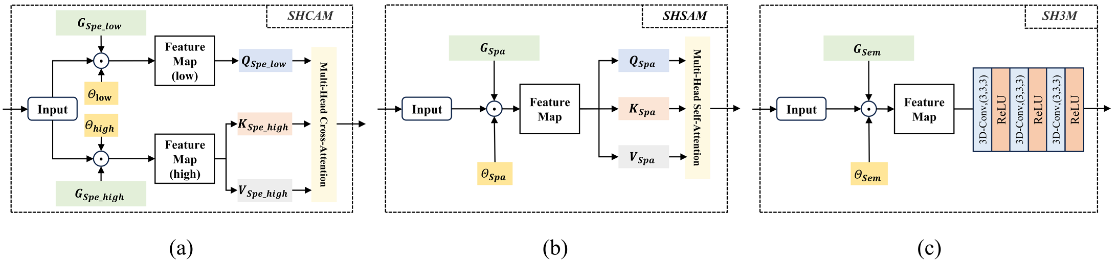
• In order to effectively extract and utilize frequency characteristics, we construct SHCAM and SHSAM based on high- and low-frequency features in spectral and spatial dimensions, respectively. Hypergraph modules with attention mechanisms achieve detailed texture and spectrum reconstruction by capturing the main structure and detail changes within the image;
• To cope with the challenge of highly coupled information in HSI, we use the semantic information in the mixed pixel to construct the relational hypergraph and design SH3M. By mapping the complex information within pixels into the semantic space, the propagation and reconstruction of a high-level semantic feature is effectively enhanced;
• To reduce domain discrepancies and enhance the compatibility among features, we design the SBAM based on the maximum entropy principle, enabling effective cross-domain interaction and fusion.

The rest of this paper is arranged as follows. Section 2 introduces the related work of multi-image fusion, single HSI SR, and hypergraph learning. In Section 3, the proposed MAHN method is introduced in detail, including the overall framework, SHCAM, SHSAM, SH3M and SBAM. Section 4 presents comprehensive experimental results with state-of-the-art methods. Section 5 discusses the effectiveness of the proposed method. Section 6 provides a summary of the study.

2. Related Works

2.1. Image Fusion for HSI SR

Due to the physical limitation, there is a trade-off between spatial and spectral resolution in imaging systems. PANs and MSIs (including RGB images) typically possess higher spatial resolution, providing richer and more detailed spatial information. Image fusion aims to combine the advantages of each to obtain HSIs with more spatial information.

Image fusion based on PANs is referred to as pan-sharpening. To better preserve the original image information, Zheng, et al. [20] designed an upsampling network based on the U-Net [29] architecture. The upsampled HSI and panchromatic images are then concatenated and fed into a fusion network with channel-spatial attention. Qu, et al. [30] propose a multi-resolution learning network that performs feature extraction across multiple scale factors, effectively reducing the learning complexity. Zhuo, et al. [31] employed multiple filters and the spectral attention mechanism to extract spatial details and spectral information separately, thereby mitigating spatial and spectral distortion. To cope with SR tasks at an arbitrary scale, He, et al. [32] proposed an arbitrary upsampling framework based on variable sub-pixel convolution. This method eliminates the reliance on fixed-scale training samples and greatly improves the application potential of pan-sharpening technology.

Since MSIs also carry spectral information, they offer greater flexibility when fused with HSIs. To better address SR tasks with unknown degradation, Zhang, et al. [33] proposed a two-stage network. This network reconstructs the image in a coarse-to-fine manner while simultaneously estimating the degradation process, thereby improving generalization ability. Considering the correlation between samples, Guo, et al. [34] employed an external attention mechanism to learn better feature representations across different samples. Hong, et al. [35] proposed a sub-pixel level fusion framework that considers the intrinsic differences between MSI and HSI, utilizing their inherent properties for feature fusion. Zheng, et al. [36] proposed an unsupervised model to address the fusion task under the unknown conditions of the point spread function and spectral response function. Considering the non-overlapping spectral ranges between MSI and HSI, Sun, et al. [37] extended the overlapping-nonoverlapping relationship from HSI to the fused image, enhancing the spectral fidelity of the result.

2.2. Single HSI SR

Single HSI SR can remove the limitation of data and reduce the technical cost. Due to the lack of supplementary information from auxiliary images, the extraction of internal features within the image becomes a key factor affecting performance.

Unlike natural images, HSI processing requires extra attention to spectral information. Benefitting from the special calculation mode, 3D convolution performs excellently in extracting spectral features. Mei, et al. [38] and Li, et al. [39] replaced 2D convolution in the MSI SR framework [40,41] with 3D convolution, marking early attempts in this direction. Li, et al. [42] combined 3D convolution with generative adversarial networks and introduced band attention to capture band dependence. In order to balance the extraction of spatial/spectral information and reduce the overhead, Li, et al. [24,25] proposed the idea of cross-using 2D/3D convolution. The dual-channel network designed by Wang, et al. [43] can improve learning ability through information sharing. Chen, et al. [44] proposed a multi-branch network aimed at multi-scale representation of internal features, which alleviates the computational burden caused by 3D convolutions. Liu, et al. [45] designed a dual-domain network based on 2D/3D convolution to enhance spatial-spectral consistency. Features in remote sensing images exhibit cross-regional recurrence, making global information capturing particularly important. To achieve a larger receptive field, CNNs often need to provide larger convolutional kernels and deeper architectures, which limits the flexibility of network design. Transformer can more directly establish global relationships based on self-attention mechanisms. Liu, et al. [46] designed a dual-branch network that utilizes Transformer and 3D convolution to extract global and local information, respectively. Wu, et al. [47] embed 3D convolution into Transformer to enhance information extraction capability. Hu, et al. [48] proposed a method that transforms the image into the abundance domain, also incorporating the attention mechanism.

In addition to the aforementioned learning networks, there are also some strategies favored by scholars. Transfer learning is an effective approach to alleviate data scarcity. Yuan, et al. [49] applied transfer learning to map LR/HR relationships in natural images to HSIs, which reduced the dependency on training data. Cheng, et al. [50] leveraged large-scale nonhomologous datasets to improve model generalizability. Due to the advantages of the diffusion model in handling generative tasks, some scholars have also introduced it into HSI SR [51,52]. The high dimensionality and redundancy of HSI data increase the difficulty of feature extraction, and band grouping is an effective strategy. Jiang, et al. [53] group the bands in HSI and decompose the complex task into multiple sub-tasks, thereby reducing the learning difficulty of the network. Subsequently, Wang, et al. [54] proposed an integration module to leverage the correlation between neighboring bands for information supplementation. Related studies were also conducted in the work of Wang, et al. [55] and Zhao, et al. [56]. When employing this strategy, the problem of information loss in grouping and information redundancy in fusion should be paid more attention to.

2.3. Hypergraph Learning

Hypergraph learning is a machine learning method based on hypergraph structure, which further improves the ability of graph learning to deal with complex data. A hypergraph is a special graph structure composed of hyperedges and nodes. Compared with the ordinary graph, each hyperedge can connect multiple feature nodes, indicating the correlation between nodes in one or more aspects. Hypergraphs are capable of mapping the structural and semantic relationships within the data to another feature space, thereby improving the efficiency of information aggregation and interpretation.

Feng, et al. [28] proposed the hypergraph neural network (HGNN) for representation learning. The feature update formula is as follows:

$$\mathit{Y}={\mathit{D}}_{\mathit{v}}^{-1/2}\mathit{H}\mathit{W}{\mathit{D}}_{\mathit{e}}^{-1}{\mathit{H}}^T{\mathit{D}}_{\mathit{v}}^{-1/2}\mathit{X}\mathit{\theta },$$

(1)

where $\mathit{H}$ represents the hypergraph, ${\mathit{D}}_{\mathit{e}}$ and ${\mathit{D}}_{\mathit{v}}$ denote the diagonal matrices of the edge degrees and the vertex degrees, respectively, $\mathit{W}$ is initialized as an identity matrix, which means equal weights for all hyperedges, $\mathit{\theta }$ represents the update parameters in the network. For more details about the HGNN, please refer to [28]. The potential of hypergraph learning has been demonstrated in various fields [57,58].

The excellent properties exhibited by hypergraphs make them highly suitable for handling complex data. Due to the lower spatial resolution, the information in remote sensing HSIs is highly coupled and the components are mixed, making feature extraction more challenging. Hypergraphs are capable of mining higher-order relationships from different feature dimensions, establishing global associations. In this paper, we achieve more precise feature extraction and reconstruction by applying hypergraph learning on both frequency features and semantic information.

3. Materials and Methods

In this section, we provide a detailed description and interpretation of the proposed multi-attitude hybrid network (MAHN). First, we introduce the complete model architecture and reconstruction process. Following this, we present each component of the model individually, including the spectral hypergraph cross-attention module (SHCAM), spatial hypergraph self-attention module (SHSAM), semantic hypergraph 3D module (SH3M), and the sensitive bands attention mechanism (SBAM).

3.1. Overall Framework

The proposed MAHN aims to reconstruct high-resolution (HR) HSI from low-resolution (LR) HSI, i.e.,

$${\mathit{I}}_{SR}=F_{MAHN}\left({\mathit{I}}_{LR}\right)\in {\mathbb{R}}^{sH\times sW\times C},$$

(2)

where $H$, $W$, $C$ represent the height, width, and number of bands of the LR image, respectively, and $s$ denotes the scaling factor.

The MAHN consists of four branches: the Spectral-Net, Spatial-Net, Semantic-Net, and Res-Net. Additionally, the SBAM is designed to facilitate cross-domain information interaction and fusion. The structure is shown in Figure 1.

The Spectral-Net is composed of cascaded SHCAM. First, hypergraph operators are constructed based on low- and high-frequency features in the spectrum, represented as ${\mathit{G}}_{Spe\_low}$ and ${\mathit{G}}_{Spe\_high}$, respectively. The outputs after the first module and the $n$-th module are represented as follows:

$${\mathit{I}}_{SHCAM}^1=f_{SHCAM}^1\left({\mathit{I}}_{LR},{\mathit{G}}_{Spe\_low},{\mathit{G}}_{Spe\_high}\right),$$

(3)

$${\mathit{I}}_{SHCAM}^n=f_{SHCAM}^n\left({\mathit{I}}_{SHCAM}^{n-1},{\mathit{G}}_{Spe\_low},{\mathit{G}}_{Spe\_high}\right),$$

(4)

where $f_{SHCAM}^n$ represents the function of the $n$-th SHCAM.

Similarly, the Spatial-Net consists of a series of cascaded SHSAMs. The hypergraph operators are constructed based on low- and high-frequency features in spatial textures, denoted as ${\mathit{G}}_{Spa\_low}$ and ${\mathit{G}}_{Spa\_high}$, respectively. The two are summed to obtain the final spatial hypergraph operator denoted as ${\mathit{G}}_{Spa}$. The outputs of the first module and the $n$-th module are denoted as

$${\mathit{I}}_{SHSAM}^1=f_{SHSAM}^1\left({\mathit{I}}_{LR},{\mathit{G}}_{Spa}\right),$$

(5)

$${\mathit{I}}_{SHSAM}^n=f_{SHSAM}^n\left({\mathit{I}}_{SHSAM}^{n-1},{\mathit{G}}_{Spa}\right),$$

(6)

where $f_{SHSAM}^n$ represents the function of the $n$-th SHSAM.

The Semantic-Net is composed of cascaded SH3Ms. The unmixing algorithm is used to extract the abundances of endmembers in the mixed pixels, and based on this, the semantic hypergraph operator, denoted as ${\mathit{G}}_{Sem}$, is constructed. The outputs after the first module and the $n$-th module are represented as

$${\mathit{I}}_{SH3M}^1=f_{SH3M}^1\left({\mathit{I}}_{LR},{\mathit{G}}_{Sem}\right),$$

(7)

$${\mathit{I}}_{SH3M}^n=f_{SH3M}^n\left({\mathit{I}}_{SH3M}^{n-1},{\mathit{G}}_{Sem}\right),$$

(8)

where $f_{SH3M}^n$ represents the function of the $n$-th SH3M.

Additionally, for the ${\mathit{I}}_{SHCAM}^1$, ${\mathit{I}}_{SHSAM}^1$, and ${\mathit{I}}_{SH3M}^1$ in the above three branches, the sensitive bands are selected based on the maximum entropy principle. These serve as weight layers from different domains and are fed into the Res-Net, with the weights represented as

$$\mathit{w}=f_{BS}\left({\mathit{I}}_{SHCAM}^1,{\mathit{I}}_{SHSAM}^1,{\mathit{I}}_{SH3M}^1\right),$$

(9)

where $f_{BS}$ represents the function of band selection. The output of the third and last module in the Res-Net is

$${\mathit{I}}_{Res}^3=f_{Res}^3\left({\mathit{I}}_{Res}^2+{\mathit{I}}_{Res}^2\ast \mathit{w}\right),$$

(10)

$${\mathit{I}}_{Res}^n=f_{Res}^n\left({\mathit{I}}_{Res}^{n-1}\right).$$

(11)

Finally, the outputs of the four branches are added and fed into the reconstruction module (RM), i.e.,

$${\mathit{I}}_{RM}=f_{RM}\left({\mathit{I}}_{SHCAM}^n+{\mathit{I}}_{SHSAM}^n+{\mathit{I}}_{SH3M}^n+{\mathit{I}}_{Res}^n\right),$$

(12)

$${\mathit{I}}_{SR}=f_{Conv}\left({\mathit{I}}_{RM}+BIC\left({\mathit{I}}_{LR}\right)\right)\in {\mathbb{R}}^{sH\times sW\times C}.$$

(13)

In MAHN, n is set to 6.

3.2. SHCAM

In the HSI SR task, accurately extracting and processing the low- and high-frequency characteristics of spectral signals is conducive to improving the spectral quality of the reconstructed image. Low-frequency features better represent the global structure and trend of the spectrum, while high-frequency features are helpful in observing subtle spectral differences between similar targets. Therefore, we propose a spectral feature extraction module, named SHCAM, to better represent and utilize spectral information, as shown in Figure 2a.

We first apply 1D-WT to all spectra, obtaining the approximation coefficients (cA) and detail coefficients (cD):

$$\mathit{c}\mathit{A},\mathit{c}\mathit{D}={WT}_{1-D}\left({\mathit{I}}_{LR}\right)\in {\mathbb{R}}^{H\times W\times {\displaystyle \frac{c}{2}}}.$$

(14)

After that, we construct hypergraphs based on the similarity of the low- and high-frequency characteristics between spectra, respectively. The nodes in the hypergraphs correspond to the $\mathit{c}\mathit{A}$ or $\mathit{c}\mathit{D}$ of each spectrum, and the hyperedges indicate the similarity between nodes. The higher the similarity, the higher the weight assigned to the node. Specifically, each hyperedge contains ten nodes selected through the k-nearest neighbor (KNN) algorithm based on Euclidean distance, and the weights of the nodes are obtained using a negative exponential function. The process of constructing the hypergraph can be represented as follows:

$${\mathit{H}}_{Spe\_low},{\mathit{H}}_{Spe\_high}=f_{HC}\left(\mathit{c}\mathit{A},\mathit{c}\mathit{D}\right)\in {\mathbb{R}}^{N\times N},$$

(15)

where $f_{HC}$ represents the complete function of hypergraph construction, and $N=HW$ represents the number of nodes. After that, the hypergraph is converted to a hypergraph operator, and the process is formulated as

$${\mathit{G}}_{Spe\_low}={\mathit{D}}_{\mathit{v}}^{-1/2}{\mathit{H}}_{Spe\_low}\mathit{W}{\mathit{D}}_{\mathit{e}}^{-1}{{\mathit{H}}_{Spe\_low}}^T{\mathit{D}}_{\mathit{v}}^{-1/2},$$

(16)

$${\mathit{G}}_{Spe\_high}={\mathit{D}}_{\mathit{v}}^{-1/2}{\mathit{H}}_{Spe\_high}\mathit{W}{\mathit{D}}_{\mathit{e}}^{-1}{{\mathit{H}}_{Spe\_high}}^T{\mathit{D}}_{\mathit{v}}^{-1/2}.$$

(17)

The process of feature updating is formulated as

$${\mathit{I}}_{Spe\_low}^n={\mathit{G}}_{Spe\_low}·{\mathit{I}}_{SHCAM}^{n-1}·{\mathit{\theta }}_{low},$$

(18)

$${\mathit{I}}_{Spe\_high}^n={\mathit{G}}_{Spe\_high}·{\mathit{I}}_{SHCAM}^{n-1}·{\mathit{\theta }}_{high}.$$

(19)

Afterward, a cross-attention algorithm is applied to better exploit the dependencies between the high and low-frequency features. Specifically, the Query (Q) comes from the low-frequency features, while the Key (K) and Value (V) come from the high-frequency features, denoted as ${\mathit{Q}}_{Spe\_low}$, ${\mathit{K}}_{Spe\_high}$ and ${\mathit{V}}_{Spe\_high}$, respectively. The features are then fed into the multi-head cross-attention (MHCA) mechanism for fusion, which is

$${\mathit{I}}_{SHCAM}^n=MHCA\left({\mathit{Q}}_{Spe\_low},{\mathit{K}}_{Spe\_high},{\mathit{V}}_{Spe\_high}\right).$$

(20)

In summary, the complete feature extraction in SHCAM can be expressed as follows:

$${\mathit{I}}_{SHCAM}^n=f_{SHCAM}^n\left({\mathit{I}}_{SHCAM}^{n-1},{\mathit{G}}_{Spe\_low},{\mathit{G}}_{Spe\_high}\right).$$

(21)

In this module, the frequency characteristics of each signal node are considered, which effectively enhances the fidelity of the reconstructed spectra. In addition, the target has obvious cross-regional recurrence, and the hypergraph represents the dependency between nodes in the global scope. Hypergraph learning can capture the long-range correlation between pixels, thus enhancing the richness and breadth of the learning process.

3.3. SHSAM

In addition to spectral information, capturing and utilizing spatial information is equally important for the SR task. Low-frequency signals in the spatial domain represent features that change slowly. This part exhibits smooth variations and typically contains the main structural information of the observed scene, such as the background and brightness distribution. High-frequency signals represent rapidly changing features, such as the edge and texture of the target. Therefore, we construct a spatial feature extraction module, named SHSAM, to achieve accurate reconstruction of structure and detail texture, as shown in Figure 2b.

HSIs typically consist of hundreds of bands, containing a significant amount of redundant information, and the quality of each band is quite different. To simplify the processing and reduce computational cost, principal component analysis (PCA) is applied for dimensionality reduction. Then, the 2D-WT is performed on the reduced-dimensional image, which is

$$\mathit{L}\mathit{L},\left(\mathit{L}\mathit{H},\mathit{H}\mathit{L},\mathit{H}\mathit{H}\right)={WT}_{2-D}\left(PCA\left({\mathit{I}}_{LR}\right)\right)\in {\mathbb{R}}^{{\displaystyle \frac{H}{2}}\times {\displaystyle \frac{W}{2}}\times k},$$

(22)

where $\mathit{L}\mathit{L}$, $\mathit{L}\mathit{H}$, $\mathit{H}\mathit{L}$ and $\mathit{H}\mathit{H}$ represent the low-frequency components and the high-frequency components from the horizontal, vertical, and diagonal directions, respectively, and $k$ represents the number of dimensions retained after PCA. After that, we perform bicubic interpolation on frequency maps, expanding the extracted frequency features, and then construct the hypergraph separately. Given the strong correlation between the main structures and fine textures, we combine the two to participate in network learning,

$${\mathit{H}}_{Spa\_low},{\mathit{H}}_{Spa\_high}=f_{HC}\left(\mathit{L}\mathit{L},(\mathit{L}\mathit{H},\mathit{H}\mathit{L},\mathit{H}\mathit{H})\right)\in {\mathbb{R}}^{N\times N},$$

(23)

$${\mathit{H}}_{Spa}={\mathit{H}}_{Spa\_low}+{\mathit{H}}_{Spa\_high},$$

(24)

where ${\mathit{H}}_{Spa}$ is the spatial hypergraph that is ultimately used for the model, then convert ${\mathit{H}}_{Spa}$ into a hypergraph operator, i.e.,

$${\mathit{G}}_{Spa}={\mathit{D}}_{\mathit{v}}^{-1/2}{\mathit{H}}_{Spa}\mathit{W}{\mathit{D}}_{\mathit{e}}^{-1}{{\mathit{H}}_{Spa}}^T{\mathit{D}}_{\mathit{v}}^{-1/2}.$$

(25)

The process of feature updating is formulated as follows:

$${\mathit{I}}_{Spa}^n={\mathit{G}}_{Spa}·{\mathit{I}}_{SHSAM}^{n-1}·{\mathit{\theta }}_{Spa}.$$

(26)

After that, in order to better activate global information and expand the receptive field of each pixel, the features enhanced by hypergraph learning will be fed into a multi-head self-attention mechanism (MHSA), which is

$${\mathit{I}}_{SHSAM}^n=MHSA\left({\mathit{Q}}_{Spa},{\mathit{K}}_{Spa},{\mathit{V}}_{Spa}\right).$$

(27)

In summary, the complete feature extraction in SHSAM can be expressed as

$${\mathit{I}}_{SHSAM}^n=f_{SHSAM}^n\left({\mathit{I}}_{SHSAM}^{n-1},{\mathit{G}}_{Spa}\right).$$

(28)

Hypergraph learning based on the main structure and detailed texture can effectively utilize the similar features in the image, enabling mutual enhancement between feature points and precise reconstruction of spatial information.

3.4. SH3M

In HSIs, a pixel often corresponds to a relatively large observation area, which means the image contains a significant number of mixed pixels. Different targets typically exhibit complex interlacing and overlapping patterns, and this uneven distribution and multi-class coupling affect the expression of their respective spatial, spectral, and frequency information. Decoupling the information of mixed pixels allows for more precise feature decomposition and reconstruction, reducing the interference of multidimensional information in complex environments. Therefore, we propose a semantic learning module, named SH3M, to achieve high-quality semantic information extraction, as shown in Figure 2c.

We utilize the non-negative matrix factorization (NMF) algorithm based on gradient descent to estimate the endmember matrix and the abundance matrix. The basic form can be expressed as the following:

$$\mathit{X}\approx \mathit{A}\mathit{E},$$

(29)

where $\mathit{X}\in {\mathbb{R}}^{N\times C}$ is the original hyperspectral data, $\mathit{A}\in {\mathbb{R}}^{N\times q}$ is the abundance matrix, $\mathit{E}\in {\mathbb{R}}^{q\times C}$ represents the endmember matrix, and $q$ represents the number of endmembers. The objective function of NMF is

$$\underset{\mathit{A},\mathit{E}}{\mathit{min}}{‖\mathit{X}-\mathit{A}\mathit{E}‖}_F^2=\underset{\mathit{A},\mathit{E}}{\mathit{min}}\sum _{i=1}^N\sum _{j=1}^C{\left({\mathit{X}}_{ij}-{\left(\mathit{A}\mathit{E}\right)}_{ij}\right)}^2,$$

(30)

where ${‖·‖}_F^2$ represents the Frobenius norm. Additionally, the obtained abundance matrix and endmember matrix must satisfy the non-negativity constraint and the sum-to-one constraint, i.e.,

$$\mathit{A}\ge 0,\mathit{E}\ge 0,and\sum _{j=1}^q{\mathit{A}}_{ij}=1,\forall i\in \left\{1,\dots ,N\right\}.$$

(31)

Subsequently, the hypergraph is constructed based on the abundance matrix to map the original spectral information into a high-level semantic space, which is

$${\mathit{H}}_{Sem}=f_{HC}\left(\mathit{A}\right)\in {\mathbb{R}}^{N\times N},$$

(32)

$${\mathit{G}}_{Sem}={\mathit{D}}_{\mathit{v}}^{-1/2}{\mathit{H}}_{Sem}\mathit{W}{\mathit{D}}_{\mathit{e}}^{-1}{{\mathit{H}}_{Sem}}^T{\mathit{D}}_{\mathit{v}}^{-1/2},$$

(33)

where ${\mathit{H}}_{Sem}$ and ${\mathit{G}}_{Sem}$ represent a hypergraph and the hypergraph operator containing semantic information, respectively. The process of feature updating is formulated as

$${\mathit{I}}_{Sem}^n={\mathit{G}}_{Sem}·{\mathit{I}}_{SH3M}^{n-1}·{\mathit{\theta }}_{Sem}.$$

(34)

To better extract spectral features, we employ 3D convolution in the subsequent learning process, which can be formulated as

$${\mathit{I}}_{SH3M}^n=f_{3D-Conv}\left({\mathit{I}}_{Sem}^n\right).$$

(35)

In summary, the complete feature extraction in SH3M can be expressed as

$${\mathit{I}}_{SH3M}^n=f_{SH3M}^n\left({\mathit{I}}_{SH3M}^{n-1},{\mathit{G}}_{Sem}\right).$$

(36)

One of the advantages of hypergraph learning is its ability to support cross-pixel collaborative optimization among nodes. By clustering pixels with similar abundance distributions into the same hyperedge, the model can consider cooperative relationships between different pixels during optimization. Mapping highly coupled information into a more explicit high-level semantic space effectively reduces the difficulty of information propagation, thereby facilitating more precise detail reconstruction.

3.5. SBAM

The three modules described above independently extract spectral, spatial, and high-level semantic information, providing comprehensive guidance for the reconstruction. However, domain discrepancies exist among the features extracted by each module, and independent learning paths often lead to compatibility issues with the features. In this section, we introduce the SBAM for cross-domain information fusion.

Each band of HSI carries information of different intensity and quality. In SBAM, the most informative band is selected from the three branches using the maximum entropy principle, which is considered to be the sensitive band carrying the most specific features. First, we perform pixel value statistics for each band of features in the spectral, spatial, and semantic branches, estimating the pixel value probability distribution $P\left(x\right)$. Then, the entropy of each band is calculated, which is expressed as follows:

$$H\left({\mathit{X}}_i\right)=-\sum _{x\in X_i}P\left(x\right)\mathit{log}P\left(x\right),$$

(37)

where ${\mathit{X}}_i$ is the set of pixel values in the $i$-th band. The band ${\mathit{X}}_{max}$ with the highest entropy is selected as the sensitive band. After that, the sensitive bands from the three branches are applied collectively to the residual branch as the weight layer, which is formulated as

$$\mathit{w}=Sigmoid\left({\mathit{X}}_{max}^{Spe}+{\mathit{X}}_{max}^{Spa}+{\mathit{X}}_{max}^{Sem}\right),$$

(38)

$${\mathit{I}}_{Res}^3=f_{Res}^3\left({\mathit{I}}_{Res}^2+{\mathit{I}}_{Res}^2\ast \mathit{w}\right).$$

(39)

The weights reflect the importance of each pixel in different feature spaces. Before the feature map is fed into the third residual block, it will be guided and adjusted by information from other branches. The intervention of the sensitive band attention dynamically adjusts the weight of each feature during fusion, thereby more accurately guiding the interaction between spectral, spatial, and high-level semantic information. This approach ensures the collaborative optimization of different feature domains, ultimately improving the reconstruction performance.

4. Results

This section presents an experimental analysis of MAHN to validate the effectiveness of the proposed method. Specifically, MAHN will be compared against representative works in the field from recent years in terms of metrics and visual quality.

4.1. Implementation Details

Datasets we selected for this experiment include the MDAS dataset, the Houston dataset, and the Pavia Centre dataset. The input LR HSIs for both training and testing were generated by bicubic downsampling. The SR reconstruction tasks target scaling factors of $2\times$, $3\times$, and $4\times$, with input images sized at $32\times 32$. The joint loss function consists of L1 loss, spectrum loss, and gradient loss, weighted at 1:0.3:0.1, respectively. The Adam optimizer (${\beta }_1=0.9$ and ${\beta }_2=0.999$) was employed for parameter updates, and the initial learning rate was set to 0.0001. The full training process included 40K iterations, with the learning rate halved after 30K iterations. Metrics used for quantitative evaluation of reconstructed image quality included peak signal-to-noise ratio (PSNR), structural similarity (SSIM) [59], spectral angle mapper (SAM) [60], and the Erreur Relative Globale Adimensionnelle de Synthèse (ERGAS) [61]. All the training and testing processes of this experiment are done in the same environment. Our method is implemented on the PyTorch 1.11.0 framework with an NVIDIA GeForce GTX 3090 GPU.

The MAHN will be compared with several representative methods in recent years. Specifically, these methods include 3D-FCNN [38], GDRRN [39], SSPSR [53], MCNet [24], ERCSR [25], GELIN [54], SRDNet [45], and MSSR [44]. Among them, in addition to the early-stage classical models, SSPSR and GELIN stand out as prominent works in band grouping strategies, while MCNet, ERCSR, SRDNet, and MSSR represent seminal efforts in exploring attention mechanisms and 3D convolutions. These works largely epitomize the developmental trajectory of this field and offer significant guidance for our methodology. The quality of reconstructed images will be evaluated using four objective metrics, visualization results, error heat maps, and the mean spectral difference curves.

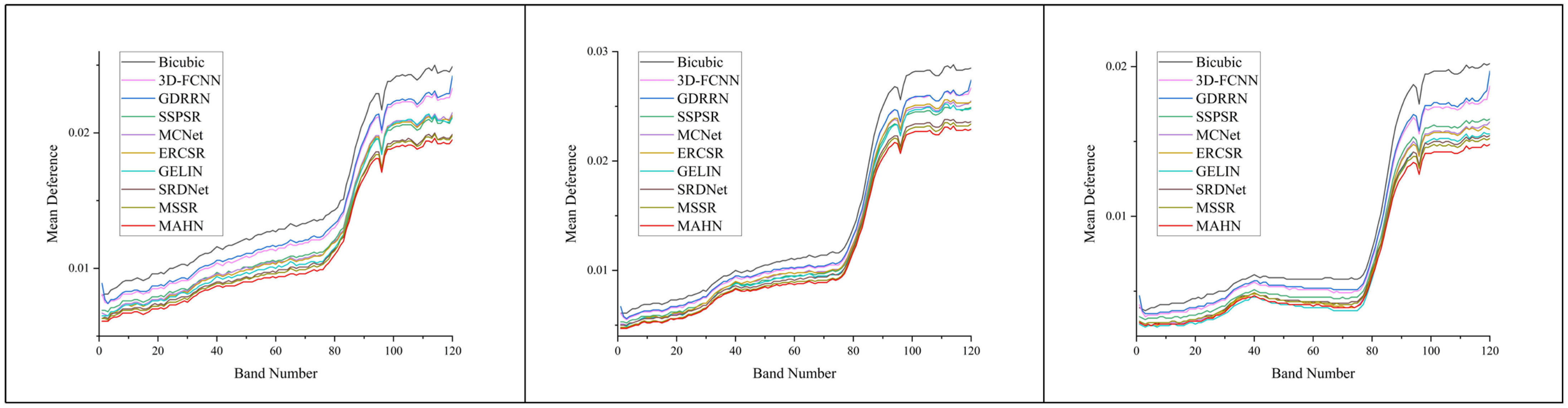
4.2. Results on MDAS

The MDAS multimodal dataset captures images of the city of Augsburg and was published by the Technical University of Munich (TUM). The hyperspectral data contains 368 bands covering a range from 417 to 2484 nm. The images encompass diverse urban scene elements, including vegetation, buildings, and roads. In this experiment, data with a spatial range of $1364\times 1636$ and 120 bands were selected for model training and testing, of which $500\times 500$ was used for testing.

Table 1. Average quantitative comparisons on MDAS dataset by factor 2, 3, and 4.

S	Model	PSNR ↑	SSIM ↑	SAM ↓	ERGAS ↓
2	Bicubic	32.348	0.8664	4.765	15.722
	3D-FCNN [38]	33.137	0.8941	4.473	14.317
	GDRRN [39]	33.034	0.8874	4.572	14.564
	SSPSR [53]	33.790	0.9101	4.166	13.169
	MCNet [24]	33.770	0.9097	4.271	12.959
	ERCSR [25]	33.788	0.9105	4.221	12.926
	GELIN [54]	33.921	0.9143	3.832	12.676
	SRDNet [45]	34.186	0.9186	3.678	12.479
	MSSR [44]	34.322	0.9215	3.325	12.295
	MAHN	34.364	0.9217	3.195	12.218
3	Bicubic	30.308	0.7880	5.968	13.321
	3D-FCNN [38]	30.872	0.8208	5.742	12.415
	GDRRN [39]	30.866	0.8200	5.753	12.400
	SSPSR [53]	-	-	-	-
	MCNet [24]	31.135	0.8313	5.588	11.935
	ERCSR [25]	31.159	0.8328	5.569	11.900
	GELIN [54]	31.234	0.8366	5.151	11.775
	SRDNet [45]	31.430	0.8460	4.911	11.588
	MSSR [44]	31.451	0.8484	4.476	11.522
	MAHN	31.492	0.8513	4.291	11.498
4	Bicubic	29.007	0.7120	7.190	11.501
	3D-FCNN [38]	29.389	0.7452	6.918	10.933
	GDRRN [39]	29.277	0.7221	6.986	11.101
	SSPSR [53]	29.722	0.7663	6.307	10.511
	MCNet [24]	29.604	0.7556	6.832	10.623
	ERCSR [25]	29.602	0.7574	6.887	10.619
	GELIN [54]	29.643	0.7610	6.410	10.541
	SRDNet [45]	29.791	0.7719	6.107	10.457
	MSSR [44]	29.808	0.7745	5.600	10.383
	MAHN	29.820	0.7756	5.445	10.381

shows the performance of various methods on the MDAS dataset. Both SSPSR and GELIN are methods that process spectral bands in groups, effectively reducing the difficulty of spectral feature extraction by decomposing complex spectral signals into multiple sub-signals. By mixing 2D and 3D modules, MCNet and ERCSR effectively reduce the model redundancy and balance the extraction of spatial and spectral information. SRDNet and MSSR introduce 3D convolution and combine multi-domain information for feature supplement. According to the experimental results, our method obtains the optimal numerical results under the three scaling factors. Specifically, in the $2\times$ SR, compared to the sub-optimal results, the four metrics were optimized by 0.042 dB, 0.0002, 0.13, and 0.077, respectively. The SAM of the image reconstructed by our method has a more obvious lead. The SAM under the three magnifications was optimized by 0.13, 0.185, and 0.155, respectively, demonstrating the effectiveness of our method in improving spectral fidelity. The hypergraph constructed based on the high- and low-frequency information of the spectral signals effectively establishes the spectral similarity relationships across different regions. The proposed SHCAM integrates frequency features of the spectral signals across the global range, with the cross-attention mechanism further capturing and enhancing the long-range dependencies between the signals. In order to solve the problem of high coupling of semantic information in low spatial resolution HSI, the hypergraph constructed based on spectral mixture analysis further decouples the complex information in the scene. The experimental results show that the above strategies for spectral information have a very positive effect on improving spectral fidelity.

Figure 3 shows the visualized results and corresponding error heat maps, which are calculated by an absolute error in $4\times$ SR. Figure 4 shows the mean spectral difference curves in $2\times$ SR. It can be observed that the reconstructed edges and textures of our method are clearer, while other methods usually have more obvious blurring and deformation. In the heat map, both numerical values and visual effects, MAHN has a more obvious advantage. In addition, the spectra reconstructed by our method exhibit less distortion, with the advantage being particularly evident in the 100–120th spectral bands.

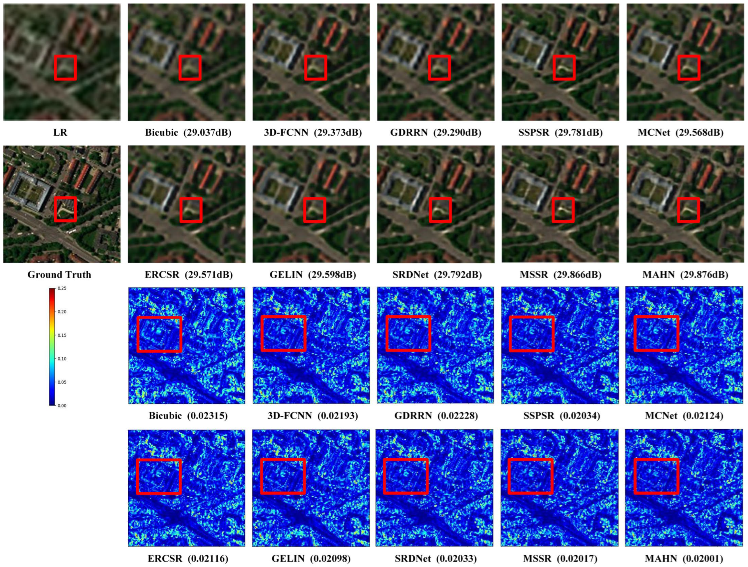
4.3. Results on Pavia Centre

The dataset is an HSI of the central urban area of Pavia, captured by the ROSIS sensor. The image contains 102 bands, with a spectral range of 430–860 nm. The elements in this image mainly consist of houses and roads, representing a typical urban scene. The size of the image is $1096\times 715$, except for the $300\times 200$ area used for testing, the other areas are used for model training.

Table 2. Average quantitative comparisons on Pavia Centre dataset by factors 2, 3, and 4.

S	Model	PSNR ↑	SSIM ↑	SAM ↓	ERGAS ↓
2	Bicubic	32.539	0.9085	4.615	7.820
	3D-FCNN [38]	34.251	0.9370	4.075	6.536
	GDRRN [39]	33.755	0.9240	4.258	6.944
	SSPSR [53]	35.314	0.9475	3.983	5.884
	MCNet [24]	35.587	0.9506	3.749	5.656
	ERCSR [25]	35.612	0.9509	3.726	5.635
	GELIN [54]	35.647	0.9513	3.668	5.614
	SRDNet [45]	35.842	0.9522	3.695	5.573
	MSSR [44]	36.236	0.9552	3.629	5.373
	MAHN	36.313	0.9561	3.541	5.320
3	Bicubic	29.223	0.8062	5.692	7.385
	3D-FCNN [38]	30.410	0.8554	5.223	6.518
	GDRRN [39]	30.121	0.8365	5.463	6.853
	SSPSR [53]	-	-	-	-
	MCNet [24]	31.165	0.8753	5.064	5.999
	ERCSR [25]	31.168	0.8754	5.057	5.986
	GELIN [54]	31.160	0.8753	4.917	6.002
	SRDNet [45]	31.347	0.8793	4.907	5.917
	MSSR [44]	31.547	0.8836	4.768	5.792
	MAHN	31.718	0.8878	4.671	5.685
4	Bicubic	27.284	0.7053	6.313	6.791
	3D-FCNN [38]	28.080	0.7580	6.082	6.242
	GDRRN [39]	27.955	0.7410	6.153	6.212
	SSPSR [53]	28.845	0.7968	5.681	5.739
	MCNet [24]	28.649	0.7867	6.018	5.864
	ERCSR [25]	28.644	0.7869	6.073	5.860
	GELIN [54]	28.630	0.7848	5.814	5.878
	SRDNet [45]	28.786	0.7913	5.918	5.817
	MSSR [44]	28.724	0.7881	5.678	5.843
	MAHN	28.866	0.7964	5.555	5.763

shows the performance of various methods on the Pavia Centre dataset. With scaling factors of 2 and 3, our method achieved the best results on all metrics. In $2\times$ SR, the performance of MCNet, ERCSR, and GELIN shows a significant improvement over earlier methods such as 3D-FCNN and GDRRN. As more novel methods, SRDNet and MSSR further improved the performance. The proposed MAHN achieved higher PSNR and SSIM, and lower SAM and ERGAS. In $3\times$ SR, the advantage of MAHN became more pronounced. Specifically, compared to the sub-optimal results, the proposed method optimized the four metrics by 0.171 dB, 0.0042, 0.097, and 0.107, respectively. In $4\times$ SR, the proposed method achieved two optimal and two sub-optimal metrics. SSPSR, GELIN, and SRDNet all employ a progressive upsampling strategy, which enables them to perform well when facing the challenge of larger scaling factors. Our method constructs different hypergraphs based on high/low-frequency information and high-level semantic spaces, and realizes more accurate reconstruction through the comprehensive characterization of pixel correlation in the global scope. Additionally, the multiple corresponding hypergraph learning modules effectively improved the ability of the model to extract and integrate features. In the red box marked area of Figure 5, the proposed MAHN can better recover small details and alleviate spatial distortion. The error heat maps also demonstrate the significant advantage of our method. The spectral difference curves in Figure 6 reflect that the spectra reconstructed by MAHN have better fidelity.

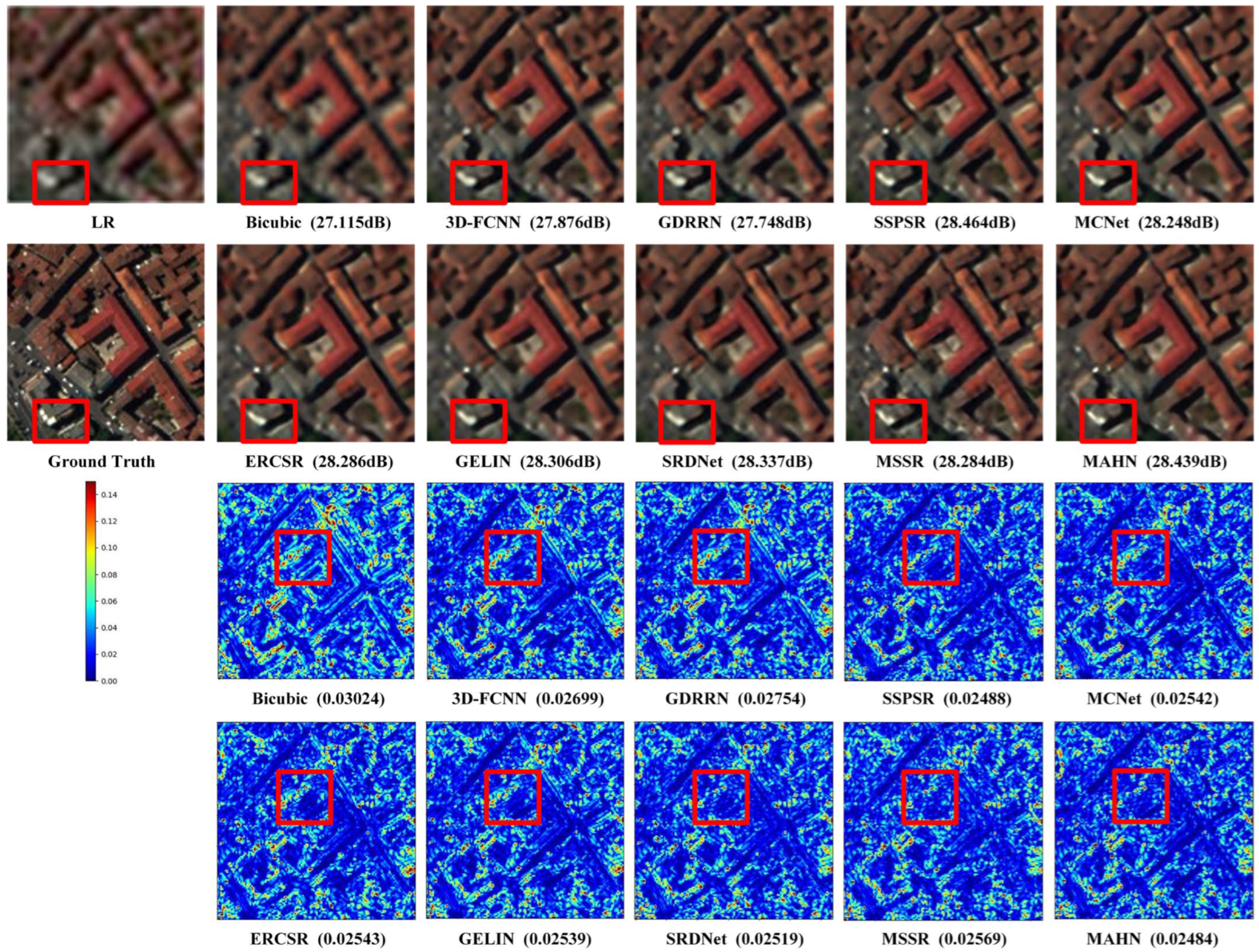
4.4. Results on Houston

The GRSS-DFC-2013-Houston dataset was collected by the National Center for Airborne Laser Mapping at the University of Houston in June 2012 and was distributed for the 2013 IEEE Geoscience and Remote Sensing Society Data Fusion Contest [62]. The HSI contains 144 bands with an imaging spectral range of 380–1050 nm. The size of the complete image is $349\times 1905$, except for the $349\times 400$ area used for testing, the rest of the area is used for model training.

Table 3. Average quantitative comparisons on Houston dataset by factor 2, 3 and 4.

S	Model	PSNR ↑	SSIM ↑	SAM ↓	ERGAS ↓
2	Bicubic	35.854	0.9149	3.680	7.826
	3D-FCNN [38]	36.594	0.9303	3.391	7.235
	GDRRN [39]	36.532	0.9296	3.427	7.300
	SSPSR [53]	37.311	0.9396	3.140	6.647
	MCNet [24]	37.720	0.9437	2.980	6.284
	ERCSR [25]	37.724	0.9436	2.966	6.280
	GELIN [54]	37.764	0.9444	2.913	6.253
	SRDNet [45]	37.896	0.9464	2.720	6.180
	MSSR [44]	38.087	0.9490	2.572	6.058
	MAHN	38.119	0.9491	2.548	6.030
3	Bicubic	33.388	0.8561	4.873	6.624
	3D-FCNN [38]	34.120	0.8785	4.448	6.118
	GDRRN [39]	33.961	0.8762	4.523	6.235
	SSPSR [53]	-	-	-	-
	MCNet [24]	34.718	0.8903	4.165	5.668
	ERCSR [25]	34.766	0.8913	4.137	5.633
	GELIN [54]	34.785	0.8920	4.067	5.631
	SRDNet [45]	34.932	0.8963	3.789	5.546
	MSSR [44]	34.938	0.8971	3.699	5.544
	MAHN	35.004	0.8985	3.605	5.512
4	Bicubic	31.931	0.8026	6.169	5.907
	3D-FCNN [38]	32.587	0.8283	5.618	5.485
	GDRRN [39]	32.489	0.8267	5.677	5.552
	SSPSR [53]	33.124	0.8460	4.967	5.150
	MCNet [24]	32.977	0.8395	5.374	5.218
	ERCSR [25]	32.996	0.8399	5.367	5.206
	GELIN [54]	33.040	0.8413	5.246	5.186
	SRDNet [45]	33.165	0.8471	4.935	5.119
	MSSR [44]	33.145	0.8468	4.808	5.133
	MAHN	33.162	0.8473	4.735	5.132

presents the performance of various methods on the Houston dataset. In $2\times$ and $3\times$ SR, MAHN achieves the best results across all metrics, with PSNR of 38.119 dB (+0.032 dB) and 35.004 dB (+0.066 dB), respectively. In $4\times$ SR, SRDNet achieves the best PSNR and ERGAS, which may be attributed to the progressive upsampling structure used in the hybrid network, allowing it to perform well even with larger upscaling factors. MAHN still demonstrates strong competitiveness, achieving the best SSIM and SAM. This indicates that the hypergraph learning based on high- and low-frequency features can effectively capture both the main structure and subtle changes in the image. In MAHN, hypergraph branches are used to capture global features, while the residual branch is focused on extracting local features. Feature extraction at multiple scales ensures that the network learns both the neighborhood details and long-range dependencies of the information nodes. Overall, our method performs excellently across all three datasets, proving its superiority and robustness. In Figure 7, in the red box marked area of the false-color image, our method reconstructs more realistic road details. Our results also show significantly lower energy in the heat map. Additionally, the spectral difference curves in Figure 8 further demonstrate the advantage of our method, particularly in the 20–70th spectral bands.

5. Discussion

In this section, we will discuss the parameters and computational complexity of the model, the effectiveness of the proposed module, and the potential for SR tasks in real-world scenarios.

5.1. Parameters and Computational Cost

Table 4. Comparison of parameter quantity, computation amount, and inference time.

Model	PSNR ↑	Parameters (M)	GFLOPs	Inference Time/Per Frame (s)
SSPSR [53]	33.790	11.1	90.29	0.0348
MCNet [24]	33.770	1.9	236.61	0.0162
ERCSR [25]	33.788	1.3	178.84	0.0088
GELIN [54]	33.921	26.7	563.65	0.1305
SRDNet [45]	34.186	1.7	92.29	0.0162
MSSR [44]	34.322	24.5	49.64	0.0116
MAHN	34.364	4.3	14.72	0.0136

provides the number of parameters, computational cost and inference time of each model in $2\times$ SR task of the MDAS dataset. In terms of the number of parameters, MCNet, ERCSR and SRDNet have fewer parameters and are all models constructed around 3D convolution. Compared with traditional 2D convolution, 3D convolution can not only extract spectral features more efficiently, but also generate fewer network parameters. GELIN and MSSR have relatively complex network structures and also generate more network parameters. Although our method has multiple branches and involves multiple types of features, it does not take up too many parameters, which benefits from the more direct learning process in hypergraph learning. In terms of computational cost, our method demonstrates a significant advantage. The three methods based on 3D convolutions exhibit higher computational cost, which is related to the inherent calculation mode of 3D convolutions. Generally speaking, the process of hypergraph learning only involves matrix multiplication, which significantly reduces the computational cost. When considering performance, parameter efficiency, computational overhead, and inference speed together, our method demonstrates strong practical applicability and deployment potential.

5.2. Ablation Study

To validate the effectiveness of the proposed method, we conducted ablation experiments focusing on multiple information extraction branches and the SBAM. These experiments were carried out on the $2\times$ SR task for the MDAS dataset. Various combinations of the modules are used to verify the effect of each module on the performance of the model.

Table 5. Average quantitative comparisons among some variants of the proposed method on MDAS by factor 2.

SBAM	SHCAM	SHSAM	SH3M	PSNR ↑	SSIM ↑	SAM ↓	ERGAS ↓
				34.107	0.9155	3.523	12.668
√	√			34.156	0.9170	3.472	12.549
√		√		34.144	0.9167	3.480	12.600
√			√	34.174	0.9181	3.453	12.531
√	√	√		34.235	0.9195	3.422	12.476
√	√		√	34.216	0.9189	3.441	12.503
√		√	√	34.271	0.9204	3.371	12.421
	√	√	√	34.296	0.9211	3.356	12.356
√	√	√	√	34.364	0.9217	3.195	12.218

presents the quantitative results of the ablation experiments. When only one of the three hypergraph learning branches was retained, SH3M appeared to provide the greatest performance improvement, with the four metrics optimized by 0.067 dB, 0.0026, 0.07, and 0.137, respectively. When two branches were retained, the combination of SHSAM and SH3M yielded even better results. The addition of SBAM also led to a noticeable improvement. Overall, the learning modules for multiple feature spaces have a positive impact on the results. By extracting and representing multi-domain information, these modules provide richer guidance for image reconstruction. The attention mechanism based on sensitive bands connects multiple branches and strengthens the fusion of cross-domain information.

5.3. SR for Real HSIs

All the experiments above used synthetic datasets for training and testing, and the proposed MAHN demonstrated excellent performance. In this section, we will validate the performance of MAHN in real-world scenarios. Specifically, the experiment is focused on the $4\times$ SR task, where the model is trained on the Pavia Centre dataset and tested on the Pavia University dataset. The Pavia University dataset was captured by the ROSIS sensor as well, with 103 spectral bands spanning a range of 430–860 nm. To match the input dimensions of the model, we retained only the first 102 spectral bands. The natural image quality evaluator (NIQE) was chosen as the objective evaluation metric. Figure 9 presents the visualization results of each model, with NIQE scores labeled below the images. Both the visual effects and quantitative metrics indicate the effectiveness and superiority of our method. The experiment on real-world scenarios proves the application potential of the proposed MAHN.

6. Limitations

In terms of the computational cost of the proposed model, compared to other methods, our approach has achieved relatively superior performance. However, there remains a possibility for further optimization regarding parameter count. Since the algorithm proposed in this paper is targeted at remote sensing hyperspectral images, continued exploration of the potential for reducing model size holds significant importance for enabling future onboard real-time processing.

In addition, although MAHN has demonstrated superior performance in various scenarios, methods based on hypergraph learning still warrant further discussion. Most hypergraph learning strategies rely on pre-defined mathematical models or specific domain knowledge. However, real-world data often contains complex, non-linear relationships that may not be adequately captured within static frameworks. In the future, the construction of hypergraphs should be more flexible, adjusting dynamically to the characteristics of the data and the requirements of the task. Introducing constraints that better align with actual physical systems could further enhance the performance of hypergraph learning in specific applications.

7. Conclusions

In this paper, we propose a hybrid network for HSI SR, named MAHN, which alleviates the challenge of highly coupled complex information in HSIs by more comprehensive extraction and representation of frequency and semantic features, thus achieving precise reconstruction of fine textures and spectral characteristics. Specifically, we designed a multi-branch feature extraction network. On the one hand, based on spectral and spatial frequency hypergraphs, SHCAM and SHSAM are designed to capture the multi-dimensional main structures and subtle changes within the image. On the other hand, an unmixing algorithm is employed to extract the abundance of components in mixed pixels, and the SH3M is proposed to facilitate the propagation and reorganization of high-level semantic information. Additionally, to achieve better cross-domain feature fusion, we introduce the SBAM for the interaction between different feature spaces. By extracting the spatial and spectral frequency features of the image as well as pixel-level semantics, the high-order global relationships are modeled, thereby achieving a comprehensive representation of the internal information of the image. Comparative experiments on multiple datasets demonstrate that, compared to other state-of-the-art methods, the proposed MAHN achieves superior performance and lower computational costs. For real-world SR tasks, our method also reconstructs more realistic texture details, showcasing its potential for practical applications.

References

1. Wu, G.Y.; Al-qaness, M.A.A.; Al-Alimi, D.; Dahou, A.; Abd Elaziz, M.; Ewees, A.A. Hyperspectral image classification using graph convolutional network: A comprehensive review. Expert Syst. Appl. 2024, 257, 125106. [Google Scholar] [CrossRef]
2. Wang, L.Q.; Zhu, T.C.; Kumar, N.; Li, Z.W.; Wu, C.L.; Zhang, P.Y. Attentive-adaptive network for hyperspectral images classification with noisy labels. IEEE Trans. Geosci. Remote Sens. 2023, 61, 3254159. [Google Scholar] [CrossRef]
3. Feng, H.; Wang, Y.C.; Chen, C.; Xu, D.D.; Zhao, Z.K.; Zhao, T.Q. Hyperspectral image classification framework based on multichannel graph convolutional networks and class-guided attention mechanism. IEEE Trans. Geosci. Remote Sens. 2024, 62, 3388429. [Google Scholar] [CrossRef]
4. Tu, B.; Yang, X.C.; He, W.; Li, J.; Plaza, A. Hyperspectral anomaly detection using reconstruction fusion of quaternion frequency domain analysis. IEEE Trans. Neural Netw. Learn. Syst. 2024, 35, 8358–8372. [Google Scholar] [CrossRef] [PubMed]
5. Shen, X.F.; Liu, H.J.; Nie, J.; Zhou, X.C. Matrix factorization with framelet and saliency priors for hyperspectral anomaly detection. IEEE Trans. Geosci. Remote Sens. 2023, 61, 3248599. [Google Scholar] [CrossRef]
6. Liu, S.H.; Song, M.P.; Xue, B.; Chang, C.; Zhang, M.J. Hyperspectral real-time local anomaly detection based on finite markov via line-by-line processing. IEEE Trans. Geosci. Remote Sens. 2024, 62, 3345941. [Google Scholar] [CrossRef]
7. Gomez, R.B.; Jazaeri, A.; Kafatos, M. Wavelet-based hyperspectral and multispectral image fusion. In Proceedings of the Conference on Geo-Spatial Image and Data Exploitation II, Orlando, FL, USA, 16 April 2001; pp. 36–42. [Google Scholar]
8. Zhang, Y.F.; De Backer, S.; Scheunders, P. Noise-resistant wavelet-based bayesian fusion of multispectral and hyperspectral images. IEEE Trans. Geosci. Remote Sens. 2009, 47, 3834–3843. [Google Scholar] [CrossRef]
9. Hardie, R.C.; Eismann, M.T.; Wilson, G.L. Map estimation for hyperspectral image resolution enhancement using an auxiliary sensor. IEEE Trans. Image Process. 2004, 13, 1174–1184. [Google Scholar] [CrossRef]
10. Eismann, M.T.; Hardie, R.C. Application of the stochastic mixing model to hyperspectral resolution, enhancement. IEEE Trans. Geosci. Remote Sens. 2004, 42, 1924–1933. [Google Scholar] [CrossRef]
11. Yokoya, N.; Yairi, T.; Iwasaki, A. Coupled nonnegative matrix factorization unmixing for hyperspectral and multispectral data fusion. IEEE Trans. Geosci. Remote Sens. 2012, 50, 528–537. [Google Scholar] [CrossRef]
12. Bendoumi, M.A.; He, M.Y.; Mei, S.H. Hyperspectral image resolution enhancement using high-resolution multispectral image based on spectral unmixing. IEEE Trans. Geosci. Remote Sens. 2014, 52, 6574–6583. [Google Scholar] [CrossRef]
13. Li, X.; Xu, F.; Liu, F.; Lyu, X.; Tong, Y.; Xu, Z.; Zhou, J. A synergistical attention model for semantic segmentation of remote sensing images. IEEE Trans. Geosci. Remote Sens. 2023, 61, 3243954. [Google Scholar] [CrossRef]
14. Sun, Z.Z.; Leng, X.G.; Zhang, X.H.; Zhou, Z.; Xiong, B.L.; Ji, K.F.; Kuang, G.Y. Arbitrary-direction sar ship detection method for multiscale imbalance. IEEE Trans. Geosci. Remote Sens. 2025, 63, 3559701. [Google Scholar]
15. Zhang, X.H.; Zhang, S.Q.; Sun, Z.Z.; Liu, C.F.; Sun, Y.L.; Ji, K.F.; Kuang, G.Y. Cross-sensor sar image target detection based on dynamic feature discrimination and center-aware calibration. IEEE Trans. Geosci. Remote Sens. 2025, 63, 3559618. [Google Scholar] [CrossRef]
16. Li, X.; Xu, F.; Liu, F.; Tong, Y.; Lyu, X.; Zhou, J. Semantic segmentation of remote sensing images by interactive representation refinement and geometric prior-guided inference. IEEE Trans. Geosci. Remote Sens. 2023, 62, 3339291. [Google Scholar] [CrossRef]
17. Li, X.; Xu, F.; Tao, F.F.; Tong, Y.; Gao, H.M.; Liu, F.; Chen, Z.Q.; Lyu, X. A cross-domain coupling network for semantic segmentation of remote sensing images. IEEE Geosci. Remote Sens. Lett. 2024, 21, 3477609. [Google Scholar] [CrossRef]
18. Xie, Q.; Zhou, M.H.; Zhao, Q.; Meng, D.Y.; Zuo, W.M.; Xu, Z.B.; Soc, I.C. Multispectral and hyperspectral image fusion by ms/hs fusion net. In Proceedings of the 32nd IEEE/CVF Conference on Computer Vision and Pattern Recognition (CVPR), Long Beach, CA, USA, 16–20 June 2019; IEEE Computer Soc: Long Beach, CA, USA, 2019; pp. 1585–1594. [Google Scholar]
19. Dian, R.W.; Li, S.T.; Kang, X.D. Regularizing hyperspectral and multispectral image fusion by cnn denoiser. IEEE Trans. Neural Netw. Learn. Syst. 2021, 32, 1124–1135. [Google Scholar] [CrossRef]
20. Zheng, Y.X.; Li, J.J.; Li, Y.S.; Guo, J.; Wu, X.Y.; Chanussot, J. Hyperspectral pansharpening using deep prior and dual attention residual network. IEEE Trans. Geosci. Remote Sens. 2020, 58, 8059–8076. [Google Scholar] [CrossRef]
21. Dong, W.Q.; Yang, Y.F.; Qu, J.H.; Xie, W.Y.; Li, Y.S. Fusion of hyperspectral and panchromatic images using generative adversarial network and image segmentation. IEEE Trans. Geosci. Remote Sens. 2022, 60, 3078711. [Google Scholar] [CrossRef]
22. Wang, X.Y.; Ma, J.Y.; Jiang, J.J. Hyperspectral image super-resolution via recurrent feedback embedding and spatialspectral consistency regularization. IEEE Trans. Geosci. Remote Sens. 2022, 60, 3064450. [Google Scholar]
23. Tang, Y.; Li, J.; Yue, L.W.; Liu, X.X.; Li, Y.J.; Xiao, Y.; Yuan, Q.Q. A cnn-transformer embedded unfolding network for hyperspectral image super-resolution. IEEE Trans. Geosci. Remote Sens. 2024, 62, 3431924. [Google Scholar] [CrossRef]
24. Li, Q.; Wang, Q.; Li, X.L. Mixed 2d/3d convolutional network for hyperspectral image super-resolution. Remote Sens. 2020, 12, 1660. [Google Scholar] [CrossRef]
25. Li, Q.; Wang, Q.; Li, X.L. Exploring the relationship between 2d/3d convolution for hyperspectral image super-resolution. IEEE Trans. Geosci. Remote Sens. 2021, 59, 8693–8703. [Google Scholar] [CrossRef]
26. Li, X.; Xu, F.; Yu, A.Z.; Lyu, X.; Gao, H.M.; Zhou, J. A frequency decoupling network for semantic segmentation of remote sensing images. IEEE Trans. Geosci. Remote Sens. 2025, 63, 3531879. [Google Scholar] [CrossRef]
27. Li, X.; Xu, F.; Li, L.Y.; Xu, N.; Liu, F.; Yuan, C.; Chen, Z.Q.; Lyu, X. Aaformer: Attention-attended transformer for semantic segmentation of remote sensing images. IEEE Geosci. Remote Sens. Lett. 2024, 21, 3397851. [Google Scholar] [CrossRef]
28. Feng, Y.F.; You, H.X.; Zhang, Z.Z.; Ji, R.R.; Gao, Y. Hypergraph Neural Networks. In Proceedings of the 33rd AAAI Conference on Artificial Intelligence/31st Innovative Applications of Artificial Intelligence Conference/9th AAAI Symposium on Educational Advances in Artificial Intelligence, Honolulu, HI, USA, 27 Jan–1 February 2019; pp. 3558–3565. [Google Scholar]
29. Ronneberger, O.; Fischer, P.; Brox, T. U-net: Convolutional networks for biomedical image segmentation. In Proceedings of the 18th International Conference on Medical Image Computing and Computer-Assisted Intervention (MICCAI), Munich, Germany, 5–9 October 2015; pp. 234–241. [Google Scholar]
30. Qu, J.H.; Shi, Y.Z.; Xie, W.Y.; Li, Y.S.; Wu, X.Y.; Du, Q. Mssl: Hyperspectral and panchromatic images fusion via multiresolution spatialspectral feature learning networks. IEEE Trans. Geosci. Remote Sens. 2022, 60, 318962. [Google Scholar] [CrossRef]
31. Zhuo, Y.W.; Zhang, T.J.; Hu, J.F.; Dou, H.X.; Huang, T.Z.; Deng, L.J. A deep-shallow fusion network with multidetail extractor and spectral attention for hyperspectral pansharpening. IEEE J. Sel. Top. Appl. Earth Observ. Remote Sens. 2022, 15, 7539–7555. [Google Scholar] [CrossRef]
32. He, L.; Xie, J.H.; Li, J.; Plaza, A.; Chanussot, J.; Zhu, J.W. Variable subpixel convolution based arbitrary-resolution hyperspectral pansharpening. IEEE Trans. Geosci. Remote Sens. 2022, 60, 3189624. [Google Scholar] [CrossRef]
33. Zhang, L.; Nie, J.T.; Wei, W.; Zhang, Y.N.; Liao, S.C.; Shao, L. Unsupervised adaptation learning for hyperspectral imagery super-resolution. In Proceedings of the IEEE/CVF Conference on Computer Vision and Pattern Recognition (CVPR), Seattle, WA, USA, 14–19 June 2020; pp. 3070–3079. [Google Scholar]
34. Guo, Z.L.; Xin, J.W.; Wang, N.N.; Li, J.; Gao, X.B. External-internal attention for hyperspectral image super-resolution. IEEE Trans. Geosci. Remote Sens. 2022, 60, 3207230. [Google Scholar] [CrossRef]
35. Hong, D.F.; Yao, J.; Li, C.Y.; Meng, D.Y.; Yokoya, N.; Chanussot, J. Decoupled-and-coupled networks: Self-supervised hyperspectral image super-resolution with subpixel fusion. IEEE Trans. Geosci. Remote Sens. 2023, 61, 3324497. [Google Scholar] [CrossRef]
36. Zheng, K.; Gao, L.R.; Liao, W.Z.; Hong, D.F.; Zhang, B.; Cui, X.M.; Chanussot, J. Coupled convolutional neural network with adaptive response function learning for unsupervised hyperspectral super resolution. IEEE Trans. Geosci. Remote Sens. 2021, 59, 2487–2502. [Google Scholar] [CrossRef]
37. Sun, W.W.; Ren, K.; Meng, X.C.; Xiao, C.C.; Yang, G.; Peng, J.T. A band divide-and-conquer multispectral and hyperspectral image fusion method. IEEE Trans. Geosci. Remote Sens. 2022, 60, 3046321. [Google Scholar] [CrossRef]
38. Mei, S.H.; Yuan, X.; Ji, J.Y.; Zhang, Y.F.; Wan, S.; Du, Q. Hyperspectral image spatial super-resolution via 3d full convolutional neural network. Remote Sens. 2017, 9, 1139. [Google Scholar] [CrossRef]
39. Li, Y.; Zhang, L.; Ding, C.; Wei, W.; Zhang, Y.N. Single hyperspectral image super-resolution with grouped deep recursive residual network. In Proceedings of the 4th IEEE International Conference on Multimedia Big Data (BigMM), Xi’an, China, 13–16 September 2018; pp. 1–4. [Google Scholar]
40. Dong, C.; Loy, C.C.G.; He, K.M.; Tang, X.O. Learning a deep convolutional network for image super-resolution. In Proceedings of the 13th European Conference on Computer Vision (ECCV), Zurich, Switzerland, 6–12 September 2014; Springer International Publishing Ag: Zurich, Switzerland, 2014; pp. 184–199. [Google Scholar]
41. Tai, Y.; Yang, J.; Liu, X.M. Image super-resolution via deep recursive residual network. In Proceedings of the 30th IEEE/CVF Conference on Computer Vision and Pattern Recognition (CVPR), Honolulu, HI, USA, 21–26 July 2017; pp. 2790–2798. [Google Scholar]
42. Li, J.J.; Cui, R.X.; Li, B.; Song, R.; Li, Y.S.; Dai, Y.C.; Du, Q. Hyperspectral image super-resolution by band attention through adversarial learning. IEEE Trans. Geosci. Remote Sens. 2020, 58, 4304–4318. [Google Scholar] [CrossRef]
43. Wang, Q.; Li, Q.; Li, X.L. Hyperspectral image superresolution using spectrum and feature context. IEEE Trans. Ind. Electron. 2021, 68, 11276–11285. [Google Scholar] [CrossRef]
44. Chen, C.; Wang, Y.C.; Zhang, Y.X.; Zhao, Z.K.; Feng, H. Remote sensing hyperspectral image super-resolution via multidomain spatial information and multiscale spectral information fusion. IEEE Trans. Geosci. Remote Sens. 2024, 62, 3388531. [Google Scholar] [CrossRef]
45. Liu, T.T.; Liu, Y.; Zhang, C.C.; Yuan, L.Y.; Sui, X.B.; Chen, Q. Hyperspectral image super-resolution via dual-domain network based on hybrid convolution. IEEE Trans. Geosci. Remote Sens. 2024, 62, 3370107. [Google Scholar] [CrossRef]
46. Liu, Y.T.; Hu, J.W.; Kang, X.D.; Luo, J.; Fan, S.S. Interactformer: Interactive transformer and cnn for hyperspectral image super-resolution. IEEE Trans. Geosci. Remote Sens. 2022, 60, 3183468. [Google Scholar] [CrossRef]
47. Wu, Y.M.; Cao, R.H.; Hu, Y.K.; Wang, J.; Li, K.L. Combining global receptive field and spatial spectral information for single-image hyperspectral super-resolution. Neurocomputing 2023, 542, 126277. [Google Scholar] [CrossRef]
48. Hu, Q.; Wang, X.Y.; Jiang, J.J.; Zhang, X.P.; Ma, J.Y. Exploring the spectral prior for hyperspectral image super-resolution. IEEE Trans. Image Process. 2024, 33, 5260–5272. [Google Scholar] [CrossRef]
49. Yuan, Y.; Zheng, X.T.; Lu, X.Q. Hyperspectral image superresolution by transfer learning. IEEE J. Sel. Top. Appl. Earth Observ. Remote Sens. 2017, 10, 1963–1974. [Google Scholar] [CrossRef]
50. Cheng, Y.S.; Wang, X.Y.; Ma, Y.; Mei, X.G.; Wu, M.H.; Ma, J.Y. General hyperspectral image super-resolution via meta-transfer learning. IEEE Trans. Neural Netw. Learn. Syst. 2024, 36, 6134–6147. [Google Scholar] [CrossRef] [PubMed]
51. Rombach, R.; Blattmann, A.; Lorenz, D.; Esser, P.; Ommer, B. High-resolution image synthesis with latent diffusion models. In Proceedings of the IEEE/CVF Conference on Computer Vision and Pattern Recognition (CVPR), New Orleans, LA, USA, 18–24 June 2022; pp. 10674–10685. [Google Scholar]
52. Pang, L.; Rui, X.; Cui, L.; Wang, H.; Meng, D.; Cao, X. HIR-Diff: Unsupervised hyperspectral image restoration via improved diffusion models. In Proceedings of the IEEE/CVF Conference on Computer Vision and Pattern Recognition (CVPR), Seattle, WA, USA, 17–18 June 2024; pp. 3005–3014. [Google Scholar] [CrossRef]
53. Jiang, J.J.; Sun, H.; Liu, X.M.; Ma, J.Y. Learning spatial-spectral prior for super-resolution of hyperspectral imagery. IEEE Trans. Comput. Imaging 2020, 6, 1082–1096. [Google Scholar] [CrossRef]
54. Wang, X.Y.; Hu, Q.; Jiang, J.J.; Ma, J.Y. A group-based embedding learning and integration network for hyperspectral image super-resolution. IEEE Trans. Geosci. Remote Sens. 2022, 60, 3217406. [Google Scholar] [CrossRef]
55. Wang, H.; Wang, C.; Yuan, Y. Asymmetric dual-direction quasi-recursive network for single hyperspectral image super-resolution. IEEE Trans. Circuits Syst. Video Technol. 2023, 33, 6331–6346. [Google Scholar] [CrossRef]
56. Zhao, M.H.; Ning, J.W.; Hu, J.; Li, T.T. Attention-driven dual feature guidance for hyperspectral super-resolution. IEEE Trans. Geosci. Remote Sens. 2023, 61, 3318013. [Google Scholar] [CrossRef]
57. Mei, Z.Y.; Bi, X.; Li, D.G.; Xia, W.; Yang, F.; Wu, H. Dhhnn: A dynamic hypergraph hyperbolic neural network based on variational autoencoder for multimodal data integration and node classification. Inf. Fusion 2025, 119, 103016. [Google Scholar] [CrossRef]
58. Ding, J.W.; Tan, Z.Y.; Lu, G.M.; Wei, J.S. Hypergraph denoising neural network for session-based recommendation. Appl. Intell. 2025, 55, 391. [Google Scholar] [CrossRef]
59. Wang, Z.; Bovik, A.C.; Sheikh, H.R.; Simoncelli, E.P. Image quality assessment: From error visibility to structural similarity. IEEE Trans. Image Process. 2004, 13, 600–612. [Google Scholar] [CrossRef]
60. Kruse, F.A.; Lefkoff, A.B.; Boardman, J.W.; Heidebrecht, K.B.; Shapiro, A.T.; Barloon, P.J.; Goetz, A.F.H. The spectral image processing system (sips)—Interactive visualization and analysis of imaging spectrometer data. Remote Sens. Environ. 1993, 44, 145–163. [Google Scholar] [CrossRef]
61. Wald, L. Quality of high resolution synthesised images: Is there a simple criterion? In Proceedings of the Third Conference Fusion of Earth Data: Merging Point Measurements, Raster Maps and Remotely Sensed Images, Cannes, France, 6 February 2000; pp. 99–103. [Google Scholar]
62. Debes, C.; Merentitis, A.; Heremans, R.; Hahn, J.; Frangiadakis, N.; van Kasteren, T.; Liao, W.Z.; Bellens, R.; Pizurica, A.; Gautama, S.; et al. Hyperspectral and lidar data fusion: Outcome of the 2013 grss data fusion contest. IEEE J. Sel. Top. Appl. Earth Observ. Remote Sens. 2014, 7, 2405–2418. [Google Scholar] [CrossRef]
Figure 1. The structure of the proposed MAHN. The input LR image is fed into four feature extraction branches, namely Spectral-Net, Spatial-Net, Semantic-Net, and Res-Net. Furthermore, through the sensitive band attention module, the cross-fusion and guidance of features in multiple branches are achieved.
Remotesensing 17 01947 g001
Figure 2. The illustration of the proposed SHCAM (a), SHSAM (b), and SH3M (c). The feature extraction modules for spectral (a), spatial (b) and semantic (c) information, respectively, utilize the multi-head cross-attention mechanism, the multi-head self-attention mechanism, and 3D CNN.
Remotesensing 17 01947 g002
Figure 3. Reconstructed images and corresponding error heat maps from MDAS dataset in 4× SR.
Remotesensing 17 01947 g003
Figure 4. Mean spectral difference curves from MDAS dataset in 2× SR.
Remotesensing 17 01947 g004
Figure 5. Reconstructed images and corresponding error heat maps from Pavia Centre dataset in 4× SR.
Remotesensing 17 01947 g005
Figure 6. Mean spectral difference curves from Pavia Centre dataset in 2× SR.
Remotesensing 17 01947 g006
Figure 7. Reconstructed images and corresponding error heat maps from Houston dataset in 4× SR.
Remotesensing 17 01947 g007
Figure 8. Mean spectral difference curves from Houston dataset in 2× SR.
Remotesensing 17 01947 g008
Figure 9. Reconstructed images of a real scene from Pavia University dataset for the 4× SR.
Remotesensing 17 01947 g009