An Autofocus Method for Long Synthetic Time and Large Swath Synthetic Aperture Radar Imaging Under Multiple Non-Ideal Factors

Abstract

Synthetic aperture radar (SAR) is an all-weather and all-day imaging technique for Earth observation. Achieving efficient observation, high resolution, and wide swath coverage have remained critical development goals in SAR technology, which inherently require extended synthetic aperture time. However, various non-ideal factors, including atmospheric disturbances, orbital perturbations, and antenna vibrations. degrade imaging performance, causing defocusing and ghost targets. Furthermore, the long synthetic time and large imaging swath further enlarge the temporal and spatial variability of these factors and seriously degrade the imaging effect. These inherent challenges make autofocusing indispensable for SAR imaging with a long synthetic time and large swath. In this paper, a novel autofocus method specifically designed to address these non-ideal factors is proposed for SAR imaging with a long synthetic time and large swath. The innovation of the method mainly consists of two parts. The first is the autofocus for multiple non-ideal factors, which is accomplished by an improved phase gradient autofocus (PGA) equipped with amplitude error estimation and discrete windowing. PGA with amplitude error estimation can solve the problem of defocus, and discrete windowing can focus the energy of paired echoes. The second is an error fusion and interpolation method for a long synthetic time and large swath. This method fuses errors among sub-apertures in the long synthetic time and can fulfill autofocus for blocks where strong scatterers are not sufficient in the large swath. The proposed method can effectively achieve SAR focusing with a long synthetic time and large swath, considering spatial and temporal variant non-ideal factors. Point target simulations and distributed target simulations based on real scenarios are conducted to validate the proposed method.

1. Introduction

Synthetic aperture radar (SAR) is an active microwave imaging technology capable of all-weather, all-day Earth observation, demonstrating broad application prospects in disaster monitoring, resource exploration, and building condition assessment [1,2,3]. With continuous advancements in SAR technology, SAR imaging is progressively evolving toward longer synthetic times and larger swaths to meet the demands of high-efficiency and high-precision mapping. Geosynchronous SAR (GEO SAR) [4,5] is a typical long-synthetic-time large-swath SAR, and current research has yielded significant work in areas such as system analysis and design [6,7,8,9], two-dimensional (2-D) imaging processing [10,11,12,13,14,15,16], three-dimensional imaging processing, and deformation extraction [17,18,19], etc. Some preliminary equivalent experiments have been performed to validate the principle and feasibility of these SAR systems [20,21]. Furthermore, leveraging its extremely high orbital altitude, moon-based SAR (MB SAR) [22,23] possesses inherent advantages in wide-swath imaging, giving rise to moon-based SAR Earth observation technology. Current research efforts focus on system design and signal processing of MB SAR [24,25,26], elevating SAR mapping coverage to new heights and further advancing long-synthetic-time large-swath SAR technology development.

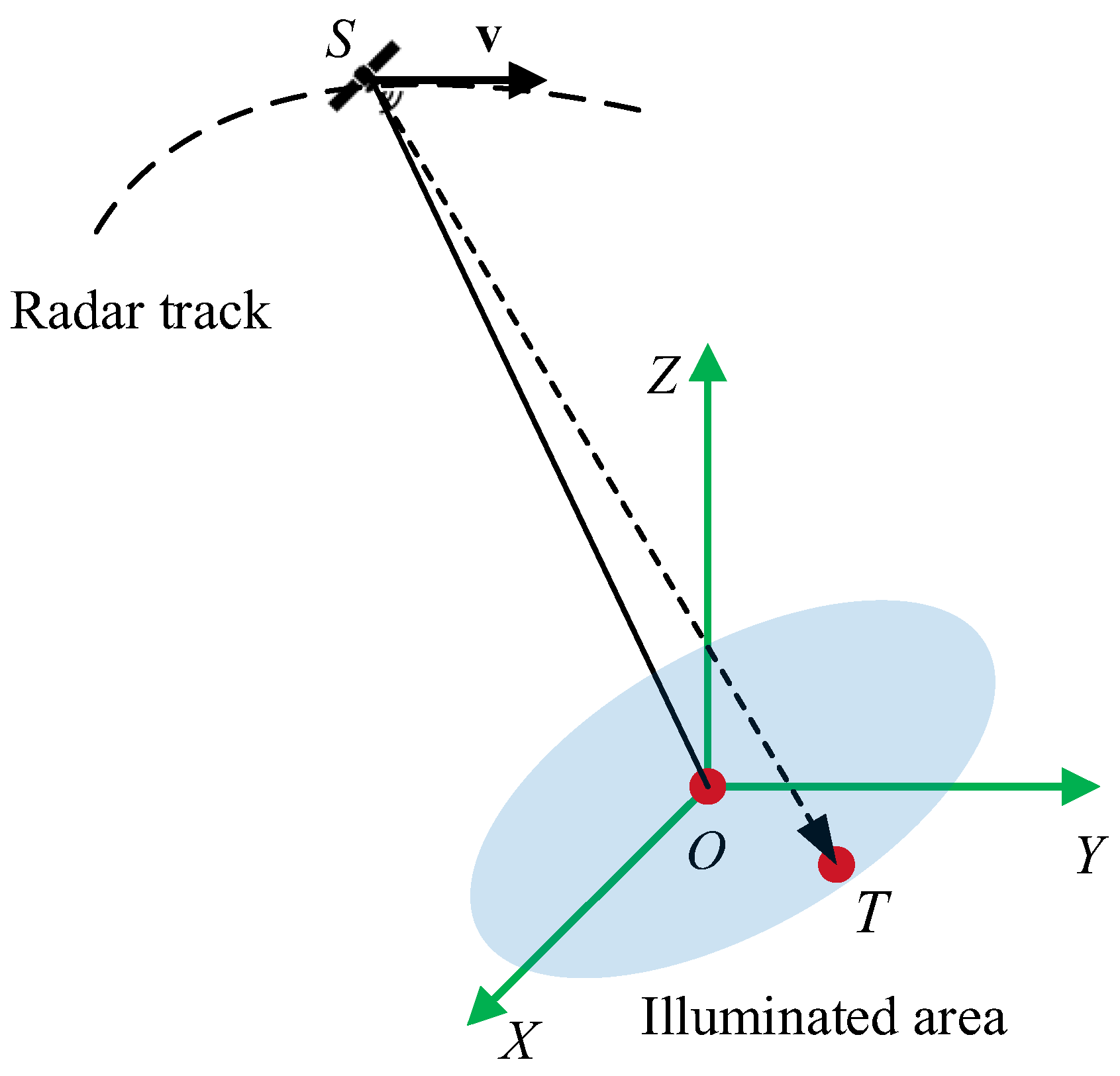
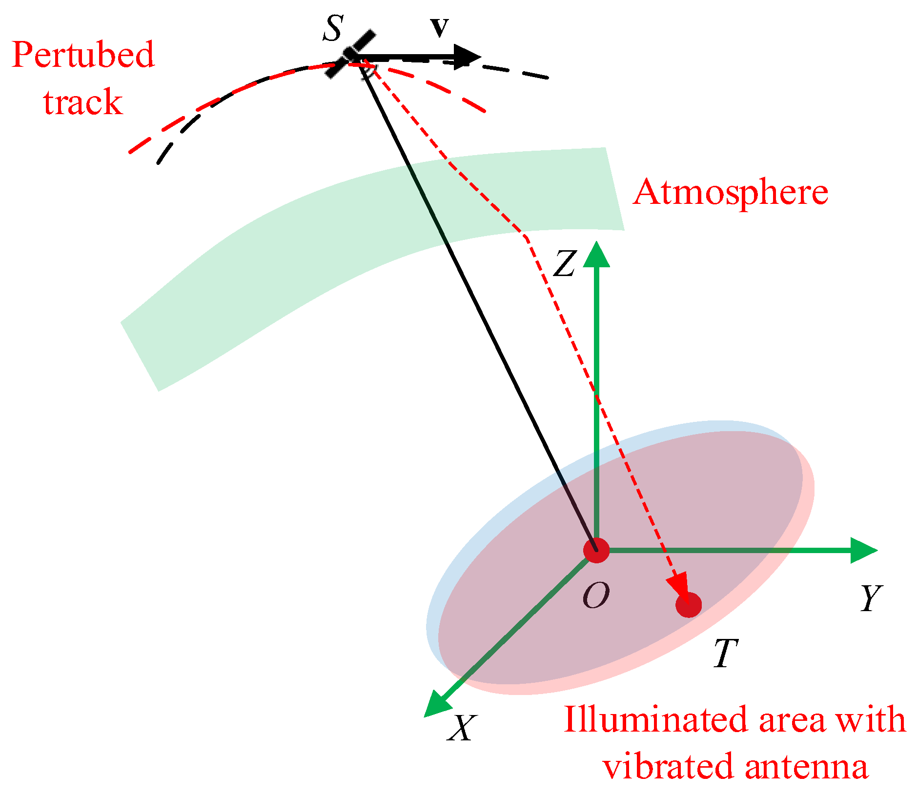
However, due to the influence of extremely long synthetic aperture times and large swaths, many non-ideal factors, including atmospheric impact, orbital perturbation, and antenna vibration, will result in seriously undesired impacts on SAR images. Therefore, these factors must be taken into account in SAR imaging processing. At the same time, due to the curved trajectory and the large imaging width, the impact of these non-ideal factors also has serious 2-D spatial variation characteristics. Therefore, analysis of and compensation for these non-ideal factors are hotspots of current SAR research [27].

At present, many studies have been carried out on non-ideal factors. The sources and effects of these non-ideal factors can be summarized as follows:

• Atmospheric impact [28,29,30,31,32,33,34]: The electromagnetic waves of SAR will travel through the atmosphere twice, and the atmosphere will affect the SAR signal. The atmospheric impact mainly includes three aspects: background ionosphere, ionospheric scintillation, and the tropospheric impact. The background ionosphere mainly brings polynomial phase errors, and it will degrade focusing performance by spreading the mainlobe and introducing asymmetric sidelobes. Ionospheric scintillation will bring random phase and amplitude errors, which will mainly affect focusing performance by degrading the integrated sidelobe ratio (ISLR).
• Orbital perturbation [35,36,37,38]: Theoretically, the orbit information of GEO SAR or MB SAR can be obtained from the ephemeris. However, non-ideal factors such as J2 perturbation, third body perturbation, and radiation pressure perturbation will make the real orbit deviate from the theoretical orbit, which leads to undesired orbital perturbations. Generally, orbital perturbation can be partially compensated for based on high precision orbit determination technology. However, the precision of orbit determination is usually worse than several centimeters, which is comparable to the wavelength, and the residue error after compensation still cannot be neglected. Thus, it is necessary to deal with the residual orbital perturbation error after compensation based on orbital determination technology, which is also the focus of the term “orbital perturbation error” in this paper.
• Antenna vibration [39,40]: Due to the large physical size of GEO SAR and MB antennae, which are usually dozens of meters, SAR with a long synthetic time and large swath is faced with severe antenna vibration, which consists of translational vibration and rotational vibration. Antenna translational vibration will result in the periodic phase error, and antenna rotational vibration will cause periodic amplitude error. Further information related to the impact of antenna vibration on SAR can be found in [40].

To deal with these non-ideal factors of SAR with a long synthetic time and large swath, several methods have been proposed, and these methods can be divided into two types. One is the SAR autofocusing method based on persistent scatterers (PSs) [41,42,43]. These methods regard the PSs as point targets and extract the errors from these point targets directly. The other type is the SAR autofocusing method based on optimal image quality [44,45,46,47]. Image quality evaluation indices, such as entropy, contrast, sharpness, or correlation with the real image, are used in this type of method. This method establishes the relationship between image quality and non-ideal factors, and the non-ideal factors can be estimated adaptively and iteratively.

However, the methods mentioned above have unneglectable shortcomings. The methods based on PSs in [41,42,43] consider only one type of the non-ideal factors, and the effectiveness of the methods still remain to be validated for actual SAR working conditions with multiple non-ideal factors. As for the methods based on optimal image quality in [44,45,46,47], iteration is usually required for optimization. In this case, the calculation burden becomes an unneglectable problem. In addition, the selection of a proper image quality index is also a problem for error estimation.

To resolve the aforementioned problems and obtain well-focused SAR images, an autofocusing method for SAR with a long synthetic time and large swath is proposed. The main contributions are twofold.

• The method provides a PGA-based solution to SAR imaging with multi-source non-ideal factors. Specifically, an improved phase gradient autofocus equipped with discrete windowing and amplitude error estimation is proposed to deal with multiple types of error.
• An error fusion and interpolation method is proposed to deal with the problem of error estimation with a long synthetic time and large swath. This method fuses errors among sub-apertures in the long synthetic time and can fulfill autofocus for blocks where strong scatterers are not sufficient in the large swath. The error in these blocks is interpolated with the errors in adjacent blocks which have sufficient PSs.

The steps of the proposed method are delivered as follows. This method firstly takes 2-D blocking for the scenery to deal with the range and azimuth spatial variability of the non-ideal factor impacts. Subsequently, synthetic aperture division is applied to reduce the temporal variability of the non-ideal factor impacts. Afterwards, the spectral analysis (SPECAN) algorithm is used for imaging, which facilitates error compensations in the azimuth time domain. The errors are estimated with an improved PGA algorithm, which uses the phase gradient of strong points to estimate the phase error and uses the envelope to estimate the amplitude error. In addition, the discrete windowing technique is applied to extract strong points in the condition of the paired echoes. The proposed method can be applied to SAR with a long synthetic time and large swath. Considering that MB SAR, which involves long-synthetic-aperture-time and large-swath imaging, still has a significant gap from practical application, this paper conducts modeling, derivation, and simulation with reference to the observation geometry of GEO SAR.

The rest of this paper is organized as follows. In Section 2, the SAR echo signal model considering non-ideal factors is discussed. In Section 3, the autofocusing method is derived and proposed in detail. Section 4 validates the proposed method via computer simulations based on the target array and the distributed target. Finally, the conclusions are delivered in Section 5.

2. SAR Echo Signal Model Considering Multiple Non-Ideal Factors

SAR imaging with a long synthetic time and large swath is faced with multiple non-ideal factors. In this section, SAR signaling is modelled under two conditions: the ideal condition and the condition with the impact of non-ideal factors. Different types of amplitude and phase errors caused by the non-ideal factors are also analyzed in this section.

2.1. Ideal SAR Signal Model

The geometry of SAR with a long synthetic time and large swath is shown in Figure 1. Here, the origin of the coordinate system is the center of the illuminated area. The Y-axis is parallel with the velocity of the radar in the center of synthetic aperture, the Z-axis is perpendicular to the local earth surface, and the X-axis is determined by right-hand rule. In this coordinate system, the coordinates of radar $\overrightarrow{S}(t_a)$ can be modeled as a function that slowly changes with time, where $t_a$ is the slow time, namely the azimuth time. Correspondingly, for a target with position vector $\overrightarrow{T}$ in the scene, its slant range history can be expressed by Taylor series as [15]

$$R\left(t_a;R_p,t_p\right)=‖\overrightarrow{ST}‖\approx R_p+k_1\left(t_a-t_p\right)+k_2{\left(t_a-t_p\right)}^2+k_3{\left(t_a-t_p\right)}^3+k_4{\left(t_a-t_p\right)}^4$$

(1)

where $t_p$ is the beam center crossing time for the target and $R_p$ is the corresponding instantaneous slant range between the target and radar when $t_a=t_p$. Moreover, it should be noted that, for other targets with different positions in the scene, the coefficients $k_i, i=1,2,3,4$ have significant spatial variance and are related to $t_p$ and $R_p$.

Correspondingly, taking no account of non-ideal factors and considering that the transmitted signal is linearly frequency modulated with chirp rate $k_r$, the SAR signal can be written as

$$s_{\mathrm{ideal}}\left(t_r,t_a\right)=u_r\left[{\displaystyle \frac{t_r-\frac{2\cdot R\left(t_a\right)}{c}}{T_p}}\right]u_a\left[t_a-t_p\right]\exp \left[j\pi k_r{\left(t_r-{\displaystyle \frac{2\cdot R\left(t_a\right)}{c}}\right)}^2\right]\exp \left[-j{\displaystyle \frac{4\pi R\left(t_a\right)}{\lambda }}\right]$$

(2)

where $u_r\left[\cdot \right]$ and $u_a\left[\cdot \right]$ are range and azimuth windows, respectively. $t_r$ is the fast time, namely the range time, $T_p$ is the pulse duration, $\lambda$ is the wavelength, and $c$ is the speed of light.

2.2. Actual SAR Signal Model Considering Non-Ideal Factors

As is shown in Figure 2, non-ideal factors such as atmosphere, orbital perturbation, and antenna vibration are unavoidable for an actual SAR system with a long synthetic time and large swath. These non-ideal factors will introduce significant errors in SAR signaling, including polynomial phase errors, random amplitude and phase errors, and periodic amplitude and phase errors. In this subsection, a brief introduction to these errors will be delivered, and the analytical expression of the SAR signal affected by these non-ideal factors will be given.

2.2.1. Polynomial Phase Error

The polynomial phase errors of SAR are mainly caused by background ionosphere delay and orbital perturbation. These two non-ideal factors will be discussed in the following parts in turn.

The SAR signal will travel through the atmosphere twice, and the atmospheric impact, which generally includes ionospheric and tropospheric impact, should be taken into consideration, due to the extremely high orbital height. This article focuses on SAR working at a low carrier frequency; thus, the tropospheric impact can be omitted, and only the ionospheric impact on the SAR signal is taken into account, which consists of the background ionosphere delay and the ionospheric scintillation. Here, only the background ionosphere delay will lead to polynomial phase error, and the ionospheric scintillation will be discussed in the section on random errors.

When the SAR signal travels through the ionosphere, an additional delay related to the total electron content (TEC) of background ionosphere will be added to the slant range [33]:

$$\Delta {\varphi }_{\mathrm{BI}}=-{\displaystyle \frac{4\pi \cdot \Delta R}{\lambda }}=-{\displaystyle \frac{2\pi \cdot 80.6\cdot TEC}{c\cdot f}}$$

(3)

where $TEC$ is the total electron content, and its units are total electron content units (TECU, 1 TECU = 10¹⁶ electrons per meter squared). $f$ is the frequency of the signal, and the subscript BI is the abbreviation for background ionosphere. Furthermore, it should be noted that, due to the limited range bandwidth of the SAR signal and the medium typical values of TEC, dispersion related to the background ionosphere is usually dismissed [28], so (3) can be rewritten as

$$\Delta {\varphi }_{\mathrm{BI}}=-{\displaystyle \frac{2\pi \cdot 80.6\cdot TEC}{c\cdot f_0}}$$

(4)

where $f_0$ is the carrier frequency.

For SAR with an extremely long aperture time, TEC is not constant during the entire beam illuminating process, and it should be modeled as a function of slow time. In addition, due to the wide imaging swath of SAR, the spatial variance of TEC cannot be ignored, and it should be modeled as a function of the target position. In summary, TEC can be written as [33]

$$TEC\left(t_a;\overrightarrow{T}\right)=TE{C}_0\left(\overrightarrow{T}\right)+k_1^{TEC}\left(\overrightarrow{T}\right)t_a+k_2^{TEC}\left(\overrightarrow{T}\right)t_a^2+k_3^{TEC}\left(\overrightarrow{T}\right)t_a^3$$

(5)

where $TE{C}_0$ is the time-invariant part of TEC and $k_1^{TEC}$~$k_3^{TEC}$ are the time variant coefficients of TEC.

Further information about ionosphere modelling can be found in [48]. In [48], the background ionosphere model, as well as the ionospheric scintillation model mentioned in the following subsection, is validated with a real data equivalent experiment using GPS signaling.

As for the orbital perturbation, the non-spherical gravitation force, luni-solar perturbations, and solar radiation pressure will introduce unneglectable orbital perturbation errors into the SAR platform. In general, orbital perturbations can be described with fluctuating orbital elements, and theses fluctuating orbital elements will bring Doppler parameter errors. Moreover, the corresponding Doppler phase error caused by the orbital perturbation can be written as

$$\Delta {\varphi }_{\mathrm{OP}}=2\pi \left(\Delta f_{d1}\cdot t_a+{\displaystyle \frac{\Delta f_{d2}}{2}}\cdot t_a^2+{\displaystyle \frac{\Delta f_{d3}}{6}}\cdot t_a^3+{\displaystyle \frac{\Delta f_{d4}}{24}}\cdot t_a^4\right)$$

(6)

where the subscript OP denotes orbital perturbation, and the SAR signal considering the polynomial phase error caused by the background ionosphere and the orbital perturbation can be modeled as

$$s_{\mathrm{Poly}}\left(t_r,t_a\right)=s_{\mathrm{ideal}}\left(t_r,t_a\right)\exp \left(j\Delta {\varphi }_{\mathrm{OP}}\right)\exp \left(j\Delta {\varphi }_{\mathrm{BI}}\right)$$

(7)

2.2.2. Random Amplitude and Phase Error

The random phase and amplitude errors of SAR with a long synthetic time and large swath are caused by ionospheric scintillation [49]. When the signal travels through the ionosphere, the ionospheric scintillation will cause both amplitude and phase fluctuations in the signal, and these fluctuations can be modeled as slow time varying random amplitude and phase as

$$E_{\mathrm{IS}}={\delta }_{\mathrm{IS}}\left(t_a\right)\exp \left[j{\varphi }_{\mathrm{IS}}\left(t_a\right)\right]$$

(8)

where ${\delta }_{\mathrm{IS}}$ and ${\varphi }_{\mathrm{IS}}$ are fluctuating amplitude and phase, respectively, and the subscript IS denotes ionospheric scintillation. Moreover, it should be noted that both ${\delta }_{\mathrm{IS}}$ and ${\varphi }_{\mathrm{IS}}$ are spatially variant.

The SAR signal considering random phase and amplitude errors can be written as

$$s_{\mathrm{Rand}}\left(t_r,t_a\right)=s_{\mathrm{ideal}}\left(t_r,t_a\right){\delta }_{\mathrm{IS}}\left(t_a\right)\exp \left[j{\varphi }_{\mathrm{IS}}\left(t_a\right)\right]$$

(9)

2.2.3. Periodic Amplitude and Phase Error

The periodic phase and amplitude errors of SAR with a long synthetic time and large swath is caused by antenna vibration.

For SAR working in the L-band, its antenna size might be several meters or even longer [39], so that its vibration cannot be dismissed during imaging processing with a long synthetic aperture time. Antenna vibration of SAR mainly includes two parts, namely rotational vibration and translational vibration, and they will cause gain error and slant range error, respectively.

For the sake of simplicity, and without loss of generality, a single-frequency periodic translational vibration is first taken into account, and the slant range error is

$$\Delta R_{\mathrm{AT}}={\displaystyle \frac{\lambda }{4\pi }}{A}_T\sin \left(2\pi f_T{t}_a+{\phi }_T\right)$$

(10)

where $A_T$, $f_T$, and ${\phi }_T$ are the amplitude, frequency, and initial phase of translational vibration, respectively. Correspondingly, a Doppler phase error will be introduced to the signal as

$$s_{\mathrm{AT}}\left(t_r,t_a\right)=s_{\mathrm{ideal}}\left(t_r,t_a\right)\exp \left[-j{A}_T\sin \left(2\pi f_T{t}_a+{\phi }_T\right)\right]$$

(11)

As for the rotational vibration, it mainly influences the direction of the beam, and thus brings a gain error. Generally, the antenna gain affected by the rotational vibration can be modeled as a periodic amplitude error $g_{\mathrm{AR}}\left(t_a\right)$ of slow time. Further explanation for the periodic amplitude error is given in [40].

Taking both translational and rotational vibration into consideration, the actual SAR signal can be expressed as

$$s_{\mathrm{Period}}\left(t_r,t_a\right)=g_{\mathrm{AR}}\left(t_a\right)s_{\mathrm{ideal}}\left(t_r,t_a\right)\exp \left[-j{A}_T\sin \left(2\pi f_T{t}_a+{\phi }_T\right)\right]$$

(12)

2.2.4. Summary

Based on the aforementioned discussions about non-ideal factors, the actual SAR echo signal can be written as

$$s_{\mathrm{actual}}\left(t_r,t_a\right)=s_{\mathrm{ideal}}\left(t_r,t_a\right)g_E\left(t_a\right)\exp \left[j{\phi }_E\left(t_a\right)\right]$$

(13)

where $g_E\left(t_a\right)$ and ${\phi }_E\left(t_a\right)$ denote the overall amplitude and phase errors, respectively. As mentioned before, $g_E\left(t_a\right)$ consists of a slowly time-variant part and a random time-variant part, which are related to the antenna rotational vibration and the ionospheric scintillation, and it can be written as

$$g_E\left(t_a\right)=g_{\mathrm{AR}}\left(t_a\right){\delta }_{\mathrm{IS}}\left(t_a\right)$$

(14)

As for ${\phi }_E\left(t_a\right)$, it is the sum of three parts: a polynomial term related to errors caused by background ionosphere and orbital perturbation, a periodic term introduced by antenna translational vibration, and a random error due to ionospheric scintillation. In summary, ${\phi }_E\left(t_a\right)$ can be written as

$${\phi }_{\mathrm{E}}\left(t_a\right)={\displaystyle \sum _{i=1}^4{K}_i{t}_a^i+}{A}_{\mathrm{T}}\cos \left(2\pi f_{\mathrm{T}}{t}_a+{\phi }_{\mathrm{T}}\right)+{\varphi }_{\mathrm{IS}}\left(t_a\right)$$

(15)

where $K_i,i=1,2,3,4$ denote the overall polynomial coefficients of polynomial phase errors such as background ionosphere error and orbital perturbation error.

3. An Improved Phased Gradient Autofocus Method for SAR with a Long Synthetic Time and Large Swath

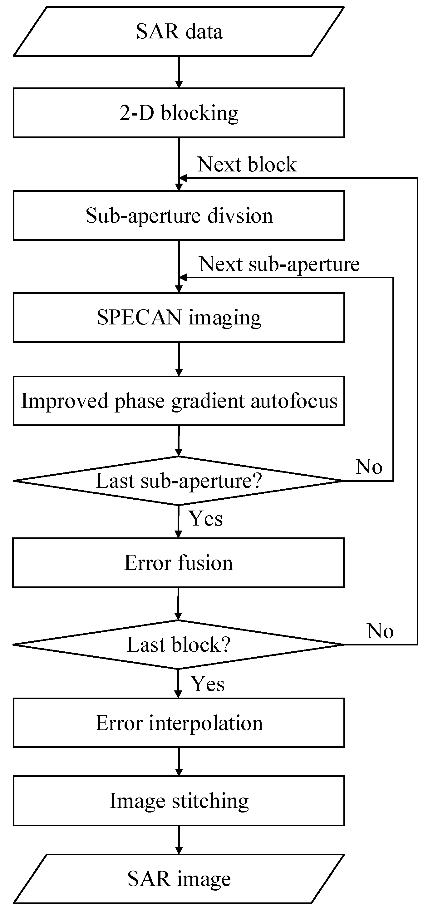
To deal with the undesired impacts on SAR imaging with a long synthetic time and large swath caused by the aforementioned multiple non-ideal factors, an autofocus method based on SPECAN imaging and an improved PGA algorithm are proposed in this section. The method involves 2-D blocking, synthetic aperture division, and discrete windowing, and the overall flowchart of the method is shown in Figure 3. The detailed process flow of the proposed method will be introduced as follows.

3.1. 2-D Blocking and Synthetic Aperture Division

As discussed before, the impacts caused by non-ideal factors show severe 2-D spatial variability, which will significantly increase the difficulty of autofocus processing. To address this problem, the characteristics of 2-D spatial variance are analyzed, and 2-D blocking is adopted. 2-D blocking is a valid approach to deal with the problem of spatial variance. After a scene with an extremely large width is divided into several small blocks, the spatial variance problems will no longer exist within each block. The block size can be restricted by the overall high order phase error, and discussion on the block size can be found in [44]. In order to facilitate the image stitching process afterwards, the blocks are set with overlap. The size of the overlapped area can be set as several tens of samples.

GEO SAR satellite works at a 36,000-kilometer-high orbit, and MB SAR works with a distance of 380,000 km on average. These will result in an unsatisfactory noise equivalent sigma zero (NESZ). With a full aperture time as long as hundreds of seconds, low SNR and large error will cause totally defocused strong points, which will lead to a failure of phase error estimation in autofocus methods related to a strong point, such as the PGA algorithm.

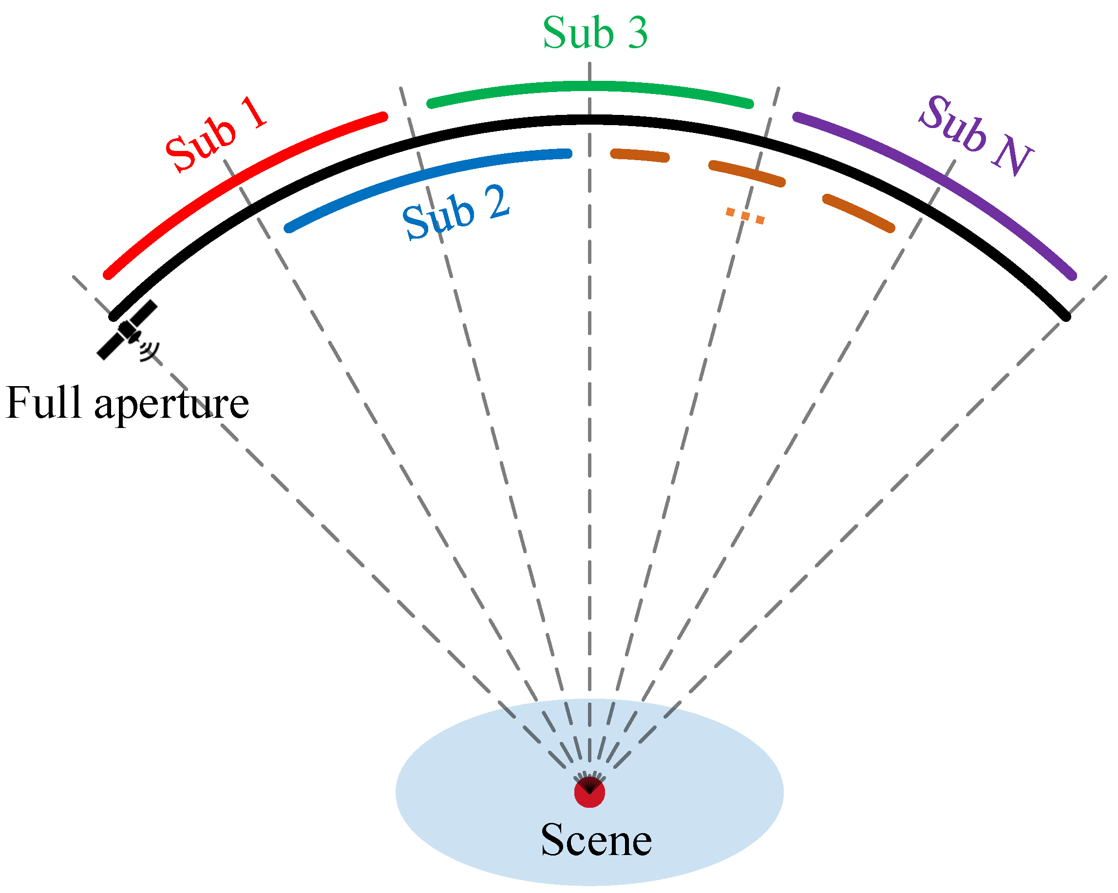
Therefore, the problem of effective raw focusing should be addressed first, and dividing the full synthetic aperture to several short sub-apertures can be an applicable approach to solve the problem. As shown in Figure 4, in each sub-aperture, phase error is limited within an appropriate range so that the defocusing level of the strong point will not be too severe, raw imaging will be accomplished properly via the SPECAN algorithm, and the phase errors can be estimated separately. There are overlaps between each adjacent sub-aperture pair, with which error fusion can be accomplished after error estimation.

The length of each sub-aperture can be preliminarily set according to typical parameters or otherwise observed non-ideal factor parameters, and imaging can be realized with the preliminary sub-aperture time. If imaging processing fails, a shorter length can be chosen until enough almost-well-focused strong points are acquired.

3.2. SPECAN Imaging

For each sub-aperture and in each block, imaging is fulfilled with the SPECAN algorithm. The typical SPECAN algorithm consist of range compression and range cell migration correction in the range frequency domain, deramping in the azimuth time domain, and finally azimuth Fourier transformation. As for SPECAN imaging for SAR with a long synthetic time and large swath, considering the non-ideal factors, range processing and RCMC can be easily performed within each sub-aperture and each block, and the result can be written as

$$s_{\mathrm{RC}}\left(t_r,t_a\right)=\sin \mathrm{c}\left[B_r\left(t_r-{\displaystyle \frac{2R_p}{c}}\right)\right]\exp \left[-j{\displaystyle \frac{4\pi R\left(t_a\right)}{\lambda }}\right]\times g_E\left(t_a\right)\exp \left[j{\phi }_E\left(t_a\right)\right]$$

(16)

where $g_E\left(t_a\right)$ and ${\phi }_E\left(t_a\right)$ denote the overall non-ideal amplitude and phase error, which is discussed in (15) and (16).

For the range compressed signal $s_{\mathrm{RC}}\left(t_r,t_a\right)$, azimuth compression can be realized via a high-order phase multiplication and azimuth Fourier transformation

$$s_{\mathrm{AC}}\left(t_r,f_a\right)={\mathrm{FFT}}_a\left\{s_{\mathrm{RC}}\left(t_r,t_a\right)\times h_{\mathrm{AC}}\left(t_a\right)\right\}$$

(17)

where

$$h_{\mathrm{AC}}\left(t_a\right)=\exp \left[j{\displaystyle \frac{4\pi }{\lambda }}\left(R_p+k_1{t}_a+k_2{t}_a^2+k_3{t}_a^3+k_4{t}_a^4\right)\right]$$

(18)

Combining (17) and (18), with some high-order terms omitted, the azimuth compressed result is

$$\begin{array}{c}{s}_{\mathrm{AC}}\left(t_r,f_a\right)=\sin \mathrm{c}\left[B_r\left(t_r-{\displaystyle \frac{2R_p}{c}}\right)\right]\sin \mathrm{c}\left[T_a\left(f_a+{\displaystyle \frac{4k_2{t}_p}{\lambda }}\right)\right]\\ \ast {\mathrm{FFT}}_a\left\{g_E\left(t_a\right)\right\}\ast {\mathrm{FFT}}_a\left\{\exp \left[j{\phi }_E\left(t_a\right)\right]\right\}\end{array}$$

(19)

where * denotes convolution.

With the stationary phase principle, method of series inversion, and Jacobi–Anger expansion, the non-ideal phase in the azimuth frequency domain can be written as

$$\begin{array}{l}{\mathrm{FFT}}_a\left\{\exp \left[j{\phi }_E\left(t_a\right)\right]\right\}=S_{\mathrm{E}}^{\mathrm{poly}}\left(f_a\right)\ast S_{\mathrm{E}}^{\mathrm{period}}\left(f_a\right)\ast S_{\mathrm{E}}^{\mathrm{rand}}\left(f_a\right)\\ \approx S_{\mathrm{E}}^{\mathrm{poly}}\left(f_a\right)J_0\left(A_{\mathrm{T}}\right)+{\displaystyle \sum _{n\ne 0}{j}^n{J}_n\left(A_{\mathrm{T}}\right)S_{\mathrm{E}}^{\mathrm{poly}}\left(f_a+n{f}_{\mathrm{T}}\right)\exp \left(j{\phi }_{\mathrm{T}}\right)}\end{array}$$

(20)

where $J_n\left(\cdot \right)$ represents the Bessel function of the first kind. This result shows that periodic errors in azimuth imaging manifest as paired echoes, which replicate the image along the azimuth direction with specific weights. The replication interval relates to the vibration frequency, while the weighting factors depend on vibration amplitude and initial phase. In (20), the polynomial phase error can be written as

$$S_{\mathrm{E}}^{\mathrm{poly}}\left(f_a\right)=\exp \left[j\left(K_1^f{f}_a+K_2^f{f}_a^2+K_3^f{f}_a^3+K_4^f{f}_a^4\right)\right]$$

(21)

and the random phase $S_{\mathrm{E}}^{\mathrm{rand}}\left(f_a\right)$ is omitted, for it can hardly be described with an analytical expression, and it can be analyzed via statistical methods. Here the coefficients can be calculated with the method of series inversion:

$$K_n^f={\displaystyle \frac{1}{n{K}_1^n}}{\displaystyle \sum _{s,t,u,\dots }{(-1)}^{s+t+u+\dots }\frac{n(n+1)\cdots (n-1+s+t+u+\dots )}{s!t!u!\cdots }{\left(\frac{K_2}{K_1}\right)}^s{\left(\frac{K_3}{K_1}\right)}^t\cdots }$$

(22)

As for the amplitude error, considering the fact that it will be estimated in the azimuth time domain by extracting the envelope of strong targets, its analytical form is not required. As a result, the final signal model after SPECAN imaging can be achieved as

$$\begin{array}{cc}{s}_{\mathrm{AC}}\left(t_r,f_a\right)=& \sin \mathrm{c}\left[B_r\left(t_r-{\displaystyle \frac{2R_p}{c}}\right)\right]\sin \mathrm{c}\left[T_a\left(f_a+{\displaystyle \frac{4k_2{t}_p}{\lambda }}\right)\right]\\ & \ast {\mathrm{FFT}}_a\left\{g_E\left(t_a\right)\right\}\ast S_{\mathrm{E}}^{\mathrm{poly}}\left(f_a\right)\ast S_{\mathrm{E}}^{\mathrm{period}}\left(f_a\right)\ast S_{\mathrm{E}}^{\mathrm{rand}}\left(f_a\right)\end{array}$$

(23)

According to the SPECAN imaging result, the final image of a point target can be seen as an ideal 2-D sinc function convolved with the spectra of the errors, which will degrade the quality of the image through widening the mainlobe and causing paired echoes.

3.3. Improved Phase Gradient Autofocus

In the following autofocus processing, an improved phased gradient autofocus is applied to estimate and compensate for the errors. The main differences of the proposed improved PGA and traditional PGA involve two aspects: (1) discrete windowing, rather than the rectangular windowing in traditional PGA, is applied to deal with the paired echoes introduced by periodic errors; and (2) an envelope of strong targets is extracted to estimate the amplitude errors. In addition, the phase errors are estimated in the same way of traditional PGA processing.

3.3.1. Discrete Windowing

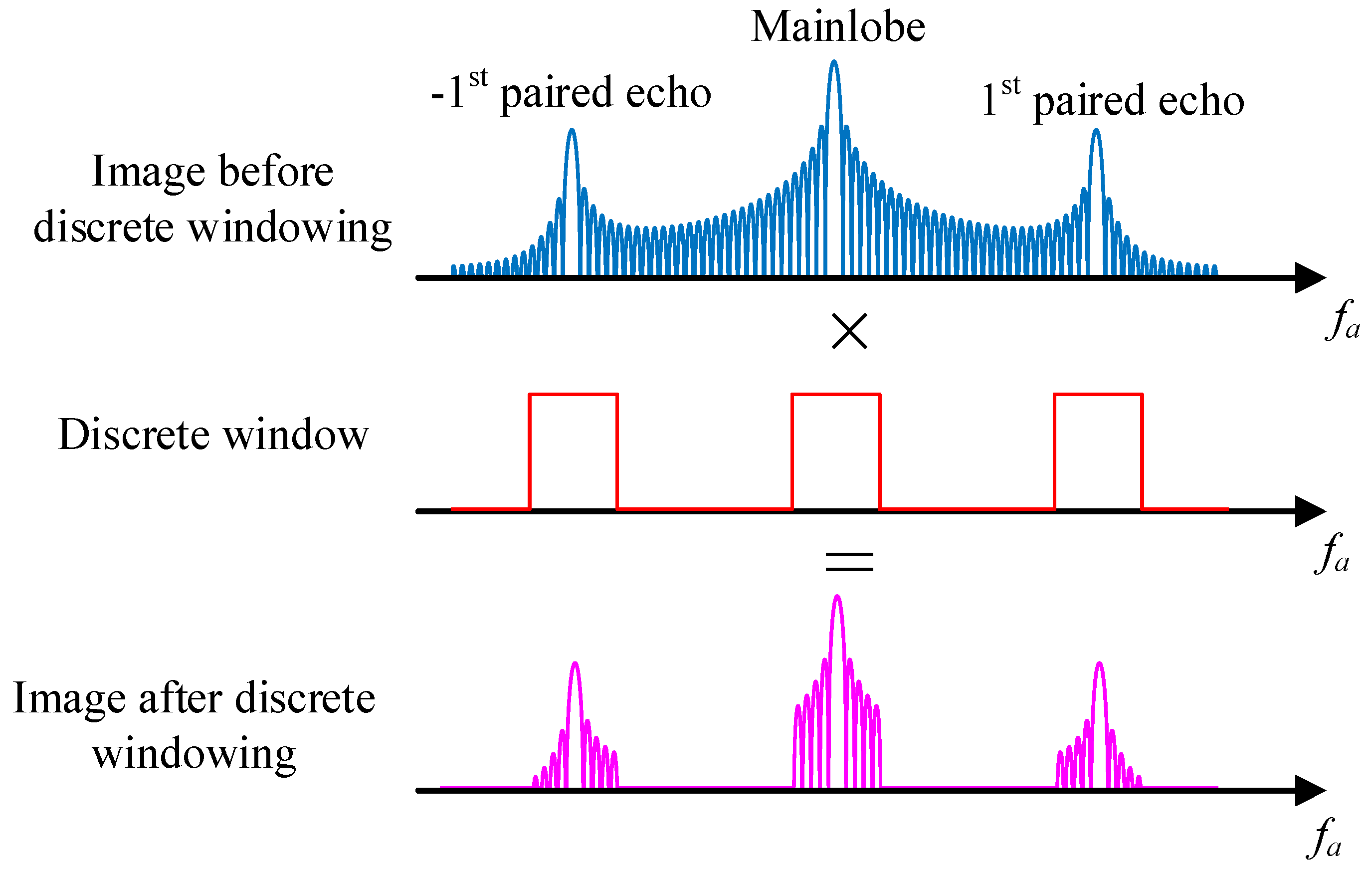
The periodic phase error caused by antenna vibration will bring extra paired echo peaks in the image, thus spreading the energy of the targets. As is shown in (20), the paired echo peaks appear in the position with azimuth displacement of integer multiples of vibration frequency from the actual mainlobe position

$$f_{\mathrm{pe}}^n=-{\displaystyle \frac{4k_2{t}_p}{\lambda }}+n{f}_{\mathrm{T}},n=\pm 1,\pm 2,\dots$$

(24)

where $f_{\mathrm{pe}}^n$ is the position of the nth paired echo in the image. As a result, the power of the strong point is mainly distributed discretely in the neighborhoods around the peaks of the mainlobe and the paired echoes.

The discrete windowing method can be applied to address the problem of paired echoes. As shown in Figure 5, the basic idea of discrete windowing is to multiply the data with a series of discrete windows which have non-zero values only near the mainlobe and the paired echo peaks, and thus include the energy of the target as much as possible.

Considering the SPECAN processing in (23), and taking the widened azimuth point spread function as a whole, the azimuth image is

$$\begin{array}{l}{s}_{\mathrm{AC}}\left(f_a\right)=p_a\left(f_a\right)\ast S_{\mathrm{E}}^{\mathrm{period}}\left(f_a\right)\\ =p_a\left(f_a\right)J_0\left(A_{\mathrm{T}}\right)+{\displaystyle \sum _{n\ne 0}{j}^n{J}_n\left(A_{\mathrm{T}}\right)p_a\left(f_a+n{f}_{\mathrm{T}}\right)\exp \left(j{\phi }_{\mathrm{T}}\right)}\end{array}$$

(25)

where the widened azimuth point spread function is

$$p_a\left(f_a\right)=\sin \mathrm{c}\left[T_a\left(f_a+{\displaystyle \frac{4k_2{t}_p}{\lambda }}\right)\right]\ast {\mathrm{FFT}}_a\left\{g_E\left(t_a\right)\right\}\ast S_{\mathrm{E}}^{\mathrm{poly}}\left(f_a\right)\ast S_{\mathrm{E}}^{\mathrm{rand}}\left(f_a\right)$$

(26)

A series of discrete windows can be defined as

$$W_{\mathrm{D}}\left(f_a\right)={\displaystyle \sum _{n=-N\mathrm{D}}^{N_{\mathrm{D}}}W\left(\frac{f_a+n{f}_{\mathrm{T}}}{L_n}\right)}$$

(27)

where $W\left(\cdot \right)$ is rectangular window function. The total number of discrete windows is $2N_{\mathrm{D}}+1$, and the width of each window $L_n$ is determined by the power distribution of each peak in the same way as traditional continuous windowing. After discrete windowing, the image becomes

$$\begin{array}{l}{P}_{\mathrm{f}}\left(f_a\right)=s_{\mathrm{AC}}\left(f_a\right)W_{\mathrm{D}}\left(f_a\right)\\ =p_{aw}\left(f_a\right)J_0\left(A_{\mathrm{T}}\right)+{\displaystyle \sum _{\begin{array}{c}n\ne 0\\ -N\mathrm{D}\le n\le N\mathrm{D}\end{array}}{j}^n{J}_n\left(A_{\mathrm{T}}\right)p_{aw}\left(f_a+n{f}_{\mathrm{T}}\right)\exp \left(j{\phi }_{\mathrm{T}}\right)}\end{array}$$

(28)

where $p_{aw}\left(f_a+n{f}_{\mathrm{T}}\right)=W\left({\displaystyle \frac{f_a+n{f}_{\mathrm{T}}}{L_n}}\right)p_a\left(f_a+n{f}_{\mathrm{T}}\right)$ is a truncated azimuth point spread function with the center at the nth paired echo peak.

3.3.2. Amplitude Error Estimation and Compensation

The amplitude errors of SAR will bring fluctuating amplitude in the data domain, which can be shown in the IFFT result of (29) after discrete windowing and can be written as

$$p_{\mathrm{f}}\left(t_a\right)=g_E\left(t_a\right)\exp \left(-j{\displaystyle \frac{4k_2{t}_p}{\lambda }}{t}_a\right)\exp \left[j{\phi }_E\left(t_a\right)\right]\ast {\displaystyle \sum _{n=-N\mathrm{D}}^{N_{\mathrm{D}}}\frac{L_n}{\pi }\sin \mathrm{c}\left(L_n{t}_a\right)\exp \left[-j2\pi n{f}_{\mathrm{T}}{t}_a\right]}$$

(29)

For the sake of simplicity, the azimuth data can be rewritten with its amplitude and phase as

$$p_{\mathrm{f}}\left(t_a\right)=g_{\mathrm{f}}\left(t_a\right)\exp \left(-j{\displaystyle \frac{4k_2{t}_p}{\lambda }}{t}_a\right)\exp \left[j{\phi }_{\mathrm{f}}\left(t_a\right)\right]$$

(30)

The fluctuating amplitude will consequently degrade the image quality. Thus, the problem of non-uniform amplitude $g_E\left(t_a\right)$ should be addressed. An amplitude compensation procedure is added by extracting the fluctuating amplitude of each strong point to remove the impact of amplitude error.

As shown in (30), amplitude errors are multiplicative real noise in the azimuth time domain, and they will turn the constant envelope of strong point data into fluctuating forms. Thus, it can be estimated by extracting the envelope of strong point data, which can be shown in

$${\widehat{g}}_{\mathrm{f}}\left(t_a\right)={\displaystyle \frac{P\left(t_a\right)}{\overline{P}}},P\left(t_a\right)=\mathrm{abs}\left[p_{\mathrm{f}}\left(t_a\right)\right]$$

(31)

where $P\left(t_a\right)$ is the envelope of the data and $\overline{P}$ is the average of $P\left(t_a\right)$ for azimuth time. According to the estimated amplitude errors, amplitude compensation can be fulfilled in the azimuth time domain.

3.3.3. Phase Error Estimation and Compensation

After applying amplitude compensation, the data in the azimuth time domain become

$$p_{\mathrm{f}}\left(t_a\right)=\exp \left(-j{\displaystyle \frac{4k_2{t}_p}{\lambda }}{t}_a\right)\exp \left[j{\phi }_{\mathrm{f}}\left(t_a\right)\right]$$

(32)

and the phase errors ${\phi }_{\mathrm{f}}\left(t_a\right)$ can be corrected by the PGA method. The PGA autofocus method is based on the fact that the phase gradient of the isolated well-focused strong point in the data domain should be zero. Thus, the idea of PGA autofocus is to compensate for the extra non-linear phase errors brought by non-ideal factors to realize precise focusing.

In PGA processing, a circular shift is first applied in several chosen strong points to remove the linear phase, and then the phase gradient is estimated. For strong points in $m$ range cells, the linear unbiased minimum variance (LUMV) estimation of the phase gradient can be written as

$$\Delta {\widehat{\varphi }}_{\epsilon }(n)={\displaystyle \frac{{\displaystyle \sum _m\mathrm{Im}}\left[\Delta p_{\mathrm{f}}(n)p_{\mathrm{f}}^{\ast }(n)\right]}{{\displaystyle \sum _m{\left|p_{\mathrm{f}}(n)\right|}^2}}}$$

(33)

where $\Delta p_{\mathrm{f}}(n)$ is the first-order difference of $p_{\mathrm{f}}(n)$, which is the $n\mathrm{th}$ sample of $p_{\mathrm{f}}\left(t_a\right)$.

The accumulative phase error is

$${\widehat{\varphi }}_{\epsilon }(n)={\displaystyle \sum _{i=0}^{n-1}\Delta }{\widehat{\varphi }}_{\epsilon }(i)$$

(34)

Usually, the estimated phase error is compensated iteratively until the phase error is below a preset value.

3.4. Error Fusion for Sub-Apertures

In the procedures above, the error in each sub-aperture and each block can be estimated. Afterward, the estimated errors should be fused to realize the desired imaging processing with the whole synthetic aperture time for the entire imaging scene.

Assume that the estimated amplitude and phase errors in the nth sub-aperture for one specific block is

$${\widehat{s}}_E^n\left(t_a\right)={\widehat{g}}_E^n\left(t_a\right)\exp \left[j{\widehat{\phi }}_E^n\left(t_a\right)\right],t_a\in \left[T_{\mathrm{cen}}^n-{\displaystyle \frac{T_{\mathrm{sub}}}{2}},T_{\mathrm{cen}}^n+{\displaystyle \frac{T_{\mathrm{sub}}}{2}}\right]$$

(35)

where $T_{\mathrm{cen}}^n$ and $T_{\mathrm{sub}}$ are the center and the length of the $n\mathrm{th}$ sub-aperture, respectively. Correspondingly, the error in the full aperture can be fused by the following rule: for the overlapped part of sub-apertures, the fused error is an average of each sub-aperture error; and for the non-overlapped part, the fused error is the estimated error itself. This rule can be written as

$${\widehat{s}}_E\left(t_a\right)=\left\{\begin{array}{c}{\displaystyle \frac{{\widehat{s}}_E^{n-1}\left(t_a\right)+{\widehat{s}}_E^n\left(t_a\right)}{2}},t_a\in \left[T_{\mathrm{cen}}^n-{\displaystyle \frac{T_{\mathrm{sub}}}{2}},T_{\mathrm{cen}}^n-{\displaystyle \frac{T_{\mathrm{sub}}-T_{\mathrm{overlap}}}{2}}\right]\\ {\displaystyle \frac{{\widehat{s}}_E^n\left(t_a\right)+{\widehat{s}}_E^{n+1}\left(t_a\right)}{2}},t_a\in \left[T_{\mathrm{cen}}^n+{\displaystyle \frac{T_{\mathrm{sub}}-T_{\mathrm{overlap}}}{2}},T_{\mathrm{cen}}^n+{\displaystyle \frac{T_{\mathrm{sub}}}{2}}\right]\\ {\widehat{s}}_E^n\left(t_a\right),t_a\in \left[T_{\mathrm{cen}}^n-{\displaystyle \frac{T_{\mathrm{sub}}-T_{\mathrm{overlap}}}{2}},T_{\mathrm{cen}}^n+{\displaystyle \frac{T_{\mathrm{sub}}-T_{\mathrm{overlap}}}{2}}\right]\end{array}\right.$$

(36)

where $T_{\mathrm{overlap}}$ is the length of overlapped part of two adjacent sub-apertures.

3.5. Error Interpolation for Blocks Without PSs

The error in the full aperture for a block with PSs can be estimated with the method above. However, for blocks where PSs are not sufficient, the proposed method fails for the reason that it relies on point scatters to estimate phase and amplitude error. Therefore, interpolation is used to estimate errors for blocks without PSs.

Error of blocks without PSs can be interpolated with the aid of their adjacent blocks which have enough strong points:

$$P_j=\mathrm{griddata}\left(X_i^{cen},Y_i^{cen},P_i;X_j^{cen},Y_j^{cen}\right)$$

(37)

where $P_j$ is the error parameter of the $j$th block without a strong point, and $P_i$ is the error parameter of the $i$th block with proper strong points. $X_i^{cen}$ and $Y_i^{cen}$ are the coordinates of the center of the $i$th block with proper strong points, and $X_j^{cen}$ and $Y_j^{cen}$ are the coordinates of the center of the $j$th block without strong points. The function $\mathrm{griddata}\left(•\right)$ denotes the interpolation process.

Furthermore, for the random error which can be hardly modelled with parameters, interpolation can be applied directly on the phase and amplitude for each azimuth time:

$$e_j\left(t_a\right)=\mathrm{griddata}\left(X_i^{cen},Y_i^{cen},e_i\left(t_a\right);X_j^{cen},Y_j^{cen}\right)$$

(38)

where $e_j\left(t_a\right)=A_j^e\left(t_a\right)\exp \left[{\phi }_j^e\left(t_a\right)\right]$ is the error amplitude and error of the $j$th block without a strong point at azimuth time $t_a$, and $e_i\left(t_a\right)$ is the error parameter of the $i$th block with proper strong points.

Cubic interpolation is applied to fulfill the $\mathrm{griddata}(•)$ function. Cubic interpolation of scattered two-dimensional data provides a smooth reconstruction of surfaces from irregularly sampled points through a triangulation-based piecewise polynomial approach. The method begins by constructing a Delaunay triangulation of the input domain, partitioning the plane into triangular elements with vertices at the original data locations. Within each triangle, a bicubic polynomial function can be defined as

$$S\left(x,y\right)={\displaystyle \sum _{p+q\le 3}{c}_{pq}{x}^p{y}^q}$$

(39)

This function is fitted to approximate the interpolated data. The polynomial contains ten coefficients that are determined by imposing two constraints. First, the interpolation conditions are enforced at each vertex to ensure exact reproduction of the input data:

$$S\left(X_i^{cen},Y_i^{cen}\right)=P_i$$

(40)

Second, gradient matching conditions are applied to guarantee continuity across triangle boundaries:

$$\left\{\begin{array}{l}{\displaystyle \frac{\partial S_1}{\partial X}}\left(X_i^{cen},Y_i^{cen}\right)={\displaystyle \frac{\partial S_2}{\partial X}}\left(X_i^{cen},Y_i^{cen}\right)\\ {\displaystyle \frac{\partial S_1}{\partial Y}}\left(X_i^{cen},Y_i^{cen}\right)={\displaystyle \frac{\partial S_2}{\partial Y}}\left(X_i^{cen},Y_i^{cen}\right)\end{array}\right.$$

(41)

where $S_1$ and $S_2$ shares the same vertex $\left(X_i^{cen},Y_i^{cen}\right)$. By applying these constraints, the coefficients in (39) can be determined.

The method achieves smooth visual results while maintaining local adaptability to irregular data distribution. The cubic terms in the polynomial allow for curvature variation within each element, providing better approximation than linear methods while avoiding the oscillatory behavior that can occur with higher-order global polynomials. This characteristic is well applicable in error estimation among different blocks.

3.6. Image Stitching

So far, the errors of full aperture in any block have been estimated. Therefore, the final desired SAR image with a full synthetic aperture for the entire imaging scene can be obtained via stitching the images of all the blocks.

The image stitching mainly include the problem of the image tile effect on the edge of each image block. To deal with this problem, an imaging stitching method with image registration and edge smoothing is applied.

Since the proposed method is a PGA-based error estimation method, the first-order and constant polynomial error will not be estimated, and these errors will lead to constant phase and displacement in the final SAR image. Considering that error estimation and compensation are applied to each block, residual errors after compensation vary among the blocks. The varying residue errors will cause varying displacement and constant phase in each block:

$$I_k\left(t_r,f_a\right)={\Delta }_{k}A\times I\left(t_r+{\Delta }_k{t}_r,f_a+{\Delta }_k{f}_a\right)\exp \left(j{\Delta }_k\phi \right)$$

(42)

where $I_k\left(t_r,f_a\right)$ denotes the error-compensated image for the $k$th block, $I\left(t_r,f_a\right)$ denotes the ideal image, ${\Delta }_k{t}_r$ and ${\Delta }_k{f}_a$ denote displacement in the range and azimuth direction, respectively, and ${\Delta }_k\phi$ denotes the constant phase for the $k$th block. In addition, an additional block-varying processing gain ${\Delta }_{k}A$ is considered, for each block is processed separately.

In the image stitching process, image registration is first applied to remove displacement. Considering that the blocks are set with overlap, registration can be fulfilled via maximizing the cross-correlation of magnitude of the overlapped area for two adjacent blocks:

$$\underset{\Delta t_r,\Delta f_a}{\max }\left\{{\displaystyle \sum _{f_a}{\displaystyle \sum _{t_r}\left|I_k\left(t_r,f_a\right)\right|\left|I_{k+1}\left(t_r+\Delta t_r,f_a+\Delta f_a\right)\right|}}\right\}$$

(43)

With the displacement compensated for, the varying ${\Delta }_{k}A$ and ${\Delta }_k\phi$ can be estimated to remove the tile effect. The estimation for ${\Delta }_{k}A$ can be completed by unifying the magnitude of overlapped area in different blocks, and the estimation for ${\Delta }_k\phi$ can be completed via maximizing the phase-compensated summation of overlapped area of two adjacent blocks:

$$\underset{\Delta \phi }{\max }\left\{{\displaystyle \sum _{f_a}{\displaystyle \sum _{t_r}{\tilde{I}}_k\left(t_r,f_a\right){\tilde{I}}_{k+1}\left(t_r,f_a\right)\exp \left(j\Delta \phi \right)}}\right\}$$

(44)

where ${\tilde{I}}_k\left(t_r,f_a\right)$ denotes the image of the $k$th block after registration and magnitude unification. With the block-varying displaced, magnitude and phase compensated for, the image stitching accomplished, the image for the entire scene is finally acquired.

3.7. Algorithm Complexity Analysis

The data load for SAR imaging with a long synthetic time and large swath is very large, and algorithm complexity might be a problem. In this subsection, algorithm complexity is analyzed.

In our proposed method, range-matched filtering is firstly applied, and it is conducted in the range frequency domain. Therefore, $N_r$-point fast Fourier transformation (FFT) is performed $N_a$ times, where $N_r$ and $N_a$ are the number of samples in the range and azimuth directions, respectively, and it demands ${2N}_a{N}_r{\mathrm{l}\mathrm{o}\mathrm{g}}_2{N}_r$ complex number addition and $N_a{\displaystyle \frac{N_r}{2}}{\mathrm{l}\mathrm{o}\mathrm{g}}_2{N}_r$ complex number multiplication. Range-matched filtering and range cell migration correction (RCMC) are completed by multiplication in the range frequency domain, and it demands a total of $2N_a{N}_r$ complex number multiplication. Thereafter, range inverse FFT (IFFT) is applied, and its computation load is the same as the range FFT.

In the following azimuth processing, azimuth deramping is performed, and it is realized via a $N_{as}$ point complex number multiplication $N_{sub}{N}_r$ times. Here, $N_{sub}$ is the number of sub-apertures. and $N_{as}$ is the number of azimuth samples in a sub-aperture. To form the rough image for autofocusing, the azimuth FFT is then applied, and its computation load is $2N_{sub}{N}_r{N}_{as}{\mathrm{l}\mathrm{o}\mathrm{g}}_2{N}_{as}$ complex number additions and $N_{sub}{N}_r{\displaystyle \frac{N_{as}}{2}}{\mathrm{l}\mathrm{o}\mathrm{g}}_2{N}_{as}$ complex number multiplications. It should be noted that the azimuth FFT will be repeatedly performed in the subsequent autofocusing procedures for $N_{iter}$ times of iteration and for each of the $N_b$ blocks. Therefore, the total computation load for the azimuth FFT in the error estimation iteration for all the blocks should be taken into account. Therefore, an extra number of $2N_{sub}{N_{b}N}_t{N}_{as}{\mathrm{l}\mathrm{o}\mathrm{g}}_2{N}_{as}$ complex number additions and $N_{sub}{N_{b}N}_t{\displaystyle \frac{N_{as}}{2}}{\mathrm{l}\mathrm{o}\mathrm{g}}_2{N}_{as}$ complex number multiplications are included. It will be the same case for the following computation load analysis.

In the autofocus processing, azimuth windowing is conducted for the range cells with strong scatterers, and it demands $N_b{N}_{iter}{N}_{sub}{N}_{as}{N}_t$ complex number multiplications. Here, $N_t$ denotes the number of strong scatterers for error estimation in each block. For these windowing range cells, azimuth IFFT is performed, and it requires $2N_b{N}_{iter}{N}_{sub}{N}_t{N}_{as}{\mathrm{l}\mathrm{o}\mathrm{g}}_2{N}_{as}$ complex number additions and $N_b{N}_{iter}{N}_{sub}{N}_t{\displaystyle \frac{N_{as}}{2}}{\mathrm{l}\mathrm{o}\mathrm{g}}_2{N}_{as}$ complex number multiplications. Thereafter, errors are estimated via the proposed improved PGA method, and its computation load is $N_b{N}_{iter}{N}_{sub}{N}_{as}$ complex number additions, as well as $3N_b{N}_{iter}{N}_{sub}{N}_t{N}_{as}$ complex number multiplications. Then, the errors are fused among the sub-apertures, and its computation load can be omitted, for it will not involve time-consuming computation based on radar data. For the same reason, the computation load of imaging stitching is also omitted. Therefore, the computation load of final imaging only involves error compensation for each block and the corresponding azimuth FFT, and it includes $2N_b{N}_r{N}_a{\mathrm{l}\mathrm{o}\mathrm{g}}_2{N}_a$ complex number additions, as well as $N_b{N}_r{\displaystyle \frac{N_a}{2}}{\mathrm{l}\mathrm{o}\mathrm{g}}_2{N}_a+N_b{N}_a{N}_r$ complex number multiplications.

Overall, the total computation load of the proposed method can be summarized in

Table 1. Computation load of the proposed method.

Procedure	Complex Number Addition	Complex Number Multiplication	Floating-Point Operation
Range FFT	${2N}_a{N}_r{\mathrm{l}\mathrm{o}\mathrm{g}}_2{N}_r$	$N_a{\displaystyle \frac{N_r}{2}}{\mathrm{l}\mathrm{o}\mathrm{g}}_2{N}_r$	$5N_a{N}_r{\mathrm{l}\mathrm{o}\mathrm{g}}_2{N}_r$
Range MF	0	$N_a{N}_r$	$6N_a{N}_r$
RCMC	0	$N_a{N}_r$	$6N_a{N}_r$
Range IFFT	${2N}_a{N}_r{\mathrm{l}\mathrm{o}\mathrm{g}}_2{N}_r$	$N_a{\displaystyle \frac{N_r}{2}}{\mathrm{l}\mathrm{o}\mathrm{g}}_2{N}_r$	$5N_a{N}_r{\mathrm{l}\mathrm{o}\mathrm{g}}_2{N}_r$
Azimuth deramping	0	$N_{sub}{N}_{as}{N}_r$	$6N_{sub}{N}_{as}{N}_r$
Azimuth FFT	$2N_{sub}{N}_r{N}_{as}{\mathrm{l}\mathrm{o}\mathrm{g}}_2{N}_{as}+2N_{sub}{N}_{iter}{N_{b}N}_t{N}_{as}{\mathrm{l}\mathrm{o}\mathrm{g}}_2{N}_{as}$	$N_{sub}{N}_r{\displaystyle \frac{N_{as}}{2}}{\mathrm{l}\mathrm{o}\mathrm{g}}_2{N}_{as}+N_{sub}{N}_{iter}{N_{b}N}_t{\displaystyle \frac{N_{as}}{2}}{\mathrm{l}\mathrm{o}\mathrm{g}}_2{N}_{as}$	$5N_{sub}{N}_r{N}_{as}{\mathrm{l}\mathrm{o}\mathrm{g}}_2{N}_{as}+5N_{sub}{N}_{iter}{N_{b}N}_t{N}_{as}{\mathrm{l}\mathrm{o}\mathrm{g}}_2{N}_{as}$
Azimuth windowing	0	$N_b{N}_{iter}{N}_{sub}{N}_{as}{N}_t$	$6N_b{N}_{iter}{N}_{sub}{N}_{as}{N}_t$
Azimuth IFFT	$2N_b{N}_{iter}{N}_{sub}{N}_t{N}_{as}{\mathrm{l}\mathrm{o}\mathrm{g}}_2{N}_{as}$	$N_b{N}_{iter}{N}_{sub}{N}_t{\displaystyle \frac{N_{as}}{2}}{\mathrm{l}\mathrm{o}\mathrm{g}}_2{N}_{as}$	$5N_b{N}_{iter}{N}_{sub}{N}_t{N}_{as}{\mathrm{l}\mathrm{o}\mathrm{g}}_2{N}_{as}$
Amp. error estimation	0	$2N_b{N}_{iter}{N}_{sub}{N}_t{N}_{as}$	$12N_b{N}_{iter}{N}_{sub}{N}_t{N}_{as}$
PGA processing	$N_b{N}_{iter}{N}_{sub}{N}_{as}$	$3N_b{N}_{iter}{N}_{sub}{N}_t{N}_{as}$	$20N_b{N}_{iter}{N}_{sub}{N}_t{N}_{as}$
Final imaging	$2N_b{N}_r{N}_a{\mathrm{l}\mathrm{o}\mathrm{g}}_2{N}_a$	$N_b{N}_r{\displaystyle \frac{N_a}{2}}{\mathrm{l}\mathrm{o}\mathrm{g}}_2{N}_a+N_b{N}_a{N}_r$	$5N_b{N}_r{N}_a{\mathrm{l}\mathrm{o}\mathrm{g}}_2{N}_a+6N_b{N}_a{N}_r$

, and the algorithm complexity can be described as $\mathrm{o}\left(N_b{N}_{iter}{N}_{sub}{N}_t{N}_{as}{\mathrm{l}\mathrm{o}\mathrm{g}}_2{N}_{as}+N_b{N}_r{N}_a{\mathrm{l}\mathrm{o}\mathrm{g}}_2{N}_a\right)$. In actual processing of SAR data, total computation time is usually several hours to several tens of hours, depending on the amount of iterations.

4. Results

In this section, several computer simulations are conducted to validate the performance of the proposed method. GEO SAR imaging is selected as a typical example for SAR with a long synthetic time and large swath in the simulation.

4.1. Necessity of 2-D Blocking

First, the overall error for five point targets in a scene of 10 km × 10 km is simulated to demonstrate the necessity of 2-D blocking, and it should be noted that all the aforementioned errors, including background ionosphere, ionospheric scintillation, orbital perturbation, and antenna vibration, are taken into consideration.

In this simulation, the system parameters are set as shown in

Table 2. System parameters for simulation.

Parameter	Value	Unit
Orbit height	36,000	km
Orbit inclination	55	deg
Orbit eccentricity	0	-
Whole synthetic aperture time	200	s
Sub-aperture time	20	s
Sub-aperture overlap ratio	50	%
Signal bandwidth	10	MHz
Sampling frequency	12	MHz
Down-looking angle	4.5	deg
PRF	100	Hz
Pulse width	10	us

. The targets are set as a five-point target array, which is shown in Figure 6. One of the targets is set at the center of the scene, and the other four are placed at the corners. The distances between the two adjacent targets in the range and azimuth directions are both 5 km.

The error parameters are shown in

Table 3. Error parameters for the simulation.

Parameter	Value	Unit	Parameter	Value	Unit
CkL	1 × 1034	-	Δfd1	0.1	s−1
p	3	-	Δfd2	0.0056	s−2
L0	7	km	Δfd3	1 × 10−4	s−3
AT	0.4	rad	Δfd4	1 × 10−6	s−4
FT	1	Hz	TEC0	68.3	TECU
${\phi }_T$	0	rad	k1_TEC	0.0068	TECU/s
AR	0.3	-	k2_TEC	7.3 × 10−6	TECU/s2
FR	0.2	Hz	k3_TEC	4.4 × 10−12	TECU/s3
${\phi }_R$	0	rad	-	-

. Note that the random amplitude and phase errors caused by ionosphere scintillation are generated according to [50] based on the atmosphere screen theory. As shown in Table 3, $C_{k}L$ denotes the strength of atmosphere scintillation, and its value corresponds to moderate ionosphere scintillation. $p$ denotes the phase spectral index, and $L_0$ is the outer size of the ionospheric irregularities which causes ionosphere scintillation.$A_T$, $F_T$, and ${\phi }_T$ denote the amplitude, frequency, and phase of sinusoidal antenna translational vibration. Further discussion on the values in Table 3 can be found in [33,37,40,50].

To demonstrate the spatial variance characteristic of the impact caused by the non-ideal factors, the residue phase and amplitude errors after compensating for the error at the scene center are given in Figure 7 and Figure 8, respectively.

Moreover, the azimuth imaging results of the five-point target array after compensating for the error at the scene center are also obtained and given in Figure 9. As shown in Figure 9, although the target at the scene center can be well focused, the residual errors of other targets at the edge of the scene are large enough to affect SAR imaging processing seriously.

Furthermore, amplitude loss, peak sidelobe ratio (PSLR), and integral sidelobe ratio (ISLR) are evaluated, which is shown in

Table 4. Evaluation of azimuth imaging results without 2-D blocking.

Parameter	Target 0	Target 1	Target 2	Target 3	Target 4
Amplitude loss	0 dB	−6.7 dB	−8.2 dB	−5.8 dB	−9 dB
PSLR	−13.2 dB	−1.7 dB	−3 dB	−1.3 dB	0 dB
ISLR	−10.4 dB	1.8 dB	0.6 dB	2.9 dB	5.1 dB

. Here, the amplitude loss is the amplitude difference of each target after compensating for the error at the center compared with that after compensating for the error at the target itself. PSLR and ISLR are commonly used metrics for SAR imaging evaluation. PSLR is defined as the ratio of the amplitude of the maximum sidelobe and the mainlobe, while ISLR is defined as the ratio of energy between the sidelobes and the mainlobe. These two metrics can describe the intensity of signal energy and the sidelobe level, the value of which will increase when errors are not correctly compensated for. These evaluation results show that only the target at the scene center can be well focused, and the other targets are defocused. This result demonstrates the necessity of 2-D blocking.

4.2. Simulation of the Point Target Array

In this part, a simulation for the same point target array considering blocking is given, and the parameters used in simulation are the same as those given in Table 2 and Table 3. Correspondingly, the imaging results of the point target array after the autofocus processing are shown in Figure 10.

Moreover, the 2-D profiles of the imaging results are given in Figure 11, and evaluation of the results is given in

Table 5. Evaluation of the point target array imaging results obtained using the proposed method.

Parameter	Target 0	Target 1	Target 2	Target 3	Target 4
Range PSLR	−13.1 dB	−12.5 dB	−12.4 dB	−13.2 dB	−12.4 dB
Range ISLR	−9.6 dB	−9.5 dB	−9.5 dB	−9.9 dB	−9.8 dB
Azimuth PSLR	−12.9 dB	−12.8 dB	−12.3 dB	−13 dB	−12.9 dB
Azimuth ISLR	−9.9 dB	−9.6 dB	−9.7 dB	−9.8 dB	−9.7 dB

. It is obvious that the imaging result before autofocus processing is seriously defocused; the imaging result after autofocus processing is well focused, and its 2-D resolution, PSLR, and ISLR are consistent with the theoretical values, which effectively validates the proposed method.

As a comparison, the azimuth imaging results without autofocus and with the autofocus method in [43] are also given in Figure 12. The autofocus method in [45] is a combination of the map-drift (MD) algorithm and PGA autofocus and is capable of estimating polynomial phase error with spatial and temporal variability with a long synthetic time and large swath. However, it does not take the periodic phase error and amplitude errors into consideration, and thus it is not capable of estimating such errors. The evaluation for azimuth PSLR and ISLR for target 0 are given in

Table 6. Evaluation of the imaging results obtained with different processing methods for the point target.

Parameter	Without Autofocus	Method in [43]	Proposed Method
Azimuth PSLR	−0.4 dB	−5.8 dB	−12.9 dB
Azimuth ISLR	7.7 dB	−2.2 dB	−9.9 dB

. The results show that the proposed method can correctly estimate and compensate for the errors, and it has better performance than the method in [43].

The imaging performance is also analyzed with different SNRs, which are set from 0 dB to 20 dB. To statistically show the focusing performance with random noise, a Monte Carlo simulation of 100 times with each SNR is conducted. The results are shown in Figure 13. The results show that, with typical error parameter setting, an image SNR higher than 14 dB is enough for error estimation with our proposed method.

Furthermore, the phase preservation performance is evaluated. In the simulation, noise with varying SNR is added, and a Monte Carlo simulation is conducted to smooth the influence of the randomness of the noise. The phase preservation error is evaluated, which is the difference between the phase of the target after error compensation in the image and the phase of the target without adding noise and error to the image. As shown in Figure 14, phase preservation is mainly introduced by noise, and it decreases as the SNR improves. When the image SNR is higher than 17 dB, the phase preservation error can be less than π/8 rad.

4.3. Simulation of Distributed Targets

To further validate the proposed method, another simulation based on distributed targets with a large swath is conducted, and the simulation parameters are the same as those given in Table 2 and Table 3. The input SAR image used in the distributed target simulation is shown in Figure 15. The scenery is based on Wenzhou Gulf in China (28°N, 121°E), and the optical image for the scenery is given in Figure 16. In the simulation, each pixel of the image is considered a point target with a different backscattering coefficient, and the echo of the distributed targets can be generated by accumulating the echoes of all these point targets. The size of the input SAR image is 20,000 pixels × 20,000 pixels, and the pixel interval is 10 m × 10 m, so the final image size is 200 km × 200 km.

The imaging results without autofocus and after autofocus are given in Figure 17 and Figure 18, respectively. According to the figures, the proposed method can effectively improve the focusing performance of SAR with a long synthetic time and large swath.

To further show the advantage of the proposed method, the results obtained using the method in [43] are given as a comparison, as shown in Figure 19. Image entropy and contrast are also given to quantitatively evaluate the image performance of different methods, which is given in

Table 7. Evaluation of imaging results obtained with different processing methods for distributed targets.

Parameter	Without Autofocus	Method in [43]	Proposed Method
Image entropy	18.205	18.164	18.152
Image contrast	1.84	2.46	2.53
Autofocus runtime	/	65 h	68 h

. According to the evaluation, our proposed method has better performance than the method in [43]. In addition, a runtime comparison is also given in Table 7, which shows similar a runtime in processing for the proposed method and the method in [45].

5. Conclusions

In this study, a new autofocus method for SAR with a long synthetic time and large swath is proposed. Comprehensive amplitude and phase errors for SAR with a long synthetic time and large swath are considered, which are caused by multiple non-ideal factors, including background ionosphere, ionospheric scintillation, antenna vibration, and orbital perturbation. Based on analysis of these non-ideal factors, a new SPECAN- and PGA-based imaging method is proposed to deal with the errors, and 2-D blocking and synthetic aperture division are applied to eliminate the temporal and spatial variance of the error. The proposed method can effectively accomplish imaging for SAR with multiple non-ideal factor errors with a long synthetic time and large swath, and simulations of a point target array and distributed targets validate the effectiveness of the method.

References

1. Madsen, S.N.; Edelstein, W.; DiDomenico, L.D.; LaBrecque, J. A geosynchronous synthetic aperture radar; for tectonic mapping, disaster management and measurements of vegetation and soil moisture. In Proceedings of the IEEE 2001 International Geoscience and Remote Sensing Symposium, Sydney, Australia, 9–13 July 2001; Volume 1, pp. 447–449. [Google Scholar]
2. Sun, W.; Shi, L.; Yang, J.; Li, P. Building collapse assessment in urban areas using texture information from postevent SAR data. IEEE J. Sel. Top. Appl. Earth Obs. Remote Sens. 2016, 9, 3792–3808. [Google Scholar] [CrossRef]
3. NASA, JPL. Global Earthquake Satellite System: A 20-Year Plan to Enable Earthquake Prediction; Technology Report; JPL: Pasadena, CA, USA, 2003; pp. 400–1069.
4. Tomiyasu, K. Synthetic aperture radar in geosynchronous orbit. In Proceedings of the 1978 Antennas and Propagation Society International Symposium, Washington, DC, USA, 15–19 March 1978; pp. 42–45. [Google Scholar]
5. Tomiyasu, K.; Pacelli, J.L. Synthetic Aperture Radar Imaging from an Inclined Geosynchronous Orbit. IEEE Trans. Geosci. Remote Sens. 1983, GE-21, 324–329. [Google Scholar] [CrossRef]
6. Hobbs, S.; Mitchell, C.; Forte, B.; Holley, R.; Snapir, B.; Whittaker, P. System Design for Geosynchronous Synthetic Aperture Radar Missions. IEEE Trans. Geosci. Remote Sens. 2014, 52, 7750–7763. [Google Scholar] [CrossRef]
7. Monti Guarnieri, A.; Broquetas, A.; Recchia, A.; Rocca, F.; Ruiz-Rodon, J. Advanced Radar Geosynchronous Observation System: ARGOS. IEEE Geosci. Remote Sens. Lett. 2015, 12, 1406–1410. [Google Scholar] [CrossRef]
8. Bruno, D.; Hobbs, S.E.; Ottavianelli, G. Geosynchronous Synthetic Aperture Radar: Concept Design, Properties and Possible Applications. Acta Aston 2006, 59, 149–156. [Google Scholar] [CrossRef]
9. Prati, C.; Rocca, F.; Giancola, D.; Guarnieri, A.M. Passive geosynchronous SAR system reusing backscattered digital audio broadcasting signals. IEEE Trans. Geosci. Remote Sens. 1998, 36, 1973–1976. [Google Scholar] [CrossRef]
10. Hu, C.; Long, T.; Zeng, T.; Liu, F.; Liu, Z. The Accurate Focusing and Resolution Analysis Method in Geosynchronous SAR. IEEE Trans. Geosci. Remote Sens. 2011, 49, 3548–3563. [Google Scholar] [CrossRef]
11. Ding, Z.; Yin, W.; Zeng, T.; Long, T. Radar Parameter Design for Geosynchronous SAR in Squint Mode and Elliptical Orbit. IEEE J. Sel. Top. Appl. Earth Obs. Remote Sens. 2016, 9, 2720–2732. [Google Scholar] [CrossRef]
12. Sun, G.C.; Xing, M.; Wang, Y.; Yang, J.; Bao, Z. A 2-D Space-Variant Chirp Scaling Algorithm Based on the RCM Equalization and Subband Synthesis to Process Geosynchronous SAR Data. IEEE Trans. Geosci. Remote Sens. 2014, 52, 4868–4880. [Google Scholar]
13. Hu, C.; Long, T.; Liu, Z.; Zeng, T.; Tian, Y. An Improved Frequency Domain Focusing Method in Geosynchronous SAR. IEEE Trans. Geosci. Remote Sens. 2014, 52, 5514–5528. [Google Scholar]
14. Ding, Z.; Shu, B.; Yin, W.; Zeng, T.; Long, T. A Modified Frequency Domain Algorithm Based on Optimal Azimuth Quadratic Factor Compensation for Geosynchronous SAR Imaging. IEEE J. Sel. Top. Appl. Earth Obs. Remote Sens. 2016, 9, 1119–1131. [Google Scholar] [CrossRef]
15. Zhang, T.; Ding, Z.; Tian, W.; Zeng, T.; Yin, W. A 2-D Nonlinear Chirp Scaling Algorithm for High Squint GEO SAR Imaging Based on Optimal Azimuth Polynomial Compensation. IEEE J. Sel. Top. Appl. Earth Obs. Remote Sens. 2017, 10, 5724–5735. [Google Scholar] [CrossRef]
16. Ding, Z.; Zhang, T.; Li, Y.; Li, G.; Dong, X.; Zeng, T.; Ke, M. A Ship ISAR Imaging Algorithm Based on Generalized Radon-Fourier Transform with Low SNR. IEEE Trans. Geosci. Remote Sens. 2019, 57, 6385–6396. [Google Scholar] [CrossRef]
17. Chen, Z.; Hu, C.; Dong, X.; Li, Y.; Tian, W.; Hobbs, S. Coherence-Based Geosynchronous SAR Tomography Employing Formation Flying: System Design and Performance Analysis. IEEE Trans. Geosci. Remote Sens. 2021, 59, 7165–7179. [Google Scholar] [CrossRef]
18. Hu, C.; Zhang, B.; Dong, X.; Li, Y. Geosynchronous SAR Tomography: Theory and First Experimental Verification Using Beidou IGSO Satellite. IEEE Trans. Geosci. Remote Sens. 2019, 57, 6591–6607. [Google Scholar] [CrossRef]
19. Chai, H.; Lv, X.; Xiao, P. Deformation Monitoring Using Ground-Based Differential SAR Tomography. IEEE Geosci. Remote Sens. Lett. 2020, 17, 993–997. [Google Scholar] [CrossRef]
20. Zhang, T.; Ding, Z.; Zhang, Q.; Zhao, B.; Zhu, K.; Li, L.; Gao, Y.; Dai, C.; Tang, Z.; Long, T. The First Helicopter Platform-Based Equivalent GEO SAR Experiment with Long Integration Time. IEEE Trans. Geosci. Remote Sens. 2020, 58, 8518–8530. [Google Scholar] [CrossRef]
21. Nicolás-Álvarez, J.; Carreño-Megias, X.; Ferrer, E.; Albert-Galí, M.; Rodríguez-Tersa, J.; Aguasca, A.; Broquetas, A. Interferometric Orbit Determination System for Geosynchronous SAR Missions: Experimental Proof of Concept. Remote Sens. 2022, 14, 4871. [Google Scholar] [CrossRef]
22. Guo, H.; Liu, G.; Ding, Y. Moon-based Earth observation: Scientific concept and potential applications. Int. J. Digit. Earth 2018, 11, 546–557. [Google Scholar] [CrossRef]
23. Guo, H.; Ding, Y.; Liu, G.; Zhang, D.; Fu, W.; Zhang, L. Conceptual study of lunar-based SAR for global change monitoring. Sci. China Earth Sci. 2014, 57, 1771–1779. [Google Scholar] [CrossRef]
24. Xu, Z.; Chen, K.S.; Zhou, G. Zero-Doppler centroid steering for the moon-based synthetic aperture radar: A theoretical analysis. IEEE Geosci. Remote Sens. Lett. 2019, 17, 1208–1212. [Google Scholar] [CrossRef]
25. Fornaro, G.; Franceschetti, G.; Lombardini, F.; Mori, A.; Calamia, M. Potentials and limitations of Moon-borne SAR imaging. IEEE Trans. Geosci. Remote Sens. 2010, 48, 3009–3019. [Google Scholar] [CrossRef]
26. Chen, G.; Guo, H.; Dong, J.; Wu, W.; Wu, K.; Liu, H.; Lv, M.; Han, C.; Ding, Y. Theoretical Analysis of the Spatial Baseline for Moon-Based SAR Cross-Track Interferometry. IEEE J. Sel. Top. Appl. Earth Obs. Remote Sens. 2023, 16, 7315–7326. [Google Scholar] [CrossRef]
27. Bruno, D.; Hobbs, S.E. Radar Imaging From Geosynchronous Orbit: Temporal Decorrelation Aspects. IEEE Trans. Geosci. Remote Sens. 2010, 48, 2924–2929. [Google Scholar] [CrossRef]
28. Hu, C.; Tian, Y.; Yang, X.; Zeng, T.; Long, T.; Dong, X. Background Ionosphere Effects on Geosynchronous SAR Focusing: Theoretical Analysis and Verification Based on the BeiDou Navigation Satellite System (BDS). IEEE J. Sel. Top. Appl. Earth Obs. Remote Sens. 2016, 9, 1143–1162. [Google Scholar] [CrossRef]
29. Hu, C.; Li, Y.; Dong, X.; Wang, R.; Ao, D. Performance Analysis of L-Band Geosynchronous SAR Imaging in the Presence of Ionospheric Scintillation. IEEE Trans. Geosci. Remote Sens. 2017, 55, 159–172. [Google Scholar] [CrossRef]
30. Ji, Y.; Zhang, Q.; Zhang, Y.; Dong, Z. L-band geosynchronous SAR imaging degrading imposed by ionospheric irregularities. Sci. China Inf. Sci. 2017, 60, 60308. [Google Scholar] [CrossRef]
31. Hu, C.; Hu, J.; Dong, X.; Li, Y. Modelling and quantitative analysis of tropospheric turbulence impacts on GEO SAR imaging. J. Eng. 2019, 2019, 6956–6960. [Google Scholar] [CrossRef]
32. Tian, Y.; Hu, C.; Dong, X.; Zeng, T. Analysis of effects of time variant troposphere on Geosynchronous SAR imaging. In Proceedings of the 2016 IEEE International Geoscience and Remote Sensing Symposium (IGARSS), Beijing, China, 10–15 July 2016; pp. 5051–5054. [Google Scholar]
33. Tian, Y.; Hu, C.; Dong, X.; Zeng, T.; Long, T.; Lin, K.; Zhang, X. Theoretical Analysis and Verification of Time Variation of Background Ionosphere on Geosynchronous SAR Imaging. IEEE Geosci. Remote Sens. Lett. 2015, 12, 721–725. [Google Scholar] [CrossRef]
34. Dong, X.; Hu, J.; Hu, C.; Long, T.; Li, Y.; Tian, Y. Modeling and quantitative analysis of tropospheric impact on inclined geosynchronous SAR imaging. Remote Sens. 2019, 11, 803–826. [Google Scholar] [CrossRef]
35. Jiang, M.; Hu, W.; Ding, C.; Liu, G. The Effects of Orbital Perturbation on Geosynchronous Synthetic Aperture Radar Imaging. IEEE Geosci. Remote Sens. Lett. 2015, 12, 1106–1110. [Google Scholar] [CrossRef]
36. Dong, X.; Hu, C.; Bian, M.; Ding, Z.; Tian, W. Analysing Perturbation Effects on Inclined Geosynchronous SAR Focusing. In Proceedings of the EUSAR 2016: 11th European Conference on Synthetic Aperture Radar, Hamburg, Germany, 6–9 June 2016; pp. 1–4. [Google Scholar]
37. Wang, L.; Xu, B.; Fu, W.; Chen, R.; Li, T.; Han, Y.; Zhou, H. Centimeter-level precise orbit determination for the Luojia-1A satellite using BeiDou observations. Remote Sens. 2020, 12, 2063. [Google Scholar] [CrossRef]
38. Milani, A.; Gronchi, G. Theory of Orbit Determination; Cambridge University Press: Cambridge, UK, 2010. [Google Scholar]
39. Zhang, T.; Lv, Z.; Yin, W.; Ke, M.; Li, G.; Ding, Z. Effect analysis of antenna translation vibration on GEO SAR image. J. Eng. 2019, 2019, 6421–6425. [Google Scholar]
40. Long, T.; Zhang, T.; Ding, Z.; Yin, W. Effect Analysis of Antenna Vibration on GEO SAR Image. IEEE Trans. Aerosp. Electron. Syst. 2020, 56, 1708–1721. [Google Scholar] [CrossRef]
41. Ruiz Rodon, J.; Broquetas, A.; Monti Guarnieri, A.; Rocca, F. Geosynchronous SAR Focusing With Atmospheric Phase Screen Retrieval and Compensation. IEEE Trans. Geosci. Remote Sens. 2013, 51, 4397–4404. [Google Scholar] [CrossRef]
42. Huo, L.; Liao, G.; Yang, Z.; Zhang, Q. An Efficient Calibration Algorithm for Large Aperture Array Position Errors in a GEO SAR. IEEE Geosci. Remote Sens. Lett. 2018, 15, 1362–1366. [Google Scholar] [CrossRef]
43. Chang, F.; Li, D.; Dong, Z.; Huang, Y.; He, Z. Elevation Spatial Variation Error Compensation in Complex Scene and Elevation Inversion by Autofocus Method in GEO SAR. Remote Sens. 2021, 13, 2916. [Google Scholar] [CrossRef]
44. Ding, Z.; Zhu, K.; Zhang, T.; Li, L.; Wang, Y.; Wang, G.; Gao, Y.; Wei, Y.; Zeng, T. An autofocus back projection algorithm for GEO SAR based on minimum entropy. IEEE Trans. Geosci. Remote Sens. 2022, 60, 1–14. [Google Scholar] [CrossRef]
45. Monti Guarnieri, A.; Leanza, A.; Recchia, A.; Tebaldini, S.; Venuti, G. Atmospheric Phase Screen in GEO-SAR: Estimation and Compensation. IEEE Trans. Geosci. Remote Sens. 2018, 56, 1668–1679. [Google Scholar] [CrossRef]
46. Wang, R.; Hu, C.; Li, Y.; Hobbs, S.E.; Tian, W.; Dong, X.; Chen, L. Joint Amplitude-Phase Compensation for Ionospheric Scintillation in GEO SAR Imaging. IEEE Trans. Geosci. Remote Sens. 2017, 55, 3454–3465. [Google Scholar] [CrossRef]
47. Liang, X.; Li, Z. Analysis and Compensation of Ionospheric Time-Variant TEC Effect on GEO SAR Focusing. Prog. Electromagn. Res. M 2019, 77, 205–213. [Google Scholar] [CrossRef]
48. Dong, X.; Hu, C.; Tian, Y.; Tian, W.; Li, Y.; Long, T. Experimental Study of Ionospheric Impacts on Geosynchronous SAR Using GPS Signals. IEEE J. Sel. Top. Appl. Earth Obs. Remote Sens. 2016, 9, 2171–2183. [Google Scholar] [CrossRef]
49. Ji, Y.; Yu, C.; Zhang, Q.; Dong, Z.; Zhang, Y.; Wang, Y. An Ionospheric Phase Screen Projection Method of Phase Gradient Autofocus in Spaceborne SAR. IEEE Geosci. Remote Sens. Lett. 2022, 19, 1–5. [Google Scholar] [CrossRef]
50. Hu, C.; Hu, J.; Dong, X.; Li, Y. Analysis of the Impacts of Ionospheric Scintillation on Geosynchronous SAR based on Spherical Wave Correction. In Proceedings of the 2018 IEEE International Symposium on Electromagnetic Compatibility and 2018 IEEE Asia-Pacific Symposium on Electromagnetic Compatibility (EMC/APEMC), Suntec City, Singapore, 14–17 May 2018; pp. 1126–1131. [Google Scholar]
Figure 1. Geometry of SAR with a long synthetic time and large swath.
Remotesensing 17 01946 g001
Figure 2. Geometry of SAR with a long synthetic time and large swath considering non-ideal factors.
Remotesensing 17 01946 g002
Figure 3. Overall flowchart of the proposed autofocus method.
Remotesensing 17 01946 g003
Figure 4. Schematic diagram for sub-aperture division.
Remotesensing 17 01946 g004
Figure 5. Schematic diagram for discrete windowing.
Remotesensing 17 01946 g005
Figure 6. Distribution of the point target array.
Remotesensing 17 01946 g006
Figure 7. The amplitude error of targets at different positions in the scene after compensating for the error of the target at the scene center. The red line is for the target at the scene center, and the lines of other colors are for the targets at the edges of the scene.
Remotesensing 17 01946 g007
Figure 8. The phase error of targets at different positions in the scene after compensating for the error of the target at the scene center. The red line is for the target at the scene center, and the lines of other colors are for the targets at the edges of the scene.
Remotesensing 17 01946 g008
Figure 9. The azimuth profile of targets at different positions in the scene after compensating for the error of the target at the scene center.
Remotesensing 17 01946 g009
Figure 10. Image of the point target array.
Remotesensing 17 01946 g010
Figure 11. Range profiles of the point target array after processing using the proposed method for (a) target 0, (c) target 1, (e) target 2, (g) target 3, and (i) target 4, as well as azimuth profiles of the point target array after processing using the proposed method for (b) target 0, (d) target 1, (f) target 2, (h) target 3, and (j) target 4.
Remotesensing 17 01946 g011
Figure 12. The azimuth imaging results obtained with different processing methods: (a) no autofocusing, (b) the method in [43], and (c) the proposed method.
Remotesensing 17 01946 g012
Figure 13. Evaluation of the proposed method with varying SNRs, including (a) PSLR and (b) ISLR.
Remotesensing 17 01946 g013
Figure 14. Evaluation of the phase preservation performance of the proposed method with varying SNRs.
Remotesensing 17 01946 g014
Figure 15. Image source for generating echoes of distributed targets.
Remotesensing 17 01946 g015
Figure 16. Optical image of the scenery.
Remotesensing 17 01946 g016
Figure 17. Image of the distributed targets without autofocus.
Remotesensing 17 01946 g017
Figure 18. Image of distributed targets after autofocus with the proposed method.
Remotesensing 17 01946 g018
Figure 19. Imaging result with the method in [43].
Remotesensing 17 01946 g019