Abstract
Migrating insects and birds are the primary biological targets in the aerial ecosystem. Radar is a powerful tool for monitoring and studying aerial animals. However, accurately identifying insects and birds based on radar observations has remained an unsolved problem. To address this research gap, this paper proposed an intelligent classification method based on a novel multi-scale time–frequency deep feature fusion network (MSTFF-Net). A comprehensive radar dataset of aerial biological targets was established. The analysis revealed that radar cross section (RCS) features are insufficient to support insect and bird classification tasks, as aerial biological targets may be detected in radar sidelobes, leading to uncertainty in RCS values. Additionally, the motion characteristics of insects and birds are complex, with diverse motion patterns observed during limited observation periods. Simple feature extraction and classification algorithms struggle to achieve accurate classification of insects and birds, making aerial biological target classification a challenging task. Based on the analysis of insect and bird features, the designed MSTFF-Net consists of the following three modules. The first module is the amplitude sequence extraction module, which abandons traditional RCS features and instead extracts the dynamic variation features of the echo amplitude. The second module is the time–frequency feature extraction module, which extracts multi-scale time–frequency features to address the complex motion characteristics of biological targets. The third module is the adaptive feature fusion attention module, which captures the correlation between features to adjust feature weights and achieve the fusion of different feature types with varying representations. The reliability of the classification algorithm was finally verified using a manually selected dataset, which includes typical bird, insect, and other unknown targets. The algorithm proposed in this paper achieved a classification accuracy of 94.0% for insect and bird targets.
1. Introduction
Migration is an adaptive strategy evolved by organisms to respond to changes in climate and food availability [1,2]. As a key component of biodiversity, billions of aerial organisms, such as insects and birds, migrate hundreds to thousands of kilometers annually, exerting a significant influence on ecosystem balance and functionality. However, human activities—such as agricultural pollution and habitat destruction—along with climate change, have led to a decline in the biomass of migratory species over the years [3]. Monitoring migratory organisms plays a vital role in maintaining biodiversity and ecosystem stability. Improving monitoring techniques is therefore essential for supporting conservation and ecological research. Radar, with its advantages of all-weather, continuous operation and wide detection range, serves as a powerful tool for observing migration patterns without interfering with the flight of these organisms [4,5,6].
Over the past half century, various radar systems, including insect radar, bird radar, and weather radar, have been widely used to monitor and study the migration dynamics and behavior of these airborne organisms [7]. Among them, insect radar is specifically designed for monitoring and studying insect migration [8]. Since the 1960s, various models of insect radar systems have observed phenomena such as nocturnal migration [9,10,11], group orientation [12,13], and insect layers development [14,15]. Thanks to the exceptional individual insect measurement capabilities of insect radar, it has revealed mechanisms of insect migration orientation, the astonishingly large migratory biomass, and various important ecosystem functions, greatly enhancing our understanding of migratory insects. This has also facilitated the work of ecologists and pest control specialists in managing pests and protecting beneficial insect species. Similarly, bird radar serves as a specialized remote sensing system designed to monitor and investigate the migratory behavior and spatiotemporal distribution of birds [16]. Using bird radar, researchers can obtain information on migration routes, flight speeds, migration timing, and altitudes of bird flocks. Since the 1950s, based on bird radar monitoring data, researchers have uncovered the complex patterns of bird migration influenced by seasonal changes, circadian rhythms, and climate change [17,18,19]. By combining monitoring results from insect radar and bird radar, researchers have also identified differences in migration strategies and orientation mechanisms between insects and birds [13,20]. Although weather radar is primarily designed for meteorological monitoring, its wide detection range and powerful capabilities allow it to detect biological echoes, such as those from migrating insect swarms and bird flocks, in addition to meteorological echoes. By exploiting the differences between meteorological and biological echoes, it is possible to separate biological echoes from weather radar signals, allowing weather radar to be used for monitoring airborne organisms [21,22,23]. It can provide quantitative data on biological activity over distances ranging from tens to hundreds of kilometers, offering significant advantages for monitoring large-scale biological migration. However, it only provides rough observations and cannot measure individuals with precision. Despite the substantial research achievements based on radar monitoring of migrating insects and birds, different radar models often face interference from various biological target echoes. For example, insect radar faces interference from bird targets during long-term monitoring, and weather radar often experiences the mixing of insect and bird echoes, which hinders precise research on the migration behavior, mechanisms, and population dynamics of different species. Therefore, precise identification of the echoes from migratory insects and birds is essential.
Various insect and bird identification algorithms have been developed for different types of radar. These algorithms can be mainly divided into two categories: species identification based on individual biological echoes from small-scale insect or bird radar and species identification based on group echoes from large-scale weather radar. The difference in scale primarily reflects the radar’s resolution and detection range. In recent years, research on the identification of insect and bird group echoes based on weather radar has developed rapidly. By analyzing the spatiotemporal features of radar echoes and combining advanced signal processing and machine learning techniques, various mature algorithms have been developed that can effectively distinguish insect and bird echoes in weather radar biological signals [24,25,26,27,28]. Research on individual echo identification algorithms for insect radar and bird radar is relatively limited. The earliest method involved distinguishing insect and bird echoes based on the differences in echo intensity [29,30], i.e., insects have smaller sizes and weaker echoes, while birds are larger and produce stronger echoes. However, early radars had low-range resolution, and when multiple insect targets were present within a single range cell, the overlapping echoes from the insects could generate radar signals similar to those of small birds, leading to misidentification. Later, some researchers utilized the fact that birds generally have higher airspeeds (relative to the air mass) than insects [31,32], combining airspeed and echo intensity to distinguish between insects and birds [30,33]. However, radar-measured ground speed depends on both airspeed and wind speed/direction, and accurate airspeed estimation requires precise wind profiles, making it difficult to achieve robust insect and bird identification [34]. Subsequently, S. Zaugg proposed an insect and bird identification method that combines wingbeat micro-Doppler features and absolute signal intensity in radar echoes [35]. However, this method heavily relies on the wingbeat motion of migratory insects and birds, with limited feature components extracted, making it unable to comprehensively describe the movement characteristics of insects and birds. As a result, its application scenarios are limited, and its classification performance is suboptimal. Therefore, it is necessary to develop an enhanced individual insect and bird echo identification algorithm.
Inspired by the work of many previous researchers, this paper analyzes and establishes a comprehensive aerial biological target dataset based on the radar system. A classification method for aerial biological targets is proposed, which is based on the deep feature fusion of amplitude sequences and multi-scale time–frequency analysis maps. This method includes three modules: the amplitude sequence feature extraction module, the multi-scale time–frequency feature extraction module, and the feature fusion attention module. This module fully considers that different radar signal transformation results can describe various dimensions of biological targets. The amplitude sequence feature extraction module is designed primarily to extract the fluctuations in target amplitude over time during biological movement. The multi-scale time–frequency feature extraction module is designed to capture the dynamic changes in biological Doppler characteristics at different time–frequency resolutions. The feature fusion attention module aims to further explore the correlation between the two types of features and perform feature fusion to enhance the accuracy of biological classification.
The contributions of this paper can be summarized as follows:
(1) A comprehensive aerial biological radar dataset has been established. The data was collected using a high-resolution radar system. Several days of radar data were selected during the spring migration season of insects and birds to establish the dataset.
(2) Due to the complex and variable nature of insect and bird micro-Doppler features, a series of multi-scale time–frequency spectrograms was constructed to better represent biological micro-Doppler features at different resolutions.
(3) A multi-scale time–frequency feature fusion network is proposed. The amplitude sequence extraction module is designed to better capture the variation characteristics of the echo amplitude sequence, while the time–frequency feature extraction module is used to comprehensively extract time–frequency spectrogram features at different scales. Furthermore, a feature fusion attention module is proposed to capture the correlations between features, adjust feature weights, and achieve the fusion of different feature types.
The remainder of this paper is organized as follows. Section 2 utilizes a radar system developed by the team to collect a dataset of airborne biological targets and analyzes the characteristics of insect and bird data. Section 3 presents an intelligent classification algorithm based on the fusion of time–frequency deep features. Section 4 analyzes the performance of the algorithm and conducts ablation and comparative experiments to demonstrate its superiority. Finally, Section 5 summarizes the findings of this paper.
2. Establishment and Analysis of Radar Dataset for Insects and Birds
In this paper, deep learning algorithms are used to implement insect and bird classification, which requires a large amount of data to support algorithm optimization. The establishment of the radar dataset of insect and bird can be achieved through the collaboration of radar and optical imaging system. However, conducting collaborative experiments is time-consuming and labor-intensive, making it difficult to establish large-scale radar dataset. Similarly, using radar for long-duration sampling can quickly collect large amounts of radar data for aerial biological targets. However, the radar data obtained by this method lacks clear data labels, which makes it difficult to support the creation of an insect and bird dataset. To rapidly and accurately establish a large-scale radar dataset of insects and birds, both of the aforementioned methods were combined in the experiments conducted in this paper. To acquire precise radar echoes from avian targets and conduct a comprehensive analysis of their radar echo characteristics, multiple joint observation experiments were conducted utilizing both radar and optical imaging systems. These collaborative efforts aimed to deepen the understanding of the radar echo signatures associated with bird targets. Similarly, multiple joint insect observation experiments using radar and light trap was conducted to obtain accurate radar echoes from insects, thoroughly analyze their radar echo characteristics, and establish an understanding of the radar echo characteristics of insect targets. Furthermore, a radar-based vertical sampling experiment was conducted, and the radar echoes were manually classified and stored based on the acquired prior knowledge. Finally, the obtained data was preprocessed to serve as input for subsequent deep learning algorithms. The specific experimental procedures and radar data analysis results are as follows.
2.1. Comprehension of the Radar Echo Characteristics of Insects and Birds
2.1.1. Comprehension of the Radar Echo Characteristics of Birds
Suspected bird targets within a two-kilometer radius are detected using a high-resolution phased-array scanning radar. Once a valid track is formed, the target’s range and azimuth information, provided by the high-resolution phased-array scanning radar, is used to guide the collaborative observation of the target by the high-resolution tracking radar and optical imaging system. The high-resolution tracking radar is used for long-duration tracking and measurement of the target, with radar echoes being obtained to support subsequent characteristic analysis. The optical imaging system is used for the confirmation of biological species. The instrumentation and the schematic of the collaborative observation process for bird targets are shown in Figure 1 and Figure 2, respectively. Additionally, the relevant parameters of the radar used are listed in Table 1.
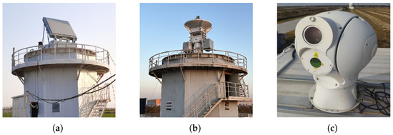
Figure 1.
Experimental equipment. (a) High-resolution phased-array scanning radar. (b) High-resolution tracking radar. (c) Optical imaging system.
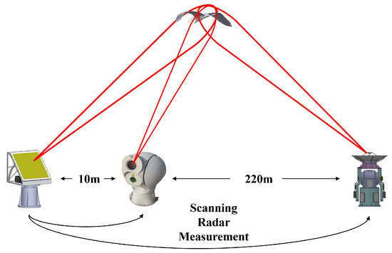
Figure 2.
Collaborative observation process for bird targets.

Table 1.
Radar parameters.
The bird detection experiment was conducted in Dongying, Shandong, in March 2022. A total of 60 sets of bird data were collected in the experiment, covering more than 10 species of bird targets. The collected bird targets and their associated sizes are shown in Table 2. To better illustrate the radar echo characteristics of bird targets, three bird targets of different body lengths (large, medium, and small) were selected for display, with the results shown in Figure 3. From the amplitude sequence and time–frequency spectrogram results, it can be observed that amplitude fluctuations caused by bird targets of different sizes vary. Additionally, due to differences in wing size, variations in micro-Doppler features on the time–frequency spectrogram were observed, with micro-Doppler characteristics of smaller birds being less pronounced than those of larger birds. Of course, the radar characteristics of birds of different sizes follow the same general pattern. The radar echo characteristics of bird targets were confirmed in the experiment, with significant fluctuations in the amplitude sequence and amplitude energy fluctuations caused by wing flapping reaching over 10 dB. The time–frequency analysis results consist of a main Doppler component caused by the bird’s body and a sinusoidal-like fluctuation component caused by wing flapping. Data with consistent radar characteristics from the samples collected by the high-resolution tracking radar were selected and identified as bird targets, with their radar echo results shown in Figure 4.
Table 2.
Bird parameters.
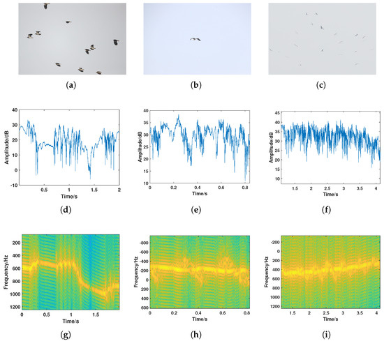
Figure 3.
Experimental results of optical–radar joint detection for typical bird species. (a–c): Optical image of the Northern Lapwing (a), Grey Heron (b), and Oriental Stork (c). (d–f): Radar amplitude sequence of the Northern Lapwing (d), Grey Heron (e), and Oriental Stork (f). (g–i): Radar time–frequency spectrogram of the Northern Lapwing (g), Grey Heron (h), and Oriental Stork (i).
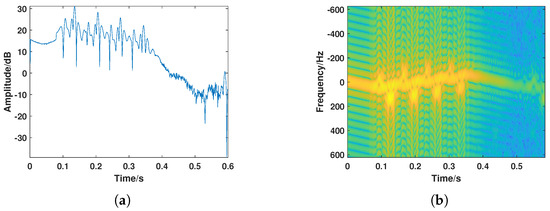
Figure 4.
A typical bird target. (a) Amplitude sequence. (b) Time–frequency spectrogram.
2.1.2. Comprehension of the Radar Echo Characteristics of Insects
Due to the small size of the insects, true target labels could not be obtained through long-range optical imagery. A mapping relationship was previously established by our team through the extraction of insect radar echo features, indirectly estimating the body length and weight of insects [36,37,38,39]. The radar observation data was compared with manually collected data from light trap to confirm the consistency between the radar-measured targets and aerial biological targets. Data from various insect species were analyzed, covering a wide range of body lengths and weights, including cotton bollworm, armyworm, corn borer, black cutworm, and other. The radar echoes of different insects exhibited high similarity, and a typical case of the cotton bollworm was used for detailed explanation.
On the night of 16–17 April 2023, 1095 cotton bollworms were captured, accounting for 57.62% of the total catch. The mass and length distributions of these cotton bollworms are shown in Figure 5a,b. Additionally, from 11 PM on 16 April to 5 AM on 17 April 2023, a total of 17,695 targets were detected by the radar, and the method was used to estimate the mass and length of the targets [36,37,38,39]. The estimated mass and length distributions are shown in Figure 5c,d, respectively. Approximately 67% of the insect morphological parameters matched those of the cotton bollworm. Furthermore, the full-polarization radar echoes from that date were manually filtered, with radar echo results showing strong convergence selected as typical insect radar echo characteristics. The typical radar echo results for insects from vertical observation mode are shown in Figure 6. The radar echo characteristics of insect targets were confirmed in the experiment. The range of amplitude sequence variations was smaller compared to birds, with amplitude changes caused by wing beats generally not exceeding 5 dB. The time–frequency spectrum typically consisted of a main Doppler component caused by the body, accompanied by micro-Doppler features with sawtooth-like fluctuations caused by wing beats. Additionally, due to the small amplitude fluctuations caused by the insect itself, when passing through the radar beam, modulation by the radar’s radiation pattern caused different amplitude variation trends.
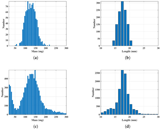
Figure 5.
Comparison of statistical results between the light trap and radar measurements. (a,b): Distribution of the mass (a) and length (b) of cotton bollworms captured by the light trap. (c,d): Distribution of the mass (c) and length (d) of insects measured by radar.

Figure 6.
A typical insect target. (a) Amplitude sequence. (b) Time–frequency spectrogram.
2.2. Biological Target Dataset Construction
The measured data were collected in Dongying, China, an area located along the migration routes of insects and birds, with a diverse range of species. Data were collected over several days, covering the migration seasons of various migratory pests and birds. Samples were taken during the migration season, and nighttime monitoring data from several days were selected to construct the database. The raw, unselected data exceeded 100,000 sets. A short-time Fourier transform (STFT) was performed on the targets, and amplitude sequences and time–frequency spectrogram results were generated for all targets. Based on the understanding of insect and bird radar echoes described in the previous section, the data categories were manually selected and classified, as shown in Table 3. During the selection and database construction process, three additional types of echo targets with distinct characteristics, apart from the typical insect and bird targets, were identified. These targets were separately extracted to ensure the completeness of the dataset. After these targets were fully extracted, the insect and bird data were balanced to a similar magnitude to ensure the equilibrium of the dataset for subsequent identification algorithms.
Table 3.
Dataset number for different types of airborne targets.
Next, the radar echo characteristics of the targets in the database will be elaborated in detail. A pattern database was built for the measured data based on target echo amplitude characteristics, micro-Doppler features, and wingbeat frequency biological parameters. The amplitude sequences and time–frequency spectrograms of various targets in the dataset are shown in Figure 7. A detailed description of the features of each category of targets is provided below.
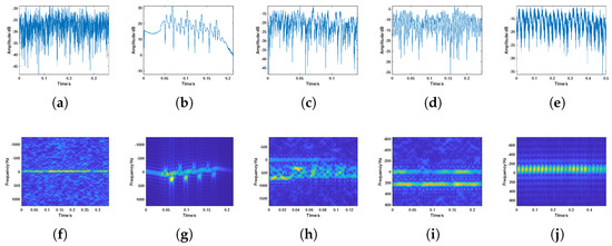
Figure 7.
Amplitude sequences and time–frequency spectrograms of various targets. (a–e): Amplitude sequence of (a) insect, (b) bird, (c) cluttered Doppler components, (d) multiple Doppler components, and (e) amplitude periodic fluctuations. (f–j): Time–frequency spectrograms of (a) insect, (b) bird, (c) cluttered Doppler components, (d) multiple Doppler components, and (e) amplitude periodic fluctuations.
(a) Insect: This type of target has a primary Doppler frequency that is relatively low, typically below 50 Hz, with minimal Doppler fluctuation. The echo amplitude variation generally does not exceed 10 dB.
(b) Bird: The Doppler and amplitude exhibit a wide range, with significant micro-Doppler fluctuations caused by bird wing flapping.
(c) Cluttered Doppler components (CD components): This type of target typically has a single primary Doppler component, but also exhibits relatively cluttered Doppler components.
(d) Multiple Doppler components (MulD components): The echoes of this type of target exhibit highly regular sinusoidal-like fluctuations, with multiple primary Doppler components in the time–frequency spectrogram.
(e) Amplitude periodic fluctuations (APF): The echoes of this type of target exhibit highly regular sinusoidal-like fluctuations with an amplitude of around 10 dB. The time–frequency spectrogram shows alternating bright and dark spots.
The typical insect and bird targets are supported by correctness experiments. However, to ensure the completeness of the aerial biological target dataset, the remaining three target categories were also selected. In the subsequent experimental section, these targets were analyzed either as three distinct categories or merged with other categories for algorithm performance evaluation. These echoes may represent insect targets with unique radar characteristics or targets mixed with certain clutter. During the dataset creation process, it was found that the overall proportion of these three categories was very low. Therefore, these targets have a minimal impact on the subsequent application of the insect and bird classification algorithm proposed in this paper.
2.3. Insect and Bird Separability Analysis
After the analysis and definition of aerial biological target characteristics were completed, further statistical analysis of the insect–bird data was conducted. This was performed to highlight the challenges in classifying aerial biological targets and, in turn, propose our targeted biological classification algorithm. The discussion focuses primarily on the echo amplitude, time-varying characteristics, and time–frequency characteristics of aerial biological targets.
2.3.1. Echo Amplitude
Generally, the RCS of bird targets is much larger than that of insect targets. However, due to the large size variation among aerial biological targets, many large bird targets can also be detected in the radar beam sidelobes. In such cases, the estimated RCS of bird targets may be underestimated, sometimes even comparable to that of insect targets. Therefore, after the manual selection of insect and bird data, their amplitude distributions were statistically analyzed. As shown in Figure 8, the overall amplitude distribution of bird targets is slightly larger than that of insect targets. However, there is still approximately a 70% overlap in the amplitude distribution between the two target types, making it impossible to use amplitude alone for the insect–bird classification task.
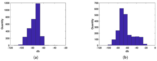
Figure 8.
Amplitude statistical distribution. (a) Insect. (b) Bird.
2.3.2. Time-Varying Characteristics
Insects and birds achieve flight by flapping their wings. Due to differences in their biological structures, the fluctuations in the radar echoes of most insect targets are caused by body vibrations. Bird targets, on the other hand, typically involve the interaction between the wings and body, which produces rapid fluctuations in radar echoes at different frequencies during wing flapping. Therefore, we statistically evaluated the rate of change in the radar echo signals for both target types. The evaluation method is as follows: first, the amplitude sequence of the insect and bird echoes is differentiated, and then the mean and variance of the differences for each target are calculated. As shown in Figure 9, the signal change rate for bird targets is slightly higher than that for insect targets, but the variance in the signal change is lower for birds, which is consistent with the conclusions drawn during the database construction.
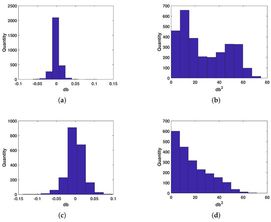
Figure 9.
Statistical distribution of signal change rate. (a,b) Statistical results of the mean (a) and variance (b) for insects. (c,d) Statistical results of the mean (c) and variance (d) for birds.
2.3.3. Time–Frequency Characteristics
The time–frequency analysis method used in this paper, the short-time Fourier transform (STFT), is effective in extracting the main Doppler and micro-Doppler components of different biological targets. The window length used in the short-time Fourier transform is consistent with the one used in the time–frequency spectrograms in the dataset creation, which is 24 ms. After obtaining the target time–frequency analysis results, the t-distributed stochastic neighbor embedding (t-SNE) [40] algorithm was applied to map the normalized time–frequency results with different window lengths into a two-dimensional space for dimensionality reduction. The resulting visualizations of the reduced dimensions are shown in Figure 10. The t-SNE is a dimensionality reduction method that represents the similarity of high-dimensional data as conditional probabilities and generates similar distributions in the low-dimensional space. When the two distributions are nearly identical, the projection of the high-dimensional data can be observed in the low-dimensional space. The x and y axes in Figure 10 represent the relative values after feature dimensionality reduction, used to characterize the relative distribution of various target types. They do not have specific physical meaning, so no coordinates are provided. Here, yellow represents bird targets, red represents insect targets, and the other three colors represent different target categories. It can be observed that insect and bird targets show some overlap in their distribution in the two-dimensional space, but also exhibit different clustering characteristics. This indicates that time–frequency spectrogram features can serve as effective features for insect and bird classification.
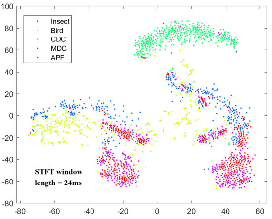
Figure 10.
t-SNE dimensionality reduction visualization result.
This subsection analyzes the echo amplitude, time-varying features, and time–frequency features of insects and birds. Due to the frequent occurrence of targets being detected in the radar sidelobes, the overlap of insect and bird echo amplitude features is large, making them difficult to use for insect and bird classification tasks. However, the echo variations of insects and birds exhibit different time-varying characteristics, which can be exploited by neural networks to extract high-dimensional features for classification. Additionally, the time–frequency spectrogram features of insects and birds show good separability in the reduced-dimensional 2D plane.
2.4. Analysis of the Transformation Results with Different Window Lengths
As analyzed earlier, this paper uses STFT to obtain the time–frequency spectrogram of biological targets. However, the window length of the STFT determines the time and frequency resolution of the time–frequency analysis results. For biological targets with different wing-beat frequencies, different window lengths are selected, resulting in different time–frequency analysis outcomes. Considering the wing-beat frequency range of aerial organisms is mainly from 5 to 80 Hz, a total of 14 window lengths, ranging from 4.8 ms to 46.4 ms with a 3.2 ms interval, were selected for short-time Fourier transform on the signal. The transformation results are shown in Figure 11. Due to limited image size, only the transformation results for eight window lengths are displayed. It can be observed that the micro-Doppler features in the time–frequency spectrograms of different window lengths show significant differences. To better quantify the differences in time–frequency spectrograms at different scales, the same method as before was used. The t-SNE algorithm was applied to map the normalized time–frequency analysis results with different window lengths to a two-dimensional space for dimensionality reduction, resulting in different dimensionality-reduced visualizations, as shown in Figure 12. Here, red represents insect targets, yellow represents bird targets, and the remaining three colors represent other targets. It can be seen that under different time–frequency analysis window lengths, the categories of targets exhibit different inter-class distance relationships. The mean Euclidean distance of the dimensionality-reduced features for insect and bird targets was calculated, and the Euclidean distances between each pair of insect and bird targets were averaged. The results are shown in Figure 13a, where it can be observed that the Euclidean distance differences of insect and bird features vary under different transformation window lengths. Additionally, the Pearson correlation coefficient of the features of a single target category under different window length transformations was also calculated. The correlation coefficient between the first window length transformation results and the other window length transformation results for each target was calculated, and the average value was taken. The results are shown in Figure 13b, where it can be seen that when the window length differences are large, the correlation coefficient is very low. This indicates that under different STFT window lengths, the time–frequency spectrograms represent different time–frequency resolution characteristics, which contribute inconsistently to the classification task. Therefore, it is necessary to introduce different STFT window lengths to improve the accuracy of target classification.
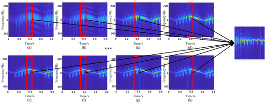
Figure 11.
Illustration of multi-scale time–frequency spectrogram concatenation. (a) The window length for the STFT is 4.8 ms. (b) The window length for the STFT is 8 ms. (c) The window length for the STFT is 11.2 ms. (d) The window length for the STFT is 14.4 ms. (e) The window length for the STFT is 36.8 ms. (f) The window length for the STFT is 40 ms. (g) The window length for the STFT is 43.2 ms. (h) The window length for the STFT is 46.4 ms.
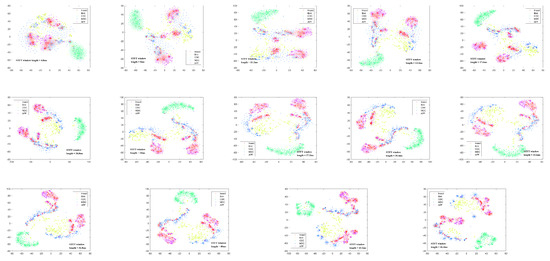
Figure 12.
t-SNE dimensionality reduction visualization results for 14 window lengths ranging from 4.8 ms to 46.4 ms with an interval of 3.2 ms.
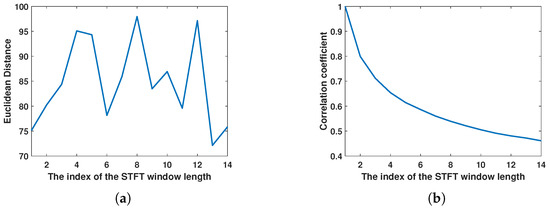
Figure 13.
Analysis of window length features in short-time Fourier transform. (a) Euclidean distance between insect and bird features. (b) Pearson correlation coefficient for the same type of target.
2.5. Data Preprocessing
After the dataset was constructed, the raw data were preprocessed and specifically normalized. The preprocessing mainly consisted of two parts: the processing of the amplitude sequence and the time–frequency spectrogram. The specific operations will be elaborated on in the following sections.
2.5.1. Processing of the Amplitude Sequence
Amplitude sequence normalization mainly consists of two steps: intensity normalization and length uniformity. Traditional intensity normalization generally involves subtracting the minimum value from each point in the sequence, then dividing by the difference between the maximum and minimum values, ensuring the normalized data range is between 0 and 1. However, due to the large differences in the fluctuation characteristics of insects and birds, using the above method would artificially distort the relative fluctuation characteristics of the amplitude sequence. Therefore, the amplitude sequence is directly divided by its maximum value as the normalization result. Additionally, since the lengths of the data vary, length uniformity is achieved by downsampling or upsampling the data to normalize it to a sequence of length 512.
2.5.2. Processing of the Time–Frequency Spectrogram
Due to the large pulse repetition frequency of the radar, a wide Doppler range is covered. Considering that the proportion of valid target information in the time–frequency spectrogram is relatively low, directly inputting the spectrogram into subsequent algorithms would introduce significant redundant information. Therefore, frequency dimension scale normalization was applied to the time–frequency spectrogram. The procedure is as follows: the instantaneous frequency sequence was extracted, and the average value of the instantaneous frequency sequence was used as the frequency center for the normalized image, with a certain frequency range above and below it to define the valid image range. At low signal-to-noise ratios, this can lead to outliers in the extracted instantaneous Doppler frequencies. However, considering the large Doppler span of bird targets, removing outliers might incorrectly discard the micro-Doppler features of bird targets. A slightly larger frequency range was chosen to ensure full coverage of the Doppler features of biological targets. Based on empirical statistics, a frequency range of 400 Hz above and below the frequency center was selected to define the valid image range. The normalization results are shown in Figure 14. Furthermore, the time–frequency spectrograms were downsampled to a size of 112 × 112, completing the normalization of each spectrogram.
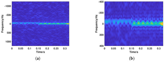
Figure 14.
Normalization results of the time–frequency spectrogram. (a) Original time–frequency spectrogram. (b) Time–frequency spectrogram after normalization.
In the previous analysis, the differences in time–frequency spectrograms at different scales were pointed out. To better mine the target micro-Doppler features in the time–frequency spectrogram, frequency and time features were considered separately. This also required further processing of the 14 normalized time–frequency spectrograms obtained. A time window of 8 points was sequentially extracted from each time–frequency spectrogram and reassembled into 14 new frequency feature maps. This resulted in feature maps representing the micro-Doppler characteristics of the target at different frequency resolutions within the same time window. By following this process, 14 reassembled frequency feature maps were ultimately obtained. It is believed that the new feature maps better reflect the changes in micro-Doppler characteristics caused by different frequency resolutions of the target at the same time. The stitching method is shown in Figure 11.
3. Biological Target Classification Algorithm Based on Multi-Scale Time–Frequency Deep Feature Fusion Network
To maximize the utilization of different target features and achieve more accurate classification results, the multi-scale time–frequency deep feature fusion network (MSTFF-Net) is proposed for aerial weak biological target classification. The structure of MSTFF-Net is shown in Figure 15. The MSTFF-Net structure mainly includes the time–frequency feature extraction module, amplitude sequence feature extraction module, adaptive feature fusion attention module, and classification part. The time–frequency feature extraction module performs hierarchical feature extraction on the proposed new time–frequency feature maps in both the frequency and time domains. The amplitude sequence feature extraction module is used to extract the characteristic fluctuation features from the target amplitude sequence. The adaptive feature fusion attention module adjusts the feature dimensions and introduces an attention mechanism to further focus on the effective features, thereby improving classification accuracy. The classification module performs probability mapping on the fused high-dimensional features to obtain the target class. The structure of these four components will be described in detail in the following sections.
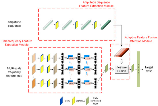
Figure 15.
Overall framework of the multi-scale time–frequency deep feature fusion classification network.
3.1. Amplitude Sequence Feature Extraction Module (ASEM)
The amplitude sequence data are input into the amplitude sequence feature extraction module to obtain a deep representation of amplitude-related features. The amplitude sequence contains useful information reflecting target dynamics. Specifically, it includes vibration signals from non-rigid biological targets and periodic changes caused by body posture variation. A Convolutional Neural Network (CNN) [41] is employed to extract the deep features of the target’s amplitude sequence. For a series of amplitude sequences of size , where H denotes the length of each amplitude sequence. Subsequently, for a typical multi-channel convolution operation, the convolution kernel is of size . The output feature maps for all channels can be represented as:
where V represents the size of the convolution kernel, is the amplitude value of the subsequence at position j in the amplitude sequence, and is the convolution kernel weight at position j in the amplitude sequence.
A typical CNN consists of several convolutional layers, pooling layers, fully connected layers, and an output layer. First, the convolutional layers extract local features from the magnitude sequence by sliding convolutional kernels, with each convolutional layer containing multiple kernels with different weights. Subsequently, the pooling layers, located after the convolutional layers, reduce the computational load of the network by suppressing redundant information in the extracted features. Finally, the deep features are passed to the output layer to predict the target class. Given that complex network structures may lead to difficulties in convergence, the magnitude sequence module uses a ResNet18 [42] to extract deep magnitude features. The structure of the ResNet18 is shown in Figure 16.
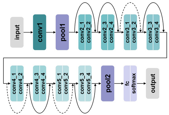
Figure 16.
The structure of amplitude sequence feature extraction module.
3.2. Time–Frequency Feature Extraction Module (MTEM)
In traditional airborne target classification research, the micro-motion features of the target are widely utilized, with the STFT commonly used to obtain the target’s time–frequency spectrogram. A strong correlation between the target’s micro-motion features and the window length used in the STFT was found in the previous data analysis. It is believed that optimal results cannot be achieved by simply obtaining a time–frequency spectrogram using a single window length and training the network on it. Therefore, STFT is performed with different window lengths to obtain time–frequency spectrograms at different resolution scales, which are then reorganized and stitched according to certain rules. The specific operations related to this have been detailed in the data preprocessing subsection of the previous text. The 14 reassembled feature maps are referred to as frequency feature maps, which better reflect the micro-Doppler characteristic changes caused by different frequency resolutions of the target at the same time. The frequency feature map data are first processed in parallel by the multi-scale frequency feature extraction module to obtain a joint feature representation. By performing multi-scale information learning in the multi-scale frequency feature extraction module, the extracted joint features exhibit greater discriminative power than traditional single-scale deep features. Therefore, superior classification results can be achieved. The designed multi-scale feature extraction module is based on a residual block structure. It consists of five convolutional modules, with the first convolutional layer using a 7 × 7 kernel size. Given the large size of the original image and the fact that the classification task primarily involves time–frequency spectrogram patterns, a large kernel is used for downsampling the input to reduce the overall computational load of the network. The subsequent four residual convolutional blocks have the same structure, each consisting of four convolutional layers with a 3 × 3 kernel size. Residual connections are used to mitigate overfitting and the vanishing gradient problem. Additionally, batch normalization and activation functions are applied in each convolutional block.
After feature extraction by the four residual convolutional blocks is completed, the outputs of the first three residual blocks are passed through 1 × 1 channel convolutional blocks for channel adjustment. On the one hand, activation functions are added during the channel adjustment process to further enhance the non-linearity of the features. On the other hand, the number of channels in the four residual blocks is kept consistent to facilitate subsequent feature fusion. After the channel adjustment is completed, the outputs of the adjusted four residual blocks are uniformly passed into the adaptive sliding window pooling module to adjust the size of the feature maps. Finally, the four feature maps are concatenated to complete the multi-scale frequency feature extraction. The specific structure of the multi-scale frequency feature extraction module is shown in Figure 17.
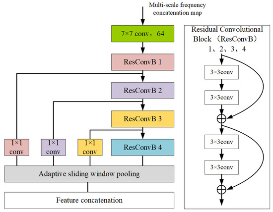
Figure 17.
Multi-scale frequency feature extraction module.
Inspired by the ability of Recurrent Neural Network (RNN) [43] to model contextual dependencies in time series, after deep frequency feature extraction is completed, the extraction of deep temporal features is considered. The extracted deep frequency features are sequentially flattened into one-dimensional feature vectors, and an RNN is employed to extract deep temporal features. In traditional RNN, the output from the previous time step is fed back and used as additional input for the current state. It is capable of learning contextual information and maintaining a "memory" of the entire sequence. However, traditional RNN cannot handle long-period time series due to the vanishing gradient problem.
Long-term memory is the key distinction between LSTM [44] networks and traditional RNN networks. Traditional RNN networks use only short-term memory to connect adjacent RNN units. Therefore, when an RNN network needs to handle sequences with long-term dependencies, the network depth must be increased, which may lead to the vanishing gradient problem. LSTM networks introduce the concept of long-term memory, which is propagated along the time axis, with only linear operations (such as multiplication and addition) performed during the propagation. As a result, significant changes are not introduced, and it serves as a "conveyor belt" for long-term information. At the same time, is able to provide each LSTM unit with information from the previous time steps, thereby eliminating the need to significantly increase network depth during long sequence training, thus avoiding the vanishing gradient problem.
The one-dimensional frequency features at different time steps are input into the stacked Bi-LSTM module shown in Figure 18. Specifically, the Bi-LSTM module used in the MTEM consists of two stacked Bi-LSTM layers, each with 128 hidden units in both forward and backward directions. Following the Bi-LSTM layers, we apply a dropout layer with a dropout rate of 0.3 to reduce overfitting. The output of the module is the deep temporal features of the time–frequency spectrogram, as the recurrent network has already captured the temporal dependencies. LSTMs can be optimized using the back propagation through time (BPTT) algorithm [45]. Based on BPTT, the recurrent network can be unfolded into a multi-layer feedforward deep network, and traditional back propagation (BP) algorithms can be used to optimize the LSTM parameters.
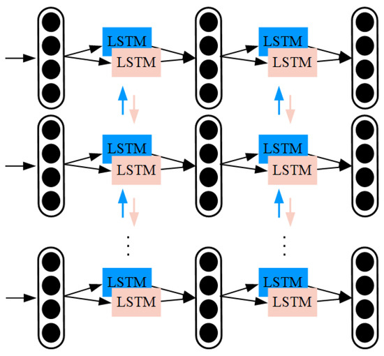
Figure 18.
Temporal feature extraction module.
3.3. Adaptive Feature Fusion Attention Module (FFAM)
After the deep feature extraction of amplitude sequences and time–frequency features is completed, the two types of features are fused for the final target classification task. The introduction of the adaptive feature fusion attention module aims to capture the correlations and differences between different types of features. It effectively eliminates information discrepancies, performs feature fusion, and suppresses channels with low relevance to the classification task to enhance network performance. Two feature fusion modules, namely the enhanced pooling module and the channel spatial attention module, are introduced in this paper, and each module will be discussed in detail in the following sections.
3.3.1. Enhanced Pooling Module
Average pooling and global max pooling are employed to obtain deep features that are more sensitive to the target texture and background, respectively. These two types of deep features are then combined to obtain a more comprehensive feature representation. The specific operation is shown in Figure 19a.
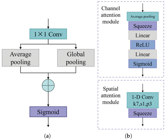
Figure 19.
Architecture of the feature fusion attention module. (a) Enhanced pooling module. (b) Channel spatial attention module.
3.3.2. Channel Spatial Attention Module
The channel spatial attention module extracts information from each feature channel separately, without considering the potential of feature correlations to improve target classification accuracy. To overcome this limitation, channel attention [46] and spatial attention [47] mechanisms are introduced separately and concatenated to further enhance the feature fusion capability. The channel spatial attention module is shown in Figure 19b.
Given an input feature map , the channel spatial attention module computes a 1D channel attention matrix and a 1D spatial attention matrix ,
where ⊗ represents element-wise multiplication and denotes the final output of the channel spatial attention module. The output of the channel attention module can be expressed as follows.
where represents the Sigmoid function, denotes the fully connected layer, signifies the compression operation, and indicates the adaptive average pooling operation. The output of the spatial attention module can be expressed as follows,
where represents the convolution module.
The introduction of the channel spatial attention module is motivated by the fact that the amplitude sequences and multi-scale time–frequency spectra of aerial biological targets often exhibit complex motion characteristics and differentiated amplitude variations caused by different target sizes, which contain rich target information. The channel attention feature map in the channel spatial attention module mainly focuses on the relationships between different channels. By learning to adjust the weights of each channel, the useful feature channels are enhanced, and the channels with low relevance are suppressed, thereby improving the channel characteristics of the aerial target features. On the other hand, the spatial attention feature map learns the importance of different positions within the features, thereby enhancing the learning of spatial contextual characteristics. Therefore, the introduction of the channel spatial attention module allows for better attention to the correlated features of the amplitude sequences and time–frequency spectra of aerial biological targets, thus improving the accuracy of aerial target classification.
3.3.3. Feature Fusion Strategy
The proposed feature fusion strategy primarily involves fusing the single feature output from the enhanced pooling module with the interactive features output by the channel spatial attention module, as shown in Figure 20. The entire feature fusion strategy can be expressed as follows,
where represents the feature map of the enhanced pooling module, denotes the deep features of the amplitude sequence, refers to the multi-scale time–frequency deep features, represents the feature map of the channel spatial attention module, and © indicates the concatenation operation. The final fused feature output is obtained by summing the output attention features.
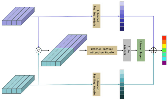
Figure 20.
Architecture of feature fusion attention module.
Finally, the output of the feature fusion attention module is input into the classifier module for aerial target classification.
3.4. The Training of MSTFF-Net
For training the MSTFF-Net network, the normalized time–frequency spectrogram and amplitude sequence are first input into the time–frequency multi-scale feature extraction module and the amplitude sequence temporal feature extraction module, respectively, where multi-scale time–frequency deep features and amplitude sequence temporal deep features are extracted. Subsequently, through the feature adjustment module, the multi-scale time–frequency deep features and amplitude sequence temporal deep features are normalized and then concatenated, before being passed into the adaptive feature fusion attention module, which produces the fused features. The fused features are then processed through a fully connected layer to obtain the output feature vector . Finally, the feature vector is input into the softmax classification function to obtain the probability distribution for each class. The calculation of the probability distribution is shown below,
where C represents the total number of classes.
After obtaining the class probability distribution, the cross-entropy loss function is used to compute the loss based on the probability distribution obtained in each training iteration and the sample labels. To minimize the training loss, the Adam optimizer is used to update the MSTFF-Net parameters through the backpropagation process. When the loss no longer decreases and stabilizes, the parameter updates are complete, signifying that MSTFF-Net has finished training.
During the network prediction process, both the target time–frequency spectrogram and the amplitude sequence inputs follow the same path as during training to predict the class labels, with the label determined by the maximum probability output from the softmax function.
4. Experiments
This section presents experiments to evaluate the classification performance of the proposed network structure. First, the experimental dataset, experimental setup, and evaluation metrics are introduced. The effectiveness of the proposed model was verified from three perspectives. First, the confusion matrices for the three-class and five-class network classifications are presented. Next, the contribution of each module in the proposed network to the overall classification performance is analyzed. Finally, a comparison of the classification performance with traditional methods in the field is provided.
4.1. Data and Experimental Description
The training and testing data were collected by the team, using the five categories described in Section 2 as the experimental dataset, with a total of 7326 data slices. During the algorithm experiments, experiments with three categories (by combining the remaining three target classes into "other") was conducted. For each target class, 1000 samples were selected as the training set. The remaining data were used as the test set. The number of targets of different types is shown in Table 3.
The proposed network architecture is implemented using the NVIDIA RTX A6000 GPU, sourced from PNY Technologies, headquartered in Parsippany-Troy Hills, New Jersey, USA. The implementation utilizes the PyTorch framework, version 1.11.0+cu113, which is compatible with the CUDA 12.4 toolkit. The Adam optimizer with a learning rate of 1e-5 and momentum of 0.9 is used to update the parameters of the proposed network. The training period is set to 1000 epochs, with a learning rate of 0.001. The learning rate is halved after 10 epochs of no loss decrease, and the batch size is set to 16.
4.2. Classification Performance Evaluation Metrics
In this paper, accuracy, precision, recall, and F1 score are used as evaluation metrics to quantify the classification performance of the proposed structure. A higher score for each metric indicates better classification performance. To minimize experimental errors, all training processes are repeated ten times, and the results are averaged.
where TP represents the positive samples predicted as the positive class, TN represents the negative samples predicted as the negative class, FN represents the positive samples predicted as the negative class, and FP represents the negative samples predicted as the positive class.
4.3. Network Test Results
Considering the imbalance in the sample sizes across categories, and the fact that in practical applications we are more concerned with the number of typical insect and bird targets, we validated the classification performance for insects, birds, and other targets using a large dataset. The three-class confusion matrix is shown in Table 4. The results show that the classification accuracy for the three-class classification reached 94.0%. There were fewer misclassifications between insects and birds. Some insect targets were misclassified as other targets. Considering that in practical situations, the number of insect targets far exceeds the number of bird targets, this algorithm exhibits relatively few misclassifications between insects and birds. It can effectively describe the quantity and spatiotemporal distribution of insects and birds.
Table 4.
Three-class confusion matrix for aerial targets.
4.4. Ablation Experiment Analysis
In this section, ablation experiment analysis is conducted on each feature extraction module and the overall structure.
4.4.1. Ablation Experiment of the Structure
Each module of the proposed model plays a crucial role in the aerial target classification task. This subsection will conduct an ablation analysis of the proposed modules to demonstrate their effectiveness. The quantitative results of the ablation experiments are shown in Table 5. In the table, a checkmark indicates that the corresponding module and input data were used, a dash indicates that the data used did not require the corresponding module, and a cross indicates that the corresponding module was not used. Ablation experiments were conducted from two perspectives: input ablation and module ablation. It can be observed that using only amplitude sequence information or multi-scale time–frequency information does not achieve satisfactory classification performance. When both features are used, the performance improves by 24.4% and 3.6% compared to using each feature individually. However, the two features were not effectively fused. After introducing the fusion attention module proposed by us, the classification performance for aerial biological targets further improved by 4%, validating the effectiveness of our proposed algorithm.
Table 5.
Module ablation experiments.
4.4.2. Analysis of the Amplitude Sequence Feature Extraction Module
It can be seen from previous experiments that the introduction of amplitude sequence inputs can improve the classification accuracy of airborne biological targets. Based on Convolutional Neural Networks (ResNet-18), Recurrent Neural Networks (Bi-LSTM), and Convolutional Long Short-Term Memory Networks (Conv-LSTM), three feature extraction modules are designed. The impact of different feature extraction modules on the classification results of amplitude sequence inputs is verified, and the quantitative analysis results are presented in Table 6. The classification performance using ResNet-18 is significantly better than the other two methods, with an improvement of 6.9% and 2.2% in classification accuracy compared to Bi-LSTM and Conv-LSTM, respectively.
Table 6.
Classification comparison results of the amplitude sequence feature extraction modules.
4.4.3. Analysis of the Multi-Scale Time–Frequency Feature Extraction Module
As mentioned earlier, a single time–frequency spectrum is not used as the input in this paper. Instead, multi-scale window lengths are first used for short-time Fourier transforms, and then segments from the same time window are extracted and concatenated to form frequency features. After extracting deep frequency features, deep temporal sequence features of airborne biological targets are further extracted. In the process of considering how to better use multi-scale time–frequency features, different feature extraction structures are designed, and various feature interaction strategies are applied to extract the optimal multi-scale time–frequency features. For single time–frequency spectrogram module, a single scale-transformed time–frequency spectrum is used, normalized, and input as a 1 × 112 × 112 matrix, which is then processed through a series of Convolutional Neural Network modules to obtain deep time–frequency features. This is referred to as the single time–frequency spectrogram structure in these subsections. For multiple time–frequency spectrogram module, after obtaining 14 time–frequency spectra from different scale transformations, 14 parallel channels are used to extract deep target features. After feature extraction in each residual block, a 1 × 1 convolutional block is used for interactive learning across the 14 channels, which are then added back to each respective channel, ultimately resulting in deep time–frequency features. This is referred to as the multiple time–frequency spectrogram structure in this subsection. The third structure is the time–frequency deep feature extraction module proposed in this paper. To ensure fairness in the evaluation method, the convolutional modules of all three structures use the designed residual concatenated convolution modules. The quantitative results of different time–frequency feature extraction modules are presented in Table 7.
Table 7.
Classification comparison results of the time–frequency feature extraction modules.
4.4.4. Analysis of the Feature Fusion Module
The feature fusion module is designed to integrate deep amplitude features and time–frequency features. Optimizations are made based on channel attention and spatial attention, and a new feature fusion mechanism is designed. In this section, the algorithm performance is compared with three attention mechanisms, which include the channel attention mechanism, spatial attention mechanism, and channel–space attention mechanism. The quantitative results of different attention mechanism feature fusion modules are shown in Table 8. It can be observed that the proposed feature fusion attention module demonstrates a significant performance improvement in classification compared to other fusion mechanisms. The use of the channel–space attention mechanism results in more than a 1% improvement in classification performance compared to using either attention mechanism individually. This may be because the model requires the introduction of attention mechanisms for both channel and spatial features to enhance its ability to focus on relevant information. The proposed structure shows a 1.3% improvement in classification accuracy compared to the channel–space attention mechanism. This may be because the channel–space attention mechanism used only focuses on single amplitude features or multi-scale time–frequency features, without considering the interaction between the two feature types. The proposed structure, however, is capable of effectively learning interaction features, further enhancing the classification performance of the fusion attention module.
Table 8.
Classification results of the feature fusion modules.
4.5. Performance Comparison Analysis with Traditional Methods
Traditional biological target classification methods mostly use a single feature of the target (e.g., amplitude sequence, time–frequency transformation) as the input feature. This subsection will introduce and compare the performance of two mainstream airborne target classification methods with the approach proposed in this paper. Considering the practical applications, the number of insect targets is significantly higher than that of bird and other targets. The evaluation metrics in this section are consistent with those used in previous sections, and will calculate the overall accuracy, as well as the precision, recall, and F1 score for insect targets to evaluate the algorithm. All results are presented in Table 9.
Table 9.
Classification results of the dataset using different methods.
(1) Some scholars extract features from the amplitude sequences or time–frequency spectra of airborne biological targets to describe the target’s amplitude fluctuations, such as cepstral coefficients, linear predictive coding coefficients, amplitude perturbation, and main Doppler frequency. These features are then combined with machine learning methods, such as random forests, to classify airborne biological targets.
(2) Some scholars have introduced neural networks for airborne biological target classification, typically using time–frequency spectra or amplitude sequences as inputs. This subsection compares the performance of methods using time–frequency map inputs and a series of popular networks. The networks include AlexNet, Bidirectional Long Short-Term Memory network (Bi-LSTM), Visual Geometry Group series (VGG-11), and Residual Network (ResNet-18).
5. Conclusions
In this paper, an intelligent classification method based on MSTFF-Net is proposed for airborne biological target classification. It mainly consists of three components: the first is the amplitude sequence feature extraction module for extracting features from the dynamic information of target echoes, the second is the target dynamic feature extraction module for extracting features from the reconstructed multi-scale time–frequency maps, and the third is the feature fusion attention module, which captures effective features of both types of information through the attention mechanism. A more complete airborne target dataset is established in this paper, with ground truth labels created for observation data across all periods. The algorithm’s effectiveness is validated using the self-built dataset. Although the proposed network shows satisfactory classification performance for airborne biological targets, future research should focus on further expanding the dataset to obtain a more robust model and confirming the natural categories of targets for subsequent scientific analysis and research.
Author Contributions
Conceptualization, L.W. and W.L.; methodology, L.W., R.W., W.L., J.W., Y.Y. and C.H.; investigation, L.W.; resources, R.W., W.L. and C.H.; data curation, L.W., W.L., J.W., Y.Y. and C.H.; writing—original draft preparation, L.W.; writing—review and editing, R.W., W.L., J.W. and Y.Y. All authors have read and agreed to the published version of the manuscript.
Funding
This work was supported in part by the National Natural Science Foundation of China under Grant 62201049, in part by the Special Fund for Research on National Major Research Instruments under Grant 31727901, and in part by the Shandong Provincial Natural Science Foundation, China (ZR2022QF073).
Data Availability Statement
In this paper, we have established an insect and bird dataset based on a high-resolution radar system. However, due to the difficulty in data acquisition, we do not plan to make the dataset publicly available at this time.
Acknowledgments
During the preparation of this manuscript/study, the authors used GPT for the purposes of English grammar proofreading. The authors have reviewed and edited the output and take full responsibility for the content of this publication.
Conflicts of Interest
The authors declare no conflicts of interest.
Abbreviations
The following abbreviations are used in this manuscript:
| MSTFF-Net | multi-scale time–frequency deep feature fusion network |
| RCS | radar cross section |
| CNN | convolution neural network |
| STFT | short-time Fourier transform |
| t-SNE | t-distributed stochastic neighbor embedding |
| RNN | Recurrent Neural Network |
| LSTM | Long Short-Term Memory |
| BPTT | back propagation through time |
| BP | back propagation |
References
- Jonzén, N.; Lindén, A.; Ergon, T.; Knudsen, E.; Vik, J.O.; Rubolini, D.; Piacentini, D.; Brinch, C.; Spina, F.; Karlsson, L.; et al. Rapid Advance of Spring Arrival Dates in Long-Distance Migratory Birds. Science 2006, 312, 1959–1961. [Google Scholar] [CrossRef] [PubMed]
- Robinson, R.A.; Crick, H.Q.P.; Learmonth, J.A.; Maclean, I.M.D.; Thomas, C.D.; Bairlein, F.; Forchhammer, M.C.; Francis, C.M.; Gill, J.A.; Godley, B.J.; et al. Travelling through a warming world: Climate change and migratory species. Endanger. Species Res. 2009, 7, 87–99. [Google Scholar] [CrossRef]
- Bauer, S.; Hoye, B.J. Migratory Animals Couple Biodiversity and Ecosystem Functioning Worldwide. Science 2014, 344, 1242552. [Google Scholar] [CrossRef]
- Zrnic, D.; Ryzhkov, A. Observations of insects and birds with a polarimetric radar. IEEE Trans. Geosci. Remote Sens. 1998, 36, 661–668. [Google Scholar] [CrossRef]
- Gauthreaux, S.A., Jr. The Flight Behavior of Migrating Birds in Changing Wind Fields: Radar and Visual Analyses1. Am. Zool. 2015, 31, 187–204. [Google Scholar] [CrossRef]
- Vaughn, C. Birds and insects as radar targets: A review. Proc. IEEE 1985, 73, 205–227. [Google Scholar] [CrossRef]
- Wainwright, C.E.; Stepanian, P.M.; Reynolds, D.R.; Reynolds, A.M. The movement of small insects in the convective boundary layer: Linking patterns to processes. Sci. Rep. 2017, 7, 5438. [Google Scholar] [CrossRef]
- Smith, A.D.; Reynolds, D.R.; Riley, J.R. The use of vertical-looking radar to continuously monitor the insect fauna flying at altitude over southern England. Bull. Entomol. Res. 2000, 90, 265–277. [Google Scholar] [CrossRef]
- Chapman, J.W.; Reynolds, D.R.; Mouritsen, H.; Hill, J.K.; Riley, J.R.; Sivell, D.; Smith, A.D.; Woiwod, I.P. Wind Selection and Drift Compensation Optimize Migratory Pathways in a High-Flying Moth. Curr. Biol. 2008, 18, 514–518. [Google Scholar] [CrossRef]
- Chapman, J.W.; Nesbit, R.L.; Burgin, L.E.; Reynolds, D.R.; Smith, A.D.; Middleton, D.R.; Hill, J.K. Flight Orientation Behaviors Promote Optimal Migration Trajectories in High-Flying Insects. Science 2010, 327, 682–685. [Google Scholar] [CrossRef]
- Alerstam, T.; Chapman, J.W.; Bäckman, J.; Smith, A.D.; Karlsson, H.; Nilsson, C.; Reynolds, D.R.; Klaassen, R.H.; Hill, J.K. Convergent patterns of long-distance nocturnal migration in noctuid moths and passerine birds. Proc. Biol. Sci. 2011, 278, 3074–3080. [Google Scholar] [CrossRef] [PubMed]
- Riley, J.R. Collective orientation in night-flying insects. Nature 1975, 253, 113–114. [Google Scholar] [CrossRef]
- Chapman, J.W.; Nilsson, C.; Lim, K.S.; Bäckman, J.; Reynolds, D.R.; Alerstam, T. Adaptive strategies in nocturnally migrating insects and songbirds: Contrasting responses to wind. J. Anim. Ecol. 2016, 85, 115–124. [Google Scholar] [CrossRef]
- Richter, J.H.; Jensen, D.R.; Noonkester, V.R.; Kreasky, J.B.; Stimmann, M.W.; Wolf, W.W. Remote Radar Sensing: Atmospheric Structure and Insects. Science 1973, 180, 1176–1178. [Google Scholar] [CrossRef]
- Reynolds, D.R.; Chapman, J.W.; Edwards, A.S.; Smith, A.D.; Wood, C.R.; Barlow, J.F.; Woiwod, I.P. Radar studies of the vertical distribution of insects migrating over southern Britain: The influence of temperature inversions on nocturnal layer concentrations. Bull. Entomol. Res. 2005, 95, 259–274. [Google Scholar] [CrossRef]
- Gauthreaux, J.S.A. Bird Migration: Methodologies and Major Research Trajectories (1945-1995). The Condor 1996, 98, 442–453. [Google Scholar] [CrossRef]
- Henningsson, P.; Karlsson, H.; Bäckman, J.; Alerstam, T.; Hedenström, A. Flight speeds of swifts (Apus apus): Seasonal differences smaller than expected. Proc. R. Soc. Biol. Sci. 2009, 276, 2395–2401. [Google Scholar] [CrossRef]
- Karlsson, H.; Nilsson, C.; Bäckman, J.; Alerstam, T. Nocturnal passerine migrants fly faster in spring than in autumn: A test of the time minimization hypothesis. Anim. Behav. 2012, 83, 87–93. [Google Scholar] [CrossRef]
- Grönroos, J.; Green, M.; Alerstam, T. To fly or not to fly depending on winds: Shorebird migration in different seasonal wind regimes. Anim. Behav. 2012, 83, 1449–1457. [Google Scholar] [CrossRef]
- Shi, X.; Schmid, B.; Tschanz, P.; Segelbacher, G.; Liechti, F. Seasonal Trends in Movement Patterns of Birds and Insects Aloft Simultaneously Recorded by Radar. Remote Sens. 2021, 13, 1839. [Google Scholar] [CrossRef]
- Hu, C.; Cui, K.; Wang, R.; Long, T.; Ma, S.; Wu, K. A Retrieval Method of Vertical Profiles of Reflectivity for Migratory Animals Using Weather Radar. IEEE Trans. Geosci. Remote Sens. 2020, 58, 1030–1040. [Google Scholar] [CrossRef]
- Horton, K.G.; La Sorte, F.A.; Sheldon, D.; Lin, T.Y.; Winner, K.; Bernstein, G.; Maji, S.; Hochachka, W.M.; Farnsworth, A. Phenology of nocturnal avian migration has shifted at the continental scale. Nat. Clim. Change 2020, 10, 63–68. [Google Scholar] [CrossRef]
- Dokter, A.M.; Farnsworth, A.; Fink, D.; Ruiz-Gutierrez, V.; Hochachka, W.M.; La Sorte, F.A.; Robinson, O.J.; Rosenberg, K.V.; Kelling, S. Seasonal abundance and survival of North America’s migratory avifauna determined by weather radar. Nat. Ecol. Evol. 2018, 2, 1603–1609. [Google Scholar] [CrossRef] [PubMed]
- Dokter, A.; Desmet, P.; Spaaks, J.; Hoey, S.; Veen, L.; Verlinden, L.; Nilsson, C.; Haase, G.; Leijnse, H.; Farnsworth, A.; et al. bioRad: Biological analysis and visualization of weather radar data. Ecography 2018, 42, 852–860. [Google Scholar] [CrossRef]
- Dokter, A.M.; Liechti, F.; Stark, H.; Delobbe, L.; Tabary, P.; Holleman, I. Bird migration flight altitudes studied by a network of operational weather radars. J. R. Soc. Interface 2011, 8, 30–43. [Google Scholar] [CrossRef]
- Gauthreaux, S.; Diehl, R. Discrimination of Biological Scatterers in Polarimetric Weather Radar Data: Opportunities and Challenges. Remote Sens. 2020, 12, 545. [Google Scholar] [CrossRef]
- Jatau, P.; Melnikov, V.; Yu, T.Y. A Machine Learning Approach for Classifying Bird and Insect Radar Echoes with S-Band Polarimetric Weather Radar. J. Atmos. Ocean. Technol. 2021, 38, 1797–1812. [Google Scholar] [CrossRef]
- Sun, Z.; Hu, C.; Cui, K.; Wang, R.; Ding, M.; Yan, Z.; Wu, D. Extracting Bird and Insect Migration Echoes From Single-Polarization Weather Radar Data Using Semi-Supervised Learning. IEEE Trans. Geosci. Remote Sens. 2024, 62, 5216612. [Google Scholar] [CrossRef]
- Russell, K.R.; Gauthreaux, S.A. Use of weather radar to characterize movements of roosting purple martins. Wildl. Soc. Bull. 1998, 26, 5–16. [Google Scholar]
- Lilliendahl, K.; Solmundsson, J.; Gudmundsson, G.A.; Taylor, L. Can Surveillance Radar be used to Monitor the Foraging Distribution of Colonially Breeding Alcids? Condor 2003, 105, 145–150. [Google Scholar] [CrossRef]
- Bloch, R.; Bruderer, B. The air speed of migrating birds and its relationship to the wind. Behavioral Ecology and Sociobiology 1982, 11, 19–24. [Google Scholar] [CrossRef]
- Feng, H.Q.; Zhang, Y.H.; Wu, K.M.; Cheng, D.F.; Guo, Y.Y. Nocturnal windborne migration of ground beetles, particularly Pseudoophonus griseus (Coleoptera: Carabidae), in China. Agric. For. Entomol. 2007, 9, 103–113. [Google Scholar] [CrossRef]
- Hamer, T.E.; Schuster, S.; Meekins, D. Radar as a tool for monitoring Xantus’s Murrelet populations. Mar. Ornithol. 2005, 33, 139–146. [Google Scholar] [CrossRef]
- Schmaljohann, H.; Liechti, F.; BÄchler, E.; Steuri, T.; Bruderer, B. Quantification of bird migration by radar—A detection probability problem. Ibis 2008, 150, 342–355. [Google Scholar] [CrossRef]
- Zaugg, S.; Saporta, G.; van Loon, E.; Schmaljohann, H.; Liechti, F. Automatic identification of bird targets with radar via patterns produced by wing flapping. J. R. Soc. Interface 2008, 5, 1041–1053. [Google Scholar] [CrossRef]
- Wang, R.; Wang, J.; Li, W.; Li, M.; Zhang, F.; Hu, C. Robust Estimation of Insect Morphological Parameters for Entomological Radar Using Multifrequency Echo Intensity- Independent Estimators. IEEE Trans. Geosci. Remote Sens. 2024, 62, 5109115. [Google Scholar] [CrossRef]
- Hu, C.; Zhang, F.; Li, W.; Wang, R.; Yu, T. Estimating Insect Body Size From Radar Observations Using Feature Selection and Machine Learning. IEEE Trans. Geosci. Remote Sens. 2022, 60, 5120511. [Google Scholar] [CrossRef]
- Hu, C.; Li, W.; Wang, R.; Long, T.; Liu, C.; Drake, V.A. Insect Biological Parameter Estimation Based on the Invariant Target Parameters of the Scattering Matrix. IEEE Trans. Geosci. Remote Sens. 2019, 57, 6212–6225. [Google Scholar] [CrossRef]
- Li, M.; Wang, R.; Li, W.; Zhang, F.; Wang, J.; Hu, C.; Li, Y. Robust Insect Mass Estimation With Co-Polarization Estimators for Entomological Radar. IEEE Trans. Geosci. Remote Sens. 2023, 61, 5106714. [Google Scholar] [CrossRef]
- van der Maaten, L.; Hinton, G. Visualizing Data using t-SNE. J. Mach. Learn. Res. 2008, 9, 2579–2605. [Google Scholar]
- Kim, Y. Convolutional Neural Networks for Sentence Classification. arXiv 2014, arXiv:1408.5882. [Google Scholar]
- He, K.; Zhang, X.; Ren, S.; Sun, J. Deep Residual Learning for Image Recognition. In Proceedings of the 2016 IEEE Conference on Computer Vision and Pattern Recognition (CVPR), Las Vegas, NV, USA, 27–30 June 2016; pp. 770–778. [Google Scholar] [CrossRef]
- Elman, J.L. Finding Structure in Time. Cogn. Sci. 1990, 14, 179–211. [Google Scholar] [CrossRef]
- Hochreiter, S.; Schmidhuber, J. Long Short-Term Memory. Neural Comput. 1997, 9, 1735–1780. [Google Scholar] [CrossRef]
- Beaufays, F.; Abdel-Magid, Y.; Widrow, B. Application of neural networks to load-frequency control in power systems. Neural Netw. 1994, 7, 183–194. [Google Scholar] [CrossRef]
- Hu, J.; Shen, L.; Sun, G. Squeeze-and-Excitation Networks. In Proceedings of the 2018 IEEE/CVF Conference on Computer Vision and Pattern Recognition, Salt Lake City, UT, USA, 18–23 June 2018; pp. 7132–7141. [Google Scholar] [CrossRef]
- Jaderberg, M.; Simonyan, K.; Zisserman, A.; Kavukcuoglu, K. Spatial transformer networks. In Proceedings of the 28th International Conference on Neural Information Processing Systems, Cambridge, MA, USA, 7–12 December 2015; NIPS’15; Volume 2, pp. 2017–2025. [Google Scholar]
Disclaimer/Publisher’s Note: The statements, opinions and data contained in all publications are solely those of the individual author(s) and contributor(s) and not of MDPI and/or the editor(s). MDPI and/or the editor(s) disclaim responsibility for any injury to people or property resulting from any ideas, methods, instructions or products referred to in the content. |
© 2025 by the authors. Licensee MDPI, Basel, Switzerland. This article is an open access article distributed under the terms and conditions of the Creative Commons Attribution (CC BY) license (https://creativecommons.org/licenses/by/4.0/).