Analyzing the Adversarial Robustness and Interpretability of Deep SAR Classification Models: A Comprehensive Examination of Their Reliability

Abstract

Deep neural networks (DNNs) have shown strong performance in synthetic aperture radar (SAR) image classification. However, their “black-box” nature limits interpretability and poses challenges for robustness, which is critical for sensitive applications such as disaster assessment, environmental monitoring, and agricultural insurance. This study systematically evaluates the adversarial robustness of five representative DNNs (VGG11/16, ResNet18/101, and A-ConvNet) under a variety of attack and defense settings. Using eXplainable AI (XAI) techniques and attribution-based visualizations, we analyze how adversarial perturbations and adversarial training affect model behavior and decision logic. Our results reveal significant robustness differences across architectures, highlight interpretability limitations, and suggest practical guidelines for building more robust SAR classification systems. We also discuss challenges associated with large-scale, multi-class land use and land cover (LULC) classification under adversarial conditions.

1. Introduction

Synthetic aperture radar (SAR) is an active imaging sensor working at microwave frequencies, which is capable of high-resolution, wide-range, all-weather, day and night observations. Therefore, it has irreplaceable advantages in many fields. However, the electromagnetic imaging mechanism of SAR is fundamentally different from optical sensors, making it challenging for humans to understand and interpret SAR images [1,2,3]. Traditional SAR image classification methods, such as template matching and model-based methods, require experts to manually extract image features and construct mathematical models, resulting in shortcomings like low efficiency and poor performance. Deep learning techniques enable end-to-end automatic feature extraction, obtaining more effective features than those extracted manually. They have significantly improved the performance of various tasks and have been successfully introduced to the field of SAR image interpretation [4,5,6,7].

In the past few years, many SAR target classification methods based on convolutional neural networks (CNNs) have been proposed. In 2014, Chen and Wang [8] introduced the application of a CNN to SAR target recognition, achieving an 84.66% classification accuracy on the Moving and Stationary Target Acquisition and Recognition (MSTAR) dataset with a model featuring only one convolutional layer. In 2015, Morgan [9] enhanced this approach with a three-layer CNN, improving classification accuracy to 92.3% on the MSTAR dataset. Chen et al. [10] further advanced the field in 2016 by designing a CNN with five convolutional layers, which did not utilize linear layers for classification. They also introduced a practical data augmentation method for the MSTAR dataset, resulting in a 99.13% classification accuracy. In 2017, Lin et al. [11] incorporated convolutional highway units into the MSTAR dataset classification task, leading to a 99.09% overall classification accuracy with a model containing six convolutional highway layers. Zhao et al. [12] proposed the multi-stream CNN (MS-CNN) in 2018 to better leverage SAR images from multiple perspectives. Their four-view MS-CNN, which included 16 convolutional layers, achieved 99.92% classification accuracy on the MSTAR dataset. In 2019, Huang et al. [13] presented the GSESCNN, which outperformed ResNet and DenseNet with an overall accuracy of 99.79% on the MSTAR dataset. In 2020, Wang et al. [14] introduced the sparse data feature extraction (SDFE) module to enhance the extraction of sparse features in SAR images. Their SSF-Net17, which employed global average pooling (GAP) as a classifier, achieved the highest accuracy of 99.55% on the MSTAR dataset. In 2021, Wang et al. [15] combined parallel convolution with dense connections to propose the IDNet, with IDNet3 featuring 40 convolutional layers and achieving a 99.88% classification accuracy on the MSTAR dataset. Most recently, in 2023, Feng et al. [16] proposed PAN, a CNN variant that extracts target parts based on the attributed scattering center (ASC) model and incorporates a target part attention mechanism. When applied to the MSTAR dataset with targets divided into five parts, PAN achieved the highest classification accuracy of 99.84%.

The MSTAR dataset has served as the benchmark for evaluating the classification accuracy of deep neural network (DNN) models in SAR image classification. The trend is to deepen DNNs and add new structures to improve their representation and generalization. Researchers have also progressively integrated the physical information in SAR images with DNNs to enhance the models’ interpretability and robustness. The classification accuracy evolution of the aforementioned models on the MSTAR dataset is depicted in Figure 1.

Beyond single-target SAR image classification, land use and land cover (LULC) classification holds greater practical significance. However, it also faces challenges such as large-scale scenes, complex scattering characteristics, and increased difficulty in interpretation. DNNs have also been widely applied in this domain and achieved high performance. We have summarized some of the works that apply DNNs to the AIRSAR Flevoland dataset. In 2016, Zhou et al. [17] introduced the application of CNNs to polarimetric SAR (PolSAR) image classification, proposing a four-layer CNN with six input channels, which achieved an overall accuracy of 92.46% on the AIRSAR Flevoland dataset. Building on this, Zhang et al. [18] proposed the complex-valued CNN (CV-CNN) to better exploit the rich information in complex-valued SAR images, achieving 96.2% accuracy on the same dataset. Chen and Tao [19] introduced a compact three-layer CNN structure that incorporated selected polarimetric features, enhancing convergence speed and achieving 99.3% accuracy using only 10% of the training data. To further leverage polarimetric information, Liu et al. [20] designed the polarimetric convolutional network (PCN), achieving an accuracy of 96.94% on the AIRSAR Flevoland dataset by employing a polarimetric scattering coding method. To automate CNN design, Dong et al. [21] proposed the PolSAR-tailored Differentiable Architecture Search (PDAS), achieving 98.32% accuracy. Cao et al. [22] presented the dual-frequency attention fusion network (DFAF-Net) to fuse multifrequency PolSAR images, with fusions of C and L bands reaching 98.3% accuracy and C and P bands achieving 97.42%. Finally, Zhang et al. [23] introduced the learning scattering similarity and texture-based attention with CNNs (LSTCNN), which utilized scattering characteristics in the polarization rotation domain (PRD) to overcome interpretation ambiguities, achieving 99.14% accuracy across 14 categories.

As the performance of classification models approaches perfection, researchers focused more on aligning DNNs with the SAR imaging mechanisms and the electromagnetic properties, in order to obtain more robust and generalized models. However, few studies have investigated the relationship between the interpretability and adversarial robustness of SAR image classification models.

In general, models with higher complexity, e.g., DNN models, have larger network capacity and better fitting ability. However, the interpretability of DNN models is generally poor, and it is difficult for users to understand their internal structure [24]. This “black box” characteristic limits the application of machine learning in practical scenarios, especially in robustness-sensitive fields such as disaster evaluation, environmental monitoring, and agricultural insurance claims.

Szegedy et al. [25] first discovered adversarial examples (AEs) and proposed L-BFGS, revealing the adversarial vulnerability of DNN models. With enough iterative linear searches, the L-BFGS attack can craft tiny additive perturbations to alter the model’s predictions. In fact, adversarial perturbations are often imperceptible to the human eye, yet they can easily deceive DNN models. Since then, there has been an arms race in adversarial attacks, with a number of methods proposed to find minimally perturbed AEs.

In the field of SAR, AEs are innate. Since the SAR imaging mechanism is completely different from that of optical sensors, SAR images often present features that are at odds with the perception of the human brain. For example, the SAR image and optical image of bridges are illustrated in Figure 2a: bridges in SAR image appear as multiple bright lines, which can easily be misinterpreted as several narrower bridges [26]. This can be explained by multipath scattering, as illustrated in Figure 2b: the signature of a bridge in an SAR image can consist of echoes from multiple scattering paths. This suggests that SAR images are a reflection of the electromagnetic scattering characteristics of the target, which has more complex features. The complexity of the SAR imaging mechanism makes the target image “adversarial” in many cases, which poses a great challenge for deep learning. Therefore, research on adversarial robustness and interpretability in the SAR field is extremely crucial. However, obtaining the aforementioned natural SAR AEs is exceedingly difficult. To conduct more extensive research on AEs in deep learning, using adversarial attack algorithms to generate large quantities of AEs, is a very reasonable choice. Figure 3 illustrates the effects of AEs generated under two different norm constraints in SAR image classification.

Depending on the attacker’s knowledge of the DNN model, adversarial attacks can be roughly classified into white-box and black-box attacks. The researchers’ initial focus lies on white-box attacks, which are capable of generating more indistinguishable AEs. Goodfellow et al. [27] proposed the fast gradient sign method (FGSM). By perturbing the image based on the gradient obtained by back-propagation of the loss function, it is able to generate AEs efficiently. Kurakin et al. [28] improved the FGSM to a multi-step iterative algorithm and proposed the basic iterative method (BIM). In addition, Kurakin et al. [28] demonstrated that adversarial images printed on paper can also fool DNN models, indicating that adversarial attacks are not constrained to the digital image domain. Madry et al. [29] introduced the project gradient descent (PGD) algorithm by incorporating random initialization points into the BIM. Based on hyperplane classification, DeepFool seeks adversarial perturbations and keeps trying to push the image across the classification boundary to generate AEs [30]. The Carlini & Wagner (C&W) attack, which computes norm-restricted additive perturbations based on linear search and optimization can break defensive distillation [31]. Though the C&W attack is thought to be powerful, its computing cost is high. Decoupling direction and norm attack (DDN) is an ${\ell }_2$-norm bounded attack proposed by Rony et al. [32] and has been proven to be effective in both attack and defense. Fast minimum-norm attack (FMN) [33] further extends DDN attacks to other norms.

Black-box attacks are the most practical, as they assume minimal or no knowledge of the target model by the attacker. We have included a more in-depth discussion on black-box attacks in Section 4.

Unlike optical images, SAR images are sensitive to many system parameters, including viewing angle, carrier frequency, system bandwidth, and polarization, which makes the application of DNNs in SAR images more uncertain [34,35]. To further investigate and understand the adversarial robustness and interpretability of DNN-based SAR image classification models, we selected typical network architectures and white-box attack methods for adversarial experiments. Additionally, we used eXplainable AI (XAI) methods to explore the internal decision-making mechanisms of the SAR image classification models.

Addressing the aforementioned issues, this paper contributes the following:

• Through extensive experiments based on the MSTAR and OpenSARShip datasets, we conducted a comparative analysis of standard and robust models, revealing the factors that may influence the adversarial robustness of SAR image classification.
• We applied Layer-wise Relevance Propagation (LRP) to analyze the behavior of standard/robust models and the impact of AEs. The experimental results show that XAI methods provide new tools for understanding adversarial robustness, with significant potential in enhancing and evaluating robustness.
• We offered suggestions to improve the adversarial robustness of SAR classification models based on the experimental findings. We also highlighted the potential of XAI methods for thoroughly examining the model and discussed the rationale for expanding the experimental setting from single-target to complex scene SAR images.

The remainder of this paper is organized as follows. Section 2 first introduces our workflow and research approach, followed by a description of the deep learning models and adversarial attack algorithms used in our study. Section 3 introduces the experimental setup, including the datasets and experimental parameters, and shows the results on the MSTAR and OpenSARShip datasets. Section 4 presents discussions of the experimental results and prospects for intricate urban classification datasets. Finally, the paper concludes in Section 5.

Notation: $D=(\mathit{x},y)$ denotes the dataset where $x\in {\mathbb{R}}^d$ represents an input image and $y\in {\mathbb{R}}^K$ corresponds to its true label. The DNN classifier $f_{\theta }:{\mathbb{R}}^d\to {\mathbb{R}}^K$ with parameter $\theta$ maps input images to label predictions. $F(x;\theta )\in {\mathbb{R}}^K$ denotes the logits output. The adversarial perturbation $\delta \in {\mathbb{R}}^d$ is constrained by ${\Vert \delta \Vert }_p\le ϵ$, where ${\Vert ·\Vert }_p$ represents the ${\ell }_p$-norm and $ϵ$ is the perturbation budget controlling the attack strength. Loss function $L\left(F\right(x;\theta ),y)$ measures the discrepancy between model predictions and true labels.

2. Materials and Methods

In this section, we first introduce the overall workflow of our study. After that, we introduce three CNNs for training SAR image classification models. Finally, we briefly describe the six typical adversarial attack algorithms used to generate AEs.

The overall workflow of our study is illustrated in Figure 4. The standard models are obtained by training from scratch using the data-augmented training set. The robust models, on the other hand, are fine-tuned from the standard models using PGD adversarial training (Madry defense). Since adversarial training is a time- and computation-intensive process, this approach accelerates model convergence while ensuring model performance. Subsequently, we attacked both the standard model and the robust model with 6 AE generation methods. A very natural idea is that if an AE can fool the model, it suggests that the model’s understanding and decision-making process for the input image has been altered to some extent. To reveal and understand this, we aim to use XAI methods to open the “black box” of the SAR image classification model. To further analyze the impact of AEs on the prediction behavior of SAR image classification models, we employed the LRP for pixel-level attribution. Finally, by comparing the attribution maps of AEs and clean examples (CEs), as well as those of standard and robust models, we can analyze how the AEs mislead the SAR image classification models from an interpretability perspective and attempt to draw some preliminary conclusions.

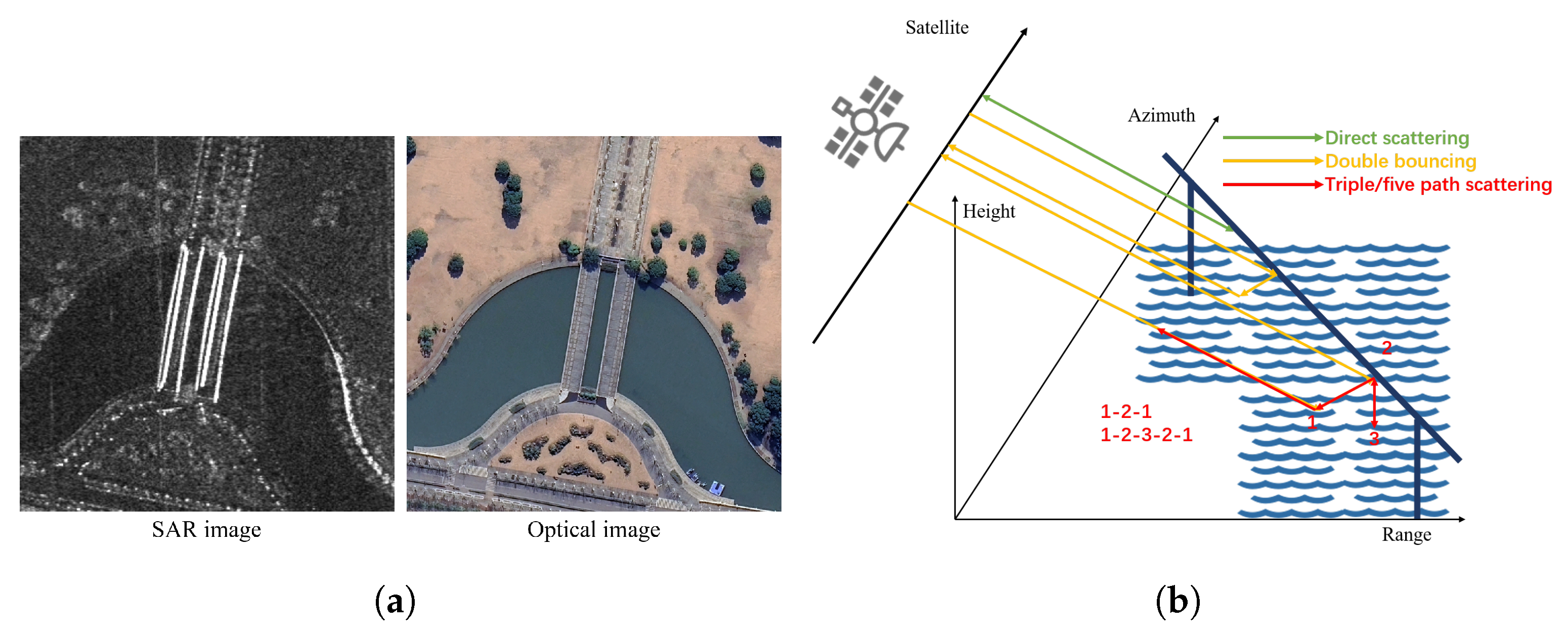
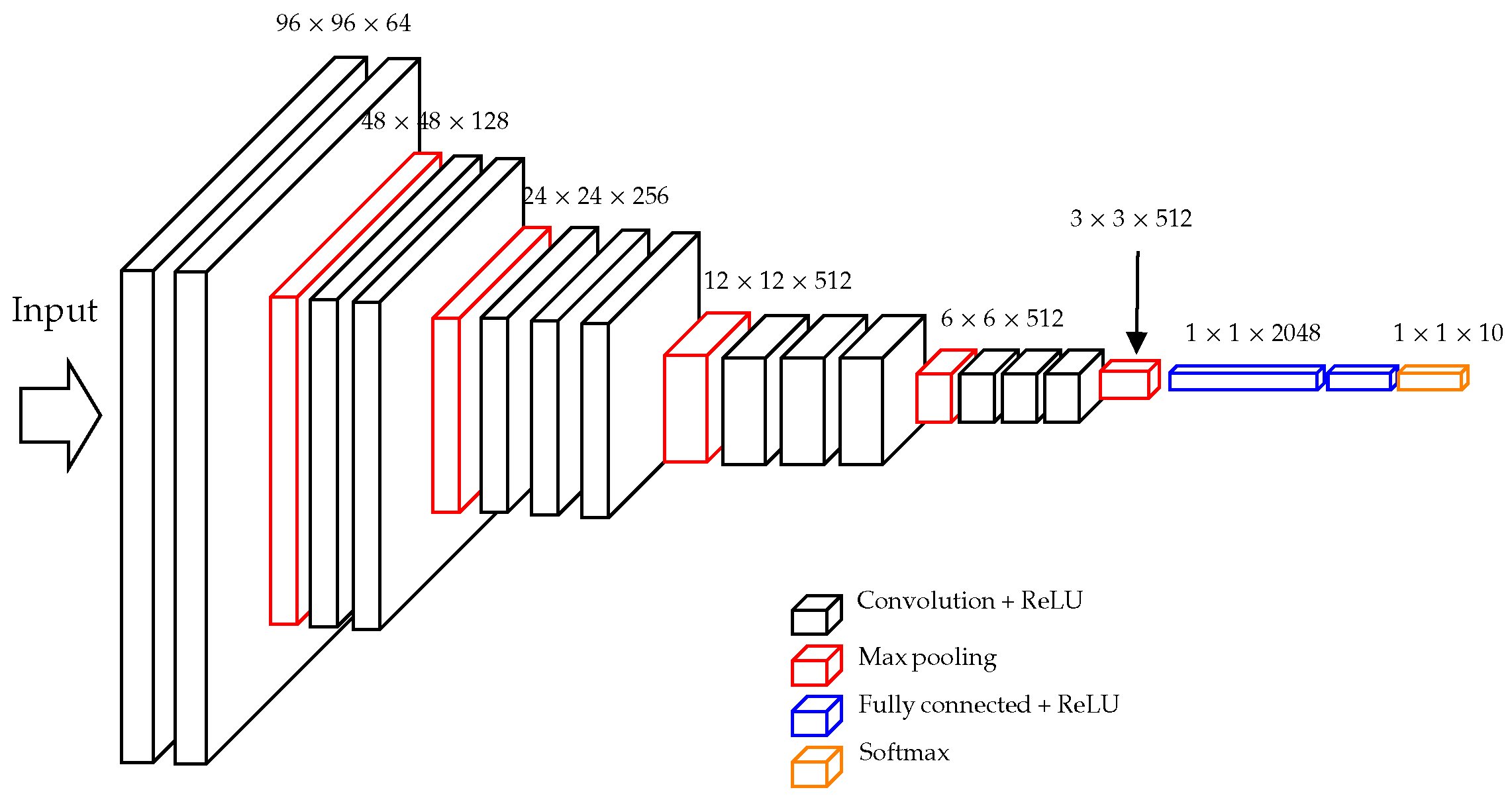
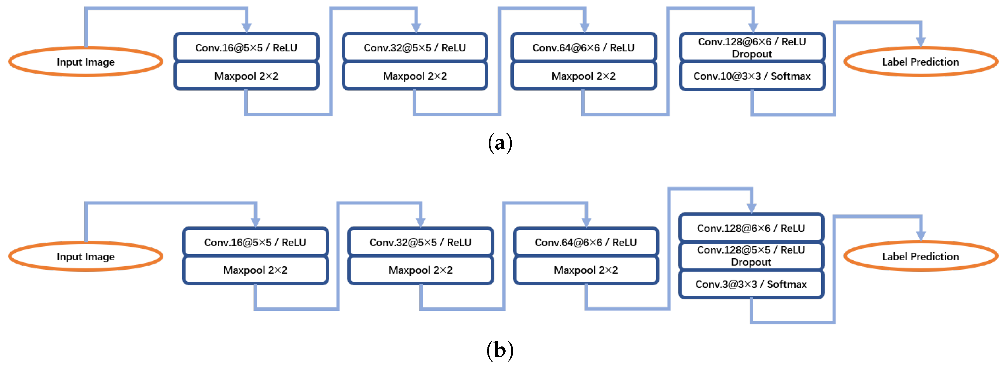
2.1. Deep Models for SAR Classification

Typical CNNs, such as VGGNet [36], ResNet [37], and DenseNet [38], have been introduced into the SAR field and achieved excellent performance [39]. In addition, some models specifically designed for SAR images have been proposed, such as A-ConvNet (ACN) [10].

The three CNNs differ significantly in terms of network capacity and architectural design. Therefore, testing and evaluating their adversarial robustness can help improve the researchers’ understanding of the different network structures and keep enhancing the robustness of the models. The CNNs used in the experiments and their structural characteristics are shown in Table 1.

Table 1. CNN architecture details and experimental adaptations for SAR image classification.

Network Family	Tested Variant	Architectural Features	Params (M) (MSTAR/OpenSARShip)	Adaptations
VGGNet [36]	VGG11 VGG16	Stacked 3 × 3 conv layers Fully connected classifiers	VGG11: 18.68/26.0 VGG16: 24.17/31.49	As shown in Figure 5, only two FC layers retained.
ResNet [37]	ResNet18 ResNet101	Residual blocks Global average pooling	ResNet18: 11.17/11.17 ResNet101: 42.5/42.5	None
AConvNet [10]	AConvNet	Large conv kernels Shallow architecture	0.39/0.79	As shown in Figure 6.

Table 1. CNN architecture details and experimental adaptations for SAR image classification.

Network Family	Tested Variant	Architectural Features	Params (M) (MSTAR/OpenSARShip)	Adaptations
VGGNet [36]	VGG11 VGG16	Stacked 3 × 3 conv layers Fully connected classifiers	VGG11: 18.68/26.0 VGG16: 24.17/31.49	As shown in Figure 5, only two FC layers retained.
ResNet [37]	ResNet18 ResNet101	Residual blocks Global average pooling	ResNet18: 11.17/11.17 ResNet101: 42.5/42.5	None
AConvNet [10]	AConvNet	Large conv kernels Shallow architecture	0.39/0.79	As shown in Figure 6.

2.2. Adversarial Attack Algorithms

Since Szegedy et al. [25] proposed the L-BFGS attack, AEs have been discovered across a wide range of domains. In the image domain, adversarial perturbations can be imperceptible to the human eye, but can easily fool the strongest DNN models. Although adversarial attacks were originally discovered in image classification tasks, they now widely exist in tasks such as semantic segmentation [40], object detection [41], and others.

The definition of AEs can vary significantly based on the specific goal. For example, in classification, the goal of AEs may be to cause misclassification (known as the untargeted attack) or to force the input image to be classified as a targeted class (known as the targeted attack [31]). Our paper focuses on demonstrating the impact of tiny adversarial perturbations on the performance of the DNN SAR classification model. Therefore, we are only interested in untargeted attack.

The threat model of AEs can be defined as follows:

$$f_{\theta }(\mathit{x}+\delta )\ne f_{\theta }\left(\mathit{x}\right)\mathrm{s}.\mathrm{t}.{\Vert \delta \Vert }_p\le ϵ.$$

(1)

As for the choice between white-box and black-box attacks, it is reasonable to assume that the attacker has full knowledge of the model structure and parameters in order to evaluate the robustness of the DNN model under the worst-case scenario. Meanwhile, white-box attack algorithms can often be extended to the case of black-box attacks, e.g., by constructing surrogate models [42] or gradient approximations [43,44]. Therefore, the selected adversarial attacks are all white-box attacks.

2.2.1. Fast Gradient Sign Attack (FGSM)

Goodfellow et al. [27] hypothesized that the decision boundary of the DNN model is locally linear and proposed the fast gradient sign method (FGSM). The FGSM generates AEs according to (2):

$$\delta =ϵ·sign\left({\nabla }_{\mathit{x}}L(F(\mathit{x};\theta ),y)\right)$$

(2)

The gradient in (2) can be calculated efficiently with back-propagation, which makes FGSM very efficient.

2.2.2. Basic Iterative Method (BIM)

The BIM [28] is an iterative adversarial attack algorithm designed based on the idea of the FGSM [27] algorithm. The BIM generates AEs using the following equation:

$${\mathit{x}}_{\mathit{i}}+\delta ={clip}_{\left(ϵ\right)}\left\{{\mathit{x}}_{\mathit{i}}+\alpha ·sign\left({\nabla }_{{\mathit{x}}_{\mathit{i}}}L(F({\mathit{x}}_{\mathit{i}};\theta ),y)\right)\right\},$$

(3)

where i denotes the iteration index, $\alpha$ is the fixed step size, and ${clip}_{\left(ϵ\right)}$ performs clipping within $ϵ$ bounds. The BIM exhibits stronger adversarial effects on highly nonlinear models.

2.2.3. Project Gradient Descent (PGD)

PGD [29] is considered one of the most aggressive attacks among all first-order attack methods. Iterative FGSM algorithms, such as the BIM [28], can be seen as ${\ell }_{\infty }$-bounded PGD algorithms. Madry et al. [29] defined adversarial training as a max-min optimization problem:

$$\underset{\theta }{min}\rho \left(\theta \right),\mathrm{s}.\mathrm{t}.\rho \left(\theta \right)={\mathbb{E}}_{(\mathit{x},y)\sim D}\left[\underset{\delta \in \mathcal{S}}{max}L(F(\mathit{x}+\delta ;\theta ),y)\right],$$

(4)

where $\mathcal{S}$ is a set of allowed perturbations and $\mathbb{E}$ is the expectation operator. The inner maximization problem represents the optimization goal of generating AEs, while the outer minimization problem is the aim of adversarial training. In practice, PGD starts with randomly perturbed images.

2.2.4. Carlini & Wagner (C&W)

The C&W algorithm generates AEs with a low ${\ell }_2$-norm and is therefore often used as a benchmark for adversarial attack algorithms [31]. Instead of optimizing the cross-entropy function, they proposed seven objective functions for optimization and selected (5) with the best performance as the objective function f by experiment:

$$f\left(\tilde{\mathit{x}}\right)=max\left(\underset{i\ne t}{max}\left\{F{(\tilde{\mathit{x}};\theta )}_i\right\}-F{(\tilde{\mathit{x}};\theta )}_t,0\right)$$

(5)

where $F{(\tilde{\mathit{x}};\theta )}_i$ is the logits output for AE $\tilde{\mathit{x}}$ corresponding to the class i and t represents the target class t [31]. They also changed variables using the tanh function, which allows the variables to be optimized over a wide range. The C&W algorithm can be expressed as (6):

$$\begin{array}{c}min\Vert {\displaystyle \frac{1}{2}}{(tanh(w)+1)-x\Vert }^2+c·f({\displaystyle \frac{1}{2}}(tanh(w)+1))\\ \mathrm{where}x+\delta ={\displaystyle \frac{1}{2}}\left(tanh\left(w\right)+1\right)\\ f(\tilde{\mathit{x}})=max(\underset{i\ne t}{max}\left\{F{(\tilde{\mathit{x}};\theta )}_i\right\}-F{(\tilde{\mathit{x}};\theta )}_t,-\kappa )\end{array}$$

(6)

where w is the object of optimization, and c is a hyperparameter to balance the ${\ell }_2$ norm and adversarial attack objective. $\kappa$ is used to control the confidence level of occurrence of misclassification. A large $\kappa$ results in a high level of confidence in the misclassification.

However, the C&W algorithm usually requires thousands of iterations to find the AE since the it performs a linear search, which is inefficient.

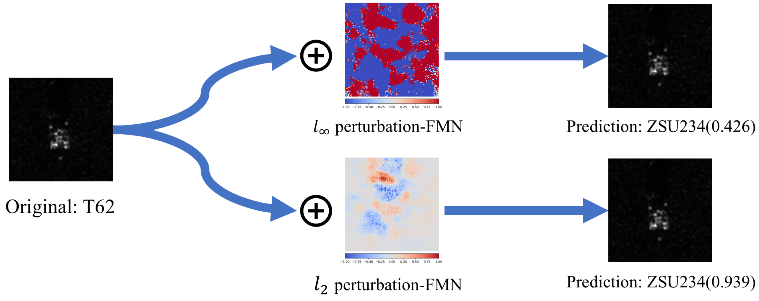
2.2.5. Fast Minimum-Norm Attack (FMN)

Pintor et al. [33] proposed the FMN attack to balance efficiency and adversarial perturbation norm searching for AEs. A constant c in (6) is difficult to choose and will cause excessive iterations in the C&W attack. So instead of constraining ${\ell }_p$-norm with a constant c, adversarial perturbation $\delta$ is projected on an $ϵ$-sphere around the original image $\mathit{x}$ for each iteration in the FMN attack [33]. The iterative process of the FMN attack is illustrated in Figure 7.

2.2.6. DeepFool

DeepFool is a simple and efficient adversarial attack algorithm based on hyperplane classification that can fool various classifiers [30]. It was originally proposed as an algorithm to evaluate the robustness of classifiers. The minimum adversarial perturbation is defined as

$$\mathsf{\Delta }(\mathit{x};f_{\theta }):=\underset{\mathit{r}}{min}{\Vert \mathit{r}\Vert }_2\mathrm{s}.\mathrm{t}.f_{\theta }(\mathit{x}+\mathit{r})\ne f_{\theta }\left(\mathit{x}\right).$$

(7)

$\mathsf{\Delta }(\mathit{x};f_{\theta })$ is called the robustness of $f_{\theta }$ at point x and DeepFool is an efficient algorithm that computes $\mathit{r}$ in (7) in order to calculate the robustness in (8). The robustness of the classifier $f_{\theta }$ on the whole test set is defined as

$${\widehat{\rho }}_{\mathrm{adv}}\left(f_{\theta }\right)={\displaystyle \frac{1}{\left|D\right|}}\sum _{\mathit{x}\in D}{\displaystyle \frac{\Vert \widehat{\mathit{r}}{\left(\mathit{x}\right)\Vert }_2}{{\Vert \mathit{x}\Vert }_2}}.$$

(8)

For a nonlinear multi-classifier with complex decision boundaries, DeepFool obtains multiple linearized boundaries for the input ${\mathit{x}}_{\mathbf{0}}$ and forms a convex polygonal region as shown in Figure 8. The AE can be crafted by simply perturbing the input ${\mathit{x}}_{\mathbf{0}}$ towards the nearest hyperplane.

3. Experiments and Results

3.1. Experimental Setup

The influence of attack and defense algorithms on DNNs is intricate due to potential interactions among datasets, training strategies, and the algorithms themselves. To isolate the effects of these algorithms, an easier dataset (MSTAR) is initially used in the experiments, allowing DNNs to achieve near-perfect precision. Following this, a more challenging dataset, OpenSARShip, is employed to further examine the impact of the attack and defense algorithms. For more complex datasets, such as large-scale, diverse-category urban classification datasets, we will offer discussions and future prospects in Section 4.2.

3.1.1. Dataset

The MSTAR dataset was collected by the Sandia National Laboratory SAR sensor platform. It contains thousands of SAR images of ground targets, including different aspect angles (in the range of 0° to 360°), different depression angles, and different types. The publicly available dataset contains 10 categories of targets (armored personnel carrier: BMP-2, BRDM-2, BTR-60, and BTR-70; main battle tanks: T-62, T-72; self-propelled howitzer: 2S1; anti-aircraft gun: ZSU-234; truck: ZIL-131; bulldozer: D7). All data were collected using an X-band SAR sensor in a 1 ft resolution spotlight mode. The MSTAR benchmark dataset is widely used in the SAR target classification field to evaluate the performance of different algorithms. The number of images of different targets in the training and testing sets is shown in

Table 2. Number of Training and testing images for the MSTAR dataset.

Class	Train Set		Test Set
	Depression	Number	Depression	Number
2S1	17°	299	15°	274
BMP2	17°	233	15°	195
BRDM2	17°	298	15°	274
BTR60	17°	256	15°	195
BTR70	17°	233	15°	196
D7	17°	299	15°	274
T62	17°	299	15°	273
T72	17°	232	15°	196
ZIL131	17°	299	15°	274
ZSU23/4	17°	299	15°	274

. Example images of 10 military targets in the MSTAR dataset are shown in Figure 9.

The OpenSARShip dataset was collected by C-band SAR of Sentinel-1 satellites. It contains 11,346 ship chips covering 17 AIS types from 41 Sentinel-1 SAR images [45]. We selected three elaborate types of ship chips for our experiments. For each chip, we select only the VH polarization. The number of images of different targets in the training and testing sets is shown in

Table 3. Distribution of training and testing images in the OpenSARShip dataset.

Class	Train Set Number	Test Set Number
Bulk	1614	403
Container	1424	355
Tanker	2130	532

. Example images of three elaborate types of ship chips in the OpenSARShip dataset are shown in Figure 10.

3.1.2. Implementation Details

We adopted the original paper structures of ResNet18 and ResNet101 [37]. For VGG11 and VGG16, due to the small dataset, we removed one fully connected layer from the original structure to relieve the overfitting problem [36].

Images in the MSTAR dataset were cropped to the size of $96\times 96$ with two channels. Images in the OpenSARShip dataset were cropped/padded to the size of $128\times 128$ with one channel. The key training parameters are set as follows: the number of training epochs is 100, the batch size is 100, the initial learning rate is 0.001, and the learning rate decreases to 0.0001 after 50 training epochs.

We set the strength of adversarial perturbations at very low levels under the constraints of the ${\ell }_2$- and ${\ell }_{\infty }$-norm to demonstrate the adversarial robustness of SAR image classification models under extreme conditions. For ${\ell }_2$ attack, eps was set to $3\times {10}^{-1}$. For ${\ell }_{\infty }$ attack, eps was set to $1/255$. For DeepFool, C&W, and FMN attacks, adversarial perturbations that exceed the ${\ell }_p$-norm constraints were projected to an $ϵ$-ball according to (9). The projection operation is simple and introduces minimal distortion to the adversarial perturbation.

$${\delta }_{\mathrm{projected}}=ϵ·{\displaystyle \frac{\delta }{{\Vert \delta \Vert }_p}}$$

(9)

Based on the perturbation strength settings and the characteristics of the adversarial attack algorithms. The six adversarial attack algorithms and their settings used in this paper are summarized in

Table 4. Parameter settings for adversarial attacks.

Attack	Type	Settings
FGSM	Gradient-based	eps = $3\times {10}^{-1}$(${\ell }_2$) $1/255$(${\ell }_{\infty }$)
BIM	Gradient-based	eps = $3\times {10}^{-1}$(${\ell }_2$) $1/255$(${\ell }_{\infty }$) iteration = 50 stride = 0.001
PGD	Gradient-based	eps = $3\times {10}^{-1}$(${\ell }_2$) $1/255$(${\ell }_{\infty }$) iteration = 50 stride = 0.001
DeepFool	Gradient-based	eps = $3\times {10}^{-1}$(${\ell }_2$) $1/255$(${\ell }_{\infty }$) iteration = 50
C&W	Optimization-based	eps = $3\times {10}^{-1}$(${\ell }_2$) iteration = 100
FMN	Optimization-based	eps = $3\times {10}^{-1}$(${\ell }_2$) $1/255$(${\ell }_{\infty }$) iteration = 20

.

In order to reduce the overhead of adversarial training, the number of iterations for PGD was set to 10, while the standard model was used as pre-trained model. The implementation of FGSM, BIM, PGD, and C&W is from CleverHans [46]. The implementation of DeepFool is from foolbox [47,48], and the implementation of FMN is based on the original paper [33].

3.2. Results and Discussion

3.2.1. Experiments on the MSTAR Dataset

The overall accuracy of the models on the MSTAR dataset after standard training and adversarial training is shown in

Table 5. Accuracy of SAR target classification model for the MSTAR dataset under ${\ell }_{\infty }$ attack (%).

	Standard Training					Adversarial Training
	ACN	VGG11	VGG16	ResNet18	ResNet101	ACN	VGG11	VGG16	ResNet18	ResNet101
Clean	98.93	98.27	99.01	99.051	97.07	98.23	97.94	99.01	99.05	96.90
FGSM	34.35	9.24	13.17	18.02	50.76	86.64	85.07	83.26	89.73	82.06
BIM	26.39	7.17	8.62	6.59	27.38	84.04	82.30	79.29	85.77	71.21
PGD	26.31	7.26	8.62	6.76	27.67	84.08	82.39	79.42	85.86	71.29
DeepFool	26.39	5.85	7.05	11.75	43.34	84.45	82.47	81.77	88.04	78.55
FMN	29.64	7.09	8.53	7.25	32.21	83.54	81.89	79.87	85.32	72.12

¹ Bold values indicate the highest accuracy in each row for the standard training models and the adversarial training models respectively. The following bold values are the same.

and

Table 6. Accuracy of SAR target classification model for the MSTAR dataset under ${\ell }_2$ attack (%).

	Standard Training					Adversarial Training
	ACN	VGG11	VGG16	ResNet18	ResNet101	ACN	VGG11	VGG16	ResNet18	ResNet101
Clean	98.93	98.27	99.01	99.05	97.07	98.23	97.94	99.01	99.05	96.90
FGSM	15.13	6.39	10.26	8.82	44.04	64.20	65.40	63.62	80.66	73.03
BIM	6.76	3.87	3.95	1.03	18.76	51.38	56.70	51.21	61.60	51.87
PGD	6.76	4.04	4.00	1.15	19.05	51.42	56.78	51.17	61.64	51.87
DeepFool	7.05	3.17	2.63	3.91	35.21	55.79	58.06	55.79	75.54	66.68
C&W	22.14	8.20	8.16	6.47	32.16	64.37	67.91	64.12	71.58	62.39
FMN	15.17	5.77	5.73	6.93	40.49	61.94	63.92	60.86	75.75	69.32

. Classification models for all five CNN backbones have near-perfect performance on CEs. However, the standard models do not seem to be resistant to adversarial attacks, even if the strength of the perturbations is extremely low. Under the measurement of ${\ell }_{\infty }$-norm, the standard models exhibit significant differences in adversarial robustness. The ResNet family and ACN are more robust to FGSM, while the VGGNet family is relatively weaker. BIM and PGD attacks are more effective for highly nonlinear decision boundaries. The ResNet family is more sensitive to BIM/PGD attacks, as the accuracy has decreased substantially compared to FGSM attacks. FMN and DeepFool are as effective as PGD in attacking ACN and VGGNet, but slightly less effective against ResNet. This reflects that under the ${\ell }_{\infty }$-norm, ResNet has a nonlinear decision boundary, making it more challenging for DeepFool and FMN to find AEs.

Under the measurement of ${\ell }_2$-norm, the comparison of robustness yields similar results: ResNet101 continues to exhibit significantly superior robustness compared to other network structures. The C&W attack uses more iterations, but it is less effective against ACN and VGGNet compared to DeepFool and FMN, while being more effective against ResNet. This indicates that C&W is still a powerful adversarial attack algorithm, though it is less efficient.

For standard models, VGGNet shows the worst robustness overall, while ACN and ResNet101 perform slightly better. VGGNet’s fully connected layers lead to more parameters and overfitting, likely contributing to its poor adversarial robustness. Despite a relatively poor generalization ability, ResNet101 is significantly more robust than other architectures, suggesting that network capacity may enhance adversarial robustness. Interestingly, ACN, with its simple structure, outperforms VGG11/VGG16/ResNet18 in robustness, indicating that model complexity does not necessarily determine adversarial robustness; smaller models might better handle overfitting, leading to stronger adversarial robustness.

As shown in Table 5 and Table 6, the accuracy of the robust models and the standard models on clean data remains essentially consistent while the robust models’ adversarial robustness is significantly improved. Since PGD is one of the strongest first-order attacks, PGD adversarial training enables the model to resist various other first-order attacks. For ${\ell }_{\infty }$-norm attacks, the robust models’ accuracy for AEs can still reach 70–90%. Additionally, the performance gap between BIM/PGD and FGSM attacks is not significant, suggesting that the nonlinearity of the robust model’s decision boundary has decreased. The robust model also shows a marked improvement in robustness against DeepFool and FMN attacks. We assume that different adversarial attack algorithms perform similarly at low perturbation intensities, allowing the robustness achieved through PGD adversarial training to generalize better across various attacks. The improvement in robustness is quite evident for VGGNet, while ResNet101 does not show a more pronounced performance. We hypothesized this is related to our adversarial training strategy: since the adversarial training is conducted by fine-tuning the standard model, the final performance is constrained by the capacity of the standard model. ResNet18 and ACN exhibit the highest robustness, achieving accuracy levels of around 85% across various attacks.

For ${\ell }_2$-norm attacks, the effectiveness of adversarial attacks shows significant differences. ResNet models are robust against FGSM attacks but are significantly impacted by BIM/PGD attacks, indicating that the decision boundary still demonstrates strong nonlinearity under the ${\ell }_2$-norm. This suggests that while ResNet can resist certain adversarial perturbations effectively, it remains vulnerable to more sophisticated attack strategies that exploit the model’s nonlinear decision boundaries. In contrast, ACN and VGGNet show less improvement in robustness, which we attribute primarily to the limitations in their architecture and capacity, leading to poorer robustness generalization.

To more broadly evaluate the robustness of the models, we tested the accuracy under different strengths of ${\ell }_{\infty }$ PGD attacks, with the results shown in Figure 11. All PGD attacks were performed with 50 iterations, and the step size was scaled proportionally with the strength. Our robust models were trained against ${\ell }_{\infty }$ PGD attack with $ϵ=1/255$, but as the strength increased, the model’s robustness rapidly degraded: when $ϵ=3/255$, the robust models’ resistance to PGD attack almost completely failed. When the strength reached 3/255 and 5/255, the effectiveness of the PGD attack on the standard models and the robust models, respectively, was saturated. Among the models, ResNet was more vulnerable to PGD attacks, with accuracy dropping more quickly as the strength increased. In contrast, ACN is less sensitive to the rise in strength, indicating that the network structure determines the inherent adversarial robustness of SAR image classification models.

The t-SNE visualization results of the ResNet18 models’ outputs under different adversarial attacks on the MSTAR dataset are presented in Figure 12. For CEs, the visualization results of both the standard and robust models demonstrate 10 clearly separated clusters. However, the standard models show almost no generalization ability on AEs, as the clear 10 clusters can no longer be seen in the visualization results of Figure 12. The outputs of most of the AEs have been completely mixed up. The robust models, on the other hand, still maintain a relatively good classification ability, and it is easy to see from Figure 12 that although the adversarial attack has caused many points to be shifted, the clusters of the different categories have not been completely mixed up with each other. This indicates that the AEs have not yet crossed the decision boundary of the robust models, thus still retain a certain degree of adversarial robustness.

With the help of the t-SNE visualization, we can also see the category preferences of the AEs. When comparing the results of the robust model before and after the FGSM attack in Figure 12, it is easy to observe that 2S1 (blue point) is more likely to be shifted toward BTR70 (purple point) and T62 (pink point) when attacked by FGSM, while T62 is more likely to be shifted toward ZSU23/4 (cyan point). When comparing the BIM and PGD attack in Figure 12, it is clear that the robust model is still capable of accurately classifying D7 (brown point) after the PGD attack, whereas the standard model is highly prone to confusing D7 with ZSU23/4 (cyan point).

Figure 13 shows the histogram comparison of FMN adversarial perturbation norms between standard and robust models on the MSTAR test set. The original perturbation data was used (i.e., without applying projection to constrain the norm), which explains why the ${\ell }_p$ norm shown on the x-axis exceeds the limits. The histograms show that PGD adversarial training generally increases FMN perturbation norm, reducing attack success rate. However, the variation in perturbation norms differs significantly across different backbones and norm types, and is uneven across AEs, with some showing reduced perturbation norms.

For the ${\ell }_{\infty }$ norm, ResNet101 and ACN standard models display greater robustness in Table 5, with larger FMN norm distributions in Figure 13. In contrast, the robust ResNet101 model shows weaker robustness, as most AEs exhibit smaller FMN norms despite a few having very large values.

For the ${\ell }_2$ norm, the ResNet101 standard model shows stronger robustness, though the perturbation norm is relatively smaller compared to other backbones. Adversarial training effects vary: VGG16 and ResNet101 show modest improvements, while ACN, VGG11, and ResNet18 experience greater gains. However, the FMN perturbation norm does not always correlate with accuracy. The robust ResNet18 model has a smaller FMN perturbation norm but higher accuracy than ACN and VGGNet, and while the robust ResNet101 model has smaller norms, it still outperforms others in some cases.

3.2.2. Experiments on the OpenSARShip Dataset

The overall accuracy of the SAR image classification models on the OpenSARShip dataset is shown in

Table 7. Accuracy of SAR target classification model for the OpenSARShip dataset under ${\ell }_{\infty }$ attack (%).

	Standard Training					Adversarial Training
	ACN	VGG11	VGG16	ResNet18	ResNet101	ACN	VGG11	VGG16	ResNet18	ResNet101
Clean	83.25	79.61	79.22	81.00	82.32	83.10	79.38	78.99	82.79	82.79
FGSM	56.58	41.00	31.00	27.59	24.26	78.45	71.93	72.40	74.72	76.12
BIM	52.71	31.08	22.32	12.09	11.24	77.67	70.23	70.23	71.86	75.27
PGD	52.86	31.00	22.40	12.09	11.24	77.67	70.23	70.23	71.86	75.27
DeepFool	46.04	26.58	17.05	15.50	11.62	71.93	63.79	63.79	67.28	71.08
FMN	44.96	22.17	13.87	1.16	6.74	71.63	62.71	61.78	64.88	71.08

and

Table 8. Accuracy of SAR target classification model for the OpenSARShip dataset under ${\ell }_2$ attack (%).

	Standard Training					Adversarial Training
	ACN	VGG11	VGG16	ResNet18	ResNet101	ACN	VGG11	VGG16	ResNet18	ResNet101
Clean	83.25	79.61	79.22	81.00	82.32	83.10	79.38	78.99	82.79	82.79
FGSM	47.98	33.41	28.99	31.78	38.76	66.04	61.16	62.09	64.03	64.96
BIM	38.60	20.62	17.20	12.24	11.70	61.86	54.41	58.60	51.24	47.36
PGD	38.68	20.62	17.28	12.24	11.78	61.86	54.41	58.52	51.47	47.36
DeepFool	34.41	15.96	10.23	16.35	21.47	55.50	48.68	49.76	51.93	55.96
C&W	46.66	32.55	29.22	18.68	19.38	63.79	56.43	60.31	55.58	56.66
FMN	36.82	17.59	13.02	14.34	17.21	56.43	50.00	50.93	53.48	54.96

. The OpenSARShip dataset is more challenging due to the large range of variation in target size and complex sea surface conditions. The classification accuracy of five different backbones is around 80%, with the largest and smallest backbones (ACN and ResNet101) achieving better results. Similar to the results on the MSTAR dataset, standard models are highly susceptible to AEs. However, ACN consistently dominates in terms of robustness under both norm constraints, while the ResNet standard models show weaker robustness, especially when subjected to the BIM/PGD.

After adversarial training, the accuracy of robust ACN and VGGNet models on clean data slightly decreased. Interestingly, the accuracy of the robust ResNet models increased compared to standard models. This suggests that, with limited training data, SAR image classification models are prone to converge to locally optimal points that exhibit poor robustness. AEs can serve as a form of data augmentation, helping to regularize and mitigate overfitting, thereby improving model performance.

Under the ${\ell }_{\infty }$-norm, the robust models of ACN and ResNet demonstrate significantly stronger robustness against various adversarial attacks compared to VGGNet. Under the ${\ell }_2$-norm, the robust ACN model continues to dominate. While the robust ResNet models show good robustness against FGSM, DeepFool, C&W, and FMN, they are very vulnerable to BIM and PGD.

We also tested the accuracy under different strengths of ${\ell }_{\infty }$ PGD attacks for the OpenSARShip dataset, with the results shown in Figure 14. As the attack strength increases, the PGD on both the standard and robust models quickly reaches saturation. The differences in robustness across different network architectures become more pronounced: in the standard models, AConvNet’s accuracy drops to its lowest when $ϵ=5/255$, VGGNet reaches its lowest accuracy when $ϵ=3/255$, while ResNet drops to its lowest when $ϵ=1/255$. This further highlights the impact of network architecture on model robustness.

The t-SNE visualization results of the ACN outputs under different attacks on the OpenSARShip dataset are presented in Figure 15. Unlike the results on the MSTAR dataset, the classification visualization results on OpenSARShip show less clear boundaries between clusters. Considering the targets in OpenSARShip are more complex in terms of size, angle, and scattering characteristics, classification models find it difficult to distinguish many targets, resulting in numerous points lying close to the decision boundaries. From Figure 15, it can be observed that after being attacked, the classification models are prone to confuse Bulk (blue point) and Container (orange point), while the Tanker (green point) category is relatively less affected. Since both container and bulk fall under the cargo ship category, they share many similarities in shape and structure, making them more challenging for the model to differentiate [45]. Since the attack intensity of FGSM/BIM/PGD attacks on images is determined by parameters, it can be seen from Figure 15 that the visualization results present extremely chaotic points. In contrast, DeepFool and FMN dynamically adjusted attack intensity. Therefore, in the visualization results, it can be seen that the outputs of the AEs are concentrated near the decision boundary of the model, which are represented as curved boundaries in the figures.

Similar to the MSTAR dataset, Figure 16 compares FMN adversarial perturbation norms between standard and robust models on the OpenSARShip test set.

For the ${\ell }_{\infty }$ norm, the ACN standard model shows stronger robustness, as indicated by the relatively larger perturbation norms in the histogram. In contrast, VGGNet and ResNet standard models have many perturbation norms clustered near zero, likely contributing to weaker robustness. For robust models, all backbones show improvements, with ResNet101 having the largest perturbation norms, though its accuracy remains lower than ACN’s.

For the ${\ell }_2$ norm, the ACN standard model has larger perturbation norms, consistent with its accuracy. Despite smaller perturbation norms, the ResNet models outperform VGG16 under FGSM, DeepFool, and FMN attacks in accuracy. After adversarial training, perturbation norms for ACN, VGG16, and ResNet models increased. Interestingly, the VGG11 robust model showed minimal change in the distribution of perturbation norms, with some AEs even decreasing, yet its accuracy improved significantly.

From Figure 13 and Figure 16, we conclude as follows:

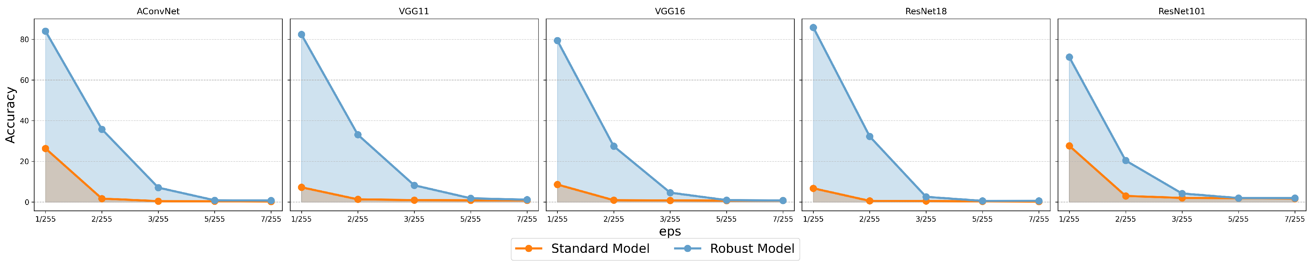
• Model-Specific Perturbation Norms: Adversarial perturbation magnitudes vary by architecture and are incomparable across models.
• Complex Decision Boundary: FMN’s $ϵ$-ball projection enables successful large-norm attacks, revealing mismatches between perturbation magnitude and robustness.
• Unstable Defense Gains: PGD adversarial training inconsistently increases perturbation norms across models and images, limiting reliability.

Further exploration is needed for accurate and fair assessment of adversarial robustness in SAR image classification models.

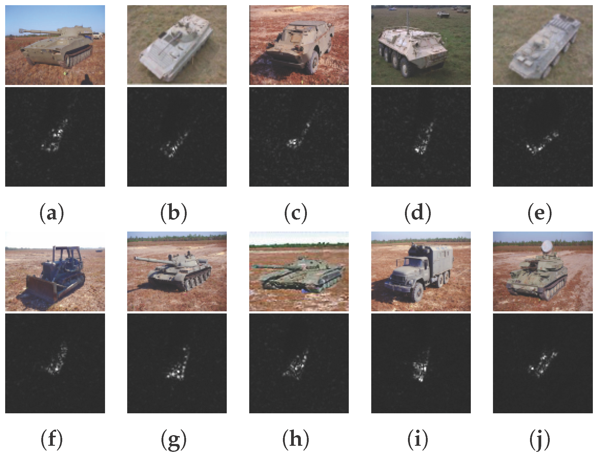
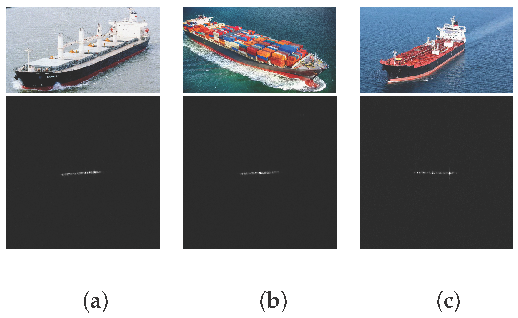
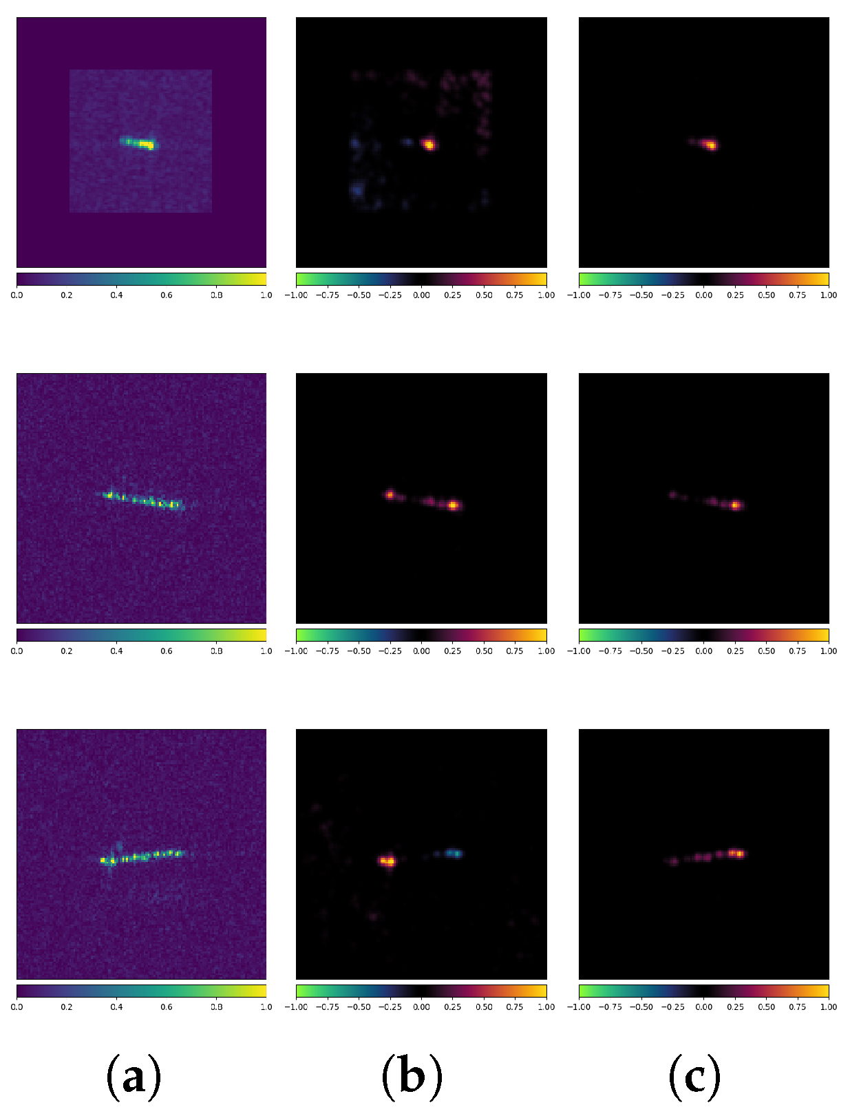
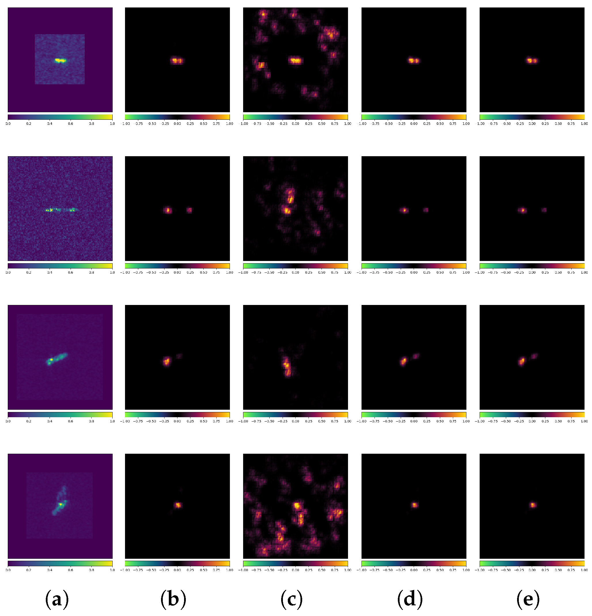
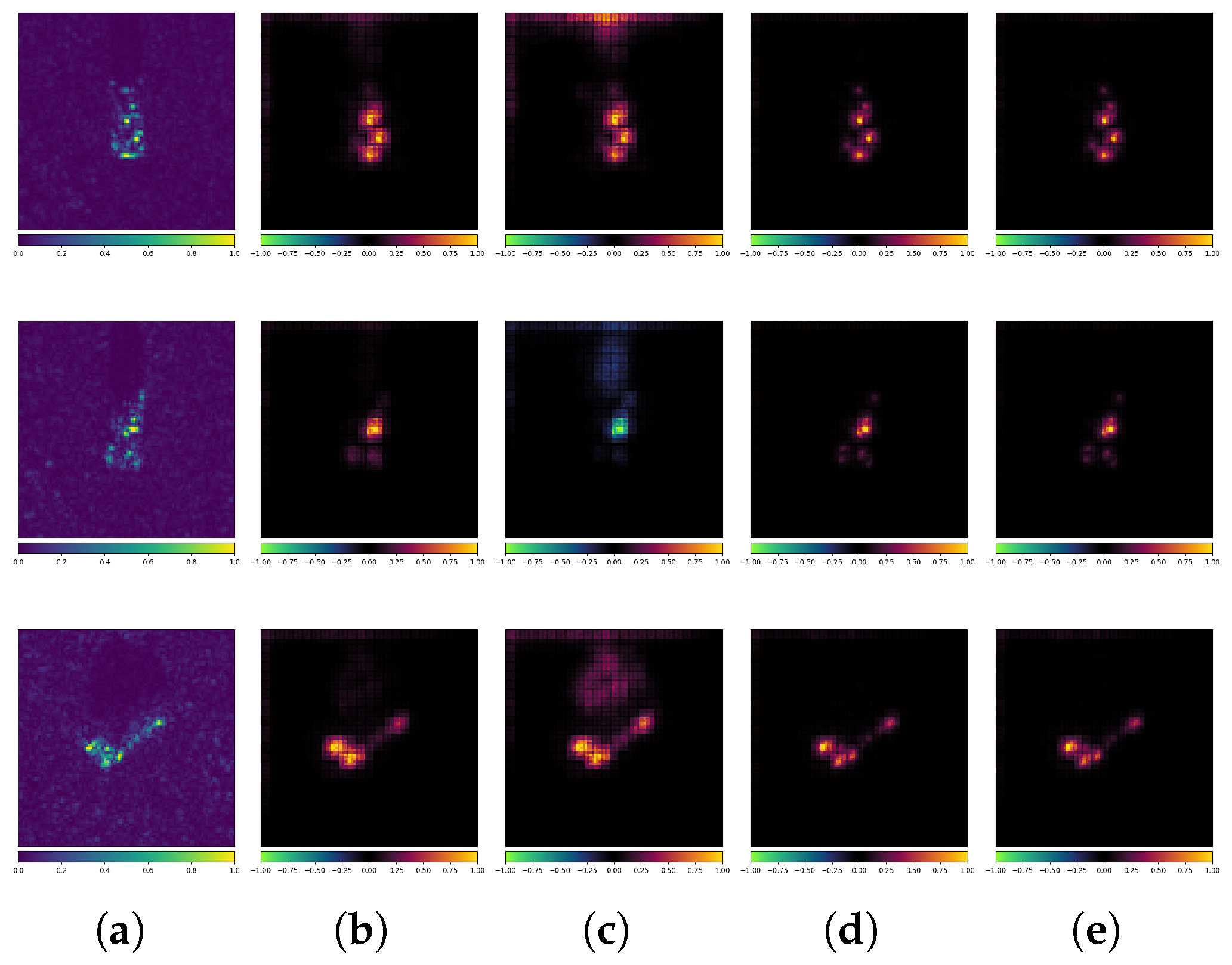
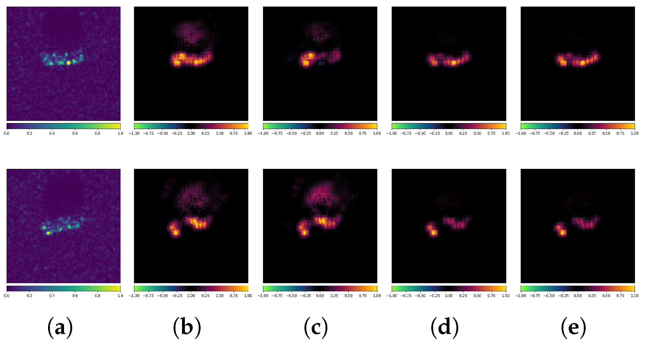
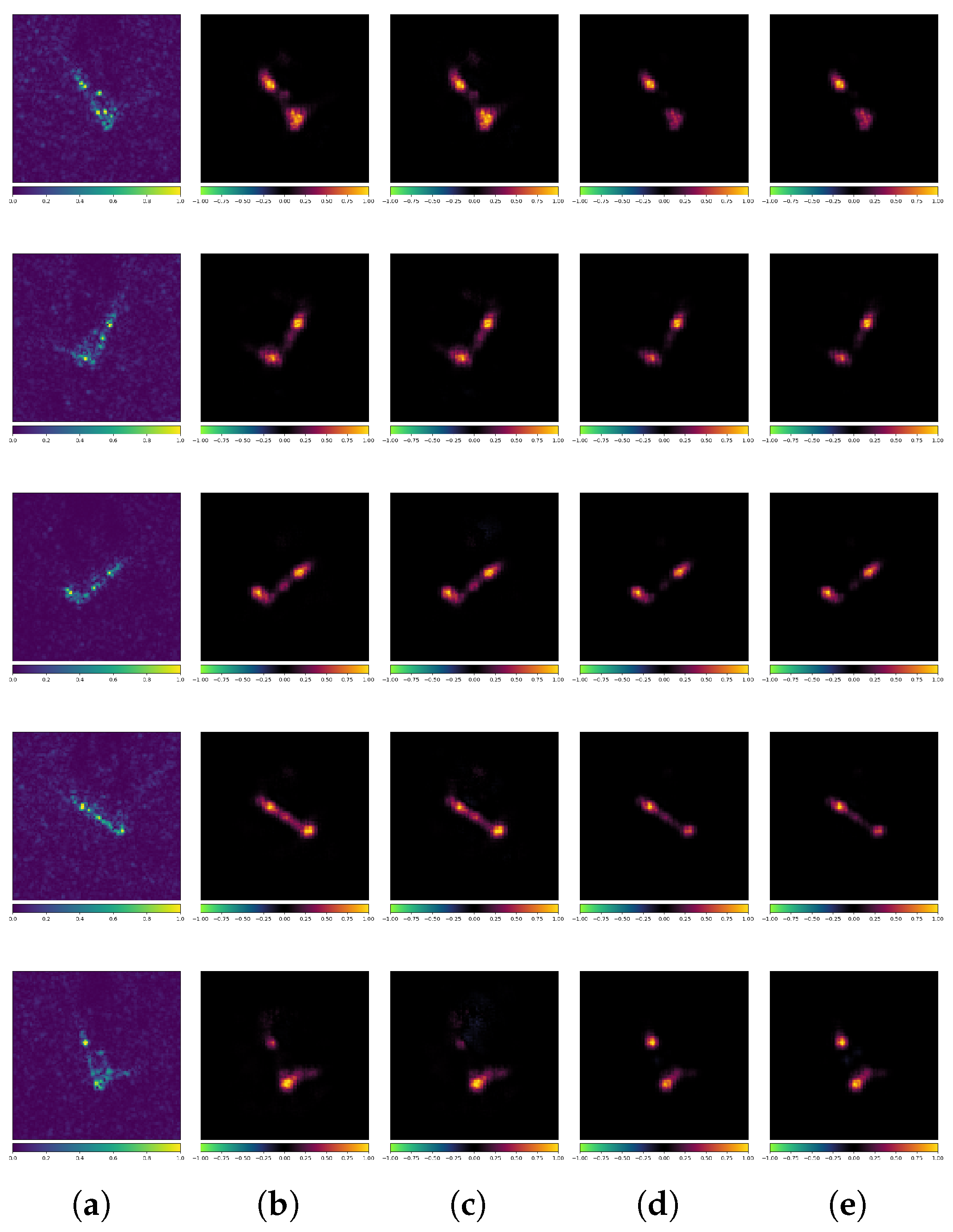
3.3. Interpretability Analysis

The experimental results on both datasets indicate that the standard models perform well on CEs but are highly vulnerable to AEs. For the robust models, though their accuracy on CEs may be hurt due to adversarial training, they have much stronger adversarial robustness. This suggests a change in the models’ decision-making, resulting in a significant improvement in adversarial robustness.

To explain the diverse DNN models, researchers have proposed various XAI methods, such as Grad-CAM [49], which is widely applied in CNNs; LIME [50] based on perturbation and linear approximation; and SHAP [51] based on Shapley values. XAI methods offer the opportunity to open the “black box” of DNNs, providing a more intuitive understanding of the relationship between model behavior and adversarial robustness. However, the attribution effects of different XAI methods may vary significantly:

• Grad-CAM: High computational efficiency but low resolution, making it challenging to capture detailed structures in SAR images.
• LIME: Not limited by model structure, but results are influenced by perturbations, leading to instability.
• SHAP: High computational complexity, making it unsuitable for large datasets with high resolution.
• LRP: High-precision attribution, moderate computational complexity, closely related to the network architecture.

Consequently, we chose the LRP [52], which offers a balance between computational complexity and attribution precision.

Figure 17 presents an example where both the standard and robust models correctly classify the CEs. The true label for all three images is Bulk. It is evident that despite the consistent classification results, the attribution maps exhibit significant differences (note that both models use the VGG16 architecture). The standard model’s classification is more influenced by the background regions, whereas the robust model focuses more on the target itself. Additionally, their methods of selecting feature scattering characteristics from the same target differ noticeably, sometimes even highlighting completely opposite features. For example, in the third row, the standard model’s prediction is primarily influenced by scattering characteristics at both ends of the target (where the blue region in the attribution map indicates a negative correlation with the model’s prediction). In contrast, the robust model’s prediction is mainly influenced by the scattering characteristics on the right and center of the target (where the red region in the attribution map indicates a positive correlation with the model’s prediction).

Figure 18 shows ResNet101 attribution maps for clean examples (CEs) and PGD adversarial examples (AEs) labeled “Container”. The standard model correctly classifies CEs but misclassifies AEs, focusing on irrelevant background features instead of targets. Conversely, the robust model classifies both correctly and maintains consistent attribution maps across CEs and AEs.

Figure 19 and Figure 20 show additional MSTAR examples (true labels: 2S1 and BTR60). Both models correctly classify CEs, but only the robust model correctly classifies AEs. Attribution maps confirm that strong scattering characteristics remain critical for SAR image interpretation. While standard models fail to capture these features and overfit to background/shadow interference, robust models effectively learn scattering characteristics and mitigate overfitting, particularly against AEs, demonstrating that adversarial training can indeed mitigate overfitting problems.

Figure 21 presents a set of examples of DeepFool AEs. The true label is ZIL213. The standard model misclassified the AEs as 2S1, while the robust model classified them correctly. Since DeepFool aims to find the minimal ${\ell }_p$-norm perturbation that causes the AE to cross the model’s decision boundary, the perturbations are further reduced. Therefore, even if the model’s predictions were incorrect, the differences are rather small. However, we can still observe significant differences between the standard model and the robust model from the attribution maps in Figure 21. For example, in the first row, the robust model is less influenced by the scattering characteristics at the bottom of the target. In the third and fourth rows, the robust model clearly reduces its attention to the scattering characteristics in the middle of the target. In the fifth row, the robust model strengthens its attention to the scattering characteristics at the top of the target. From the perspective of extracting semantic features, while PGD and DeepFool differ fundamentally in their attack mechanisms, the robust model can defend against DeepFool by extracting more interpretable and resilient scatterer features from SAR images.

The examples above demonstrates that adversarial training demonstrably mitigates overfitting while substantially enhancing feature extraction efficacy. However, both standard and robust models exhibit a perplexing phenomenon: they primarily leverage only a limited subset of target scatterer characteristics in SAR images. Sometimes, SAR image classification models tend to focus on limited local information when making predictions, while paying insufficient attention to the global scattering structure. This decision pattern may indicate potential issues with the interpretability of such models, as it diverges from the conventional understanding in SAR-ATR, where comprehensive scattering structure analysis is conventionally deemed essential.

From the comparison of the attribution maps above, we can conclude the following:

• Enhanced Learning of Strong Scattering Characteristics: In SAR image classification, PGD adversarial training helps the model to better learn the strong scattering characteristics within SAR images.
• Mitigation of Overfitting: PGD adversarial training helps mitigate overfitting, enabling the model to learn real features rather than spurious ones.
• Anomalies in Misclassified AEs: When misclassification occurs, the attribution maps for AEs often show significant anomalies, which may be related to the model’s adversarial vulnerability.
• Selective Scattering Attention in Attribution Maps: SAR image classification models exhibit selective focus on scattering characteristics. This explainability gap suggests adversarial robustness mechanisms may diverge from human-physics expectations.

It is important to note that not all misclassified AEs will show significant differences in LRP attribution maps, which may be related to the limitations of XAI method. The role of the XAI method in analyzing AEs and adversarial robustness requires further investigation.

4. Discussion and Prospects for Intricate Urban Classification Datasets

4.1. Discussions

Based on the experimental results from MSTAR and OpenSARShip, we can draw some preliminary conclusions and speculations regarding the adversarial robustness of SAR classification models, summarized as follows:

• Large networks are not as robust as expected in SAR image classification. Pre-trained models or more effective data augmentation methods are necessary.
  Due to the generally small size of SAR image datasets, the training strategy has a significant impact on model performance and robustness. Larger networks within the same family, such as VGGNet and ResNet, often perform worse than smaller ones. At the same time, large networks, such as VGG16 and ResNet101, often perform worse than smaller networks like AConvNet. AEs, an effective data augmentation technique, help mitigate overfitting and enhance the robustness of larger models, warranting further study and application in SAR image classification.
• Low-intensity adversarial training achieves contextual robustness for SAR image classification but has intrinsic limitations.
  Our controlled experiments identify that low-intensity PGD adversarial training (eps = 1/255) enhance model robustness with minimal accuracy loss (<1% on both datasets). This aligns with adversarial training’s dual role as regularizer and implicit data augmenter [27]. However, three fundamental limitations persist:
  • Attack-type overfitting: Defense efficacy collapses under unseen threat models.
  • Intensity brittleness: Robustness plummets beyond trained eps thresholds.
  • Semantic blindness: Digital adversarial perturbations lack semantic and physical information.
  We thus advocate a multi-layered defense strategy combining adversarial detection (artifact screening) and feature disentanglement (scattering physics preservation) for operational SAR image classification systems.
• DNN architecture determines the adversarial robustness of the SAR image classification model.
  While clean-data accuracy was comparable across networks, robustness varied substantially: Linear layers (e.g., in VGGNet) increased overfitting without improving robustness. Residual connections (e.g., in ResNet) enhanced adversarial trainability despite initial BIM/PGD vulnerability. Large convolutional kernels (e.g., in ACN) optimally captured scattering features with inherent robustness.
  The recommended design principles are abort linear layers and apply large convolutional kernels and adversarial-trained residual blocks for SAR image classifiers.
• XAI reveals the underlying mechanisms of adversarial robustness in SAR through saliency physics.
  Beyond conventional metrics, attribution maps generated by LRP expose sample-specific decision logic:
  • Adversarial training induces saliency shift from background artifacts to target scattering signatures.
  • Robust models develop scattering-point coherence—preserving key bright spots under perturbation.
  This human-aligned interpretability bridges geometric scattering principles with DNN’s hierarchical feature learning, enabling causal analysis of adversarial vulnerabilities.

White-box and black-box adversarial attacks, while distinct in their methodologies, share underlying principles that can bridge the gap between them. As shown in Figure 22, white-box attacks involve crafting AEs with full knowledge of the target model’s architecture and parameters, allowing for finer perturbations. In contrast, black-box attacks operate under the assumption that the attacker has no access to the model’s internal details, relying instead on outputs such as class labels or probabilities.

To better align adversarial attacks with black-box scenarios, researchers have developed numerous effective black-box strategies. The HopSkipJump attack (HSJA) is a powerful black-box attack that only requires final class prediction [43]. HSJA attack generates the AEs in each iteration by binary search, gradient direction estimation, and step size computation. Wu et al. [42] proposed the attention-guided transfer attack (ATA) algorithm by combining attention and transferability of AEs. Experiments prove that ATA is far more lethal than white-box attacks such as the FGSM and BIM.

Numerous studies have also shown that, despite the differences between white-box and black-box scenarios, the transferability of AEs can effectively enable the application of white-box attack methods in black-box settings. This transferability means that AEs generated through white-box methods can often deceive black-box models, especially when there is structural similarity between the models. For instance, research has demonstrated that AEs crafted for one model can effectively attack another model without direct access to its internal parameters [43]. Zhang et al. [53] conducted a comprehensive study on the impact of data augmentation and gradient regularization on the transferability of surrogate models under black-box attacks. Notably, their experiments still relied on the PGD for generating AEs. Compared to white-box settings, black-box attacks involve more complex scenarios and are influenced by a broader range of factors, making them more difficult to compare and evaluate. However, existing research has shown that many conclusions drawn from white-box attacks still hold in black-box settings.

In practical applications, particularly in the physical domain, the distinction between white-box and black-box attacks becomes less pronounced. Physical adversarial attacks often exploit the inherent transferability of AEs, allowing techniques developed in white-box settings to be effective in black-box contexts [54]. Studies have shown that AEs generated in controlled environments can successfully deceive target models in real-world scenarios, underscoring the importance of considering both attack types in comprehensive security assessments [55].

Given the prevalence of black-box attacks in practical scenarios, it is essential to explore and understand their dynamics. Future research will focus on developing and evaluating adversarial attack methods specifically designed for black-box settings, particularly in the physical domain, to enhance the robustness and security of machine learning models against a broader range of adversarial threats.

4.2. Prospects for LULC

While our current study focuses on single-target SAR-ATR scenarios, the fundamental scattering mechanisms governing SAR imaging remain physically consistent across different scales. In LULC tasks, large-scale urban SAR images exhibit more complex scattering center distributions. For example, the OpenSARUrban dataset [56] focuses on interpreting urban SAR images and encompasses 10 distinct categories. Some categories, such as general residential areas, storage areas, and high-rise buildings, exhibit very similar features, posing significant challenges for accurate classification. Another instance is the complex-valued SAR classification dataset in [57], which includes diverse urban areas and presents even greater classification difficulties. Aside from the difference in scale, their elementary scattering components—such as dihedral structures from building walls, trihedral reflections from roof–ground interactions, and Bragg scattering from vegetation—are essentially the same. The cross-scale physical homogeneity motivated our choice of single-target analysis: by decoupling target–background interference, it is possible to align the LRP method with the physical characteristics of SAR images.

Crucially, our adversarial robustness studies reveal transferable insights: robust models exhibit a systematic attention shift from localized high-intensity scatterers to distributed structural correlations. This behavioral transition aligns with the physical principle that robust SAR recognition should depend on geometric configuration invariances rather than transient bright points. Given that urban LULC taxonomies are ultimately defined by spatial arrangements of these canonical scattering elements, we propose three transfer pathways for complex scene classification:

• Hierarchical attention mechanisms bridging atomic (single-target) and molecular (scene-level) scattering patterns.
• Invariant feature learning capturing scale-independent scattering topologies through equivariant networks.
• Curriculum Adversarial Training (CAT) [58] progressively increasing scene complexity from isolated targets to cluttered urban mosaics.

To validate this framework, future work will extend our adversarial evaluation methodology. It is essential to utilize multiple types of AEs to thoroughly assess the adversarial robustness of DNN models for such intricate classification tasks. Moreover, incorporating multiple adversarial defense methods, such as AE detection [59] and model distillation [60], is crucial, considering the prevalence of AEs in high-dimensional spaces where simple adversarial training may not suffice. Furthermore, the development of more efficient methods to evaluate the adversarial robustness of DNN models is beneficial for monitoring model accuracy during training. Nonetheless, we can still anticipate the following prospects for SAR classification models:

• The DNN structure should be adapted to the characteristics of the dataset. Larger models do not necessarily have better performance or adversarial robustness.
• Reduce unnecessary weight parameters in DNNs. Using adaptive pooling or convolutional layer instead of fully connected layers may result in better adversarial robustness.
• In SAR image classification, AEs should be used as an effective means of regularization and overfitting mitigation, which may potentially improve model performance in certain cases.
• Adversarial training using pre-trained models can accelerate convergence, making the model’s accuracy more controllable.

To facilitate further research, all types of data from this experiment can be obtained from https://opensar.sjtu.edu.cn/ (accessed on 16 May 2025).

5. Conclusions

The performance of deep SAR image classification models far exceeds that of traditional methods, but the interpretability and robustness of the deep SAR image classification models are still highly problematic. Since SAR image datasets are usually limited in size, a suitable CNN backbone needs to be selected for the dataset. Large networks with more parameters may perform poorly due to overfitting problems and also have fragile adversarial robustness.

Adversarial training is an effective way to improve the adversarial robustness of the deep SAR image classification models, but it suffers from the problem of algorithmic limitations. It is certainly frustrating if we spend a lot of time and computing power to obtain a robust model that can only withstand a specific class of adversarial attack algorithms. The XAI method provides powerful tools for understanding and improving adversarial robustness. Effective utilization of attribution results and further improvement of XAI remain interesting research directions.

To improve the adversarial robustness of DNN models, the key lies in improving the neural network structure and training methods.

References

1. Guo, W.; Zhang, Z.; Yu, W.; Sun, X. Perspective on explainable SAR target recognition. J. Radars 2020, 9, 462–476. [Google Scholar] [CrossRef]
2. Huang, Z.; Yao, X.; Liu, Y.; Dumitru, C.O.; Datcu, M.; Han, J. Physically explainable CNN for SAR image classification. ISPRS J. Photogramm. Remote Sens. 2022, 190, 25–37. [Google Scholar] [CrossRef]
3. Huang, Z.; Wu, C.; Yao, X.; Zhao, Z.; Huang, X.; Han, J. Physics inspired hybrid attention for SAR target recognition. ISPRS J. Photogramm. Remote Sens. 2024, 207, 164–174. [Google Scholar] [CrossRef]
4. Huang, Z.; Datcu, M.; Pan, Z.; Lei, B. Deep SAR-Net: Learning objects from signals. ISPRS J. Photogramm. Remote Sens. 2020, 161, 179–193. [Google Scholar] [CrossRef]
5. Zhu, Y.; Ai, J.; Wu, L.; Guo, D.; Jia, W.; Hong, R. An Active Multi-Target Domain Adaptation Strategy: Progressive Class Prototype Rectification. IEEE Trans. Multimed. 2025, 27, 1874–1886. [Google Scholar] [CrossRef]
6. Tian, Z.; Wang, W.; Zhou, K.; Song, X.; Shen, Y.; Liu, S. Weighted Pseudo-Labels and Bounding Boxes for Semisupervised SAR Target Detection. IEEE J. Sel. Top. Appl. Earth Obs. Remote Sens. 2024, 17, 5193–5203. [Google Scholar] [CrossRef]
7. Deng, J.; Wang, W.; Zhang, H.; Zhang, T.; Zhang, J. PolSAR Ship Detection Based on Superpixel-Level Contrast Enhancement. IEEE Geosci. Remote Sens. Lett. 2024, 21, 1–5. [Google Scholar] [CrossRef]
8. Chen, S.; Wang, H. SAR target recognition based on deep learning. In Proceedings of the 2014 International Conference on Data Science and Advanced Analytics (DSAA), Shanghai, China, 30 October–1 November 2014; IEEE: Piscataway, NJ, USA, 2014; pp. 541–547. [Google Scholar]
9. Morgan, D.A.E. Deep convolutional neural networks for ATR from SAR imagery. In Algorithms for Synthetic Aperture Radar Imagery XXII; Zelnio, E., Garber, F.D., Eds.; International Society for Optics and Photonics, SPIE: Bellingham, WA, USA, 2015; Volume 9475, p. 94750F. [Google Scholar] [CrossRef]
10. Chen, S.; Wang, H.; Xu, F.; Jin, Y.Q. Target Classification Using the Deep Convolutional Networks for SAR Images. IEEE Trans. Geosci. Remote Sens. 2016, 54, 4806–4817. [Google Scholar] [CrossRef]
11. Lin, Z.; Ji, K.; Kang, M.; Leng, X.; Zou, H. Deep Convolutional Highway Unit Network for SAR Target Classification With Limited Labeled Training Data. IEEE Geosci. Remote Sens. Lett. 2017, 14, 1091–1095. [Google Scholar] [CrossRef]
12. Zhao, P.; Liu, K.; Zou, H.; Zhen, X. Multi-stream convolutional neural network for SAR automatic target recognition. Remote Sens. 2018, 10, 1473. [Google Scholar] [CrossRef]
13. Huang, G.; Liu, X.; Hui, J.; Wang, Z.; Zhang, Z. A novel group squeeze excitation sparsely connected convolutional networks for SAR target classification. Int. J. Remote Sens. 2019, 40, 4346–4360. [Google Scholar] [CrossRef]
14. Wang, W.; Zhang, C.; Tian, J.; Ou, J.; Li, J. A SAR Image Target Recognition Approach via Novel SSF-Net Models. Comput. Intell. Neurosci. 2020, 2020, 1–9. [Google Scholar] [CrossRef] [PubMed]
15. Wang, B.; Jiang, Q.; Song, D.; Zhang, Q.; Sun, M.; Fu, X.; Wang, J. SAR vehicle recognition via scale-coupled Incep_Dense Network (IDNet). Int. J. Remote Sens. 2021, 42, 9109–9134. [Google Scholar] [CrossRef]
16. Feng, S.; Ji, K.; Wang, F.; Zhang, L.; Ma, X.; Kuang, G. PAN: Part Attention Network Integrating Electromagnetic Characteristics for Interpretable SAR Vehicle Target Recognition. IEEE Trans. Geosci. Remote Sens. 2023, 61, 1–17. [Google Scholar] [CrossRef]
17. Zhou, Y.; Wang, H.; Xu, F.; Jin, Y.Q. Polarimetric SAR Image Classification Using Deep Convolutional Neural Networks. IEEE Geosci. Remote Sens. Lett. 2016, 13, 1935–1939. [Google Scholar] [CrossRef]
18. Zhang, Z.; Wang, H.; Xu, F.; Jin, Y.Q. Complex-Valued Convolutional Neural Network and Its Application in Polarimetric SAR Image Classification. IEEE Trans. Geosci. Remote Sens. 2017, 55, 7177–7188. [Google Scholar] [CrossRef]
19. Chen, S.W.; Tao, C.S. PolSAR image classification using polarimetric-feature-driven deep convolutional neural network. IEEE Geosci. Remote Sens. Lett. 2018, 15, 627–631. [Google Scholar] [CrossRef]
20. Liu, X.; Jiao, L.; Tang, X.; Sun, Q.; Zhang, D. Polarimetric Convolutional Network for PolSAR Image Classification. IEEE Trans. Geosci. Remote Sens. 2019, 57, 3040–3054. [Google Scholar] [CrossRef]
21. Dong, H.; Zou, B.; Zhang, L.; Zhang, S. Automatic Design of CNNs via Differentiable Neural Architecture Search for PolSAR Image Classification. IEEE Trans. Geosci. Remote Sens. 2020, 58, 6362–6375. [Google Scholar] [CrossRef]
22. Cao, Y.; Wu, Y.; Li, M.; Liang, W.; Hu, X. DFAF-Net: A Dual-Frequency PolSAR Image Classification Network Based on Frequency-Aware Attention and Adaptive Feature Fusion. IEEE Trans. Geosci. Remote Sens. 2022, 60, 1–18. [Google Scholar] [CrossRef]
23. Zhang, Q.; He, C.; He, B.; Tong, M. Learning Scattering Similarity and Texture-Based Attention With Convolutional Neural Networks for PolSAR Image Classification. IEEE Trans. Geosci. Remote Sens. 2023, 61, 1–19. [Google Scholar] [CrossRef]
24. Ibrahim, M.; Louie, M.; Modarres, C.; Paisley, J. Global Explanations of Neural Networks: Mapping the Landscape of Predictions. In Proceedings of the 2019 AAAI/ACM Conference on AI, Ethics, and Society, Honolulu, HI, USA, 27–28 January 2019; pp. 279–287. [Google Scholar] [CrossRef]
25. Szegedy, C.; Zaremba, W.; Sutskever, I.; Bruna, J.; Erhan, D.; Goodfellow, I.; Fergus, R. Intriguing properties of neural networks. arXiv 2013, arXiv:1312.6199. [Google Scholar]
26. Datcu, M.; Huang, Z.; Anghel, A.; Zhao, J.; Cacoveanu, R. Explainable, Physics-Aware, Trustworthy Artificial Intelligence: A paradigm shift for synthetic aperture radar. IEEE Geosci. Remote Sens. Mag. 2023, 11, 8–25. [Google Scholar] [CrossRef]
27. Goodfellow, I.J.; Shlens, J.; Szegedy, C. Explaining and harnessing adversarial examples. arXiv 2014, arXiv:1412.6572. [Google Scholar]
28. Kurakin, A.; Goodfellow, I.J.; Bengio, S. Adversarial examples in the physical world. In Proceedings of the 5th International Conference on Learning Representations, ICLR 2017, Toulon, France, 24–26 April 2017. [Google Scholar]
29. Madry, A.; Makelov, A.; Schmidt, L.; Tsipras, D.; Vladu, A. Towards Deep Learning Models Resistant to Adversarial Attacks. In Proceedings of the International Conference on Learning Representations, Vancouver, BC, Canada, 30 April–3 May 2018; pp. 1–23. [Google Scholar]
30. Moosavi-Dezfooli, S.M.; Fawzi, A.; Frossard, P. DeepFool: A Simple and Accurate Method to Fool Deep Neural Networks. In Proceedings of the 2016 IEEE Conference on Computer Vision and Pattern Recognition (CVPR), Las Vegas, NV, USA, 27–30 June 2016; pp. 2574–2582. [Google Scholar] [CrossRef]
31. Carlini, N.; Wagner, D. Towards Evaluating the Robustness of Neural Networks. In Proceedings of the 2017 IEEE Symposium on Security and Privacy (SP), San Jose, CA, USA, 22–26 May 2017; pp. 39–57. [Google Scholar] [CrossRef]
32. Rony, J.; Hafemann, L.G.; Oliveira, L.S.; Ben Ayed, I.; Sabourin, R.; Granger, E. Decoupling Direction and Norm for Efficient Gradient-Based L2 Adversarial Attacks and Defenses. In Proceedings of the 2019 IEEE/CVF Conference on Computer Vision and Pattern Recognition (CVPR), Long Beach, CA, USA, 15–20 June 2019; pp. 4317–4325. [Google Scholar] [CrossRef]
33. Pintor, M.; Roli, F.; Brendel, W.; Biggio, B. Fast Minimum-norm Adversarial Attacks through Adaptive Norm Constraints. In Proceedings of the 35th International Conference on Neural Information Processing Systems, Online, 6–14 December 2021; Ranzato, M., Beygelzimer, A., Dauphin, Y., Liang, P., Vaughan, J.W., Eds.; Curran Associates, Inc.: Red Hook, NY, USA, 2021; Volume 34, pp. 20052–20062. [Google Scholar]
34. Wang, J.; Quan, S.; Xing, S.; Li, Y.; Wu, H.; Meng, W. PSO-based fine polarimetric decomposition for ship scattering characterization. ISPRS J. Photogramm. Remote Sens. 2025, 220, 18–31. [Google Scholar] [CrossRef]
35. Huang, B.; Zhang, T.; Quan, S.; Wang, W.; Guo, W.; Zhang, Z. Scattering Enhancement and Feature Fusion Network for Aircraft Detection in SAR Images. IEEE Trans. Circuits Syst. Video Technol. 2025, 35, 1936–1950. [Google Scholar] [CrossRef]
36. Simonyan, K.; Zisserman, A. Very deep convolutional networks for large-scale image recognition. arXiv 2014, arXiv:1409.1556. [Google Scholar]
37. He, K.; Zhang, X.; Ren, S.; Sun, J. Deep residual learning for image recognition. In Proceedings of the IEEE Conference on Computer Vision and Pattern Recognition (CVPR), Las Vegas, NV, USA, 27–30 June 2016; pp. 770–778. [Google Scholar]
38. Huang, G.; Liu, Z.; Van Der Maaten, L.; Weinberger, K.Q. Densely connected convolutional networks. In Proceedings of the IEEE Conference on Computer Vision and Pattern Recognition (CVPR), Honolulu, HI, USA, 21–26 June 2017; pp. 4700–4708. [Google Scholar]
39. Gu, Y.; Tao, J.; Feng, L.; Wang, H. Using VGG16 to Military Target Classification on MSTAR Dataset. In Proceedings of the 2nd China International SAR Symposium (CISS), Shanghai, China, 3–5 November 2021; pp. 1–3. [Google Scholar] [CrossRef]
40. Arnab, A.; Miksik, O.; Torr, P.H. On the Robustness of Semantic Segmentation Models to Adversarial Attacks. In Proceedings of the IEEE Conference on Computer Vision and Pattern Recognition (CVPR), Salt Lake City, UT, USA, 18–22 June 2018. [Google Scholar]
41. Tu, J.; Ren, M.; Manivasagam, S.; Liang, M.; Yang, B.; Du, R.; Cheng, F.; Urtasun, R. Physically Realizable Adversarial Examples for LiDAR Object Detection. In Proceedings of the IEEE Conference on Computer Vision and Pattern Recognition (CVPR), Seattle, WA, USA, 13–19 June 2020. [Google Scholar]
42. Wu, W.; Su, Y.; Chen, X.; Zhao, S.; King, I.; Lyu, M.R.; Tai, Y.W. Boosting the Transferability of Adversarial Samples via Attention. In Proceedings of the IEEE Conference on Computer Vision and Pattern Recognition (CVPR), Seattle, WA, USA, 13–19 June 2020. [Google Scholar]
43. Chen, J.; Jordan, M.I.; Wainwright, M.J. HopSkipJumpAttack: A Query-Efficient Decision-Based Attack. In Proceedings of the 2020 IEEE Symposium on Security and Privacy (SP), San Francisco, CA, USA, 18–21 May 2020; pp. 1277–1294. [Google Scholar] [CrossRef]
44. Uesato, J.; O’Donoghue, B.; Kohli, P.; van den Oord, A. Adversarial Risk and the Dangers of Evaluating Against Weak Attacks. In Proceedings of the 35th International Conference on Machine Learning, Stockholm, Sweden, 10–15 July 2018; Volume 80, pp. 5025–5034. [Google Scholar]
45. Huang, L.; Liu, B.; Li, B.; Guo, W.; Yu, W.; Zhang, Z.; Yu, W. OpenSARShip: A Dataset Dedicated to Sentinel-1 Ship Interpretation. IEEE J. Sel. Top. Appl. Earth Obs. Remote Sens. 2018, 11, 195–208. [Google Scholar] [CrossRef]
46. Papernot, N.; Faghri, F.; Carlini, N.; Goodfellow, I.; Feinman, R.; Kurakin, A.; Xie, C.; Sharma, Y.; Brown, T.; Roy, A.; et al. Technical Report on the CleverHans v2.1.0 Adversarial Examples Library. arXiv 2018, arXiv:1610.00768. [Google Scholar]
47. Rauber, J.; Zimmermann, R.; Bethge, M.; Brendel, W. Foolbox native: Fast adversarial attacks to benchmark the robustness of machine learning models in pytorch, tensorflow, and jax. J. Open Source Softw. 2020, 5, 2607. [Google Scholar] [CrossRef]
48. Rauber, J.; Brendel, W.; Bethge, M. Foolbox: A python toolbox to benchmark the robustness of machine learning models. arXiv 2017, arXiv:1707.04131. [Google Scholar]
49. Selvaraju, R.R.; Cogswell, M.; Das, A.; Vedantam, R.; Parikh, D.; Batra, D. Grad-cam: Visual explanations from deep networks via gradient-based localization. In Proceedings of the IEEE International Conference on Computer Vision, Venice, Italy, 22–29 October 2017; pp. 618–626. [Google Scholar]
50. Ribeiro, M.T.; Singh, S.; Guestrin, C. “Why Should I Trust You?”: Explaining the Predictions of Any Classifier. In Proceedings of the 22nd ACM SIGKDD International Conference on Knowledge Discovery and Data Mining, San Francisco, CA, USA, 13–17 August 2016; pp. 1135–1144. [Google Scholar] [CrossRef]
51. Lundberg, S.M.; Lee, S.I. A unified approach to interpreting model predictions. In Proceedings of the 31st International Conference on Neural Information Processing Systems, Long Beach, CA, USA, 4–9 December 2017; pp. 4768–4777. [Google Scholar]
52. Lapuschkin, S.; Binder, A.; Montavon, G.; Klauschen, F.; Müller, K.R.; Samek, W. On Pixel-Wise Explanations for Non-Linear Classifier Decisions by Layer-Wise Relevance Propagation. PLoS ONE 2015, 10, e0130140. [Google Scholar] [CrossRef]
53. Zhang, Y.; Hu, S.; Zhang, L.Y.; Shi, J.; Li, M.; Liu, X.; Wan, W.; Jin, H. Why Does Little Robustness Help? A Further Step Towards Understanding Adversarial Transferability. In Proceedings of the 2024 IEEE Symposium on Security and Privacy (SP), San Francisco, CA, USA, 19–23 May 2024; pp. 3365–3384. [Google Scholar] [CrossRef]
54. Bai, S.; Li, Y.; Zhou, Y.; Li, Q.; Torr, P.H. Adversarial Metric Attack and Defense for Person Re-Identification. IEEE Trans. Pattern Anal. Mach. Intell. 2021, 43, 2119–2126. [Google Scholar] [CrossRef] [PubMed]
55. Peng, B.; Peng, B.; Xia, J.; Liu, T.; Liu, Y.; Liu, L. Towards assessing the synthetic-to-measured adversarial vulnerability of SAR ATR. ISPRS J. Photogramm. Remote Sens. 2024, 214, 119–134. [Google Scholar] [CrossRef]
56. Zhao, J.; Zhang, Z.; Yao, W.; Datcu, M.; Xiong, H.; Yu, W. OpenSARUrban: A Sentinel-1 SAR Image Dataset for Urban Interpretation. IEEE J. Sel. Top. Appl. Earth Obs. Remote Sens. 2020, 13, 187–203. [Google Scholar] [CrossRef]
57. Mohammadi Asiyabi, R.; Datcu, M.; Anghel, A.; Nies, H. Complex-Valued End-to-End Deep Network With Coherency Preservation for Complex-Valued SAR Data Reconstruction and Classification. IEEE Trans. Geosci. Remote Sens. 2023, 61, 1–17. [Google Scholar] [CrossRef]
58. Cai, Q.Z.; Liu, C.; Song, D. Curriculum Adversarial Training. In Proceedings of the Twenty-Seventh International Joint Conference on Artificial Intelligence, Stockholm, Sweden, 13–19 July 2018; pp. 3740–3747. [Google Scholar]
59. Feinman, R.; Curtin, R.R.; Shintre, S.; Gardner, A.B. Detecting adversarial samples from artifacts. arXiv 2017, arXiv:1703.00410. [Google Scholar]
60. Papernot, N.; McDaniel, P.; Wu, X.; Jha, S.; Swami, A. Distillation as a Defense to Adversarial Perturbations Against Deep Neural Networks. In Proceedings of the 2016 IEEE Symposium on Security and Privacy (SP), San Jose, CA, USA, 23–25 May 2016; pp. 582–597. [Google Scholar] [CrossRef]
Figure 1. Classification accuracy evolution of CNN-based SAR image classification models on MSTAR dataset.
Remotesensing 17 01943 g001
Figure 2. Multipath scattering causes SAR image of bridges to be “adversarial”. (a) shows that both a single bridge and multiple bridges can be imaged as multiple bright lines in SAR. (b) illustrates the process of multipath scattering in the SAR image.
Remotesensing 17 01943 g002
Figure 3. 2 and AEs for SAR image classification models. For visualization purposes, the positive and negative values of the perturbations were independently normalized using min-max.
Remotesensing 17 01943 g003
Figure 4. Overall workflow of the study.
Remotesensing 17 01943 g004
Figure 5. The redesigned VGG16 network for SAR classification.
Remotesensing 17 01943 g005
Figure 6. Two redesigned ACNs for the study in this paper. The convolution layers are represented as “Conv-(number of channel) @ (filter size)”. (a) ACN for MSTAR. (b) ACN for OpenSARShip.
Remotesensing 17 01943 g006
Figure 7. Illustration of FMN attack (Figure 1 of [33]).
Remotesensing 17 01943 g007
Figure 8. Illustration of the DeepFool attack on a general classifier (Figure 5 of [30]). The DeepFool algorithm obtains a green convex polyhedron by linearizing the decision boundary for the data point x 0 .
Remotesensing 17 01943 g008
Figure 9. Examples of the MSTAR dataset. (a) 2S1. (b) BMP2. (c) BRDM2. (d) BTR60. (e) BTR70. (f) D7. (g) T62. (h) T72. (i) ZIL131. (j) ZSU23/4.
Remotesensing 17 01943 g009
Figure 10. Examples of the OpenSARShip dataset. (a) Bulk. (b) Container. (c) Tanker.
Remotesensing 17 01943 g010
Figure 11. Performance of standard and robust models under the -norm against PGD attacks of different strengths for MSTAR.
Remotesensing 17 01943 g011
Figure 12. t-SNE visualization of ResNet-18 on the MSTAR dataset under attack. Subplot title format: <Model type>-<Attack algorithm>.
Remotesensing 17 01943 g012
Figure 13. The histogram comparison of FMN adversarial perturbation norms between standard and robust models on the MSTAR dataset. Row format: Upper = , Lower = 2 .
Remotesensing 17 01943 g013
Figure 14. Performance of standard and robust models under the -norm against PGD attacks of different strength for OpenSARShip.
Remotesensing 17 01943 g014
Figure 15. t-SNE visualization of ACN on the OpenSARShip dataset under attack. Subplot title format: <Model type>-<Attack algorithm>.
Remotesensing 17 01943 g015
Figure 16. The histogram comparison of FMN adversarial perturbation norms between standard and robust models on the OpenSARShip dataset. Row format: Upper = , Lower = 2 .
Remotesensing 17 01943 g016
Figure 17. Attribution maps of CEs (VGG16 + OpenSARShip). (a) Original images. (b) Standard-No Attack. (c) Robust-No Attack.
Remotesensing 17 01943 g017
Figure 18. Attribution maps of PGD AEs (ResNet101 + OpenSARShip). (a) Original images. (b) Standard-No Attack. (c) Standard-PGD. (d) Robust-No Attack. (e) Robust-PGD.
Remotesensing 17 01943 g018
Figure 19. Attribution maps of PGD AEs (ResNet18 + MSTAR). (a) Original images. (b) Standard-No Attack. (c) Standard-PGD. (d) Robust-No Attack. (e) Robust-PGD.
Remotesensing 17 01943 g019
Figure 20. Attribution maps of BIM AEs (ACN + MSTAR). (a) Original images. (b) Standard-No Attack. (c) Standard-BIM. (d) Robust-No Attack. (e) Robust-BIM.
Remotesensing 17 01943 g020
Figure 21. Attribution maps of DeepFool AEs (ACN + MSTAR). (a) Original images. (b) Standard-No Attack. (c) Standard-DeepFool. (d) Robust-No Attack. (e) Robust-DeepFool.
Remotesensing 17 01943 g021
Figure 22. White-box vs. black-box adversarial attacks. (a) White-box adversarial attacks. (b) Black-box adversarial attacks.
Remotesensing 17 01943 g022