AECA-FBMamba: A Framework with Adaptive Environment Channel Alignment and Mamba Bridging Semantics and Details

Abstract

Large-scale high-resolution (HR) land cover mapping is essential in monitoring the Earth’s surface and addressing critical challenges facing humanity. While weakly supervised methods help to mitigate the scarcity of HR annotations across wide geographic areas, existing approaches struggle with feature extraction instability. To address this issue, this study proposes AECA-FBMamba, an efficient weakly supervised framework that enhances model perception by stabilizing feature transitions during encoding. Specifically, this work introduces the Adaptive Environment Channel Alignment (AECA) module at the input stage, processing independently grouped color channels to enhance robust channel-wise feature extraction. Additionally, we incorporate the Feature Bridging Mamba (FBMamba) module, which enables smooth receptive field reduction, effectively addressing feature alignment issues when integrating local contexts into global representations. The proposed AECA-FBMamba achieved a 65.27% mIoU on the Chesapeake Bay dataset and a 56.96% mIoU on the Poland dataset. Experiments conducted on these two large-scale datasets demonstrate the method’s effectiveness in automatically updating high-resolution (HR) land cover maps using low-resolution (LR) historical annotations. This framework advances weakly supervised learning in remote sensing and offers solutions for large-scale land cover mapping applications.

1. Introduction

Land cover mapping is a critical semantic segmentation task that assigns each pixel in remote sensing imagery to specific land cover categories, such as “cropland”, “building”, or “forest” [1]. Given the dynamic nature of landscapes, caused by anthropogenic and natural factors, land cover maps require frequent updates to maintain accuracy [2]. Consequently, developing efficient methodologies to leverage geospatial data and advanced algorithms is essential for large-scale, high-resolution (HR) land cover mapping, supporting sustainable development and informed decision-making [3,4].

Advances in remote sensing technology have significantly improved the accessibility of high-quality HR imagery, reducing the costs and acquisition challenges [5]. With increasing spatial resolutions, some studies have focused on capturing finer spatial details for land cover mapping applications [6]. However, creating HR annotations remains labor-intensive and costly, particularly for large-scale applications. Traditional methods, such as decision trees [7], random forest [8], and support vector machines [9], are unsuitable for HR images due to the expansion of the spatial resolution and the reduction in hyperspectral bands. This limitation heightens the demand for models capable of extracting local semantic information.

The rapid advancements of deep learning have revolutionized data-driven semantic segmentation, enabling significant progress in automated multi-scale feature learning for pixel-level classification. The current remote sensing segmentation methodologies primarily fall into two categories. The first is CNN-based approaches. For example, convolutional neural networks (CNN) excel in capturing fine-grained local patterns and have become prevalent in HR land cover mapping. However, their fixed kernel sizes impose inherent locality constraints, limiting their capacity to model long-range spatial dependencies [10]. The second is CNN–Transformer hybrid models. In particular, Vision Transformers overcome CNNs’ limitations through global self-attention mechanisms, demonstrating superior performance in contextual relationship modeling [11,12,13,14]. These hybrid architectures consistently outperform CNN-based approaches across various scenarios [15,16,17,18]. They typically employ CNNs for image compression/detail restoration and Transformers for semantic extraction [19,20,21]. Recent work also incorporates large segmentation models (e.g., Segment Anything Model [22]) to enhance the annotation quality via transfer learning [23,24].

Despite these advances, both approaches face a critical limitation: their dependence on abundant, accurate training annotations. The scarcity of HR annotations severely restricts large-scale applications [25], as producing high-quality HR land cover annotations for extensive regions remains prohibitively expensive. Consequently, existing HR datasets cover limited geographical extents, constraining fully supervised methods [2,26]. Researchers have developed alternative strategies using LR products for supplementary supervision. However, as illustrated in Figure 1, the mismatch between HR images and inexact LR annotations presents significant challenges. Trying to retrieve reliable information from LR annotations, some researchers have used spatial augmentation through multiple HR or LR samples from identical or adjacent regions, and others have used the feature distribution priors from limited HR data to regularize LR annotations or identify reliable LR segments [2,27,28]. In addition, federated learning techniques enhance the prediction robustness across diverse geographical conditions [4,29]. Unlike the mentioned methods that still require partial HR supervision or manual quality control, Paraformer presents a novel end-to-end framework that eliminates the need for HR reference annotations while enabling large-scale HR land cover mapping [25]. However, Paraformer still faces two critical challenges.

1. Semantic Detail Feature Space Balance: The CNN-based main branch captures detailed features through local receptive fields but struggles with long-range dependencies [25,30]. Conversely, the Transformer-based semantic branch excels in global context modeling through self-attention but loses detailed information [14,25]. The current encoding architectures progressively expand the receptive fields through module stacking, but the decoder’s shallower structure (with fewer stacked modules than the encoder) creates abrupt transitions during global–local feature fusion. While feature pyramid networks [31] have improved upon the FCN-based [32] upsampling rates, a significant gap remains at the Transformer–CNN interface.

2. Environmental Space Robustness: Existing weakly supervised segmentation research primarily focuses on annotation format optimization (e.g., image-level annotations, bounding boxes) [33], while largely neglecting the relationship between model performance and the input feature space. The mixed use of multi-source imagery introduces color distribution shifts that severely degrade the cross-domain performance [34]. Enhancing the color space adaptation to improve weakly supervised signal utilization remains a critical unsolved challenge [35,36]. Collectively, these issues highlight Paraformer’s feature robustness limitations and the need for better multi-scale feature space alignment.

To address these challenges, this study proposes two novel modules (shown in Figure 2). Adaptive Environment Channel Alignment (AECA): This input-stage color transformation layer dynamically optimizes feature representation by automatically adjusting the environmental color space weights, enabling cross-scenario input signal alignment. Feature Bridging Mamba (FBMamba): This state space model (SSM) processes Transformer outputs to smooth semantic detail information flow. With a visual receptive field intermediate between the Transformer and CNN, FBMamba serves as an effective transition bridge for smoother feature fusion.

To summarize, our contributions are as follows.

• We propose AECA-FBMamba, a novel feature enhancement framework for weakly supervised land cover mapping that improves the input feature robustness and enables smooth feature transformation through an integrated architecture.
• The introduced AECA module enhances feature extraction by capturing gradient variations across different color spaces and establishing inter-channel correlations through grouped channel attention, significantly improving the model robustness when processing cross-modal data.
• Our FBMamba module effectively bridges global and local features by leveraging Mamba’s unique receptive field (as an intermediate between Transformers and CNNs). This architecture enables smooth feature transitions, allowing deep-level features to progressively evolve from semantic relationships to local details.
• Comprehensive evaluations on two datasets demonstrate our method’s superiority. Using a ViT-B backbone, we achieve a 65.3 mIoU on the Chesapeake Bay dataset (surpassing the previous SOTA under identical conditions) and set new SOTA benchmarks across multiple weakly supervised scales on the Poland dataset.

2. Materials and Methods

2.1. Materials

This study evaluates the models on two large-scale, high-resolution (HR) land cover datasets, each containing paired LR and HR annotations to assess the performance across diverse landforms. We employ the same publicly available datasets used in Paraformer [25] for consistent benchmarking, enabling a direct performance comparison. The following sections detail these combined datasets.

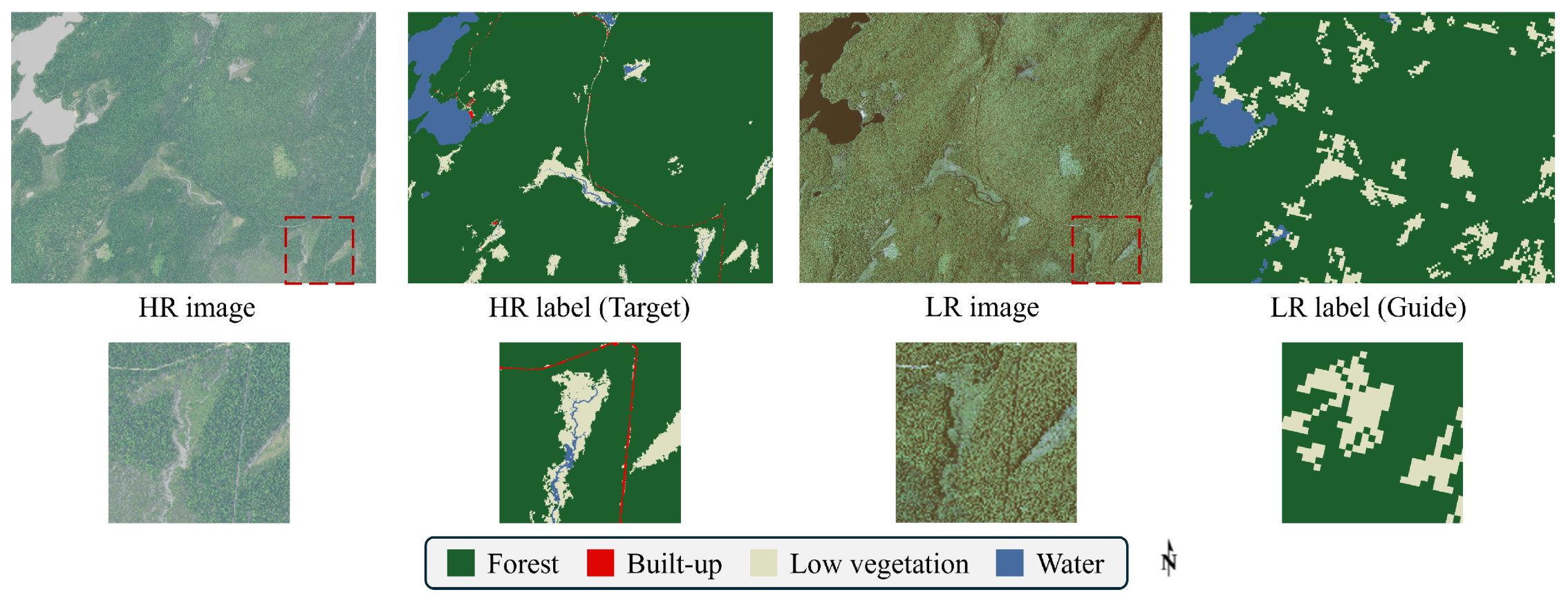
2.1.1. Chesapeake Bay Dataset

The Chesapeake Bay dataset is sampled from the largest estuary in the USA [2], covering 160,000 km² and organized into 732 non-overlapping tiles, where each tile has a size of 6000 × 7500 pixels. The specific data include the following.

• The HR images (1 m/pixel) are from the U.S. Department of Agriculture’s National Agriculture Imagery Program (NAIP). The photos contain four bands of red, green, blue, and near-infrared [37].
• The LR historical annotations (30 m/pixel) are from the USGS’s National Land Cover Database (NLCD) [38], including 16 land cover classes.
• The ground truths (1 m/pixel) are from the Chesapeake Bay Conservancy Land Cover (CCLC) project.

Due to variations in annotation types across the combined datasets, this paper adheres to the standardization guidelines from Paraformer [25] and L2HNet [29]. As shown in

Table 1. Category relations between the HR and LR annotations on the Chesapeake Bay dataset.

Base Annotation	HR Annotation	LR Annotation
Built-up	Roads Buildings Barren	Developed open space Developed low Developed medium Developed high
Tree canopy	Tree canopy	Deciduous forest Evergreen forest Mixed forest Woody wetland
Low vegetation	Low vegetation	Barren land Shrub/scrub Grassland Pasture/hay Cultivated crops Herbaceous wetlands Herbaceous wetlands
Water	Water	Open water

, both high-resolution (HR) and low-resolution (LR) annotations are unified into four fundamental categories for consistent model performance evaluation.

2.1.2. Poland Dataset

The Poland dataset contains 14 provinces of Poland and is organized into 403 non-overlapping tiles, where each tile has a size of 1024 × 1024 pixels. The specific data include the following.

• The HR images (0.25 m and 0.5 m/pixel) are from the LandCover.ai [39] dataset. The images contain three bands of red, green, and blue.
• The LR historical annotations are collected from three types of 10 m land cover data and one type of 30 m data, which are named FROM GLC10 [40], ESA GLC10 [41], ESRI GLC10 [42], and GLC FCS30 [43].
• The HR ground truths are from the OpenEarthMap [44] dataset with five land cover classes.

The standardized mapping for the conversion of HR/LR annotations in the Poland dataset to four fundamental categories is presented in

Table 2. Category relations between the HR and LR annotations on the Poland dataset.

Base Annotation	OpenEarthMap [44]	FROM GLC10 [40]	ESA GLC10 [41]	ESRI GLC10 [42]	GLC FCS30 [43]
Built-up	Developed space Road	Impervious	Built-up	Built area	Impervious surfaces
Tree canopy	Tree	Forest	Tree cover Mangroves	Trees Flooded vegetation	Forest
Low vegetation	Bareland Rangeland Agriculture land	Cropland Grass Shrub Bareland	Shrubland Grassland Cropland Moss and lichen Herbaceous wetland Bare/sparse vegetation	Crops Bare ground Rangeland	Cropland Shrubland Grassland Wetlands Bare areas
Water	Water	Water	Permanent water bodies	Water	Water body

.

2.2. Methods

This study designs an Adaptive Environment Channel Alignment (AECA) module, which performs grouped convolutions on the input image channels to adjust the feature maps’ color distribution and attention weights. We also introduce improvements in the branch fusion part, ensuring better alignment between global and local features. Specifically, the Feature Bridging Mamba (FBMamba) module guides the Transformer’s preference for the sparse global attention map, accelerating the training process while enabling smoother feature fusion.

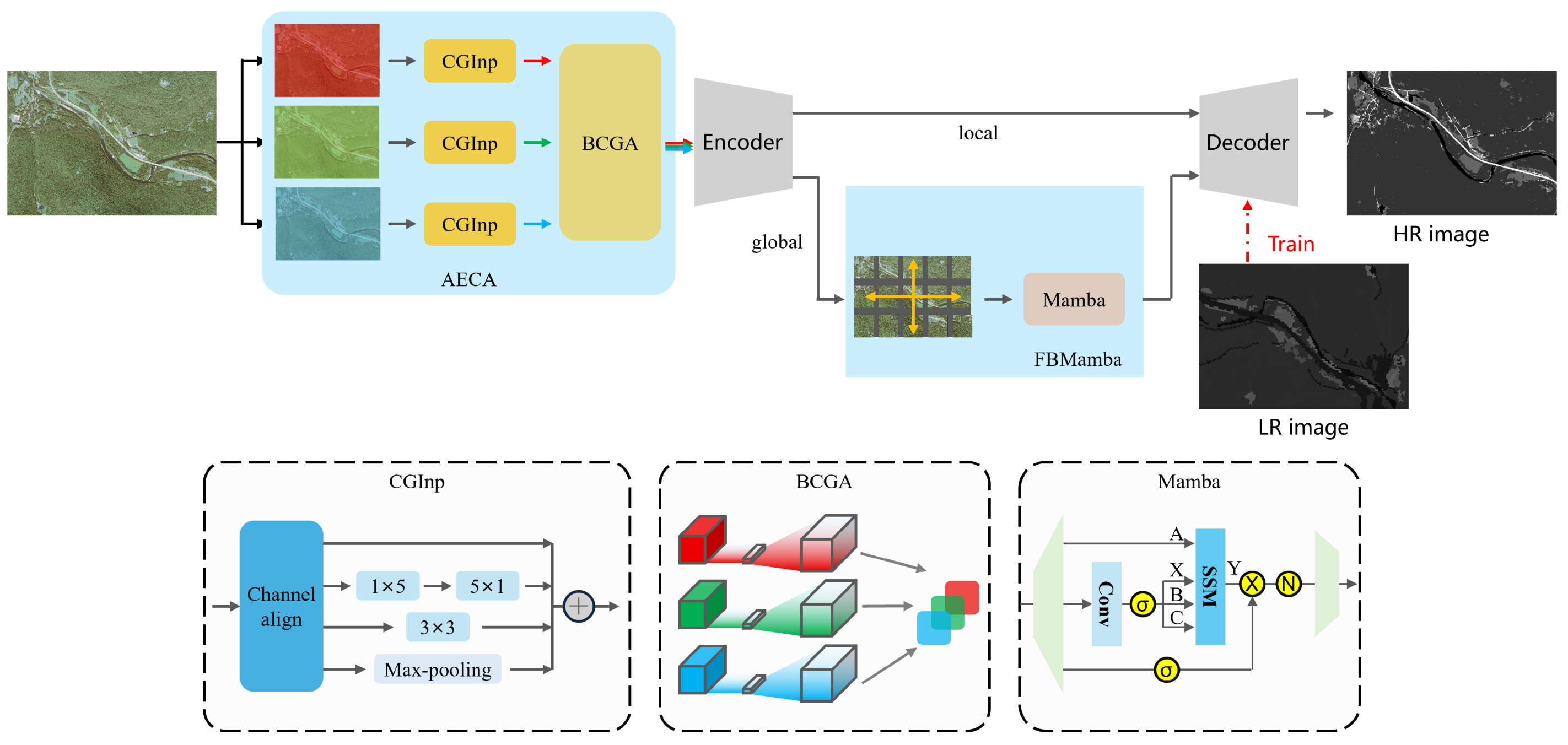
2.2.1. Overall Architecture

As shown in Figure 3, the proposed AECA-FBMamba architecture extends the Paraformer framework [25] through two novel components: (1) the Adaptive Environment Channel Alignment (AECA) module and (2) the Feature Bridging Mamba (FBMamba) middleware. The complete architecture consists of four interconnected components: (i) the AECA-based color space alignment module, (ii) a dual-path encoder, (iii) the FBMamba feature enhancement middleware, and (iv) a hierarchical decoder.

The processing pipeline begins with the AECA module performing grouped convolutions on the input channels to adjust the color distributions and attention weights adaptively. This pre-processing enhances the feature robustness against environmental variations. Next, the aligned features are fed into our dual-path encoder: L2HNet [29] and ViT [14]. L2HNet extracts multi-scale features through progressive spatial downsampling (halving the resolution while doubling the channels), preserving detailed local patterns, and the ViT processes the deepest feature layer to capture rich semantic information through global self-attention. The FBMamba module then bridges these complementary representations, addressing Paraformer’s fusion challenges by providing intermediate receptive fields between the CNN and Transformer that enable smooth feature fusion. Finally, the decoder integrates these enhanced features through a semantic fusion neck and two segmentation heads. The high-throughput CNN branch decoder generates a predicted mask, which is directly used to compute the loss with the LR image labels. This mask is then intersected with the LR image labels to serve as the supervision signal for the Transformer branch decoder, and the loss is computed. The weight for both losses is set to 0.5. This method can screen out uncertain samples and extract reliable information from the LR labels [25].

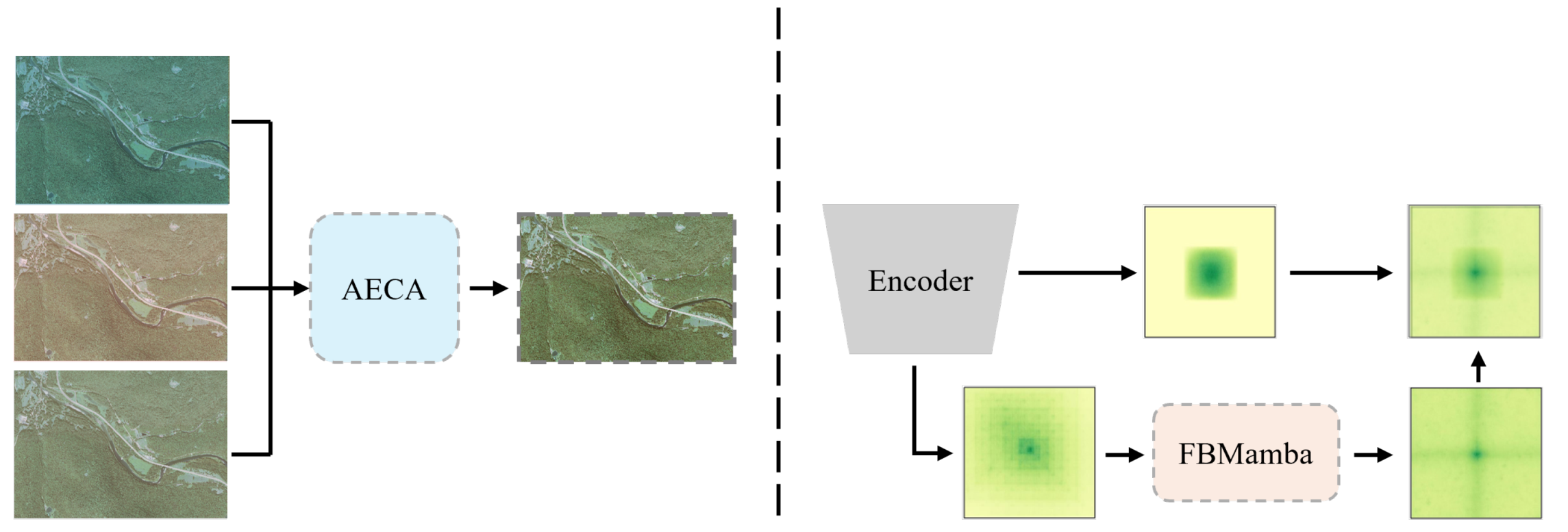
2.2.2. Adaptive Environment Channel Alignment (AECA) Module

In satellite remote sensing scenarios, the atmospheric conditions significantly impact the image quality. Color space selection and optimization represent a fundamental computer vision task. While the RGB color space offers hardware compatibility, its uneven color distribution presents limitations. Environmental factors like the temperature and wind direction introduce optical medium inhomogeneity across regions. Traditional approaches address this by converting RGB to the CIELab space using a standard white-point reference. The CIELab space provides human-perceptual uniformity and device independence after white-point correction, making it ideal for cross-modal color alignment. However, standard white-point acquisition remains challenging in remote sensing applications, and it is weaker in scene versatility compared to adaptive methods.

Recent advances in deep learning have led to growing interest in data-driven color space alignment solutions [45]. Environmental and equipment-induced light attenuation varies non-uniformly across channels, leading to inconsistent color stylization [46]. Previous work has focused on analyzing multi-channel color features through pixel–region comparisons to identify color space variation patterns [45]. These approaches typically employ local receptive field expansion or long-range attention mechanisms on feature maps [47,48]. Notably, most studies have overlooked the fact that intra-channel texture variations remain largely unaffected by surrounding color changes.

Effective feature extraction from individual color channels is essential for robust image analysis. To address this issue, we propose an Automatic Environment Color Alignment (AECA) block that comprehensively identifies color styles across multiple spatial scales and image regions. The AECA architecture operates through two key components: (1) a Channel-Wise Grouped Inception (CGInp) block that performs dedicated feature extraction for each color channel, followed by (2) a Bottleneck Channel Grouped Attention (BCGA) mechanism that intelligently integrates these channel-specific feature representations. This dual-stage design enables a dynamic assessment of each channel’s feature map importance, facilitating optimal channel-wise weighting and information aggregation. This process enhances the feature quality by adaptively combining the most relevant information from each channel. Our AECA implementation preserves the dimensional integrity of the input feature maps, enabling direct plug-and-play integration between the image input and subsequent model components.

The Channel-Wise Grouped Inception (CGInp) module extends the classic Inception architecture [49] by incorporating channel-wise grouped convolutions to enable the isolated processing of color channels. Meanwhile, CGInp maintains the original Inception’s multi-scale feature extraction capabilities through parallel convolutional branches ($1\times 1$, $3\times 3$, and $5\times 5$) and pooling operations. Our CGInp introduces three key enhancements.

• Multi-scale feature preservation: Inherits the Inception module’s fundamental strength in capturing hierarchical visual patterns while adding channel isolation capabilities.
• Enhanced feature diversity: Implicit regularization through grouped convolutions increases feature variation while reducing overfitting risks.
• Channel independence: The decoupled architecture allows flexible input channel configuration without cross-channel parameter interference.

For a standard three-channel input image, the CGInp module (with group number = 3) processes each channel independently through dedicated convolutional branches. As detailed in

Table 3. The detailed construction of our CGInp block in one channel.

Kernel Size	Stride	Output Feature Size	Channel	Group Number
$3\times 3$	1	$224\times 224$	64	64
$1\times 1$	1	$224\times 224$	64	1
$1\times 5$	1, 2	$224\times 224$	64	64
$5\times 1$	2, 1	$224\times 224$	64	64
Max-Pooling	1	$224\times 224$	64	1

, each single-channel processing block maintains spatial dimensions of $224\times 224$, while expanding the channels to 256 through a $1\times 1$ convolution. The expanded features are then divided into four 64-channel feature maps using four parallel operations, $1\times 1$, $3\times 3$, $1\times 5$, and $5\times 1$, and max-pooling operations. The final output concatenates the processed features while maintaining channel isolation during processing. The single-channel transformation can be formally expressed as

$$\mathrm{Output}=f^{11}\left(x\right)+f^{33}\left(f^{11}x)\right)+f^{51}\left(f^{15}\left(f^{11}\left(x\right)\right)\right)+\mathrm{MaxPooling}\left(f^{11}\left(x\right)\right)$$

(1)

where $f^{11}$ indicates the $1\times 1$ convolutional kernel, and x is the input channel. Here, $1\times 1$ convolutional kernels are employed to expand the input from its channel dimension to 64. After this expansion, the $1\times 1$ branch directly outputs the result without performing additional $1\times 1$ convolution operations. This design simplifies the computational flow while maintaining the efficiency of feature transformation. The other branches employ grouped convolutions to extract multi-scale features. This approach divides the input channels into distinct groups, each processed independently through convolutional operations. As a result, the model captures diverse feature representations at varying scales.

As illustrated in Figure 3, the Bottleneck Channel Grouped Attention (BCGA) block weighs the extracted feature maps. On one hand, the BCGA module integrates multi-scale features within each input channel to obtain robust channel feature representations. On the other hand, it expands information exchange across input channels to capture complementary features. The proposed BCGA block can improve the network performance and content representation by considering color-channel-level multi-scale feature fusion attention based on channel compression and reconstruction. The BCGA block utilizes the EXCITATION strategy proposed in SENet to map the feature channel to its weighting coefficients using global average pooling (GAP) [50]. Specifically, the GAP is generated by shrinking each feature map through its spatial dimension:

$$GA{P}_m={\displaystyle \frac{1}{H\times W}}\sum _{i=1}^H\sum _{j=1}^W{F}_m(i,j),m=\{1,2,\dots ,M\}$$

(2)

where $F_m$ is the mth feature map from the CGInp module; $H,W$ are the corresponding height and width of the feature map. The global information channels obtained are first compressed via the fully connected (FC) layer and then restored to their original channel length by another FC layer to emphasize the critical channels. The Softsign function is applied after each FC operation to enhance the model’s nonlinear capacity. The overall computation formula for the BCGA module is presented as follows:

$${\mathrm{BCGA}}_n=Softsign\left(F{C}_2\left(Softsign\left(F{C}_1\left({\mathrm{GAP}}_n\right)\right)\right)\right),n=\{1,2,\dots ,M/N\}$$

(3)

where $F{C}_1,F{C}_2$ are the FC layers; N is the number of input image channels in this paper, but it can also be set to other values, depending on the input channel of the subsequent model.

2.2.3. Feature Bridging Mamba (FBMamba) Block

The state space model (SSM) is the key construction of Mamba [51]. Compared to Transformer-based methods, Mamba exhibits superior representational capabilities in long-sequence modeling while maintaining linear time complexity, providing a notable edge in terms of data handling efficiency. The SSM is typically utilized to represent linear time-invariant systems. It maps a one-dimensional input sequence $x\left(t\right)\in {\mathbb{R}}^L$ to an output sequence $y\left(t\right)\in {\mathbb{R}}^L$ through a latent implicit state $h\left(t\right)\in {\mathbb{R}}^L$, effectively bridging the relationship between inputs and outputs and encapsulating temporal dynamics. Mathematically, the structured state space sequence models (S4) can be formulated as follows:

$$\begin{array}{c}{h}_t=A{h}_{t-1}+B{x}_t\hfill \\ y_t=C^T{h}_t\hfill \end{array}$$

(4)

The S4 models are viewed as a map from $X\to Y$. Mamba-1 was motivated by an SSM-centric point of view, where the selective SSM layer is viewed as a map from $X\to Y$. The parameters $A,B,C$ are regarded as subsidiaries of the SSM input X. The adoption of a discrete-time framework to discretize the ODEs in deep learning applications is common practice [52,53]. This ensures that the model accurately captures the system’s process at discrete intervals $\Delta$. During discretization, the continuous equations that encapsulate the dynamic characteristics of the linear time-invariant system are translated into an equivalent discrete-time representation. Consequently, Equation (4) can be discretized as the following selective scan space state sequential (S6) model:

$$\begin{array}{c}{h}_t=A_t{h}_{t-1}+B_t{x}_t\hfill \\ y_t=C_t^T{h}_t\hfill \\ A_t=e^{\Delta }A\hfill \\ B_t=\Delta B\hfill \\ C_t=C\hfill \end{array}$$

(5)

where $A_t,B_t,C_t$ align the model with the sampling frequency of the discretization step size $\Delta$. These fixed discretization rules serve as the foundation for the SSM’s application, facilitating the seamless incorporation of Mamba into deep learning frameworks. To obtain the essential two-dimensional (2D) visual–spatial information via one-dimensional (1D) sequence modeling, the visual state space model (VSSM) introduces a 2D selective scan mechanism (SS2D). SS2D expands and arranges the image patches in four distinct directions, creating four independent sequences [52]. This quad-directional scanning strategy ensures that each element within the feature map integrates information from all other positions across various directions, generating a global receptive field without increasing the computational complexity. Finally, each feature sequence is processed, culminating in the reconstruction of the 2D feature map by a scan merging operation. Given an input feature z, the output feature $\overline{z}$ of SS2D can be formulated as follows:

$$\begin{array}{c}{z}_i=expand(z,i)\hfill \\ {\overline{z}}_i=S6\left(z_i\right)\hfill \\ \overline{z}=merge\left({\overline{z}}_1,{\overline{z}}_2,{\overline{z}}_3,{\overline{z}}_4\right)\hfill \end{array}$$

(6)

where $i\in \{1,2,3,4\}$ denotes one of the four scanning directions. The functions $expand\left(\right)$ and $merge\left(\right)$ correspond to the operations for scan expanding and scan merging, respectively. The (S6) block serves as the core VSSM operator within SS2D. This operator facilitates interaction between each element within a 1D array and any previously scanned samples via a succinct hidden state.

Current research efforts have focused on directly replacing Transformer architectures with Mamba, with the main emphasis on addressing Mamba’s inherent limitations in high-dimensional image processing [54]. From the attention maps shown in the VMamba paper [52], it can be observed that the feature maps extracted by the Mamba module exhibit the strongest long-range linear dependencies along the scan path. However, in the non-scan direction, its attention is weaker than that of CNNs, which is unfavorable in capturing long-range dependencies in downstream tasks. Transformers, on the other hand, demonstrate sparse attention over a broad region but lack focus and have a slow training process. Mamba can optimize the attention structures of Transformers on sparse graphs.

Based on this observation, this study proposes accelerating the Transformer training process with a Mamba block. In this study, Mamba is directly employed to process the feature flow of the Transformer. During forward propagation, the attention maps generated by the Transformer can provide spatial importance priors, leveraging the Transformer’s global modeling capabilities to mitigate Mamba’s sequential bias. Meanwhile, during backpropagation, Mamba’s stronger feature extraction capabilities are utilized to guide the Transformer’s sparse attention to focus on key information, thereby accelerating the training of the Transformer. To further unify the Mamba and Transformer structures, the Mamba-2 block is adopted [55], which simplifies the Mamba block by removing sequential linear projections. The SSM parameters $\overline{A},\overline{B},\overline{C}$ are produced at the beginning of the block, instead of as a function of the SSM input X. In Mamba-2, the SSD layer is viewed as a map from $X,\overline{A},\overline{B},\overline{C}\to Y$. It therefore makes sense to produce $\overline{A},\overline{B},\overline{C}$ in parallel with a single projection at the beginning of the block:

$$\begin{array}{c}{h}_t=\overline{A}{h}_{t-1}+\overline{B}{x}_t\hfill \\ y_t=\overline{C}T{h}_t\hfill \\ \overline{A},=Softmax\left(CN{N}_A\left(Input\right)\right)\hfill \\ \overline{B}=Softmax\left(CN{N}_B\left(Input\right)\right)\hfill \\ \overline{C}=Softmax\left(CN{N}_C\left(Input\right)\right)\hfill \end{array}$$

(7)

As illustrated in the structure of the FBMamba module in Figure 3, the feature map is first sequentially arranged into feature vectors along four directions, similarly to VMamba [52]. These feature vectors are then passed through a linear layer to adjust the feature dimensions and split into a channel attention branch. In the main branch, the feature vector is further divided: A is directly fed into the SSM, while the remaining portion undergoes a Transformer-like feature transformation using a CNN module, generating vectors X, B, and C, which are also input into the SSM. The output Y of the SSM is reweighted across the feature channels using the channel attention branch vector. Subsequently, the feature dimension is restored to match the input vector dimensions via another linear layer, with activation functions ($\sigma$) and normalization (N) applied, as shown in Figure 3. Finally, the feature vectors from the four directions are recovered by passing them through an activation function and then summing them element-wise.

2.2.4. Evaluation Method

To enable a rigorous assessment of the proposed method’s performance, this study employs a set of evaluative metrics, namely the intersection over union (IoU), mean intersection over union (mIoU), accuracy (Acc), and mean accuracy (mAcc). Specifically, the IoU provides an intuitive and accurate measure of the overlap between the predicted segmentation and the ground truth while maintaining robustness to variations in shape and size. The mIoU is the average of the IoU. The mAcc is the average proportion of pixels where the predicted class matches the ground truth class, and Acc is the proportion relative to the total number of pixels. The formulas for the calculation of the IoU, mIoU, Acc, and mAcc are as follows:

$$\begin{array}{c}{\mathrm{IoU}}_i={\displaystyle \frac{|{\mathrm{Prediction}}_i\cap {\mathrm{GroudTruth}}_i|}{|{\mathrm{Prediction}}_i\cup {\mathrm{GroudTruth}}_i|}}=\sum _{i=1}^k{\displaystyle \frac{p_{ii}}{{\sum }_{j=1}^k{p}_{ij}+{\sum }_{j=1}^k{p}_{ji}-p_{ii}}},\hfill \\ \mathrm{mIoU}={\displaystyle \frac{1}{N}}\sum _{i=1}^N{\mathrm{IoU}}_i\hfill \\ \mathrm{Acc}={\displaystyle \frac{1}{H\times W}}\sum _{i=1}^k{p}_{ii}\hfill \\ \mathrm{mAcc}={\displaystyle \frac{1}{k}}\sum _{i=1}^k{\displaystyle \frac{p_{ii}}{{\sum }_{j=1}^k{p}_{ij}}}\hfill \end{array}$$

(8)

where k is the class number. $p_{ij}$ means that the pixel number of the ground truth (GT) is class i and the prediction is j in the output mask image, and the output mask image size is $H\times W$. The mIoU and mAcc indicate the model’s overall performance and stability on small samples. In contrast, the IoU and Acc primarily reflect the model’s performance under the current data distribution.

2.2.5. Experimental Settings

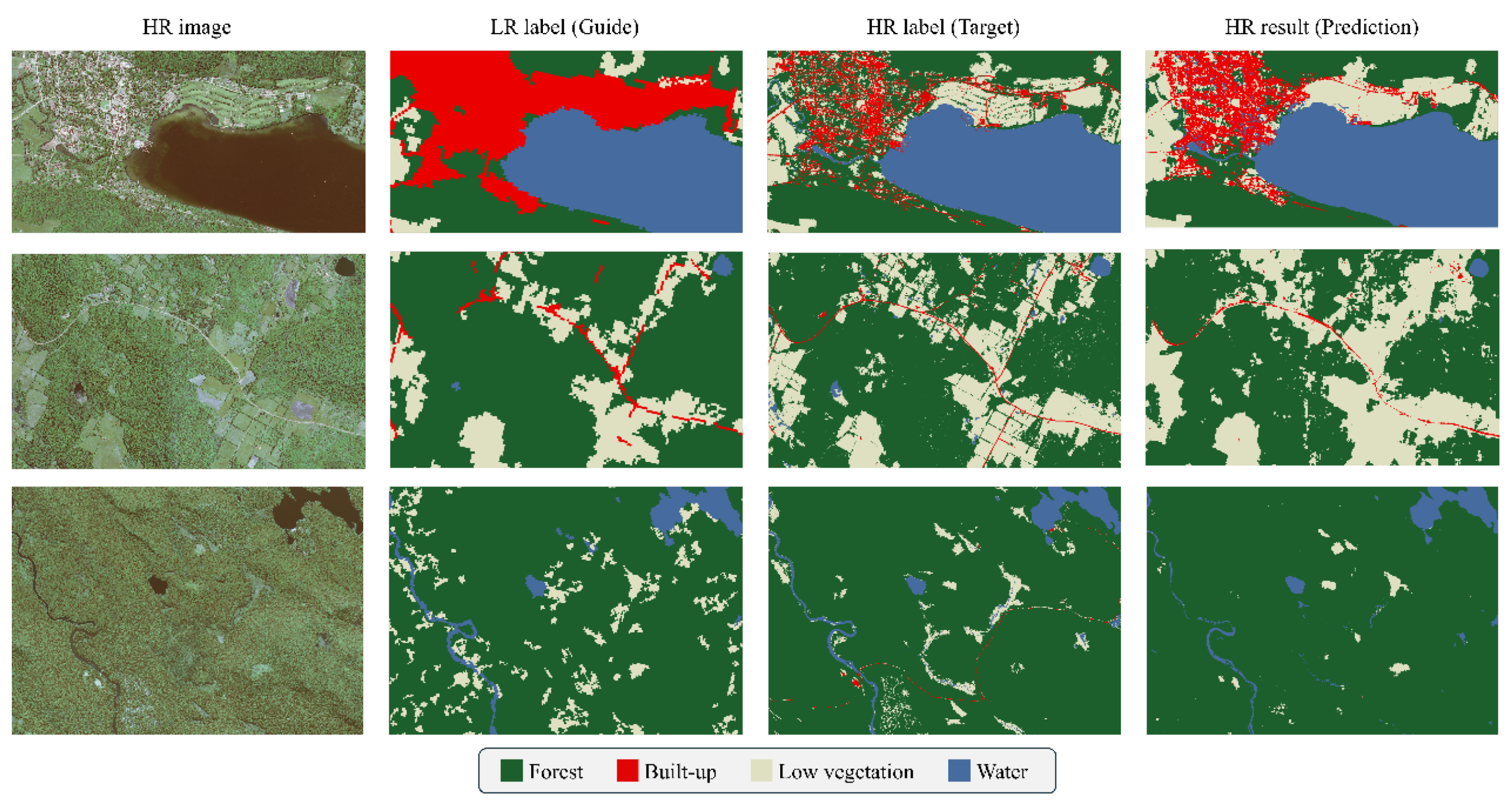
In the experiments, all methods only used HR land cover images as input and LR land cover annotations as the GT. The HR ground references were only used for the accuracy assessment and were not used in the training process. The experiments were implemented using the Python 3.10, CUDA 11.8, and PyTorch 2.1.1 frameworks and were run on a Tesla P100 16 G GPU (Nvidia, Santa Clara, CA, USA) and Intel(R) Xeon(R) Gold 6132 CPU @ 2.60 GHz (Intel, Santa Clara, CA, USA). Our AECA-FBMamba was trained by the AdamW optimizer [56] with a patch size of $224\times 224$ and a batch size of 4. Two types of loss functions were applied in the proposed model, namely cross-entropy (CE) and masked cross-entropy (MCE) loss, and both weights were set to 0.5 [25]. The learning rate was set to 0.01 and decreased by 10% when the loss stopped dropping over eight epochs. After their land cover classes were unified, the evaluation metrics between the results and the HR ground truths were calculated. Additionally, we report the model’s parameter count (mParams), floating-point operations (FLOPs), and frames processed per second (FPS) to comprehensively evaluate its computational efficiency.

3. Results

3.1. Ablation Study

We performed ablation studies using the Chesapeake Bay dataset to evaluate the effectiveness of the optimization components in our AECA-FBMamba model. The visual comparison between the HR annotations and our model’s predictions (as shown in Figure 4) reveals that AECA-FBMamba achieves superior semantic alignment with the HR references compared to the LR annotations. The first row demonstrates that, for built-up areas (shown in red) in the left image region, AECA-FBMamba produces predictions with enhanced texture details and sharper boundary delineation relative to the LR annotations. Similarly, in the second row’s upper-left built-up region, our method generates more spatially continuous predictions than the LR reference. However, as evidenced in the third row, the model fails to reconstruct built-up areas when they are completely missing from the LR annotations. These comparisons reveal our model’s capabilities: it can both correct certain annotation errors and enhance details from LR references, although severe misinformation (as in the third row case) remains challenging. In summary, AECA-FBMamba effectively learns discriminative inter-class features from imperfect LR annotations while producing predictions that more closely approximate the HR quality. The model demonstrates particular strengths in boundary refinement and detail recovery, although its performance remains constrained by the quality of the input annotations.

We conducted ablation experiments to evaluate the contributions of the AECA and FBMamba modules.

Table 4. Ablation results in terms of the FBMamba chunk size on the New York portion of the Chesapeake Bay dataset. The chunk size controls the linear receptive field length in the Mamba module, and this experiment aimed to determine the optimal Mamba receptive field length.

Chunk Size	mIoU	mAcc	Acc	Water IoU	Built-Up IoU	Low Vegetation IoU	Tree IoU
0	67.55	79.68	87.69	85.06	28.71	72.93	83.50
7	68.90	79.73	87.69	85.22	28.13	75.43	86.83
14	70.14	79.51	89.63	85.16	28.90	78.32	88.20
28	70.19	79.58	90.08	86.24	29.53	77.43	87.56

Bold indicates that the model achieves the best performance in the metric, and underline indicates suboptimal performance.

presents the FBMamba block’s ablation study results, where the chunk size corresponds to the linear receptive field length. Using chunk size 0 (the baseline Paraformer model) as a reference, we observed that progressively increasing the chunk size yielded significant improvements in both the mIoU and Acc, with maximum gains of 2.54 and 2.39 percentage points, respectively. However, the mAcc showed minimal variation, with just a 0.17 percentage point difference across configurations. These results demonstrate that the FBMamba module effectively enhances the model’s global and detailed feature representation capabilities, although its influence on the accuracy and stability appears dataset-dependent. The optimal performance occurred at chunk size 28. When comparing chunk sizes 14 and 28, the differences in key metrics (mIoU and mAcc) were marginal (<0.1 percentage points). For practical deployment, we recommend evaluating both configurations and selecting the better-performing option based on the specific application requirements.

We conducted an ablation study to evaluate the impact of the AECA module by selectively removing it from individual channels while maintaining full integration in others. The experimental results are presented in

Table 5. Ablation results regarding the AECA module on the New York portion of the Chesapeake Bay dataset. The red (R), green (G), blue (B), and near-infrared (NIR) channels were analyzed to evaluate the contribution of AECA at each input spectral band.

Channel Name	mIoU	mAcc	Acc	Water IoU	Built-Up IoU	Low Vegetation IoU	Tree IoU
AECA	69.57	81.17	89.08	88.09	29.00	75.81	85.37
- Red (R)	69.13	80.84	88.76	87.53	28.73	75.24	85.00
- Green (G)	69.04	80.77	88.73	87.48	28.91	75.07	84.68
- Blue (B)	69.12	80.85	88.79	87.37	28.88	75.19	85.02
- Near-infrared (NIR)	68.32	80.10	88.35	85.94	28.83	74.26	84.25
Baseline	67.55	79.68	87.69	85.06	28.71	72.93	83.50

Bold indicates that the model achieves the best performance in the metric, and underline indicates suboptimal performance.

. Our experiments reveal that the model consistently outperforms the baseline even when the AECA module is removed from any single channel. The most significant performance degradation occurs when removing the near-infrared channel (average 1.2% drop in accuracy), suggesting that this channel carries unique spectral information not fully captured by RGB channels. On the other hand, a minimal performance variation (<0.5%) occurs when removing the AECA module from any individual RGB channel, indicating strong feature correlation among the visible spectrum channels. The fully integrated AECA model shows consistent improvements of 1.5–2.0 percentage points across all evaluation metrics compared to the baseline, demonstrating its comprehensive enhancement capabilities. This improvement stems from the module’s robust input processing, which effectively optimizes multi-channel feature representation.

The ablation experiment’s results are shown in

Table 6. Ablation results regarding AECA-FBMamba on the New York portion of the Chesapeake Bay dataset. The experiments evaluated the individual contributions of the AECA and FBMamba modules.

Method	mParams	GFLOPs	FPS	mIoU	mAcc	Acc	Water IoU	Built-Up IoU	Low Vegetation IoU	Tree IoU
Baseline	145.40	143.72	15.42	67.55	79.68	87.69	85.06	28.71	72.93	83.50
+ AECA	143.05	116.24	17.76	69.57	81.17	89.08	88.09	29.00	75.81	85.37
+ FBMamba	151.22	102.94	20.22	70.19	79.58	90.08	86.24	29.53	77.43	87.56
Ours	151.55	117.89	17.38	71.91	84.70	89.64	89.64	38.68	76.36	85.94

Bold indicates that the model achieves the best performance in the metric, and underline indicates suboptimal performance.

, with the original Paraformer serving as the baseline. To eliminate performance improvements stemming solely from increased model scale, we reduced the maximum number of channels from 128 (baseline) to 64 when adding new modules. This adjustment ensured comparable model complexity to the baseline when testing individual modified modules. We integrated the proposed blocks separately into the baseline to evaluate their performance. The results demonstrate that the optimization components improve the model’s detection performance, as our AECA-FBMamba network achieves the highest scores of 71.91 mIoU and 84.70 mAcc. Both the AECA and FBMamba blocks outperform the baseline Paraformer. The AECA-enhanced model, combining the CGInp and BCGA, improves the mIoU by 2.02 percentage points and the mAcc by 1.49 compared to the baseline. However, it still falls short of our optimal model by 2.34 mIoU and 3.53 mAcc. In contrast, the FBMamba-integrated model shows stronger performance, increasing the mIoU by 2.64 percentage points but decreasing the mAcc by 0.1 compared to the baseline. Nevertheless, it achieves the highest Acc score of 90.08%. The AECA model delivers a better mAcc result than the FBMamba model, but a lower mIoU and Acc. The AECA module enhances the shallow feature stability and excels in capturing fine details, contributing to its high mAcc. Meanwhile, the FBMamba module smooths global–local information transitions, focusing on semantic-level improvements. Consequently, FBMamba is more affected by the class distribution frequency, leading to high Acc but relatively lower mAcc. The ablation study confirms the proposed optimizations’ effectiveness. By leveraging ViT-Mamba-based frameworks, the AECA-FBMamba model effectively captures local–global positional features, significantly improving the land cover mapping performance. Notably, the mAcc increases by 5.02 percentage points over the baseline, while the built-up class IoU improves by 9.97%, exceeding the sum of the individual module gains. This demonstrates a strong synergistic effect between the two modules.

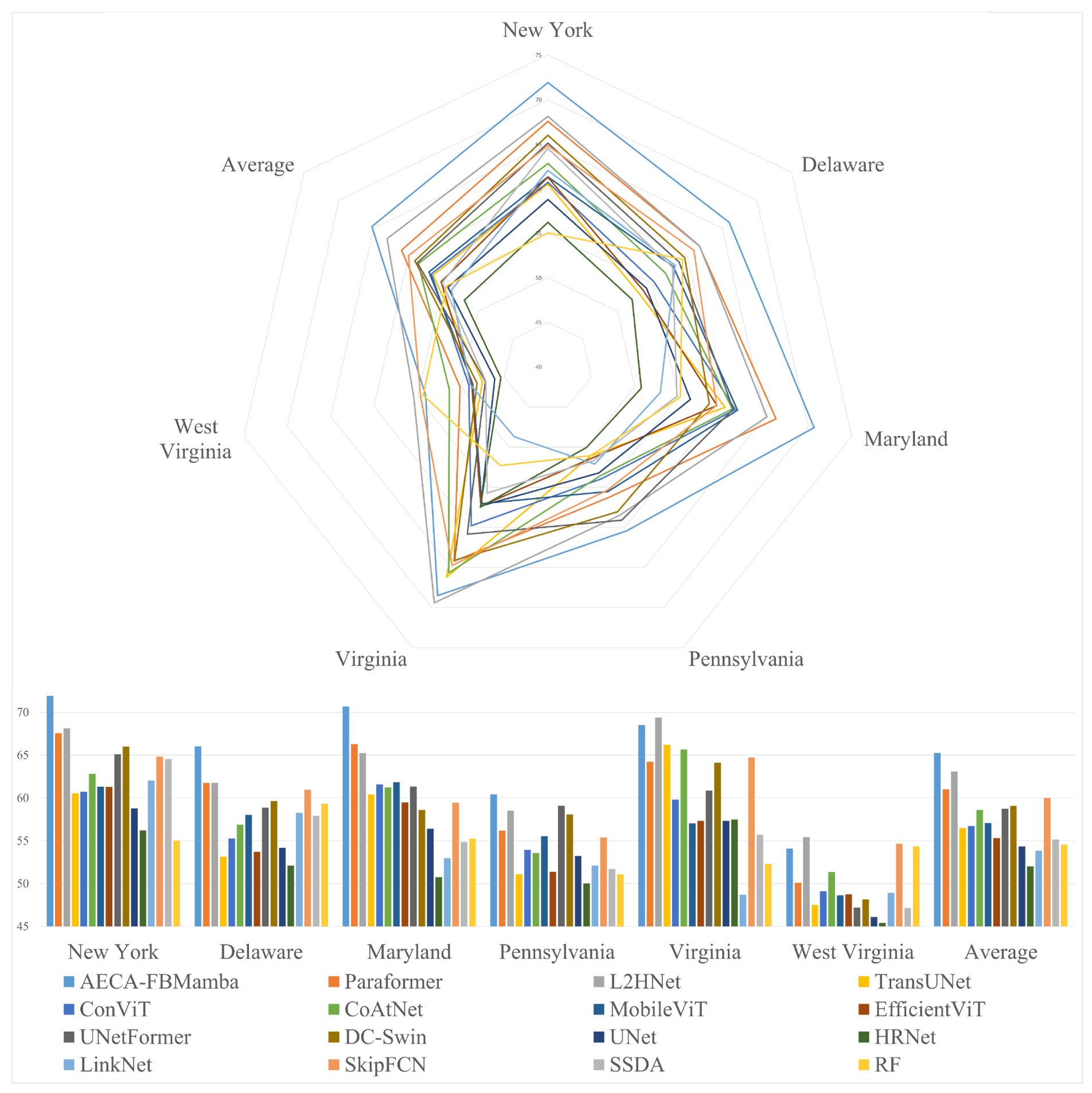
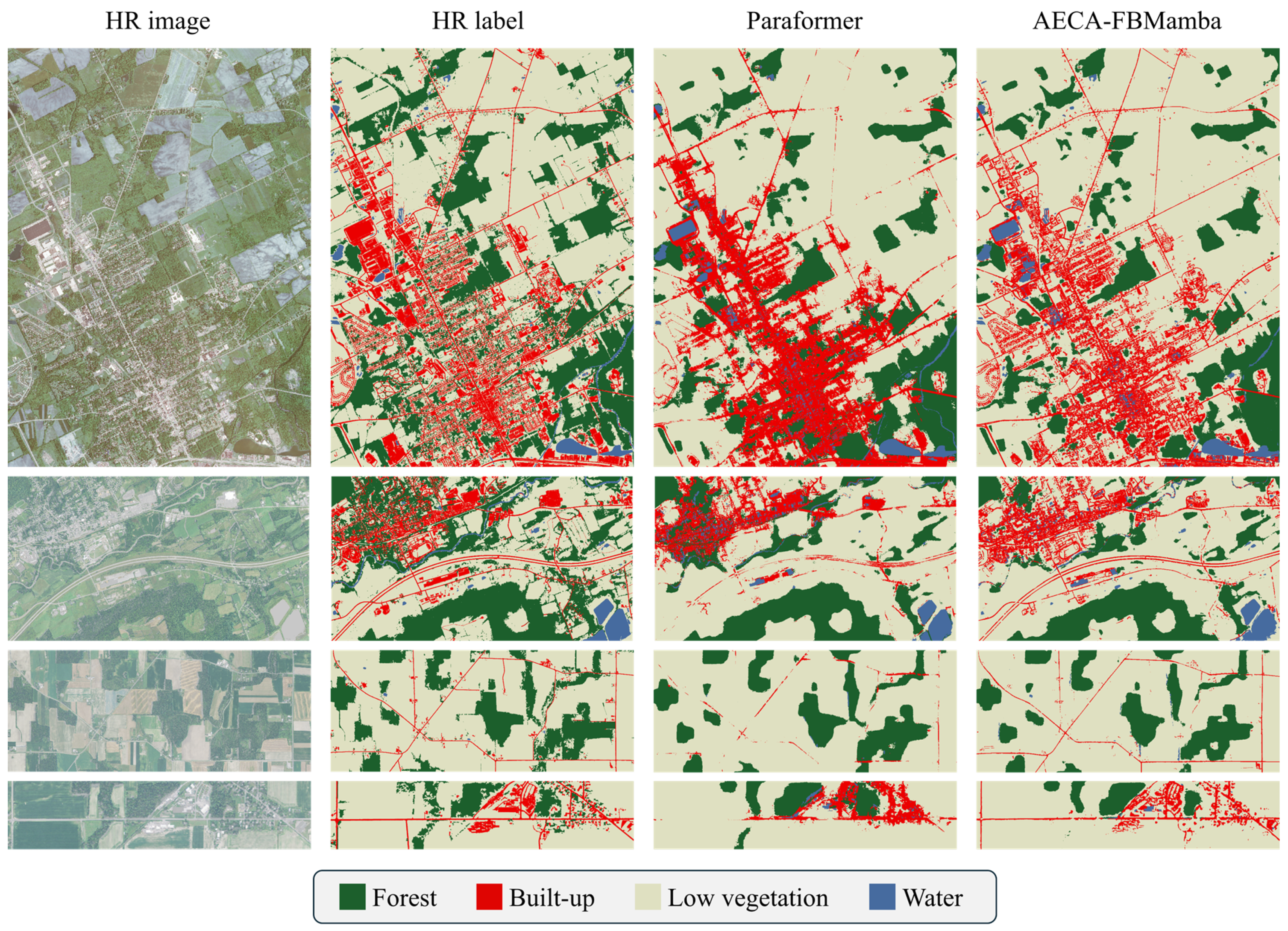
3.2. Comparison with Other Models

To establish comprehensive performance benchmarks, we conducted a rigorous comparative analysis against representative image segmentation approaches. Random forest (RF) [8] is a pixel-to-pixel method widely used in large-scale land cover mapping. UNet [57], HRNet [58], and LinkNet [59] are typical CNN-based semantic segmentation methods that are widely adopted in HR land cover mapping. TransUNet [12], ConViT [20], CoAtNet [60], MobileViT [21], and EfficientViT [19] are CNN–Transformer hybrid methods for semantic segmentation. UNetformer [11] and DC-Swin [18] are dedicated CNN–Transformer methods for remote sensing images. SkipFCN [61] and SSDA [62] are shallow CNN-based methods for the updating of 1 m land cover change maps from 30 m annotations; they won first and second place in the 2021 IEEE GRSS DFC [4]. Paraformer is a state-of-the-art method designed for weakly supervised land cover mapping [25]. Due to computational hardware limitations (specifically GPU memory constraints), the proposed AECA-FBMamba framework and the baseline Paraformer model required the adjustment of the training hyperparameters. Contrary to the original Paraformer configuration, using a batch size of 8, we reduced the batch size to 4. Weakly supervised learning exhibits significantly higher sensitivity to batch size variations than fully supervised paradigms. This modification resulted in performance degradation in Paraformer, which demonstrated an average performance drop of 3.64 percentage points in its mIoU compared to its original value of 64.65 %. All other benchmark models maintained their reported performance metrics when strictly adhering to the training configurations specified in the Paraformer publications.

Table 7. Quantitative comparison of AECA-FBMamba and other methods across six states in the Chesapeake Bay dataset. All methods were trained using 1-m-resolution imagery and 30-m-resolution labels. The mean intersection over union (mIoU, %) was computed between each method’s output and the 1 m ground reference data.

Method	Delaware	New York	Maryland	Pennsylvania	Virginia	West Virginia	Average
AECA-FBMamba	66.02	71.91	70.66	60.43	68.50	54.09	65.27
Paraformer [25]	61.76	67.55	66.28	56.17	64.22	50.10	61.01
L2HNet [29]	61.77	68.12	65.24	58.52	69.39	55.43	63.08
TransUNet [12]	53.15	60.53	60.42	51.08	66.21	47.52	56.49
ConViT [20]	55.26	60.71	61.58	53.94	59.80	49.11	56.73
CoAtNet [60]	56.89	62.83	61.25	53.57	65.67	51.34	58.59
MobileViT [21]	58.03	61.32	61.84	55.53	57.04	48.64	57.07
EfficientViT [19]	53.72	61.28	59.48	51.38	57.34	48.76	55.33
UNetFormer [11]	58.85	65.11	61.34	59.10	60.84	47.20	58.74
DC-Swin [18]	59.65	65.99	58.60	58.06	64.11	48.15	59.09
UNet [57]	54.16	58.79	56.42	53.21	57.34	46.11	54.34
HRNet [58]	52.11	56.21	50.76	50.03	57.48	45.42	52.00
LinkNet [59]	58.27	62.05	52.96	52.11	48.71	48.93	53.84
SkipFCN [61]	60.97	64.83	59.44	55.37	64.72	54.66	60.00
SSDA [62]	57.91	64.54	54.85	51.71	55.71	47.15	55.15
RF [8]	59.35	55.03	55.26	51.07	52.29	54.36	54.56

Bold indicates that the model achieves the best performance in the metric, and underline indicates suboptimal performance.

presents the performance comparisons on the Chesapeake Bay dataset. Our AECA-FBMamba model demonstrates superior performance in Delaware, New York, Maryland, and Pennsylvania based on the quantitative results. In contrast, L2HNet shows better results in Virginia and West Virginia. On average, our AECA-FBMamba achieves the most accurate HR land cover mapping results across the entire area, with an mIoU of 65.27%. This result also surpasses the mIoU of 64.65% reported in the Paraformer paper, where it was trained with a batch size of 8.

However, the best-performing fully supervised method, CoAtNet, ranks only seventh in overall performance. To investigate the differences in the features learned by the models from LR annotations compared to their representation on HR images, we computed the mIoU between HR and LR annotations on the New York dataset. The mIoU of the LR annotations was measured at 61.35%. Among the 16 evaluated methods, only nine approaches (AECA-FBMamba, Paraformer, L2HNet, CoAtNet, UNetFormer, DC-Swin, LinkNet, SkipFCN, and SSDA) outperformed the weakly supervised LR annotation, successfully capturing inter-class discriminative information. Notably, of the nine methods surpassing the LR annotation, all except CoAtNet [60] were weakly supervised segmentation techniques specifically tailored to remote sensing applications. In contrast, the remaining seven algorithms, predominantly classical approaches developed for semantic segmentation tasks, demonstrated performance that was inferior to the LR annotation. Fully supervised models such as HRNet, UNet, EfficientViT, TransUNet, and ConViT, with average mIoUs of 52.00%, 54.34%, 55.35%, 56.49%, and 56.73%, respectively, exhibited excessive dependence on LR annotations, leading to insufficient learning of inter-class differences. This limitation underscores a fundamental challenge in balancing annotation fidelity and the model’s ability to discern nuanced class boundaries. Mismatched training pairs can cause significant misguidance during model training. Excessive attention to fine-grained details in annotations may inadvertently hinder the performance of weakly supervised segmentation.

We further analyzed the performance variation trends of various networks across different datasets to evaluate their stability in diverse scenarios. In Figure 5, the charts depict the performance fluctuations of the models listed in Table 7 across multiple datasets. The degree of fluctuation in the lines reflects the stability of each model. Most methods demonstrate consistent performance across multiple datasets, exhibiting robustness and reliability in diverse scenarios. Notably, RF, LinkNet, and SSDA show extremely poor stability, with their performance being highly sensitive to variations in dataset scenes. Due to the lack of deep-level feature representation and global contextual information, LinkNet, SSDA, and RF achieve average mIoUs of 53.84%, 55.15%, and 54.56%, respectively. Consequently, the relative ranking of these methods frequently shifts depending on the dataset. Although these approaches achieved leading performance on the New York dataset, their inconsistency across other datasets highlights a significant limitation in their generalizability. In contrast, our proposed AECA-FBMamba model achieves superior performance in most scenarios while maintaining high consistency. This demonstrates the model’s robustness and adaptability across varying conditions.

In Figure 6, we present the partial visualization results for AECA-FBMamba compared to the state-of-the-art (SOTA) Paraformer. From Table 6, it is evident that the performance gap between our AECA-FBMamba and Paraformer is most pronounced for the built-up class. Additionally, the built-up class exhibits the lowest IoU among all classes, making its visualization a key focus of this study. In this figure, we showcase the results across multiple scales and different regions. From the first row of the image, which depicts a large built-up area, and the fourth row, which shows a small, sparse built-up region, it is clear that AECA-FBMamba achieves better fine-grained segmentation for large-area regions compared to Paraformer. Furthermore, examining the second row, which highlights a curved region in the middle, and the third row, which focuses on sparse built-up lines, AECA-FBMamba demonstrates a superior ability to predict continuous lines. This indicates that the model excels in integrating long-range features with detailed features, leading to more accurate and coherent predictions.

Comparison on the Poland dataset: In the experiments with the Poland dataset, all methods were used to produce 0.25/0.5 m land cover maps of 14 provinces in Poland by exploiting four LR annotations separately. These LR annotations included 10 m FROM GLC10 [40], ESA GLC10 [41], ESRI GLC10 [42], and GLC FCS30 [43]. As shown in

Table 8. The quantitative comparison on the Poland dataset. The mIoUs (%) of SECA-FBMamba and other methods that were trained with three types of 10 m annotations (i.e., FROMGLC10, ESAGLC10, and EsriGLC10) and one type of 30 m annotation (i.e., GLCFCS30) are demonstrated.

		mIoU (%) of Different Methods
Max Gap	LR Annotation	AECA-FBMamba	Paraformer [25]	L2HNet [29]	TransUNet [12]	HRNet [58]	SkipFCN [61]
	FEOM_CLC10	56.96	53.49	50.15	38.44	43.66	27.14
40×	ESA_GLC10	55.55	52.14	52.13	35.58	49.81	28.34
	Esri_GLC10	55.44	52.05	50.78	26.20	41.46	23.67
120×	GLC_FCS30	49.71	46.42	43.62	26.20	41.46	23.67

Bold indicates that the model achieves the best performance in the metric, and underline indicates suboptimal performance.

, AECA-FBMamba was compared with five representative methods (i.e., weakly supervised, CNN–Transformer, CNN-based, and pixel-to-pixel approaches) in a more extreme geospatial mismatch.

Compared with the state-of-the-art method, AECA-FBMamba shows an increase in its mIoU of 3.47%, 3.41%, and 3.39% when exploiting 10 m annotations with a resolution gap of $40\times$. When resolving 30 m annotations with a maximum resolution gap of $120\times$, AECA-FBMamba has an mIoU of 49.71%, with an increase of 3.29% compared with Paraformer [25]. The typical CNN-based method, HRNet [58], has an average mIoU of 46.71% among the 10 m cases and 41.46% in the 30 m case. SkipFCN [61] has the lowest mIoU among all methods, which shows its difficulty in dealing with extremely mismatched situations.

4. Discussion

4.1. Reducing the Focus on Details Benefits Weakly Supervised Training

In the design of Paraformer, we observed an unusual architectural decision. Specifically, it abandons the multi-scale feature fusion perception between the semantic and detail branches—a structure that has been proven in HRNet [58] to effectively enhance the performance of fully supervised segmentation models. Based on this observation, we propose the following hypothesis: in weakly supervised segmentation tasks, decoder-side modifications tend to introduce negative optimization effects due to the low-quality supervisory signals, particularly when emphasizing detailed feature refinement. Weakly supervised approaches typically employ one of three strategies: (1) designing softly evaluated loss functions [63,64], (2) directly analyzing pixel-wise correlations to establish new semantic relationships that can be propagated to unlabeled regions [65,66], or (3) combining multiple weak supervision sources to obtain enhanced supervisory signals [67]. These methods either attenuate the perception of fine-grained details within labels or construct detail awareness through alternative approaches, which aligns with our proposed hypothesis. Guided by this hypothesis, the enhancement modules that we propose are strategically positioned either at the front end of the encoder or at the junction between the encoder and decoder. This design choice aims to mitigate the adverse impacts of low-quality annotations while ensuring robust feature extraction and stable model performance.

Decoder-Side Modification Analysis

To validate this hypothesis, we implemented three fully supervised prevalent segmentation methods (UNet [57], HRNet [58], and TransUNet [12]) on the Chesapeake Bay New York dataset. As shown in Table 7, all these fully supervised segmentation methods caused performance degradation in Paraformer. Compared to UNet [57] and TransUNet [12], the Transformer module for the extraction of semantic information brought a 2.15-percentage-point improvement in the mIoU. Conversely, HRNet [58], which incorporates multi-scale feature fusion and interaction strategies compared to UNet, resulted in a 2.34-percentage-point decrease in the mIoU. HRNet, with the most boundary refinement, showed the most severe penalty. This empirical evidence supports our hypothesis that detail-focused decoder modifications exacerbate error propagation in weakly supervised settings.

We further incorporated several detail-enhancing modules (CGA [68], MSAA [69], and DA [12]), commonly employed in semantic segmentation decoders, into the Paraformer baseline network. We also redesigned the RPBlock used in the Paraformer CNN branch by replacing standard $n\times n$ convolutions with sequential $1\times n$ and $n\times 1$ linear convolution pairs (the linear convolutional combination exhibits a preference for perceiving linear features [70]). The experimental results, summarized in

Table 9. Comparison result on Chesapeake Bay New York dataset with detailed information enhancement blocks.

Method	mIoU	mAcc	Acc	Water IoU	Built-Up IoU	Low Vegetation IoU	Tree IoU
Baseline	67.55	79.68	87.69	85.06	28.71	72.93	83.50
+ CGA [68]	64.07	78.05	82.19	81.38	34.90	65.85	74.17
+ MSAA [69]	65.81	76.05	89.05	85.92	14.90	75.73	86.71
+ DA [12]	61.88	69.00	89.67	84.22	12.47	76.10	87.20
+ RPLinear block [29]	66.46	76.08	88.57	80.97	24.15	75.57	85.16

Bold indicates that the model achieves the best performance in the metric, and underline indicates suboptimal performance.

, indicated that these modifications generally led to a decline in Paraformer’s performance and it exhibited unstable preferences across multiple categories. This outcome underscores the importance of carefully balancing the level of detail in annotation usage within weakly supervised frameworks, as overemphasis on fine-grained features can undermine the effectiveness of the baseline network. These findings contribute valuable insights into the design principles for weakly supervised segmentation algorithms, particularly in the context of remote sensing applications.

Our findings suggest that the LR annotations introduce inherent resolution gaps in weakly supervised land cover mapping. As a result, detail enhancement blocks at decoder stages amplify annotation inaccuracies. On the contrary, feature stabilization at encoder stages proves more effective. This drives our architecture design to prioritize encoder-side feature normalization rather than decoder-side detail enhancement.

4.2. Synergistic Integration of Transformer and Mamba

We conducted experiments on hybrid configurations of ViT [14] and FBMamba architectures to evaluate their complementary advantages. As shown in

Table 10. Ablation study on the number settings of ViT and our FBMamba blocks.

ViT Num	FBMamba Num	mParams	GFLOPs	FPS	mIoU	mAcc	Acc
12	0	145.40	143.72	15.42	67.55	79.68	89.69
12	1	151.55	117.89	17.38	71.91	84.70	89.64
12	2	160.06	119.54	17.11	71.75	82.03	89.80
11	1	144.47	116.44	17.57	70.61	79.69	89.70
11	2	152.97	118.09	17.37	67.80	79.11	89.53
10	1	137.38	114.99	17.92	67.00	79.98	89.83
10	2	145.88	116.64	17.75	61.33	69.66	89.54

Bold indicates that the model achieves the best performance in the metric, and underline indicates suboptimal performance.

, multiple implementations were tested. On one hand, we replaced ViT blocks with FBMamba blocks. Starting from the Paraformer integrated with our AECA module (12 ViT and 0 FBMamba layers: a pure Vision Transformer architecture with 12 standard layers), we incrementally replaced two ViT blocks with FBMamba blocks (10 ViT and 2 FBMamba: insertion of two FBMamba layers while retaining all original ViT components). On the other hand, we explored additional FBMamba blocks to identify the configuration that yielded the best model performance. The experimental results demonstrate that the combination of 12 ViT modules and 1 FBMamba module achieves the best performance, with an mIoU of 71.91 and an mAcc of 84.70. The combination of 11 ViT modules and 1 FBMamba module achieves suboptimal performance. Notably, all models utilizing two FBMamba modules performed worse than their counterparts with only one FBMamba module under the same conditions. Additionally, reducing the number of ViT modules consistently degrades the model performance, and the fewer ViT modules there are, the greater the performance drop caused by adding a second FBMamba module.

When comparing the performance of a model with 11 ViT modules and 1 FBMamba module to one with only 12 ViT modules, replacing one ViT module with an FBMamba module improved the performance. However, this improvement diminishes when more ViT modules are replaced. These findings validate the feature smoothing transition theory proposed in this paper. The Mamba module can serve as a bridge for feature transformation between the ViT and CNN, and this smoothing process does not need to be repeated. Furthermore, the metric Acc supports the aforementioned conclusions. The maximum difference in the Acc values among all models in Table 10 is 0.30%. This suggests that the Mamba module does not significantly impact the model’s pixel-wise classification ability. However, the increase in mIoU indicates an improvement in the model’s capability to delineate category-specific regions accurately. The FBMamba module proposed in this paper effectively guides the model’s perception toward areas that are more relevant to the target class categories.

5. Conclusions

This paper proposes a weakly supervised framework for high-resolution image segmentation under low-quality supervision, addressing the precision and robustness limitations of existing methods through two key innovations: cross-modal color space alignment and a semantic detail decoupling design. The Adaptive Environment Channel Alignment (AECA) module is proposed to enable adaptive optimization across different color spaces. This enhances the robustness of cross-domain segmentation models in weakly supervised scenarios by improving feature extraction under varying environmental conditions. The Feature Bridging Mamba (FBMamba) module is designed to streamline training by guiding sparse attention mechanisms with linear scanning, thereby focusing computational resources on key regions. This approach not only accelerates convergence but also ensures the smoother integration of global semantic and local detailed features. Additionally, this study highlights that reducing the emphasis on fine-grained details can significantly benefit weakly supervised training, as overly detailed representations may introduce noise or misalignment when paired with low-quality annotations. Future research could explore annotation-insensitive approaches to detail prediction. The proposed framework demonstrates strong practical applicability in domains such as land cover mapping and agricultural monitoring, showcasing its potential for real-world implementation. By bridging the gap between low-quality supervision and high-resolution outputs, this work provides a robust solution for large-scale geospatial analysis, paving the way for further advancements in weakly supervised remote sensing applications.

References

1. Cihlar, J. Land cover mapping of large areas from satellites: Status and research priorities. Int. J. Remote Sens. 2000, 21, 1093–1114. [Google Scholar] [CrossRef]
2. Robinson, C.; Hou, L.; Malkin, K.; Soobitsky, R.; Czawlytko, J.; Dilkina, B.; Jojic, N. Large Scale High-Resolution Land Cover Mapping With Multi-Resolution Data. In Proceedings of the 2019 IEEE/CVF Conference on Computer Vision and Pattern Recognition (CVPR), Long Beach, CA, USA, 15–20 June 2019; pp. 12718–12727. [Google Scholar] [CrossRef]
3. Girard, N.; Smirnov, D.; Solomon, J.; Tarabalka, Y. Polygonal Building Extraction by Frame Field Learning. In Proceedings of the 2021 IEEE/CVF Conference on Computer Vision and Pattern Recognition (CVPR), Nashville, TN, USA, 20–25 June 2021; pp. 5887–5896. [Google Scholar] [CrossRef]
4. Li, Z.; Lu, F.; Zhang, H.; Tu, L.; Li, J.; Huang, X.; Robinson, C.; Malkin, K.; Jojic, N.; Ghamisi, P.; et al. The Outcome of the 2021 IEEE GRSS Data Fusion Contest - Track MSD: Multitemporal Semantic Change Detection. IEEE J. Sel. Top. Appl. Earth Obs. Remote Sens. 2022, 15, 1643–1655. [Google Scholar] [CrossRef]
5. Tong, X.Y.; Xia, G.S.; Lu, Q.; Shen, H.; Li, S.; You, S.; Zhang, L. Land-cover classification with high-resolution remote sensing images using transferable deep models. Remote Sens. Environ. 2020, 237, 111322. [Google Scholar] [CrossRef]
6. Janga, B.; Asamani, G.P.; Sun, Z.; Cristea, N. A Review of Practical AI for Remote Sensing in Earth Sciences. Remote Sens. 2023, 15, 4112. [Google Scholar] [CrossRef]
7. Friedl, M.; Brodley, C. Decision tree classification of land cover from remotely sensed data. Remote Sens. Environ. 1997, 61, 399–409. [Google Scholar] [CrossRef]
8. Chan, J.C.W.; Paelinckx, D. Evaluation of Random Forest and Adaboost tree-based ensemble classification and spectral band selection for ecotope mapping using airborne hyperspectral imagery. Remote Sens. Environ. 2008, 112, 2999–3011. [Google Scholar] [CrossRef]
9. Shi, D.; Yang, X. Support Vector Machines for Land Cover Mapping from Remote Sensor Imagery; Springer Remote Sensing/Photogrammetry; Springer: Dordrecht, The Netherlands, 2015; pp. 265–279. [Google Scholar] [CrossRef]
10. Luo, M.; Ji, S. Cross-spatiotemporal land-cover classification from VHR remote sensing images with deep learning based domain adaptation. ISPRS J. Photogramm. Remote Sens. 2022, 191, 105–128. [Google Scholar] [CrossRef]
11. Wang, L.; Li, R.; Zhang, C.; Fang, S.; Duan, C.; Meng, X.; Atkinson, P.M. UNetFormer: A UNet-like transformer for efficient semantic segmentation of remote sensing urban scene imagery. ISPRS J. Photogramm. Remote Sens. 2022, 190, 196–214. [Google Scholar] [CrossRef]
12. Chen, J.; Lu, Y.; Yu, Q.; Luo, X.; Adeli, E.; Wang, Y.; Lu, L.; Yuille, A.L.; Zhou, Y. TransUNet: Transformers Make Strong Encoders for Medical Image Segmentation. arXiv 2021, arXiv:2102.04306. [Google Scholar]
13. Liu, Z.; Lin, Y.; Cao, Y.; Hu, H.; Wei, Y.; Zhang, Z.; Lin, S.; Guo, B. Swin Transformer: Hierarchical Vision Transformer using Shifted Windows. In Proceedings of the 18th IEEE/CVF International Conference on Computer Vision (ICCV), Montreal, QC, Canada, 10–17 October 2021; pp. 9992–10002. [Google Scholar] [CrossRef]
14. Dosovitskiy, A.; Beyer, L.; Kolesnikov, A.; Weissenborn, D.; Zhai, X.; Unterthiner, T.; Dehghani, M.; Minderer, M.; Heigold, G.; Gelly, S.; et al. An Image is Worth 16x16 Words: Transformers for Image Recognition at Scale. arXiv 2021, arXiv:2010.11929. [Google Scholar]
15. Chen, K.; Zou, Z.; Shi, Z. Building Extraction from Remote Sensing Images with Sparse Token Transformers. Remote Sens. 2021, 13, 4441. [Google Scholar] [CrossRef]
16. Li, J.; He, W.; Cao, W.; Zhang, L.; Zhang, H. UANet: An Uncertainty-Aware Network for Building Extraction From Remote Sensing Images. IEEE Trans. Geosci. Remote Sens. 2024, 62, 5608513. [Google Scholar] [CrossRef]
17. Sun, Z.; Zhou, W.; Ding, C.; Xia, M. Multi-Resolution Transformer Network for Building and Road Segmentation of Remote Sensing Image. ISPRS Int. J. Geo-Inf. 2022, 11, 165. [Google Scholar] [CrossRef]
18. Wang, L.; Li, R.; Duan, C.; Zhang, C.; Meng, X.; Fang, S. A novel transformer based semantic segmentation scheme for fine-resolution remote sensing images. IEEE Geosci. Remote Sens. Lett. 2022, 19, 6506105. [Google Scholar] [CrossRef]
19. Cai, H.; Li, J.; Hu, M.; Gan, C.; Han, S. EfficientViT: Lightweight Multi-Scale Attention for High-Resolution Dense Prediction. In Proceedings of the 2023 IEEE/CVF International Conference on Computer Vision (ICCV), Paris, France, 1–6 October 2023; pp. 17256–17267. [Google Scholar] [CrossRef]
20. d’Ascoli, S.; Touvron, H.; Leavitt, M.L.; Morcos, A.S.; Biroli, G.; Sagun, L. ConViT: Improving vision transformers with soft convolutional inductive biases*. J. Stat. Mech. Theory Exp. 2022, 2022, 114005. [Google Scholar] [CrossRef]
21. Mehta, S.; Rastegari, M. MobileViT: Light-weight, General-purpose, and Mobile-friendly Vision Transformer. arXiv 2021, arXiv:2110.02178. [Google Scholar]
22. Kirillov, A.; Mintun, E.; Ravi, N.; Mao, H.; Rolland, C.; Gustafson, L.; Xiao, T.; Whitehead, S.; Berg, A.C.; Lo, W.Y.; et al. Segment Anything. arXiv 2023, arXiv:2304.02643. [Google Scholar]
23. Wu, Q.; Osco, L.P. samgeo: A Python package for segmenting geospatial data with the Segment Anything Model (SAM). J. Open Source Softw. 2023, 8, 5663. [Google Scholar] [CrossRef]
24. Osco, L.P.; Wu, Q.; de Lemos, E.L.; Gonçalves, W.N.; Ramos, A.P.M.; Li, J.; Marcato, J. The Segment Anything Model (SAM) for remote sensing applications: From zero to one shot. Int. J. Appl. Earth Obs. Geoinf. 2023, 124, 103540. [Google Scholar] [CrossRef]
25. Li, Z.; He, W.; Li, J.; Lu, F.; Zhang, H. Learning without Exact Guidance: Updating Large-Scale High-Resolution Land Cover Maps from Low-Resolution Historical Labels. In Proceedings of the 2024 IEEE/CVF Conference on Computer Vision and Pattern Recognition (CVPR), Los Alamitos, CA, USA, 17–21 June 2024; pp. 27717–27727. [Google Scholar] [CrossRef]
26. Cao, Y.; Huang, X. A coarse-to-fine weakly supervised learning method for green plastic cover segmentation using high-resolution remote sensing images. ISPRS J. Photogramm. Remote Sens. 2022, 188, 157–176. [Google Scholar] [CrossRef]
27. Malkin, K.; Robinson, C.; Hou, L.; Jojic, N. Label super-resolution networks. In Proceedings of the International Conference on Learning Representations, New Orleans, LA, USA, 6–9 May 2019. [Google Scholar]
28. Chen, Y.; Zhang, G.; Cui, H.; Li, X.; Hou, S.; Ma, J.; Li, Z.; Li, H.; Wang, H. A novel weakly supervised semantic segmentation framework to improve the resolution of land cover product. ISPRS J. Photogramm. Remote Sens. 2023, 196, 73–92. [Google Scholar] [CrossRef]
29. Li, Z.; Zhang, H.; Lu, F.; Xue, R.; Yang, G.; Zhang, L. Breaking the resolution barrier: A low-to-high network for large-scale high-resolution land-cover mapping using low-resolution labels. ISPRS J. Photogramm. Remote Sens. 2022, 192, 244–267. [Google Scholar] [CrossRef]
30. He, K.; Zhang, X.; Ren, S.; Sun, J. Deep Residual Learning for Image Recognition. In Proceedings of the 2016 IEEE Conference on Computer Vision and Pattern Recognition (CVPR), Las Vegas, NV, USA, 27–30 June 2016; pp. 770–778. [Google Scholar] [CrossRef]
31. Kirillov, A.; Girshick, R.; He, K.; Dollar, P.; Soc, I.C. Panoptic Feature Pyramid Networks. In Proceedings of the 32nd IEEE/CVF Conference on Computer Vision and Pattern Recognition (CVPR), Long Beach, CA, USA, 15–20 June 2019; pp. 6392–6401. [Google Scholar] [CrossRef]
32. Long, J.; Shelhamer, E.; Darrell, T. Fully Convolutional Networks for Semantic Segmentation. In Proceedings of the IEEE Conference on Computer Vision and Pattern Recognition (CVPR), Boston, MA, USA, 7–12 June 2015; pp. 3431–3440. [Google Scholar] [CrossRef]
33. Zhu, K.; Xiong, N.N.; Lu, M. A Survey of Weakly-supervised Semantic Segmentation. In Proceedings of the 2023 IEEE 9th Intl Conference on Big Data Security on Cloud (BigDataSecurity), IEEE Intl Conference on High Performance and Smart Computing, (HPSC) and IEEE Intl Conference on Intelligent Data and Security (IDS), New York, NY, USA, 6–8 May 2023; pp. 10–15. [Google Scholar] [CrossRef]
34. Vincenzi, S.; Porrello, A.; Buzzega, P.; Cipriano, M.; Fronte, P.; Cuccu, R.; Ippoliti, C.; Conte, A.; Calderara, S. The color out of space: Learning self-supervised representations for earth observation imagery. In Proceedings of the 2020 25th International Conference on Pattern Recognition (ICPR), Milan, Italy, 10–15 January 2020; pp. 3034–3041. [Google Scholar]
35. Yang, Z.; Cao, S.; Aibin, M. Beyond sRGB: Optimizing Object Detection with Diverse Color Spaces for Precise Wildfire Risk Assessment. Remote Sens. 2025, 17, 1503. [Google Scholar] [CrossRef]
36. Yang, H.; Kong, J.; Hu, H.; Du, Y.; Gao, M.; Chen, F. A Review of Remote Sensing for Water Quality Retrieval: Progress and Challenges. Remote Sens. 2022, 14, 1770. [Google Scholar] [CrossRef]
37. Maxwell, A.E.; Warner, T.A.; Vanderbilt, B.C.; Ramezan, C.A. Land Cover Classification and Feature Extraction from National Agriculture Imagery Program (NAIP) Orthoimagery: A Review. Photogramm. Eng. Remote Sens. 2017, 83, 737–747. [Google Scholar] [CrossRef]
38. Wickham, J.; Stehman, S.V.; Sorenson, D.G.; Gass, L.; Dewitz, J.A. Thematic accuracy assessment of the NLCD 2016 land cover for the conterminous United States. Remote Sens. Environ. 2021, 257, 112357. [Google Scholar] [CrossRef]
39. Boguszewski, A.; Batorski, D.; Ziemba-Jankowska, N.; Dziedzic, T.; Zambrzycka, A. LandCover.ai: Dataset for Automatic Mapping of Buildings, Woodlands, Water and Roads from Aerial Imagery. In Proceedings of the 2021 IEEE/CVF Conference on Computer Vision and Pattern Recognition Workshops (CVPRW), Nashville, TN, USA, 19–25 June 2021. [Google Scholar] [CrossRef]
40. Gong, P.; Liu, H.; Zhang, M.; Li, C.; Wang, J.; Huang, H.; Clinton, N.; Ji, L.; Li, W.; Bai, Y.; et al. Stable classification with limited sample: Transferring a 30-m resolution sample set collected in 2015 to mapping 10-m resolution global land cover in 2017. Sci. Bull. 2019, 64, 370–373. [Google Scholar] [CrossRef]
41. Van De Kerchove, R.; Zanaga, D.; Keersmaecker, W.; Souverijns, N.; Wevers, J.; Brockmann, C.; Grosu, A.; Paccini, A.; Cartus, O.; Santoro, M.; et al. ESA WorldCover: Global land cover mapping at 10 m resolution for 2020 based on Sentinel-1 and 2 data. In Proceedings of the AGU Fall Meeting Abstracts, New Orleans, LA, USA, 13–17 December 2021; Volume 2021, pp. GC45I–0915. [Google Scholar]
42. Karra, K.; Kontgis, C.; Statman-Weil, Z.; Mazzariello, J.C.; Mathis, M.; Brumby, S.P. Global land use/land cover with Sentinel 2 and deep learning. In Proceedings of the 2021 IEEE International Geoscience and Remote Sensing Symposium IGARSS, Brussels, Belgium, 11–16 July 2021; pp. 4704–4707. [Google Scholar] [CrossRef]
43. Zhang, X.; Liu, L.; Chen, X.; Gao, Y.; Xie, S.; Mi, J. GLC_FCS30: Global land-cover product with fine classification system at 30 m using time-series Landsat imagery. Earth Syst. Sci. Data 2021, 13, 2753–2776. [Google Scholar] [CrossRef]
44. Xia, J.; Yokoya, N.; Adriano, B.; Broni-Bediako, C. OpenEarthMap: A Benchmark Dataset for Global High-Resolution Land Cover Mapping. In Proceedings of the 2023 IEEE/CVF Winter Conference on Applications of Computer Vision (WACV), Waikoloa, HI, USA, 2–7 January 2023; pp. 6243–6253. [Google Scholar] [CrossRef]
45. Prativadibhayankaram, S.; Panda, M.P.; Seiler, J.; Richter, T.; Sparenberg, H.; Foessel, S.; Kaup, A. A study on the effect of color spaces in learned image compression. In Proceedings of the 2024 IEEE International Conference on Image Processing (ICIP), Abu Dhabi, United Arab Emirates, 27–30 October 2024; pp. 3744–3750. [Google Scholar]
46. Qian, X.; Su, C.; Wang, S.; Xu, Z.; Zhang, X. A Texture-Considerate Convolutional Neural Network Approach for Color Consistency in Remote Sensing Imagery. Remote Sens. 2024, 16, 3269. [Google Scholar] [CrossRef]
47. Yan, Q.; Feng, Y.; Zhang, C.; Wang, P.; Wu, P.; Dong, W.; Sun, J.; Zhang, Y. You only need one color space: An efficient network for low-light image enhancement. arXiv 2024, arXiv:2402.05809. [Google Scholar]
48. Atoum, Y.; Ye, M.; Ren, L.; Tai, Y.; Liu, X. Color-wise Attention Network for Low-light Image Enhancement. In Proceedings of the 2020 IEEE/CVF Conference on Computer Vision and Pattern Recognition Workshops (CVPRW), Seattle, WA, USA, 14–19 June 2020; pp. 2130–2139. [Google Scholar] [CrossRef]
49. Szegedy, C.; Ioffe, S.; Vanhoucke, V.; Alemi, A. Inception-v4, inception-resnet and the impact of residual connections on learning. In Proceedings of the AAAI Conference on Artificial Intelligence, San Francisco, CA, USA, 4–9 February 2017; Volume 31. [Google Scholar]
50. Hu, J.; Shen, L.; Sun, G. Squeeze-and-Excitation Networks. In Proceedings of the 31st IEEE/CVF Conference on Computer Vision and Pattern Recognition (CVPR), Salt Lake City, UT, USA, 18–23 June 2018; pp. 7132–7141. [Google Scholar] [CrossRef]
51. Gu, A.; Dao, T. Mamba: Linear-Time Sequence Modeling with Selective State Spaces. arXiv 2024, arXiv:2312.00752. [Google Scholar] [CrossRef]
52. Liu, Y.; Tian, Y.; Zhao, Y.; Yu, H.; Xie, L.; Wang, Y.; Ye, Q.; Jiao, J.; Liu, Y. VMamba: Visual State Space Model. arXiv 2024, arXiv:2401.10166. [Google Scholar] [CrossRef]
53. Wang, C.; Tsepa, O.; Ma, J.; Wang, B. Graph-Mamba: Towards Long-Range Graph Sequence Modeling with Selective State Spaces. arXiv 2024, arXiv:2402.00789. [Google Scholar]
54. Ma, J.; Li, F.; Wang, B. U-mamba: Enhancing long-range dependency for biomedical image segmentation. arXiv 2024, arXiv:2401.04722. [Google Scholar]
55. Dao, T.; Gu, A. Transformers are SSMs: Generalized Models and Efficient Algorithms Through Structured State Space Duality. arXiv 2024, arXiv:2405.21060. [Google Scholar]
56. Loshchilov, I.; Hutter, F. Decoupled weight decay regularization. arXiv 2017, arXiv:1711.05101. [Google Scholar]
57. Ronneberger, O.; Fischer, P.; Brox, T. U-Net: Convolutional Networks for Biomedical Image Segmentation. In Proceedings of the 18th International Conference on Medical Image Computing and Computer-Assisted Intervention (MICCAI), Munich, Germany, 5– 9 October 2015; Volume 9351, pp. 234–241. [Google Scholar] [CrossRef]
58. Wang, J.; Sun, K.; Cheng, T.; Jiang, B.; Deng, C.; Zhao, Y.; Liu, D.; Mu, Y.; Tan, M.; Wang, X.; et al. Deep High-Resolution Representation Learning for Visual Recognition. arXiv 2020, arXiv:1908.07919. [Google Scholar] [CrossRef]
59. Zhou, L.; Zhang, C.; Wu, M. D-LinkNet: LinkNet with Pretrained Encoder and Dilated Convolution for High Resolution Satellite Imagery Road Extraction. In Proceedings of the 2018 IEEE/CVF Conference on Computer Vision and Pattern Recognition Workshops (CVPRW), Salt Lake City, UT, USA, 18–22 June 2018; pp. 192–1924. [Google Scholar] [CrossRef]
60. Dai, Z.; Liu, H.; Le, Q.V.; Tan, M. Coatnet: Marrying convolution and attention for all data sizes. Adv. Neural Inf. Process. Syst. 2021, 34, 3965–3977. [Google Scholar]
61. Li, Z.; Lu, F.; Zhang, H.; Yang, G.; Zhang, L. Change cross-detection based on label improvements and multi-model fusion for multi-temporal remote sensing images. In Proceedings of the 2021 IEEE International Geoscience and Remote Sensing Symposium IGARSS, Brussels, Belgium, 11–16 July 2021; pp. 2054–2057. [Google Scholar]
62. Ahmed, S.; Al Arafat, A.; Rizve, M.N.; Hossain, R.; Guo, Z.; Rakin, A.S. SSDA: Secure Source-Free Domain Adaptation. In Proceedings of the IEEE/CVF International Conference on Computer Vision (ICCV), Paris, France, 1–6 October 2023; pp. 19180–19190. [Google Scholar]
63. Oh, Y.; Kim, B.; Ham, B. Background-Aware Pooling and Noise-Aware Loss for Weakly-Supervised Semantic Segmentation. In Proceedings of the 2021 IEEE/CVF Conference on Computer Vision and Pattern Recognition (CVPR), Nashville, TN, USA, 20–25 June 2021; pp. 6909–6918. [Google Scholar] [CrossRef]
64. Tang, M.; Djelouah, A.; Perazzi, F.; Boykov, Y.; Schroers, C. Normalized Cut Loss for Weakly-Supervised CNN Segmentation. In Proceedings of the 2018 IEEE/CVF Conference on Computer Vision and Pattern Recognition, Salt Lake City, UT, USA, 18–23 June 2018; pp. 1818–1827. [Google Scholar] [CrossRef]
65. Ke, T.W.; Hwang, J.J.; Yu, S.X. Universal Weakly Supervised Segmentation by Pixel-to-Segment Contrastive Learning. In Proceedings of the International Conference on Learning Representations, Virtual, 3–7 May 2021. [Google Scholar]
66. Zhang, B.; Xiao, J.; Jiao, J.; Wei, Y.; Zhao, Y. Affinity Attention Graph Neural Network for Weakly Supervised Semantic Segmentation. IEEE Trans. Pattern Anal. Mach. Intell. 2022, 44, 8082–8096. [Google Scholar] [CrossRef]
67. Song, C.; Huang, Y.; Ouyang, W.; Wang, L. Box-Driven Class-Wise Region Masking and Filling Rate Guided Loss for Weakly Supervised Semantic Segmentation. In Proceedings of the 2019 IEEE/CVF Conference on Computer Vision and Pattern Recognition (CVPR), Long Beach, CA, USA, 15–20 June 2019; pp. 3131–3140. [Google Scholar] [CrossRef]
68. Chen, Z.; He, Z.; Lu, Z.M. DEA-Net: Single image dehazing based on detail-enhanced convolution and content-guided attention. IEEE Trans. Image Process. 2024, 33, 1002–1015. [Google Scholar] [CrossRef]
69. Liu, M.; Dan, J.; Lu, Z.; Yu, Y.; Li, Y.; Li, X. CM-UNet: Hybrid CNN-Mamba UNet for remote sensing image semantic segmentation. arXiv 2024, arXiv:2405.10530. [Google Scholar]
70. Ding, X.; Guo, Y.; Ding, G.; Han, J. ACNet: Strengthening the Kernel Skeletons for Powerful CNN via Asymmetric Convolution Blocks. In Proceedings of the 2019 IEEE/CVF International Conference on Computer Vision (ICCV), Los Alamitos, CA, USA, 27 October–2 November 2019; pp. 1911–1920. [Google Scholar] [CrossRef]
Figure 1. Resolution mismatch when using the HR image with the HR (target) and LR (guide) annotations. HR images enable annotations with greater detail and more comprehensive class representation, whereas LR images suffer from significant information loss and pronounced class omission due to their inherent resolution limitations.
Remotesensing 17 01935 g001
Figure 2. Principle architecture of the proposed modules. The AECA module is designed to extract robust multi-modal image features. In contrast, the FBMamba module bridges the gap between global and local receptive fields, enabling a smooth transition between features.
Remotesensing 17 01935 g002
Figure 3. The architecture of the proposed AECA-FBMamba network. The framework employs HR images as training inputs, utilizing LR annotation images (indicated by red-dashed lines) as weakly supervision signals during training. To enhance the stability of baseline feature extraction, we introduce two key architectural modifications: Adaptive Environment Channel Alignment (AECA) (including CGInp and BCGA) and Feature Bridging Mamba (FBMamba).
Remotesensing 17 01935 g003
Figure 4. Visualization of areas with HR and LR annotations and the HR prediction results on the Chesapeake Bay dataset. Each row presents different visualization results under the same area. The first column shows the HR image. The second column displays the LR annotations (guide). The third column illustrates the HR annotations (target). The fourth column presents the HR results (prediction) produced by AECA-FBMamba.
Remotesensing 17 01935 g004
Figure 5. Visualized results for model performance on the Chesapeake Bay dataset. The radar chart above displays the mIoU values of different models across six regions of the dataset and their average performance, where outer positions indicate higher scores. The corresponding bar chart is presented below.
Remotesensing 17 01935 g005
Figure 6. Visualization of the results of AECA-FBMamba and the SOTA model Paraformer on the New York Chesapeake Bay dataset. From left to right: HR image, HR annotation, Result of Paraformer, and Result of AECA-FBMamba.
Remotesensing 17 01935 g006