The Capabilities of Optical and C-Band Radar Satellite Data to Detect and Understand Faba Bean Phenology over a 6-Year Period

Abstract

This study analyzes the potential of optical and radar satellite data to monitor faba bean (Vicia faba L.) phenology over six years (2016–2021) in southwestern France. Using Sentinel-1, Sentinel-2, and Landsat-8 data, temporal variations in NDVI and radar backscatter coefficients (γ⁰_VV, γ⁰_VH, and γ⁰_VH/VV) are examined to assess crop growth, detect anomalies, and evaluate the impact of climatic conditions and sowing strategies. The results show that NDVI and the radar ratio (γ⁰_VH/VV) were suited to monitor faba bean phenology, with distinct growth phases observed annually. NDVI provides a clear seasonal pattern but is affected by cloud cover, while radar backscatter offers continuous monitoring, making their combination highly beneficial. The signal γ⁰_VH/VV exhibits well-marked correlations with NDVI (r = 0.81) and LAI (r = 0.83), particularly in orbit 30, which provides greater sensitivity to vegetation changes. The analysis of individual fields (inter-field approach) reveals variations in sowing strategies, with both autumn and spring plantings detected. Fields sown in autumn show early NDVI (and γ⁰_VH/VV) increases, while spring-sown fields display delayed growth patterns. This study also highlights the impact of climatic factors, such as precipitation and temperature, on inter-annual variability. Moreover, faba beans used as an intercropping species exhibit a shorter and more intense growth cycle, with a rapid NDVI (and γ⁰_VH/VV) increase and an earlier end of the vegetative cycle compared to standard rotations. Double logistic modeling successfully reconstructs temporal trends, achieving high accuracy (r > 0.95 and rRMSE < 9% for γ⁰_VH/VV signals and r > 0.89 and rRMSE < 15% for NDVI). These double logistic functions are capable of reproducing the differences in phenological development observed between fields and years, providing a reference set of functions that can be used to monitor the phenological development of faba beans in real time. Future applications could extend this methodology to other crops and explore alternative radar systems for improved monitoring (such as TerraSAR-X, Cosmos-SkyMed, ALOS-2/PALSAR, NISAR, ROSE-L…).

1. Introduction

The faba bean (Vicia faba L.) is a legume of major agronomic and economic importance and is cultivated worldwide due to its multiple roles [1]. The Food and Agriculture Organization (FAO) references this crop as “Broad beans and horse beans” that are split into two classes, namely “dry” and “green”. Dry faba beans are fully ripened and dried in the field, making them ideal for long-term storage, export, and use in processed foods. In contrast, green faba beans are harvested while still fresh and tender. Unlike dry beans, green faba beans have a short shelf life. The balance between the two types depends on agricultural practices, consumer preferences, and food industry demands across different regions. Over the period from 1961 to 2023, production volumes in the “green” category more than doubled, rising from 647,212 to 1,637,887 tones (statistics available at https://www.fao.org/faostat/en/#data/QCL (accessed on 2 March 2025)). Importantly, in terms of volume, production in the “dry” category had average volumes of around 4,290,000 tones until the 2010s, with an increase of around 30% over the last ten years, reaching 6,073,526 tones. These two classes are cultivated on every continent. In 2023, five countries supplied more than 66% of “dry” production (China, Ethiopia, the United Kingdom of Great Britain and Northern Ireland, Australia, and France), while four of the five largest “green” producing countries were located around the Mediterranean (Algeria, Egypt, Tunisia, and Morocco). Cultivated for the protein and starch content of its seeds, it is used in human and animal nutrition. Dried faba beans contain more protein, fiber, and minerals than green faba beans, which are richer in vitamins and provide more hydration [2]. Like other legumes, faba beans have the ability to fix atmospheric nitrogen through symbiosis with nitrogen-fixing bacteria. When integrated into a cropping system, they help to diversify crop rotations, limiting the risks associated with monocultures and making farming systems more resilient to climatic hazards [3]. They are also used as an intermediate crop, alone or in combination with other species, to reduce the dependence on chemical fertilizers and improve soil structure and fertility [4,5].

Due to the specificities of faba beans, their wide geographical distribution, as well as the different modes of production or use in cropping systems, the issues related to this crop are diverse. The effective monitoring of this crop over large spatial areas therefore represents a challenge, requiring advanced tools to monitor its growth, anticipate abiotic and biotic stresses, or assess the quantity of biomass produced, as well as the yields. Thanks to its instantaneous wide-angle vision, remote sensing satellite imagery (and, in particular, the combined use of optical and radar images such as those provided by the Sentinel-1/2 and Landsat satellites) offers ways of meeting these challenges [6]. Unlike optical sensors, which are limited by weather conditions and cloud cover, microwave radar systems operate independently of cloud cover and lighting, ensuring continuous data acquisition throughout the year. Complementary to optical data (and associate derived indexes), radar images can detect fine variations in vegetation structure and soil moisture, two crucial parameters for crop monitoring. Integrating radar images into agricultural monitoring systems facilitates the early detection of water stress, the assessment of growth dynamics, and accurate crop mapping [7]. These capabilities improve agronomic management, biomass, the leaf area index (LAI), leaf cover, plant growth, or yield prediction, providing valuable tools for optimizing the productivity and sustainability of crop-based production systems [7,8,9,10,11,12,13,14,15,16,17,18,19]. In addition, Sentinel-1 radar imagery, with its high spatial resolution and regular acquisition frequency, enables fine, large-scale monitoring of crop fields.

To our knowledge, in the specific case of faba beans, no work has been carried out to monitor their phenology over time using satellite images. Most of the work using satellite images focuses on another legume: soybeans. For this crop, the results provide an insight into the potential of these data for monitoring this crop, particularly regarding issues of early crop mapping, the estimation of the leaf area index, or vegetation monitoring, through the assimilation of optical and SAR data in a growth model [10,13,14,15,20]. In the case of radar data, the use of radar polarimetric signals (VV, VH, and VH/VV) provides valuable information for crop monitoring by capturing structural, biophysical, and moisture-related changes throughout development. Unlike optical data, radar backscatter arises from multiple scattering mechanisms (surface, volume, and double-bounce) depending on crop characteristics (e.g., biomass, architecture, and height) and soil conditions (e.g., moisture and roughness). At early stages, surface scattering dominates, while volume scattering from stems and leaves becomes prominent during growth, especially in VH. Double-bounce scattering, linked to vertical structures like faba bean stems, also occurs depending on the structure of the crop. The VH/VV ratio is more sensitive to the vegetation structure and moisture signals than to changes in soil moisture and incidence angle, making it a robust indicator of phenology and crop stress. Studies on soybeans (structurally similar to faba bean) confirm that cross-polarization and VH/VV correlate well with LAI and biomass, suggesting volume scattering as the dominant mechanism in such crops [6,10,13,14]. The faba bean crop is mainly studied using remote sensing images based on data acquired by unnamed aerial vehicles (UAVs). They have shown the potential of optical imagery for estimating key crop parameters such as height, phenological stages, or biomass using machine learning approaches or not [21,22,23,24]. Using optical images acquired by UAVs for large-area mapping (over several countries for example) and with dense temporal sampling (every few days) presents several limitations compared to satellite optical imagery. First, coverage and scalability are restricted, as UAVs have a limited flight range and battery duration, making them inefficient for mapping extensive regions. Second, operational constraints such as weather dependency, regulatory restrictions, and flight planning complexities make frequent data acquisition challenging. Third, data processing and storage demands increase significantly with high-resolution drone imagery, requiring more computational resources. In contrast, satellites provide long-term, consistent, large-scale, and frequent coverage without the logistical limitations and at a lower cost than drone operations. Moreover, no commercial drone acquired data in the microwave domain.

In this context, the objective of this study is to explore the capabilities of optical and radar satellite data to monitor the phenology cycle of faba beans in the southwest of France over a 6-year period between 2016 and 2021. The paper is organized as follows: Section 2 describes the study area, while Section 3 presents ground and satellite data. Then, the method is presented in Section 4. Analyses of temporal evolution of optical and radar signals are presented in Section 5.1. The ability of radar backscatter coefficients to recover NDVI or LAI is examined in Section 5.2. 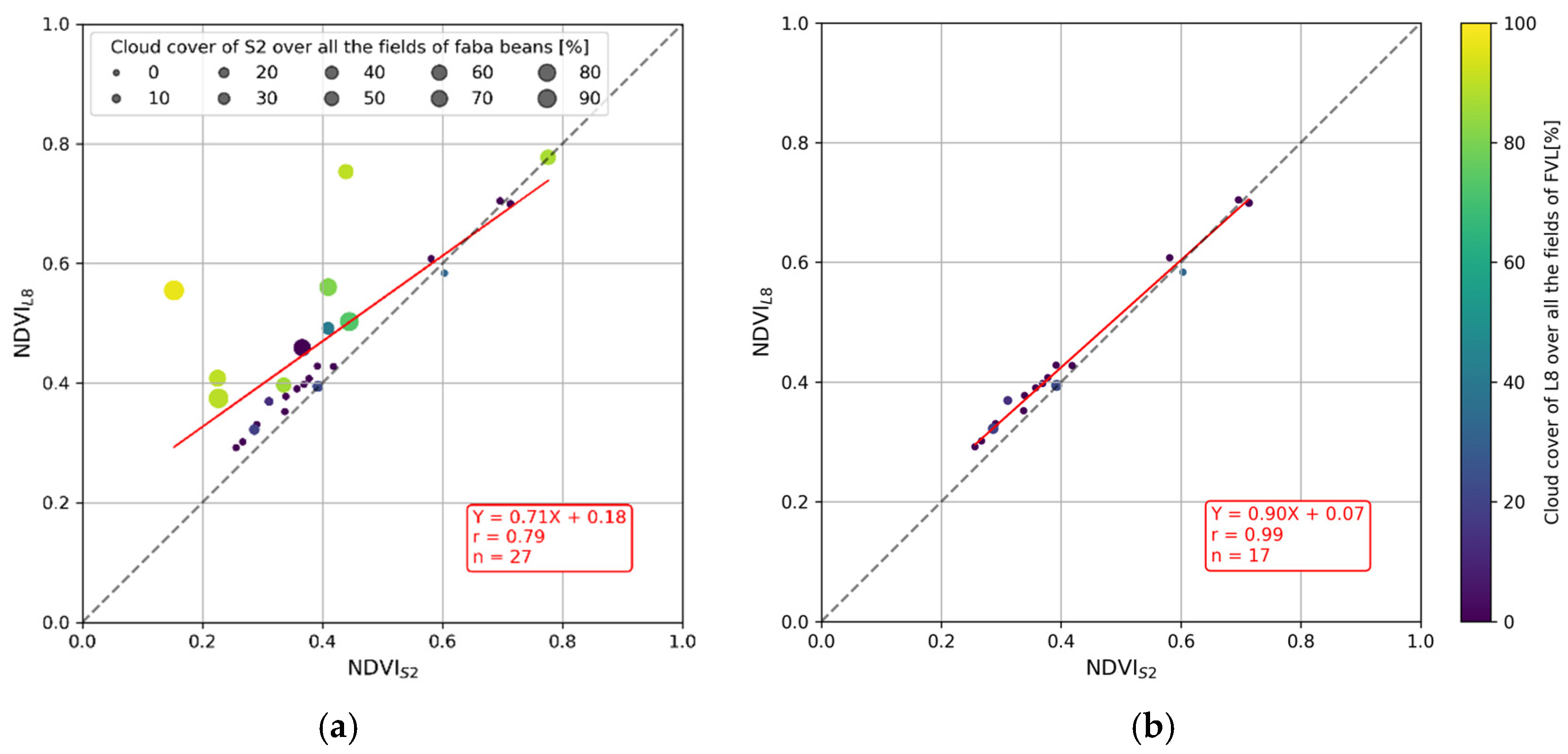The capacity to model the temporal evolution of satellite signals using double logistic (DL) fitting functions is investigated in Section 5.3. 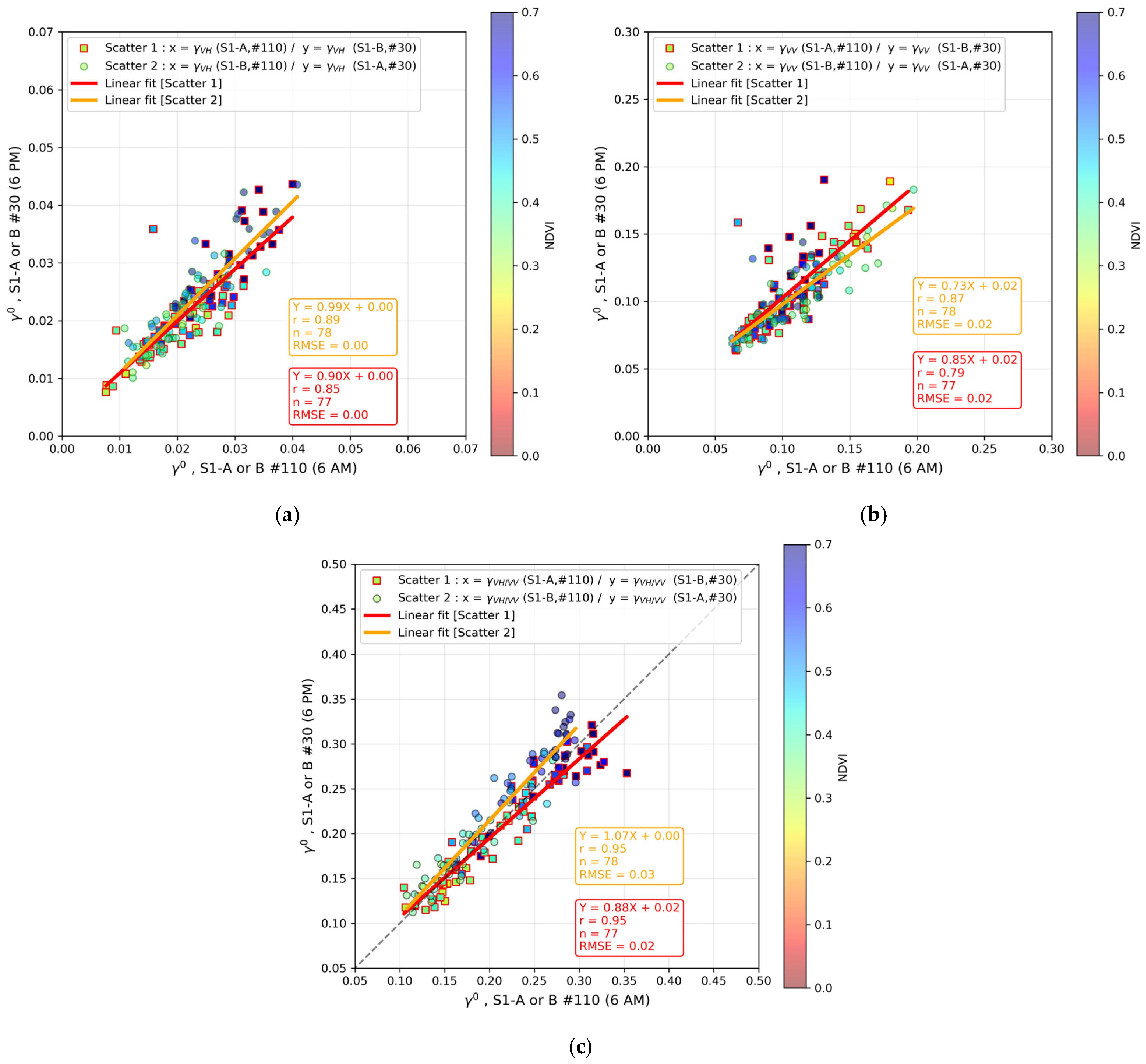The discussion evaluates the impact of mixing optical (Section 6.1) and radar (Section 6.2) data provided by different sensors (Sentinel-2, Landsat-8, and Sentinel-1), considering orbit pass, the time of acquisition (6 a.m. or 6 p.m.), or the difference in spectral bandwidth. Section 6.3 presents an intra-annual analyses of crop development by comparing the field-by-field temporal evolution of satellite signals. In a final sub-section (Section 6.4), the application of these results is extended to the study of faba beans used as an intercrop.

2. Study Site

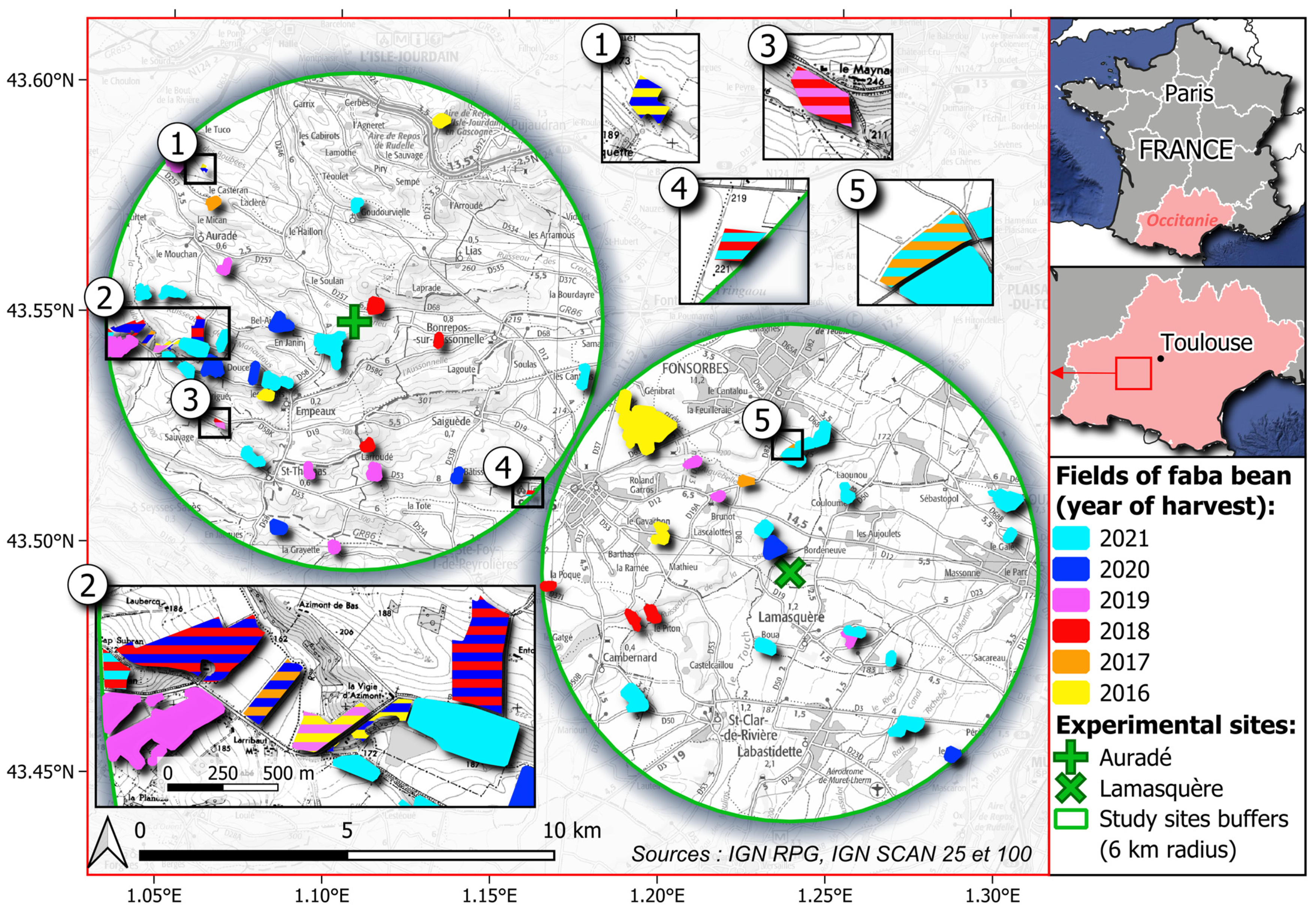
The study site is located in southwestern France in the Occitanie region, which is centered at coordinates 43.52198°N, 1.17032°E (Figure 1). The site is divided into two distinct zones represented by circles with a six-kilometer radius centered on two experimental fields: Auradé and Lamasquère, where weather stations are installed and measure air and soil climatic conditions. The study site is part of a French observatory called Regional Spatial Observatory South-West (RSO SW) and part of the Integrated Carbon Observation System (ICOS) international networks [25,26]. The research activities mainly focused on the monitoring and assessment of natural and anthropogenic determinants of the ecosystem functioning at a regional watershed scale and its landscape. The observatory is also part of the Pyrenees Garonne Regional Workshop Area (ZA PYGAR) and the national Research Infrastructure Critical Zone Observatories: Research and Applications (OZCAR) [27,28]. Moreover, the two experimental sites of Auradé and Lamasquère are part of the JECAM project (Joint Experiment for Crop Assessment and Monitoring—https://jecam.org (accessed on 2 March 2025)). The two zones are partly occupied by urban areas, lakes, and forests (about 10% for the three land use classes). The rest of the area is composed of meadows and annual crops such as maize, sunflowers, wheat, and rapeseed (for the main crops).

Faba beans (a total 78 fields over the surveyed period, Figure 1) are cultivated on a variable number of fields ranging from 4 in 2017 to 30 in 2021. They represent a small part of the total agricultural surface: between 0.16% and 1.56% in 2017 and 2021, respectively. The number of fields is fairly constant in other years: 9 in 2016, 11 in 2018, and 12 in 2019 and 2020. Regardless of the number of faba bean fields, the surface area under cultivation has increased in recent years (from less than 15.4 ha in 2017 to 176.5 ha in 2021). The fields’ delineation and the associated attribute table are provided by the French Services and Payment Agency (ASP). It provides a regulated anonymous version of graphical data from the French Graphical land Plot Register (RPG), associated with the data declared by the French farmers to the state. Different varieties of faba beans can be sown during 2 periods, in spring or in autumn. The French RPG does not make any distinction between sowing periods. The only available information is that the crop is sown before the 31st of May of the current year. Regardless of the sowing date, the crop is harvested in June/July.

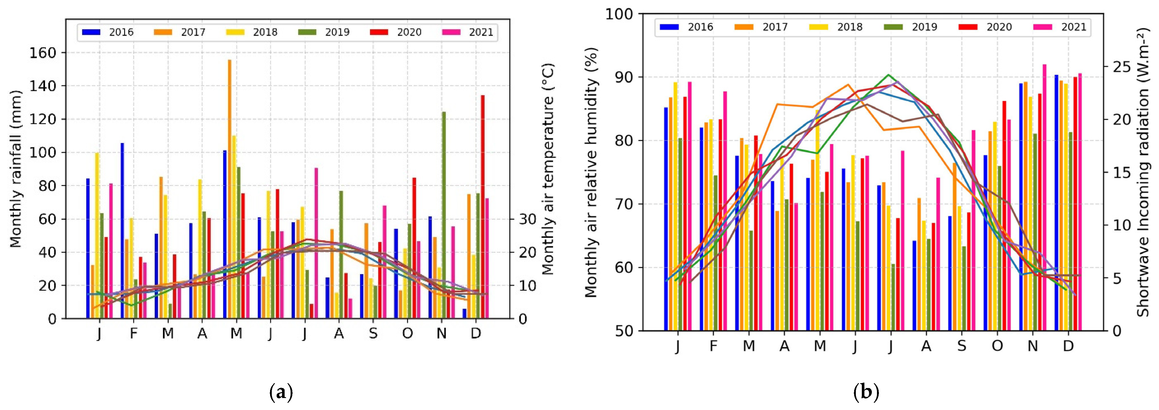
The region is governed by a temperate climate. The Auradé field is subject to natural rainfall (about 600 mm per year on average during the study period), while Lamasquère, submitted to a similar rainfall regime, benefits from an irrigation system (pivot and reel). The mean daily air temperature is ranging from a few degrees in winter to 25 °C in summer. A six-kilometer radius was chosen to maintain proximity to the climate measurement stations while avoiding overlap between the two zones. The slope of the faba bean fields ranges between 0° (horizontal) and 12.48° (2.9° on average for all the fields). The analysis of the rotation of land use shows that most fields change from one year to the next. No field was cultivated with faba beans more than twice during the study period, and only one was cultivated for 2 consecutive years: 2018 and 2019 (zoom number 3 in Figure 1).

3. Dataset

3.1. Ground Data

The annual rainfall in the Auradé field varied between 592 and 827 mm from 2016 to 2021 (Figure 2a). The highest and lowest totals were recorded in 2018 and 2021, respectively. Overall, rainfall shows a well-marked seasonal pattern, with a wetter period in late spring (May), followed by a drier period in summer (July and August) (Figure 2b). Rainfall then increases again in autumn (October and November). There is significant interannual variability, as well as a large monthly variability. In terms of temperature, the seasonal variations are consistent with the typical climate observed in the transition area between ocean and continental climates, with higher temperatures in summer (averaging between 20 °C and 25 °C) and colder temperatures in winter (averaging between 0 °C and 5 °C). Shortwave incoming radiation is recorded in the spectral range from 305 to 2800 nm (by a CNR4 sensor). It also varies significantly from year to year. The distinct seasonal pattern of shortwave radiation observed in the spring of 2017 could be explained by specific climatic conditions. According to the available meteorological data, April 2017 was the driest April (lower precipitation and lower air relative humidity) recorded during the six-year period from 2016 to 2021 (Figure 2a,b). This result suggests a generally drier atmosphere, reducing cloud cover and increasing the transparency of the atmosphere to incoming shortwave radiation. The combination of lower atmospheric humidity, reduced diffuse radiation, and stronger direct solar input likely explains why the peak and shape of the shortwave curve in April 2017 are higher than in other months. In contrast, the lower shortwave radiation values observed from July to September can be attributed to the inverse phenomenon. During this period, increased atmospheric humidity, greater cloud cover, and higher rainfall frequency reduce the amount of incoming shortwave radiation. The climatic data of Lamasquère present similar patterns as those collected in Auradé.

3.2. Satellite Data

3.2.1. Optical Images (Sentinel-2 and Landsat-8)

This study relies on optical data provided by two platforms: Sentinel-2 (A and B) and Landsat-8 (Figure 3). The summary of the bands used, their wavelength intervals, and their spatial resolution are shown in

Table 1. Band names, range of wavelengths, and spatial resolution (R) of Landsat-8 and Sentinel-2 images used.

Landsat-8			Sentinel-2
Band Name	Wavelength (µm)	R (m)	Wavelength (µm)	R (m)
Blue (B2)	0.452–0.512	30	0.459–0.525	10
Green (B3)	0.533–0.590	30	0.542–0.578	10
Red (B4)	0.636–0.673	30	0.650–0.681	10
NIR (B5)	0.851–0.879	30	-	-
NIR (Narrow—B8)	-	-	0.780–0.886	10

. Sentinel-2 is a part of the European Space Agency’s Copernicus program, consisting of two satellites launched in 2015 and 2017. These satellites carry the multi-spectral instrument (MSI) with 13 operational wavelengths and different spatial resolutions at 10, 20, and 60 m [29]. The images can be accessed on the ESA website, where level 2 images with surface reflectance and additional outputs such as aerosol optical thickness and water vapor maps are available. A total of 385 images located at 31TCJ MGRS tile Id. (orbit #51) are downloaded over the period of 2016–2021. Landsat-8 is a satellite launched by NASA and operated by USGS, continuing the Landsat mission of global space image acquisition. It was launched in 2013 and carries the OLI and TIRS sensors [30]. The OLI collects data at nine operational wavelengths and two spatial resolutions of 15 and 30 m. Landsat-8 images can be obtained from the USGS website, with level 2 SR images available for download. A total of 272 images located at #199-30 and #198-30 WRS-2 path/row are downloaded for the study period. The availability of surface reflectance images, along with additional metadata such as cloud probability maps, allows for more accurate and reliable analysis. Cloud/snow masks are derived from processing carried out by the ESA for Sentinel-2 and by the USGS for Landsat. For Sentinel-2, they are based on the official ESA scene classification (SCL) product. For Landsat-8/9, they are based on the NASA pixel quality assurance (QA) band and the C Function of the mask (CFMask) algorithm [31,32].

The satellite data, obtained from reliable sources and with various spatial and temporal resolutions, enable the investigation and monitoring of land surface vegetation dynamics and changes with greater precision over a period of the six studied years (2016–2021). Optical images are used to derive two well-known indexes: NDVI and LAI, with the latter being derived from an algorithm implemented in the SNAP software, version 12.0.0 [33,34].

3.2.2. Radar Images (Sentinel-1A and 1B)

The Sentinel-1 constellation, which is part of the European Space Agency’s Copernicus program, consists of two satellites—Sentinel-1A and Sentinel-1B. (The latter, which broke down in December 2021, has now been replaced by Sentinel-1C.) These satellites’ onboard C-band SAR antennas (center frequency equal to 5.405 GHz) are positioned in the same orbit at an altitude of 693 km, with an orbital phase difference of 180°. The orbit is near-polar and sun-synchronous, with an inclination of 98.18° [35]. The satellites’ antennas operate in four different modes, including the Interferometric Wide swath mode. (The default mode IW is used in this study.) This mode provides spatial resolution of 20 m × 22 m for vertical–vertical and vertical–horizontal polarizations. Orbits #110 and #30 are selected, as they offer complete coverage of the study area, with one acquired at 6 a.m. (descending) and the other at 6 p.m. (ascending) (Figure 3). SAR images can be downloaded at the European Space Agency’s website: https://browser.dataspace.copernicus.eu/ (accessed on 2 March 2025) or selected/processed/visualised/shared/exported from the VisioTerra web platform https://visioterra.org/VtWeb/ (accessed on 2 March 2025). Earth observation data are processed on the fly using POF-ML (Processing On-the-Fly Macro Language) scripts. Sentinel-1 radar products undergo thermal noise removal [36], γ⁰ calibration, and orthorectification. Unlike some previous studies [6,16,37,38,39], this study performs orthorectification using the high-resolution digital terrain model RGE ALTI at a 5 m ground sampling resolution. The model was provided by the French Geographical Institute (IGN) [40]. The resulting processed images have a pixel size of 10 m × 10 m. Over the period of 2016–2021, 361 Sentinel-1A images and 310 Sentinel-1B images were used for the study.

4. Methodology

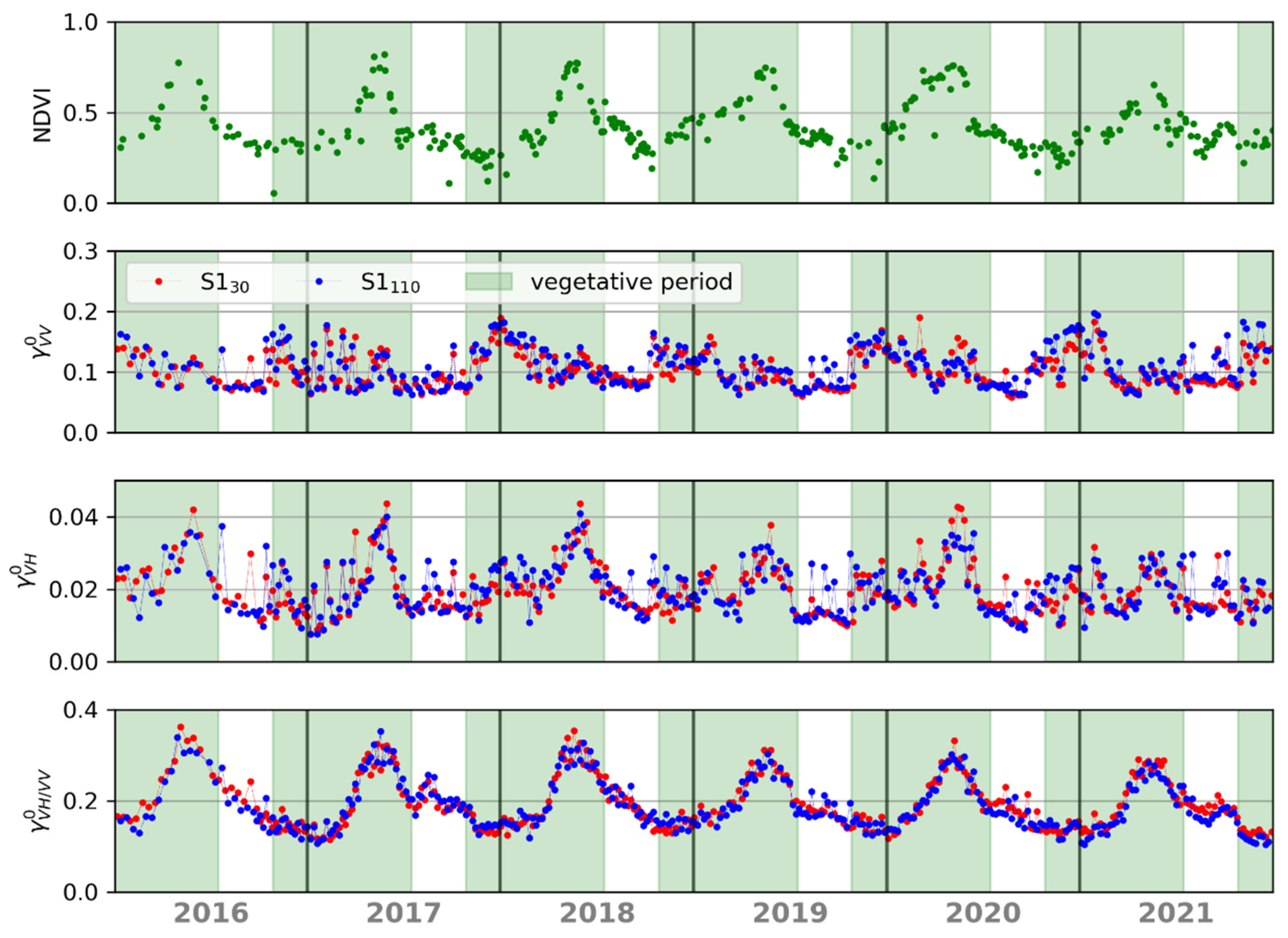
Figure 4 describes the method used in this study. Satellite data are firstly preprocessed as described in Section 3.2. They are then extracted and averaged by field and by year (after applying a 15 m buffer zone to reduce mixing pixels and the field’s border effects) with respect to their shapes. 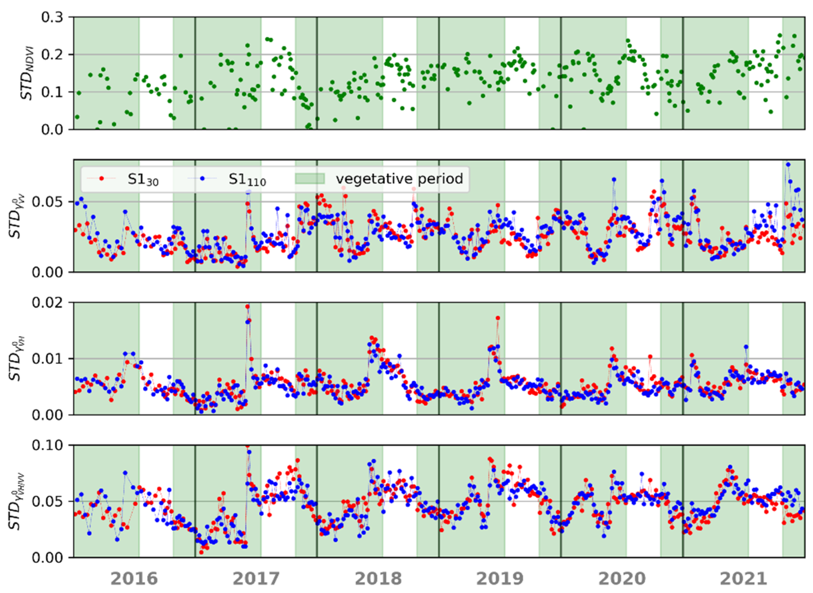Inter- and intra-annual satellite time series are then extracted for the following configurations: NDVI, γ⁰_VV, γ⁰_VH, and γ⁰_VH/VV. The results present an analysis of the time series of the satellite signals. The four configurations are studied through the evolution of their mean and standard deviation over time (Section 5.1). The time series of the vegetation index (VI) that best describe the vegetation (Section 5.2) are then modeled using the DL parametric function (Equation (1)), as already successfully applied on optical and SAR data [39,41,42] (Section 5.3). DL is driven by six metrics that are necessary to describe vegetation phenology.

$$f_{VI}\left(x\right)=In{d}_{min}+\left(In{d}_{max}-In{d}_{min}\right).\left[\left({\displaystyle \frac{1}{1+e^{\left(-G{r}_{Sl}.\left(t-G{r}_{In}\right)\right)}}}\right)-\left({\displaystyle \frac{1}{1+e^{\left(-S{e}_{Sl}.\left(t-S{e}_{In}\right)\right)}}}\right)\right]$$

(1)

where t represents the day of the year. Ind_min and Ind_max are related to the base level and amplitude of the DL, respectively. Gr_in and Se_in determine the date of the inflection points during the growing and senescence periods, respectively. Gr_sl and Se_sl determine the slope during the growing and senescence phases, respectively. The parametric method makes it possible to compare the vegetation monitoring potential of different satellite missions. Its application over several years enables us to characterize, compare, and analyze the dynamics observed, in relation to the agricultural practices and climatic conditions. The quality of each double logistic function is assessed by the values of the coefficient of correlation (r, Equation (2)) and the relative root mean square error (rRMSE, Equation (3)) estimated between fitting curves and satellite data. They are then used to describe vegetation inter-annual development of each crop according to precipitation and temperature information collected in situ (Section 5.4).

$$r={\displaystyle \frac{\mathrm{COV}\left(o,p\right)}{{\sigma }_o{\sigma }_p}}$$

(2)

$$rRMSE [\%]={\displaystyle \frac{RMSE}{〈o〉}}\times 100={\displaystyle \frac{\sqrt{\frac{{\sum }_{i=1}^n{\left(p_i-o_i\right)}^2}{n}}}{〈o〉}}\times 100$$

(3)

where n is the number of observed values, o represents the observed value, p is the predicted value, COV is the covariance, and σ_o and σ_p are the standard deviations of the observed and predicted data, respectively. $〈o〉$ represents the mean of observed values.

5. Results

5.1. Temporal Evolution of Satellite Signal

Figure 5 shows the temporal evolution of the average variations in the optical (NDVI) and radar (γ⁰_VV, γ⁰_VH and γ⁰_VH/VV) signals over the 6 considered years. The fields and their number differ from year to year, as described in Figure 1. The overall growing season of faba beans is represented by vertical green rectangles (between October and July). Changes in amplitude (intensity of the satellite signal) and phase (temporal shift in the signal dynamics) are the consequence of one or more changes in climatic conditions or of the farmer’s field management practices.

The temporal evolution of NDVI and γ⁰_VH/VV is well marked according to the phenological cycle compared to that observed with γ⁰_VV and γ⁰_VH [21,24]. Beyond the marked and recurring seasonal cycle, two specific behaviors can be observed. The first behavior concerns curves where the increase in NDVI or γ⁰_VH/VV begins at the end of the year preceding the harvest. It can be seen in 2018–2019, 2019–2020, and 2020–2021 and is more pronounced for NDVI than for the polarization ratio. The second is when NDVI or γ⁰_VH/VV increase later, such as during spring from about day of year (doy) 100. This behavior is observable in 2015–2016, 2016–2017, and 2017–2018. This difference in crop phenology development can be explained by several factors. The first relates to weather conditions. The growth of faba beans could be favored by a mild and rainy winter, i.e., climatic conditions that are not limiting for the development of the crop [43,44,45]. The second factor is the sowing periods (in autumn or spring) and crop varieties used, agricultural practices which depend on the farmer’s choices. The use of late varieties (sown earlier) could lead to early increases in satellite signals. The lack of information on the varieties used over the studied fields means that this question cannot be answered. It will therefore be examined in greater detail in the Section 6, together with a field-by-field analysis of the satellite time courses.

The γ⁰_VH signal also shows similar trends to the NDVI. However, it varies considerably from one acquisition to another, especially during periods of low vegetation development (when the NDVI is less than 0.4). These variations are due to changes in surface conditions (soil moisture and/or roughness, agricultural work, etc.). This signal is therefore less suitable for monitoring the phenological development of the faba bean crop. The use of γ⁰_VV is even less suitable because it is less correlated with NDVI than the previous one (Table 2).

The temporal evolution of standard deviations of each radar signal is shown in Figure 6. While the NDVI standard deviation provides little information, the radar signals are more interesting. In VV polarization, the standard deviation becomes minimal when the NDVI reaches its maximum each year, that is, when vegetation is fully developed (around doy 140). During this period, the vegetation greatly reduces the contribution of the ground component into the radar signal and masks the effects of changes in soil moisture. The standard deviation becomes significant again during the growth or senescence phase of the crop, which is when plant development is more heterogeneous between fields. The standard deviation of γ⁰_VH increases in the beginning of the senescence phase for 5 years out of the 6 studied. Only the last year does not show any particular increase during the senescence phase, as observed for the standard deviation in VV polarization. The most likely hypothesis is a homogeneity of soil conditions in 2021 (soil moisture/roughness over the 30 fields). The analysis of the standard deviation of the polarization ratio helps us better understand the seeds sown on the studied fields. While the values are high during the intercrop periods, they decrease due to sowing (October) and then increase again at the beginning of the year (around doy 50), followed by a decrease around doy 100 and finally an increase again after the maximum of NDVI until harvest. The two observed peaks reflect two distinct behaviors related to the common cultivation period of fall and spring for faba beans (not visible by plotting the means as presented in Figure 5). This point will be deeper investigated in Section 6.3.

5.2. Are SAR Backscattering Coefficients Good Indicators for Estimating NDVI or LAI?

In this section, the objective is not to reconstruct NDVI time series, like the approaches proposed by [37,38], but to identify (and quantify) the radar indices that best describe the phenological cycle, such as NDVI. Table 2 summarizes the statistical performances obtained from the comparisons of daily interpolated NDVI (or LAI) and SAR backscattering coefficients values using a second-order polynomial regression function. The 6 years (2016–2021) are grouped together in the figures. Overall, performances are uneven, with values ranging from 0.33 to 0.83. The worst results are obtained with VV polarization (r < 0.55 for both NDVI and LAI relationships), where the backscatter coefficients are too strongly affected by variations in soil conditions linked to tillage, roughness, and variations in water content (due to rainfall). Phenology is more visible in cross-polarization (γ⁰_VH), with stronger (but still moderate) correlations for NDVI (r = 0.67 on average) and LAI (r = 0.61 on average) monitoring. These correlations further increase when the polarization ratio (r_NDVI = 0.79 and r_LAI = 0.82) is used. They exceed 0.80 in the best case of orbit 30 (for both LAI and NDVI estimates). This orbit acquires images at a higher angle of incidence (46° on average) than the 110 orbit (42° on average). This geometric property means that the radar signal is more dynamic throughout the phenological cycle and more sensitive to bare soil or fully vegetated periods (Figure 5). The significance of the results (p-value < 0.05, 6 × 10⁻⁵¹ in the worst case) was checked using a Mann–Whitney test, as the distributions of the LAI, NDVI, and radar backscattering coefficient (the γ⁰_VH/VV values on orbits 30 and 110 have been investigated) are not normal (normality assessed using the Shapiro–Wilk test, specially adapted for small datasets). The quality of these results is comparable to that obtained for other legume crops [13,16].

Table 2. Summary of correlation coefficients resulting from the comparison between daily interpolated NDVI (or LAI) and backscattering coefficients (γ⁰_VV, γ⁰_VH and γ⁰_VH/VV) for faba beans. The two orbits are differentiated: 30 or 110. Correlation coefficients are calculated using second-order polynomial regression (y = ax² + bx + c), as illustrated in Figure 7.

	γ0VV (30)	γ0VV (110)	γ0VH (30)	γ0VH (110)	γ0VH/VV (30)	γ0VH/VV (110)
NDVI	0.33	0.38	0.70	0.63	0.81	0.77
LAI	0.43	0.52	0.64	0.57	0.83	0.81

Table 2. Summary of correlation coefficients resulting from the comparison between daily interpolated NDVI (or LAI) and backscattering coefficients (γ⁰_VV, γ⁰_VH and γ⁰_VH/VV) for faba beans. The two orbits are differentiated: 30 or 110. Correlation coefficients are calculated using second-order polynomial regression (y = ax² + bx + c), as illustrated in Figure 7.

	γ0VV (30)	γ0VV (110)	γ0VH (30)	γ0VH (110)	γ0VH/VV (30)	γ0VH/VV (110)
NDVI	0.33	0.38	0.70	0.63	0.81	0.77
LAI	0.43	0.52	0.64	0.57	0.83	0.81

5.3. Modeling Time Series of Satellite Signals with DL Functions to Describe the Phenology

Figure 8 shows an example of the modeling radar (top figure) and optical (bottom subfigure) data from DL fitting functions. Only γ⁰_VH/VV values (in orbits 30 and 110) are shown for the microwave domain because they best represent the vegetation cycle, as demonstrated above. The NDVI modeling results are shown in the lower sub-panel of Figure 8. The blue and orange curves represent the years 2017–2018 and 2020–2021, respectively. Day 1 is the first January of the year before the harvest. All the statistic performances (r, RMSE, and rRMSE) are summarized in

Table 3. Summary of statistical parameters (r, RMSE, and rRMSE) obtained through the modeling of satellite signals (γ⁰_VH/VV and NDVI) using double logistic functions.

Sensor/Orbit		2016	2017	2018	2019	2020	2021	Mean
SAR/30	r	0.94	0.96	0.96	0.97	0.96	0.95	0.96
	RMSE	0.02	0.02	0.02	0.01	0.01	0.02	0.02
	rRMSE (%)	9.96	9.52	8.81	6.99	7.46	8.65	8.57
SAR/110	r	0.92	0.96	0.95	0.96	0.95	0.96	0.95
	RMSE	0.03	0.02	0.02	0.01	0.01	0.01	0.02
	rRMSE (%)	12.10	9.45	9.21	6.86	8.01	8.04	8.95
NDVI/-	r	0.95	0.92	0.94	0.77	0.89	0.85	0.89
	RMSE	0.04	0.07	0.06	0.09	0.07	0.06	0.07
	rRMSE (%)	8.39	16.67	14.65	19.8	15.36	14.84	14.95

. The values of the six parameters of each DL are given in Appendix A.

Figure 8 highlights the good quality of the modeling results for two years (2018 and 2021). The phenological cycle is well reproduced between sowing (in October of the previous year) and harvesting (around July of the current year). Fluctuations in radar signals (slight changes in surface conditions) or NDVI (impact of atmospheric conditions) are perfectly compensated for by the model. Variations in amplitude between years are also well reflected by the models and are consistent between years and sensors. Figure 8 shows that 2018 presents greater development than 2021. This observation is confirmed by the radar data, regardless of the orbit (30 or 110).

The quality of the results is highlighted by the values of the correlation coefficients (Table 3). They range between 0.92 and 0.97 in the microwave domain and between 0.77 and 0.94 for NDVI. The relative errors (rRMSE) are also very low for all the results (<20%). However, they are lower (6.99–12.10%) in the microwave domain (γ⁰_VH/VV) than for NDVI (8.39–19.52%). The good quality of the γ⁰_VH/VV model is explained by the greater number of available radar data, as well as its high stability. Conversely, the impact of clouds/shadows or atmospheric corrections results in small variations in NDVI, reducing modeling performances.

5.4. Inter-Annual Analyses of Crop Development

Figure 9 shows the temporal evolution of satellite signals acquired over the 6 studied years. Only γ⁰_VH/VV values acquired in orbit 30 and NDVI are shown. (The time courses of γ⁰_VH/VV acquired in orbit 110 are similar to those acquired in orbit 30.) Note that data for the winter of 2015 are not available. Consequently, for the period of 2015–2016, double logistics is therefore only optimized from the beginning of 2016. Cumulative rainfall and air temperature are calculated and displayed from the first of January of the year of the harvest to study their impact during spring (main growing season).

Regardless of the satellite signal, reflectance reaches a maximum between doy 375 and doy 395 (from mid-April to the beginning of May of the year of harvest). All the γ⁰_VH/VV DL fits are fairly clustered, and there are no major differences during the winter period. The only difference is the date when the maximum is reached and the amplitude of this maximum. From a temporal point of view, 2020 is the earliest, followed by 2021 and 2017. Conversely, 2018 and 2019 are later. The maximum radar backscatter coefficients reach at the DL peaks are lowest in 2021, 2020, and 2019. On the other hand, the maximum values are higher in 2016, 2017, and 2018. These differences in amplitude and temporal phase are largely related to biomass [10] and provide information on the earliness, production, and possible impact of several abiotic stresses of the crop [37,43,46]. The behavior of the NDVI curves is similar to that of the radar curves for 4 years out of 6 in terms of the amplitudes and phases of the temporal signals. The 2 years that differ significantly are 2019 and 2020. In these cases, the NDVI increases significantly from the end of the previous year, unlike in the other years. This behavior reflects significant plant growth during this period. However, it is not sufficient to be detected using radar data (which are less sensitive to LAI than biomass). In these years, we can expect to see a large number of faba bean fields sown in autumn, unlike in other years where the majority of fields seem to be sown in spring. This point is explored in the Section 6.3.

Information provided by cumulative rainfall and air temperature allows for the refining of previous interpretations. The early growth and highest level of NDVI and γ⁰_VH/VV of faba beans in 2016 are explained, in particular, by a very wet year combined with standard air temperatures [44,45,47]. Conversely, the year 2021 shows sparse leaf development, with an NDVI value not exceeding 0.6. This situation is explained by irregularly distributed rainfall (many plateaus are observed on the cumulative curve) and intense punctual rainfall. In addition, rainfall is deficient from spring onwards, which is when the crop needs it the most. This trend continues until harvest. The cumulative temperatures of 2021, although normal, play a secondary role when rainfall is deficient in the case of a non-irrigated crop. The year 2018 is also notable for recording the highest cumulative rainfall while maintaining average cumulative air temperatures. Although its impact on NDVI is not significantly different from other years such as 2013, 2017, or 2020, the effect on the γ⁰_VH/VV ratio is clearly pronounced. It marks the second highest backscatter response and is comparable to that in 2016, which was the second wettest year. These results suggest that such conditions are indicative of years with greater overall biomass production [10,15,24].

6. Discussions

6.1. Impact of the Satellite Sensor and Cloud/Shadow Detection Capabilities on NDVI Values

The influence of onboard sensors used (OLI and MSI) to derive NDVI is studied because values may vary according to the spectral and radiometric resolution difference in the considered satellites [48]. This phenomenon could explain some of the dispersion of NDVI values over time, such as that between two successive acquisitions performed by Sentinel-2 and Landsat-8. This analysis is complemented by the average cloud cover calculated over all the fields of faba beans. (As a reminder, at the field level, only fields with less than 20% cloud cover are retained.) The good quality of the cloud filters allows most clouds and shadows to be detected, but some pixels may not be detected, resulting in radiometric aberrations unrelated to variations in surface radiometry. The average cloud cover rate gives an indication of the total amount of cloud cover at the scale of the faba bean fields.

Figure 10a compares the NDVI estimated by the satellites Sentinel-2 (A and B) and Landsat-8. Data are extracted on the same acquisition date, all along the vegetation cycle of faba beans. The mean cloud cover, which is estimated over all the fields of faba beans during Landsat-8 acquisition, is represented by a color scale on the right of the figures, whereas the one by Sentinel-2 is represented by the change in the marker size (in the legend panel). Given the variables being compared, which should be identical, the correlation between all points remains low (r = 0.79). This can be explained by the high cloud cover observed in both Landsat-8 (green/yellow dots) and Sentinel-2 (large dots) images. Figure 10a shows that the point cloud variance can be explained by the total cloud cover, despite the prior selection of fields with less than 20% cloud pixels. This result shows that, in some cases, the cloud mask is not precise enough to identify fields whose radiometry is disturbed by clouds and/or their shadows. Setting a threshold of less than 40% to the total cloud cover over faba bean fields significantly reduces the dispersion of NDVI values and mitigates the impact of residual clouds and shadows. This threshold was empirically determined through a series of tests evaluating the trade-off between cloud contamination and data availability. This proved to be the most effective compromise; stricter thresholds resulted in excessive data loss, whereas higher thresholds failed to eliminate radiometric inconsistencies. After applying this filter (<40%), the NDVI values from Sentinel-2 and Landsat-8 became highly consistent, with a correlation coefficient of r = 0.99 (see Figure 10b).

This result shows that the detection of clouds or their shadows needs to be further improved to consolidate cloud masks and measured reflectance (and the associated derived index) values.

However, after applying the cloud cover correction, a small bias remains for low NDVI values. This bias reflects an overestimation of NDVI values from Landsat-8 compared to Sentinel-2. Several factors explain this difference. The first reason is the difference in spatial resolution (10 m and 30 m for Sentinel-2 and Landsat-8, respectively). At the 30 m resolution, field edge effects are more pronounced, despite the cropping of the fields (a negative buffer of 15 m). The radiometric influence of neighboring fields is then also greater. The second reason is the difference in the wavelengths used by the two satellites. Indeed, they measure red and NIR reflectance at different central frequencies and bandwidths. Landsat-8 measures red and NIR reflectance at central wavelengths of 654.5 and 865 nm and at bandwidths of 37 and 28 nm, respectively [30]. Sentinel-2 imagery is acquired at 664.6 (664.9 for Sentinel-2B) and 832.8 (832.9 for Sentinel-2B) nm wavelengths with 31 and 106 nm of bandwidths, respectively [49]. This difference could contribute to a slightly different reflectance measurement, with more or less signal integration in their respective bandwidths (comparable bandwidth in the red but much narrower in the NIR for the MSI sensor onboard S2 satellites). All these combined effects can explain the difference between the two satellites for low NDVI measurements. However, they become negligible as the NDVI increases.

In terms of the DL modeling approach, these effects mainly affect the low NDVI values but not the highest ones. The modeling approach is all the more relevant as it allows these small variations to be smoothed out by approximating all measurements by the double logistic functions (which are not sensitive to one-off variations in signals). This smoothing can be seen clearly in Figure 8 and Figure 9. As a result, the fusion of Sentinel-2 and Landsat-8 data for the phenological monitoring of faba beans using NDVI is fully justified. Moreover, the lower statistical performances of modeling are explained by the difference in wavelength used for the two sensors and by the impact of inaccurate cloud and shadow detection.

6.2. Impact of Orbit and Acquisition Time on Radar Backscatter Coefficients

Figure 11 shows the comparison of γ⁰_VV, γ⁰_VH, or γ⁰_VH/VV backscatters acquired on the same day by Sentinel 1-A and Sentinel 1-B over all the faba bean fields during the entire study period (2016–2021). The acquisitions are quasi-synchronous: some of them are taken at 6 a.m. (shown on the x-axis) and others at 6 p.m. (shown on the y-axis). The color of the dots depends on the daily NDVI value. For each sub-figure (Figure 11a–c), two cases are considered, depending on the order of satellite acquisition. The first case concerns acquisitions made by Sentinel-1A first (6 a.m.) then Sentinel-1B (6 p.m.) (named Scatter 1). The second case represents data where the Sentinel-1B backscatter coefficients are acquired first (named Scatter 2). For each case, linear regression and associated statistical performances (coefficient of correlation and Root Mean Squared Error: RMSE) are calculated. Overall, the backscatter coefficients acquired in the morning and evening from the two different orbits are very similar. Each of the regressions is close to the affine function of y = x, and the coefficient of correlation is superior compared to the value of 0.8 in five out of six cases (r_mean = 0.88). No significant trend is observed as a function of NDVI. These results confirm that it is possible to merge the data acquired by the two Sentinel-1 satellites without affecting the behavior of the radar time series. They also confirm the relevance of merging acquisitions in ascending (evening) and descending (morning) orbits, with no directional and/or temporal effects linked to crop geometry, unlike observations on sunflowers, for example [50]. This point is crucial for improving the temporal resolution of observations in the context of operational crop monitoring. The quality of the DL models is therefore not significantly affected by the merging of SAR data.

6.3. Intra-Annual Analyses of Crop Development

Figure 12 shows the temporal evolution of satellite signals (NDVI and γ⁰_VH/VV in orbit 30) of each field for two different years of cultivation: 2016–2017 (a) and 2019–2020 (b). In 2017, four fields were studied, and twelve were studied in 2020. While the temporal evolution of the average curve in 2017 (Figure 9) indicates a trend towards spring faba bean cultivation, one of the four cultivated fields showed earlier vegetation growth (from December of the previous year), suggesting early sowing in the previous autumn. Among the fields sown in spring, one field (represented by a green curve) has a longer vegetation cycle, although its vegetation starts growing at the same time as the other two (orange and blue curves). This behavior is confirmed by both the γ⁰_VH/VV and optical (NDVI) signals. This phenomenon could be the result of a cultivation practice, the variety of crops sown, or climatic or fertilization constraints that are different from the two other fields [43]. It is important to notice that the use of γ⁰_VH/VV acquired in orbit 110 does not allow us to see an early increase in vegetation development, like the one represented by the red curve in 2017 (because the image is taken at an angle of incidence closer to nadir than in orbit 30). The year 2020 shows a similar trend, with a reverse behavior compared to 2017. Indeed, while the average behavior of the radar and NDVI time courses suggests autumn sowing for all fields, three fields (displayed by dark purple, light purple, and cyan curves) show zero growth in winter and significant growth in spring (a sign of spring sowing).

In all years, harvesting (strongly decreasing of radar and optical signals) takes place between mid-June and mid-July. Only a few fields are harvested later maybe due to disease or late pod filling [43]. The results shown in Figure 12 (confirmed for the other years) highlight the potential use of these two data sources for the temporal and spatial monitoring of the development (and detect any anomalies) of faba beans between different fields within the same year. Although no field-level management data such as sowing or tillage dates are available (particularly because the French RPG does not distinguish between autumn and spring sowing), the satellite data provide a valuable means to overcome this limitation. The contrasting phenological trajectories derived from radar and optical time series make it possible to distinguish sowing periods and growth patterns, even in the absence of explicit ground-based sowing information.

6.4. Faba Beans as an Intercropping Cover Crop: Similarities and Differences with Inter-Annual Phenology Dynamics

Figure 13a shows the phenological cycle observed by satellite data on a faba bean crop used as an intercrop during the period of 2019–2020 on the field of Auradé. In line with previous results, only γ⁰_VH/VV in orbit 30 and NDVI are discussed here (results in orbit 110 are similar). The transposition of the DL modeling approach is entirely appropriate with very high radar and optical performance despite the presence of non-detected clouds or shadows around doy 390 and doy 450 (r_γ0 = 0.93, rRMSE_γ0 = 12.32%, r_NDVI = 0.98, and rRMSE_NDVI = 11.19%). The six model parameters have been reoptimized to adequately describe the satellite data trajectory (

Table 4. Summarize of double logistic regression parameters (Ind_Min, Ind_Max, Gr_Sl, Gr_In, Se_Sl, and Se_In) for γ⁰_VH/VV (orbit 30) and NDVI. SAR parameters are expressed in natural values.

	IND_min	IND_max	Gr_Sl	Gr_In	Se_Sl	Se_In
γ0VH/VV (orbit 30)	0.15	0.40	0.03	423.03	0.18	467.14
NDVI	0.20	0.84	0.05	347.50	3.67	465.66

). The two curves (γ⁰_VH/VV and NDVI) behave in a similar way to those observed in the previous sections (Figure 8, Figure 9 and Figure 12). The main difference is observed on the NDVI during the growing period and at the time of vegetation destruction. NDVI grows quickly and reaches a high value from the late autumn of 2019 and peaks rapidly in 2020. At the destruction time, NDVI decreases sharply, contrary to the results shown in Figure 9 and Figure 12. This can be attributed to the destruction of the vegetation while the faba bean is still green, in preparation for the sowing of a summer crop. As a result, the NDVI drops abruptly (from peak values to levels typically associated with bare soil) within just a few days. In contrast, when the faba bean is cultivated as a cash (annual) crop, the decline in the index during senescence is more gradual and consistent, extending over several weeks prior to harvest. Similarly, radar signals (especially γ⁰_VH/VV) show a sharp decrease in backscatter when the cover crop is destroyed; this is due to a sudden reduction in volume scattering. The biomass from the intercrop remains on the field and is incorporated as green manure to benefit the subsequent cash crop. The sowing and harvesting dates (20 October 2019 and 6 April 2020, respectively) observed in the field and shown in the figure confirm this unusual behavior.

Superimposing the double logistic functions established on the field of Auradé with the averages for the 5 years (2017–2021) previously described (the period of 2015–2016 is not used because it is incomplete) allows us to compare the behavior of satellite signals (amplitudes, growth periods, duration, etc.) between a crop sown in fall, one sown in spring, and one used as an intercrop. Figure 13b shows that the faba bean crop used as an intercrop exhibits atypical behavior compared to the averages of other years. The temporal evolutions of γ⁰_VH/VV and NDVI perfectly describe the faster growth and earlier termination of the vegetative cycle (linked to the destruction of the crop before senescence) of the intercrop. In addition, it can be seen that the radar signal saturates later than the NDVI (doy 450 versus doy 400). Consequently, it allows for the evolution of phenology to be monitored more completely. It will therefore be preferred to the NDVI signal.

7. Conclusions

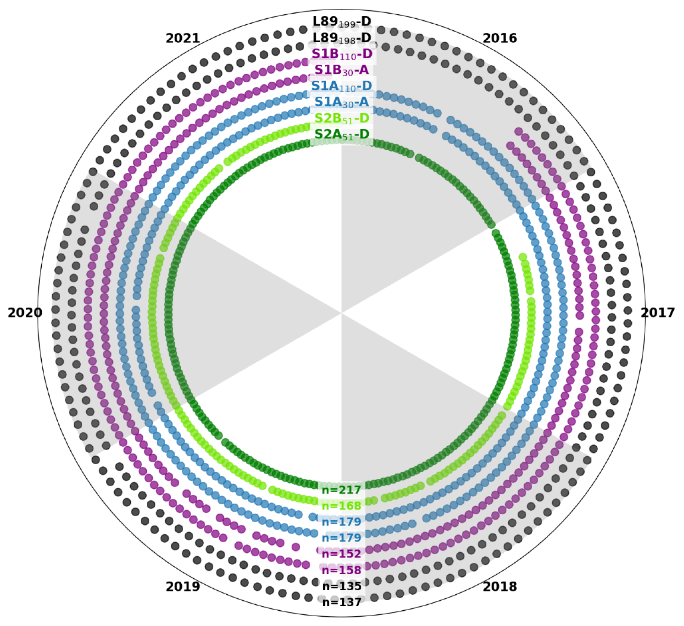
The aim of this article was to explore the capabilities of optical and radar satellite data to monitor the phenology cycle of faba beans. To this end, a dense satellite dataset was collected for 6 years, between the beginning of 2016 and the end of 2021. The size of the satellite image dataset (585 and 671 images processed in the optical and radar domains, respectively), combined with very good knowledge of land use, topography, cloud cover, and meteorology, enabled the quantification of the climatic impact on satellite signals.

The first part of the results shows that the average temporal signatures obtained for faba beans are stable over time. The phenological cycle is perfectly identifiable, and none of the optical (NDVI) or radar (γ⁰_VV, γ⁰_VV, and γ⁰_VH/VV) signals are as saturated as for other legumes like soybeans, unlike many other crops (corn, sunflowers, sorghum, etc.) [6,7,10]. The effects of rainfall and tillage are more visible in the co- and cross-polarization radar signals. The two best indices for monitoring phenology are NDVI and γ⁰_VH/VV. The latter correlates well with NDVI (r = 0.81) and LAI (r = 0.83), especially in orbit 30, where the higher incidence angle provides greater sensitivity to vegetation development. The detailed study at the inter-field scale highlights the disparity of the temporal signatures, which is not visible when studying the average of the temporal signatures. This allows for the identification of agricultural practices, with an emphasis on autumn and spring sowing. Anomalies in plant development are also visible as a function of climatic conditions and/or farming practices. The study of a field of faba beans grown as an intercrop highlighted the similarities and differences between this practice and the use of faba beans as a cash crop sown in autumn or spring. With a sowing similar to that of winter faba beans, plant development is much faster (role of the seed). This is the only case where the NDVI signal saturates early during the growing period. The time of destruction is notable and occurs a few months before the traditional harvest at the end of June. These behaviors are clearly visible on both the NDVI and γ⁰_VH/VV temporal signals.

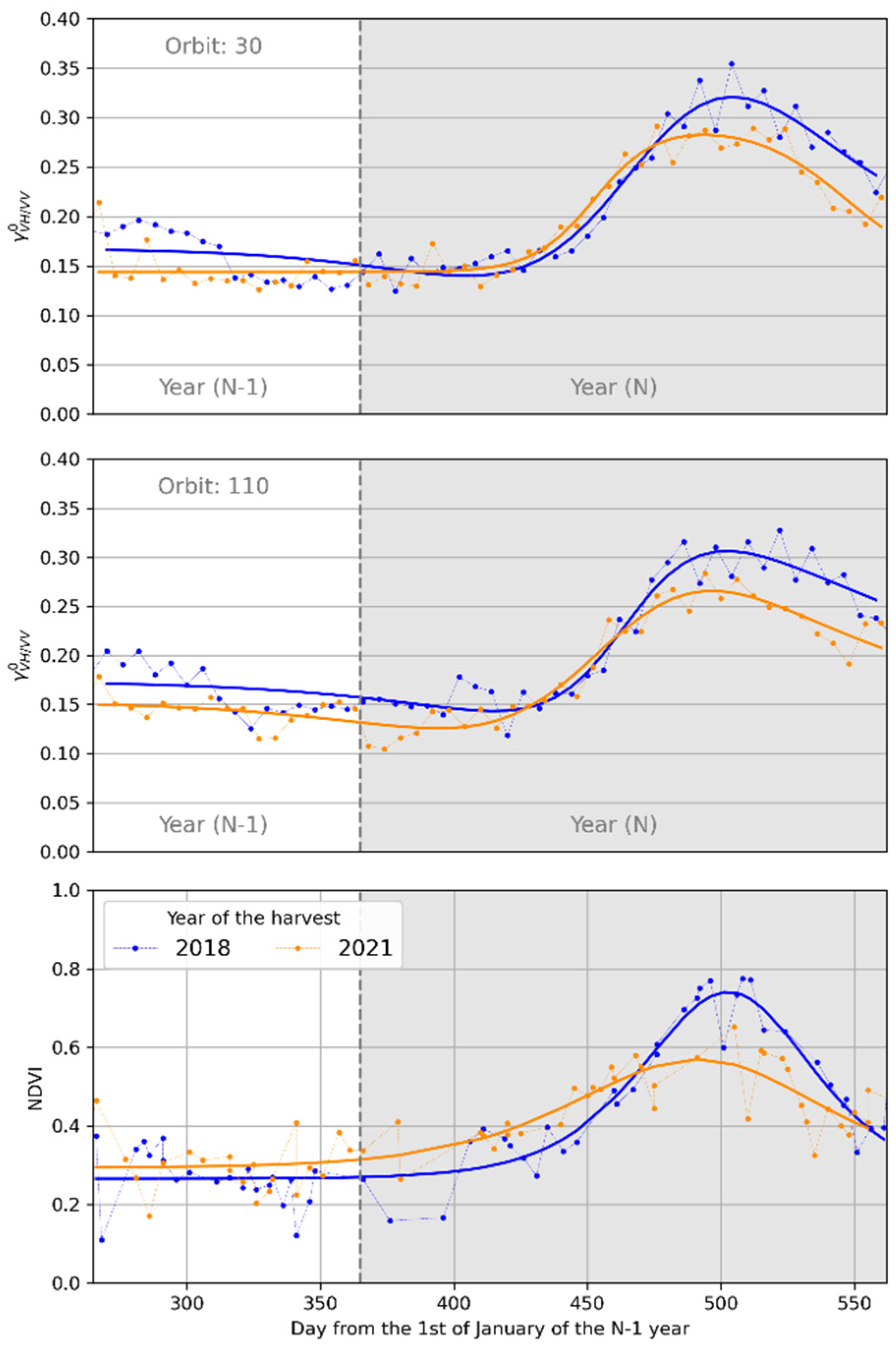
The second part of the results shows that the modeling of temporal signatures using double logistic functions is suitable for this crop. The modeling of the γ⁰_VH/VV signal (for orbits 30 and 110) is excellent, with mean relative errors between years less than 9% and correlation coefficients greater than or equal to 0.95. The quality of the NDVI models is slightly less good (r_mean = 0.89 and rRMSE_mean = 14.91%) but remains sufficient to accurately describe the phenological cycle of the faba bean. This degradation is linked to certain atmospheric conditions: clouds and their shadows, which are not always well detected, interfering with the measurement of NDVI. The inter-annual comparison of the double logistics obtained over the period of 2016–2021 allowed for the definition of average annual envelopes for the phenology trajectory of faba beans. These envelopes can serve as a reference in the literature for the annual study of faba bean phenology in the coming years as part of an operational approach to real-time monitoring. Moreover, the intra-annual results demonstrate how satellite time series can be used to refine and enhance phenological monitoring (between autumn versus spring crop sowing), especially in contexts where administrative data are incomplete or imprecise (like those provided by the French RPG).

The results of this study demonstrate the usefulness of multiwavelength and multi-remotely sensed observations, which can be used together or separately for monitoring and modelling the temporal evolution of faba bean phenology. In light of this study, it would be interesting to test this method over other land uses. It would also be interesting to apply the method on other SAR data, such as those offered by TerraSAR-X (X-band), Cosmos-Skymed (X-band), or ALOS-2 (L-band) and NISAR (S and L bands) and Biomass (P-band) in the near future. Future work could also integrate scattering models to further strengthen the interpretation of the temporal evolution of the SAR signal.

References

1. Jensen, E.S.; Peoples, M.B.; Hauggaard-Nielsen, H. Faba Bean in Cropping Systems. Field Crops Res. 2010, 115, 203–216. [Google Scholar] [CrossRef]
2. Dhull, S.B.; Kidwai, M.K.; Noor, R.; Chawla, P.; Rose, P.K. A Review of Nutritional Profile and Processing of Faba Bean. Vicia Faba 2021, 4, e129. [Google Scholar]
3. Stagnari, F.; Maggio, A.; Galieni, A.; Pisante, M. Multiple Benefits of Legumes for Agriculture Sustainability: An Overview. Chem. Biol. Technol. Agric. 2017, 4, 2. [Google Scholar] [CrossRef]
4. Jensen, E.S.; Peoples, M.B.; Boddey, R.M.; Gresshoff, P.M.; Hauggaard-Nielsen, H.; JR Alves, B.; Morrison, M.J. Legumes for Mitigation of Climate Change and the Provision of Feedstock for Biofuels and Biorefineries. A Review. Agron. Sustain. Dev. 2012, 32, 329–364. [Google Scholar] [CrossRef]
5. Bonnet, C.; Gaudio, N.; Alletto, L.; Raffaillac, D.; Bergez, J.-E.; Debaeke, P.; Gavaland, A.; Willaume, M.; Bedoussac, L.; Justes, E. Design and Multicriteria Assessment of Low-Input Cropping Systems Based on Plant Diversification in Southwestern France. Agron. Sustain. Dev. 2021, 41, 65. [Google Scholar] [CrossRef]
6. Veloso, A.; Mermoz, S.; Bouvet, A.; Le Toan, T.; Planells, M.; Dejoux, J.-F.; Ceschia, E. Understanding the Temporal Behavior of Crops Using Sentinel-1 and Sentinel-2-like Data for Agricultural Applications. Remote Sens. Environ. 2017, 199, 415–426. [Google Scholar] [CrossRef]
7. Baup, F.; Ameline, M.; Fieuzal, R.; Frappart, F.; Corgne, S.; Berthoumieu, J.-F. Temporal Evolution of Corn Mass Production Based on Agro-Meteorological Modelling Controlled by Satellite Optical and SAR Images. Remote Sens. 2019, 11, 1978. [Google Scholar] [CrossRef]
8. Hu, X.; Li, L.; Huang, J.; Zeng, Y.; Zhang, S.; Su, Y.; Hong, Y.; Hong, Z. Radar Vegetation Indices for Monitoring Surface Vegetation: Developments, Challenges, and Trends. Sci. Total Environ. 2024, 945, 173974. [Google Scholar] [CrossRef]
9. Ameline, M.; Fieuzal, R.; Betbeder, J.; Berthoumieu, J.; Baup, F. Estimation of Corn Yield by Assimilating SAR and Optical Time Series Into a Simplified Agro-Meteorological Model: From Diagnostic to Forecast. IEEE J. Sel. Top. Appl. Earth Obs. Remote Sens. 2018, 11, 4747–4760. [Google Scholar] [CrossRef]
10. Betbeder, J.; Fieuzal, R.; Baup, F. Assimilation of LAI and Dry Biomass Data from Optical and SAR Images Into an Agro-Meteorological Model to Estimate Soybean Yield. IEEE J. Sel. Top. Appl. Earth Obs. Remote Sens. 2016, 9, 2540–2553. [Google Scholar] [CrossRef]
11. Claverie, M.; Demarez, V.; Duchemin, B.; Hagolle, O.; Ducrot, D.; Marais-Sicre, C.; Dejoux, J.-F.; Huc, M.; Keravec, P.; Béziat, P.; et al. Maize and Sunflower Biomass Estimation in Southwest France Using High Spatial and Temporal Resolution Remote Sensing Data. Remote Sens. Environ. 2012, 124, 844–857. [Google Scholar] [CrossRef]
12. Fieuzal, R.; Baup, F.; Marais-Sicre, C. Monitoring Wheat and Rapeseed by Using Synchronous Optical and Radar Satellite Data—From Temporal Signatures to Crop Parameters Estimation. Adv. Remote Sens. 2013, 2, 162–180. [Google Scholar] [CrossRef]
13. Hosseini, M.; McNairn, H.; Merzouki, A.; Pacheco, A. Estimation of Leaf Area Index (LAI) in Corn and Soybeans Using Multi-Polarization C- and L-Band Radar Data. Remote Sens. Environ. 2015, 170, 77–89. [Google Scholar] [CrossRef]
14. McNairn, H.; Kross, A.; Lapen, D.; Caves, R.; Shang, J. Early Season Monitoring of Corn and Soybeans with TerraSAR-X and RADARSAT-2. Int. J. Appl. Earth Obs. Geoinform. 2014, 28, 252–259. [Google Scholar] [CrossRef]
15. Kross, A.; McNairn, H.; Lapen, D.; Sunohara, M.; Champagne, C. Assessment of RapidEye Vegetation Indices for Estimation of Leaf Area Index and Biomass in Corn and Soybean Crops. Int. J. Appl. Earth Obs. Geoinform. 2015, 34, 235–248. [Google Scholar] [CrossRef]
16. Mercier, A.; Betbeder, J.; Baudry, J.; Le Roux, V.; Spicher, F.; Lacoux, J.; Roger, D.; Hubert-Moy, L. Evaluation of Sentinel-1 & 2 Time Series for Predicting Wheat and Rapeseed Phenological Stages. ISPRS J. Photogramm. Remote Sens. 2020, 163, 231–256. [Google Scholar] [CrossRef]
17. Steele-Dunne, S.C.; McNairn, H.; Monsivais-Huertero, A.; Judge, J.; Liu, P.-W.; Papathanassiou, K. Radar Remote Sensing of Agricultural Canopies: A Review. IEEE J. Sel. Top. Appl. Earth Obs. Remote Sens. 2017, 10, 2249–2273. [Google Scholar] [CrossRef]
18. Wiseman, G.; McNairn, H.; Homayouni, S.; Shang, J. RADARSAT-2 Polarimetric SAR Response to Crop Biomass for Agricultural Production Monitoring. IEEE J. Sel. Top. Appl. Earth Obs. Remote Sens. 2014, 7, 4461–4471. [Google Scholar] [CrossRef]
19. Gorrab, A.; Ameline, M.; Albergel, C.; Baup, F. Use of Sentinel-1 Multi-Configuration and Multi-Temporal Series for Monitoring Parameters of Winter Wheat. Remote Sens. 2021, 13, 553. [Google Scholar] [CrossRef]
20. Shen, Y.; Liu, X. Phenological Changes of Corn and Soybeans over U.S. by Bayesian Change-Point Model. Sustainability 2015, 7, 6781–6803. [Google Scholar] [CrossRef]
21. Mohammadi, S.; Uhlen, A.K.; Lillemo, M.; Ergon, Å.; Shafiee, S. Enhancing Phenotyping Efficiency in Faba Bean Breeding: Integrating UAV Imaging and Machine Learning. Precis. Agric. 2024, 25, 1502–1528. [Google Scholar] [CrossRef]
22. Ji, Y.; Liu, R.; Xiao, Y.; Cui, Y.; Chen, Z.; Zong, X.; Yang, T. Faba Bean Above-Ground Biomass and Bean Yield Estimation Based on Consumer-Grade Unmanned Aerial Vehicle RGB Images and Ensemble Learning. Precis. Agric. 2023, 24, 1439–1460. [Google Scholar] [CrossRef]
23. Ji, Y.; Liu, Z.; Liu, R.; Wang, Z.; Zong, X.; Yang, T. High-Throughput Phenotypic Traits Estimation of Faba Bean Based on Machine Learning and Drone-Based Multimodal Data. Comput. Electron. Agric. 2024, 227, 109584. [Google Scholar] [CrossRef]
24. Ji, Y.; Chen, Z.; Cheng, Q.; Liu, R.; Li, M.; Yan, X.; Li, G.; Wang, D.; Fu, L.; Ma, Y.; et al. Estimation of Plant Height and Yield Based on UAV Imagery in Faba Bean (Vicia faba L.). Plant Methods 2022, 18, 26. [Google Scholar] [CrossRef]
25. Dejoux, J.-F.; Dedieu, G.; Hagolle, O.; Ducrot, D.; Menaut, J.-C.; Ceschia, E.; Baup, F.; Demarez, V.; Marais-Sicre, C.; Kadiri, M.; et al. Kalideos OSR MiPy: Un Observatoire Pour La Recherche et La Démonstration Des Applications de La Télédétection à La Gestion Des Territoires. Rev. Fr. Photogramm. Télédétec. 2012, 17–30. [Google Scholar] [CrossRef]
26. Franz, D.; Acosta, M.; Altimir, N.; Arriga, N.; Arrouays, D.; Aubinet, M.; Aurela, M.; Ayres, E.; López-Ballesteros, A.; Barbaste, M. Towards Long-Term Standardised Carbon and Greenhouse Gas Observations for Monitoring Europe’s Terrestrial Ecosystems: A Review. Int. Agrophys. 2018, 32, 439–455. [Google Scholar] [CrossRef]
27. Ouin, A.; Andrieu, É.; Vialatte, A.; Balent, G.; Barbaro, L.; Blanco, J.; Ceschia, E.; Clement, F.; Fauvel, M.; Gallai, N. Building a Shared Vision of the Future for Multifunctional Agricultural Landscapes. Lessons from a Long Term Socio-Ecological Research Site in South-Western France. In Advances in Ecological Research; Elsevier: Amsterdam, The Netherlands, 2021; Volume 65, pp. 57–106. ISBN 0065-2504. [Google Scholar]
28. Gaillardet, J.; Braud, I.; Hankard, F.; Anquetin, S.; Bour, O.; Dorfliger, N.; De Dreuzy, J.-R.; Galle, S.; Galy, C.; Gogo, S. OZCAR: The French Network of Critical Zone Observatories. Vadose Zone J. 2018, 17, 1–24. [Google Scholar] [CrossRef]
29. Drusch, M.; Del Bello, U.; Carlier, S.; Colin, O.; Fernandez, V.; Gascon, F.; Hoersch, B.; Isola, C.; Laberinti, P.; Martimort, P. Sentinel-2: ESA’s Optical High-Resolution Mission for GMES Operational Services. Remote Sens. Environ. 2012, 120, 25–36. [Google Scholar] [CrossRef]
30. Irons, J.R.; Dwyer, J.L.; Barsi, J.A. The next Landsat Satellite: The Landsat Data Continuity Mission. Remote Sens. Environ. 2012, 122, 11–21. [Google Scholar] [CrossRef]
31. Zhu, Z.; Wang, S.; Woodcock, C.E. Improvement and Expansion of the Fmask Algorithm: Cloud, Cloud Shadow, and Snow Detection for Landsats 4–7, 8, and Sentinel 2 Images. Remote Sens. Environ. 2015, 159, 269–277. [Google Scholar] [CrossRef]
32. Foga, S.; Scaramuzza, P.L.; Guo, S.; Zhu, Z.; Dilley, R.D.; Beckmann, T.; Schmidt, G.L.; Dwyer, J.L.; Joseph Hughes, M.; Laue, B. Cloud Detection Algorithm Comparison and Validation for Operational Landsat Data Products. Remote Sens. Environ. 2017, 194, 379–390. [Google Scholar] [CrossRef]
33. Weiss, M.; Baret, F.; Jay, S. S2ToolBox Level 2 Products: LAI, FAPAR, FCOVER. Available online: https://step.esa.int/docs/extra/ATBD_S2ToolBox_L2B_V1.1.pdf (accessed on 2 March 2025).
34. Tucker, C.J. Red and Photographic Infrared Linear Combinations for Monitoring Vegetation. Remote Sens. Environ. 1979, 8, 127–150. [Google Scholar] [CrossRef]
35. Torres, R.; Snoeij, P.; Geudtner, D.; Bibby, D.; Davidson, M.; Attema, E.; Potin, P.; Rommen, B.; Floury, N.; Brown, M.; et al. GMES Sentinel-1 Mission. Remote Sens. Environ. 2012, 120, 9–24. [Google Scholar] [CrossRef]
36. Piantanida, R.; Miranda, N.; Hajduch, G. Thermal Denoising of Products Generated by the S-1 IPF 2017. Available online: https://sentinels.copernicus.eu/documents/247904/2142675/Thermal-Denoising-of-Products-Generated-by-Sentinel-1-IPF.pdf (accessed on 2 March 2025).
37. Ayari, E.; Kassouk, Z.; Lili-Chabaane, Z.; Ouaadi, N.; Baghdadi, N.; Zribi, M. NDVI Estimation Using Sentinel-1 Data over Wheat Fields in a Semiarid Mediterranean Region. GISci. Remote Sens. 2024, 61, 2357878. [Google Scholar] [CrossRef]
38. Chen, D.; Hu, H.; Liao, C.; Ye, J.; Bao, W.; Mo, J.; Wu, Y.; Dong, T.; Fan, H.; Pei, J. Crop NDVI Time Series Construction by Fusing Sentinel-1, Sentinel-2, and Environmental Data with an Ensemble-Based Framework. Comput. Electron. Agric. 2023, 215, 108388. [Google Scholar] [CrossRef]
39. Vavlas, N.-C.; Waine, T.W.; Meersmans, J.; Burgess, P.J.; Fontanelli, G.; Richter, G.M. Deriving Wheat Crop Productivity Indicators Using Sentinel-1 Time Series. Remote Sens. 2020, 12, 2385. [Google Scholar] [CrossRef]
40. Ygorra, B.; Frappart, F.; Wigneron, J.P.; Moisy, C.; Catry, T.; Baup, F.; Hamunyela, E.; Riazanoff, S. Monitoring Loss of Tropical Forest Cover from Sentinel-1 Time-Series: A CuSum-Based Approach. Int. J. Appl. Earth Obs. Geoinform. 2021, 103, 102532. [Google Scholar] [CrossRef]
41. Soudani, K.; Delpierre, N.; Berveiller, D.; Hmimina, G.; Vincent, G.; Morfin, A.; Dufrêne, É. Potential of C-Band Synthetic Aperture Radar Sentinel-1 Time-Series for the Monitoring of Phenological Cycles in a Deciduous Forest. Int. J. Appl. Earth Obs. Geoinform. 2021, 104, 102505. [Google Scholar] [CrossRef]
42. Sun, C.; Li, J.; Cao, L.; Liu, Y.; Jin, S.; Zhao, B. Evaluation of Vegetation Index-Based Curve Fitting Models for Accurate Classification of Salt Marsh Vegetation Using Sentinel-2 Time-Series. Sensors 2020, 20, 5551. [Google Scholar] [CrossRef]
43. Sufar, E.K.; Hasanaliyeva, G.; Wang, J.; Leifert, H.; Shotton, P.; Bilsborrow, P.; Rempelos, L.; Volakakis, N.; Leifert, C. Effect of Climate, Crop Protection, and Fertilization on Disease Severity, Growth, and Grain Yield Parameters of Faba Beans (Vicia faba L.) in Northern Britain: Results from the Long-Term NFSC Trials. Agronomy 2024, 14, 422. [Google Scholar] [CrossRef]
44. Pszczółkowska, A.; Okorski, A.; Fordoński, G.; Kotecki, A.; Kozak, M.; Dzienis, G. Effect of Weather Conditions on Yield and Health Status of Faba Bean Seeds in Poland. Agronomy 2019, 10, 48. [Google Scholar] [CrossRef]
45. Manning, B.K.; Trethowan, R.; Adhikari, K.N. Impact of Temperature on Podding in Faba Bean (Vicia faba). Agronomy 2024, 14, 2309. [Google Scholar] [CrossRef]
46. Alza, J.O.; Gutiérrez, N.; Cabezas, J.M.; Torres, A.M.; Lorite, I.J. Interactive Effects of Atmospheric CO2 Concentration and Water Stress on the Phenology and Physiology of Faba Bean (Vicia faba L.). Environ. Exp. Bot. 2024, 218, 105571. [Google Scholar] [CrossRef]
47. Bogale, G.A.; Mengesha, M.; Hadgu, G. Characterization of Local Climate and Its Impact on Faba Bean (Vicia faba L.) Yield in Central Ethiopia. Adv. Meteorol. 2022, 2022, 759596. [Google Scholar] [CrossRef]
48. Mandanici, E.; Bitelli, G. Preliminary Comparison of Sentinel-2 and Landsat 8 Imagery for a Combined Use. Remote Sens. 2016, 8, 1014. [Google Scholar] [CrossRef]
49. Tao, Y.; Xiong, S.; Song, R.; Muller, J.-P. Towards Streamlined Single-Image Super-Resolution: Demonstration with 10 m Sentinel-2 Colour and 10–60 m Multi-Spectral VNIR and SWIR Bands. Remote Sens. 2021, 13, 2614. [Google Scholar] [CrossRef]
50. Qadir, A.; Skakun, S.; Eun, J.; Prashnani, M.; Shumilo, L. Sentinel-1 Time Series Data for Sunflower (Helianthus annuus) Phenology Monitoring. Remote Sens. Environ. 2023, 295, 113689. [Google Scholar] [CrossRef]
Figure 1. Location of the study site in southwestern France, together with the network of the studied fields of faba beans (78 during the 2016–2021 period) superimposed on a Scan100 and Scan25 plan provided by the IGN (French National Geographic Institute). The fields’ color depends on the year of harvest: yellow for 2016, orange for 2017, red for 2018, pink for 2019, blue for 2020, and light blue for 2021. Fields with several colors have been cultivated with faba beans over several years. Five zoom windows (marked from 1 to 5) give a better view of the small fields.
Remotesensing 17 01933 g001
Figure 2. Multi-year ombrothermic diagram (air temperature and cumulative monthly rainfalls collected at 2 m in high) (a) and shortwave incoming radiation and monthly air relative humidity (b) of the sites of Auradé.
Remotesensing 17 01933 g002
Figure 3. Chronogram of satellite acquisitions from 2016 to 2021. Sentinel-1A and 1B acquisitions are separated according to their orbit number (110 or 30) and direction (ascending: A or descending: D) (S1A110-D, S1A30-A, S1B110-D, and S1B30-A) as Landsat-8 (L8199-D and L8198-D) and Sentinel-2 data (S2A051-D and S2B051-D).
Remotesensing 17 01933 g003
Figure 4. Methodological diagram of the steps involved in the paper: from field data acquisition and processing to the sections presented in the Section 5 and Section 6.
Remotesensing 17 01933 g004
Figure 5. Temporal evolution of satellite signals (NDVI, γ0VV, γ0VH, and γ0VH/VV) of faba beans between 2016 and 2021. Satellite signals are averaged over all the studied fields per year (from 4 to 30 fields, Figure 2) and are displayed according to their orbit number: 30 or 110 in the case of radar acquisitions.
Remotesensing 17 01933 g005
Figure 6. Temporal evolution of the standard deviation of satellite signals (NDVI, γ0VV, γ0VH, and γ0VH/VV) of faba beans between 2016 and 2021. The orbit numbers 30 and 110 are mentioned in the case of radar data.
Remotesensing 17 01933 g006
Figure 7. Relationship between the best radar satellite signals (γ0VH/VV (30)), NDVI (a), and LAI (b). NDVI and LAI values are derived from Sentinel-2 and Landsat-8 images and are daily interpolated.
Remotesensing 17 01933 g007
Figure 8. Example of modeling radar (top and middle) and optical (bottom) data from DL fitting functions. Satellite measurements are represented by dots. The blue and orange curves represent the DL of the years 2018 and 2021, respectively. Day 1 is the first January of the previous year (year of potential sowing).
Remotesensing 17 01933 g008
Figure 9. Superimposing satellite observations (γ0VH/VV (30) or NDVI) and modeling based on double logistic functions for the 6 studied years. Satellite measurements are represented by dots (one color for each year). The same color is kept for DL fitting functions. Day 1 is the first January of the previous year (year of potential sowing). The temporal accumulation of air temperature and rainfall is displayed from the first of January of the year of harvest.
Remotesensing 17 01933 g009
Figure 10. Comparison of NDVI estimated the same day by Sentinel-2 and Landsat-8 according to the average cloud cover estimated over all the fields of faba beans while considering the mean cloud cover level (a) or only the mean cloud cover inferior or equal to 40% for all fields (b). The legends for Sentinel-2 and Landsat-8 cloud cover apply to the 2 sub-figures.
Remotesensing 17 01933 g010
Figure 11. Comparison of backscattering coefficients acquired by Sentinel-1A and B. The acquisitions are quasi-synchronous: the first is taken at 6 a.m. on orbit #110 (represented on the x-axis) and the second at 6 p.m. on orbit #30 (represented on the y-axis). The color of the dots depends on the daily interpolated NDVI value. Three cases are presented here: (a) γ0VH, (b) γ0VV, and (c) γ0VH/VV.
Remotesensing 17 01933 g011
Figure 12. Temporal evolution of some satellite signals (NDVI and γ0VH/VV in orbit 30) of each field for two different years: 2016–2017 (a) and 2019–2020 (b). In 2017, four fields were studied, and twelve were studied in 2020. Each curve color represents a different field. Field identifiers are not shown to keep the figure simple.
Remotesensing 17 01933 g012
Figure 13. Temporal evolution of measured (black dots) and modeled (blue and green double logistic fitting functions for γ0VH/VV and NDVI, respectively) γ0VH/VV and NDVI for the field of Auradé (where the faba bean is used as an intercrop in 2019–2020) (a). Superposition of the DL functions established between 2017 and 2021 with those obtained on the Auradé field. The transparent green area represents the interval between the double logistic over the period of 2017–2021 (b). Sowing and destruction dates given by the farmer are noted by vertical dotted black lines on 20 October 2019 and 7 April 2020, respectively.
Remotesensing 17 01933 g013