
Street-Scale Urban Air Temperatures Predicted by Simple High-Resolution Cover- and Shade-Weighted Surface Temperature Mosaics in a Variety of Residential Neighborhoods


Abstract
1. Introduction
2. Methods
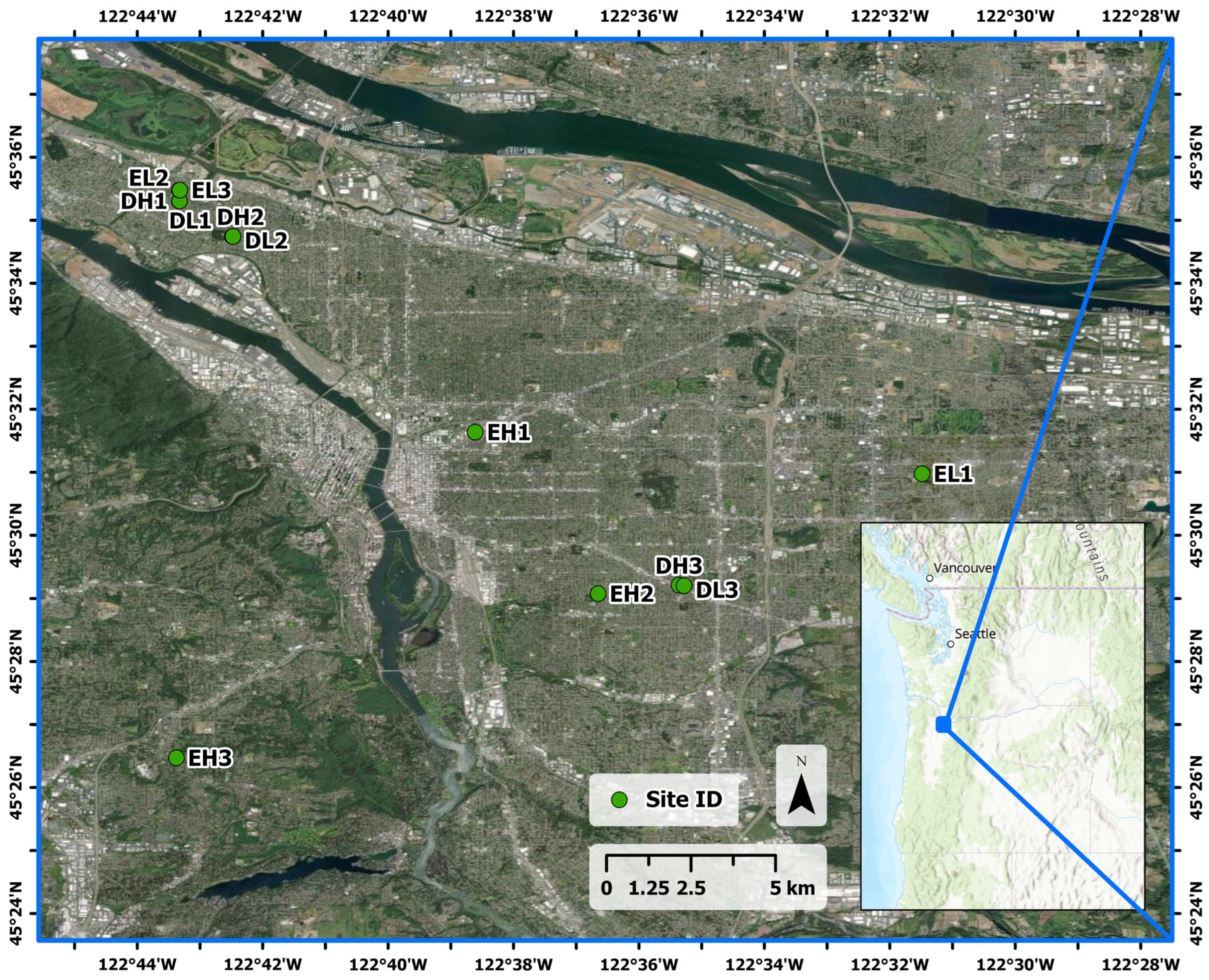
2.1. Field Sites
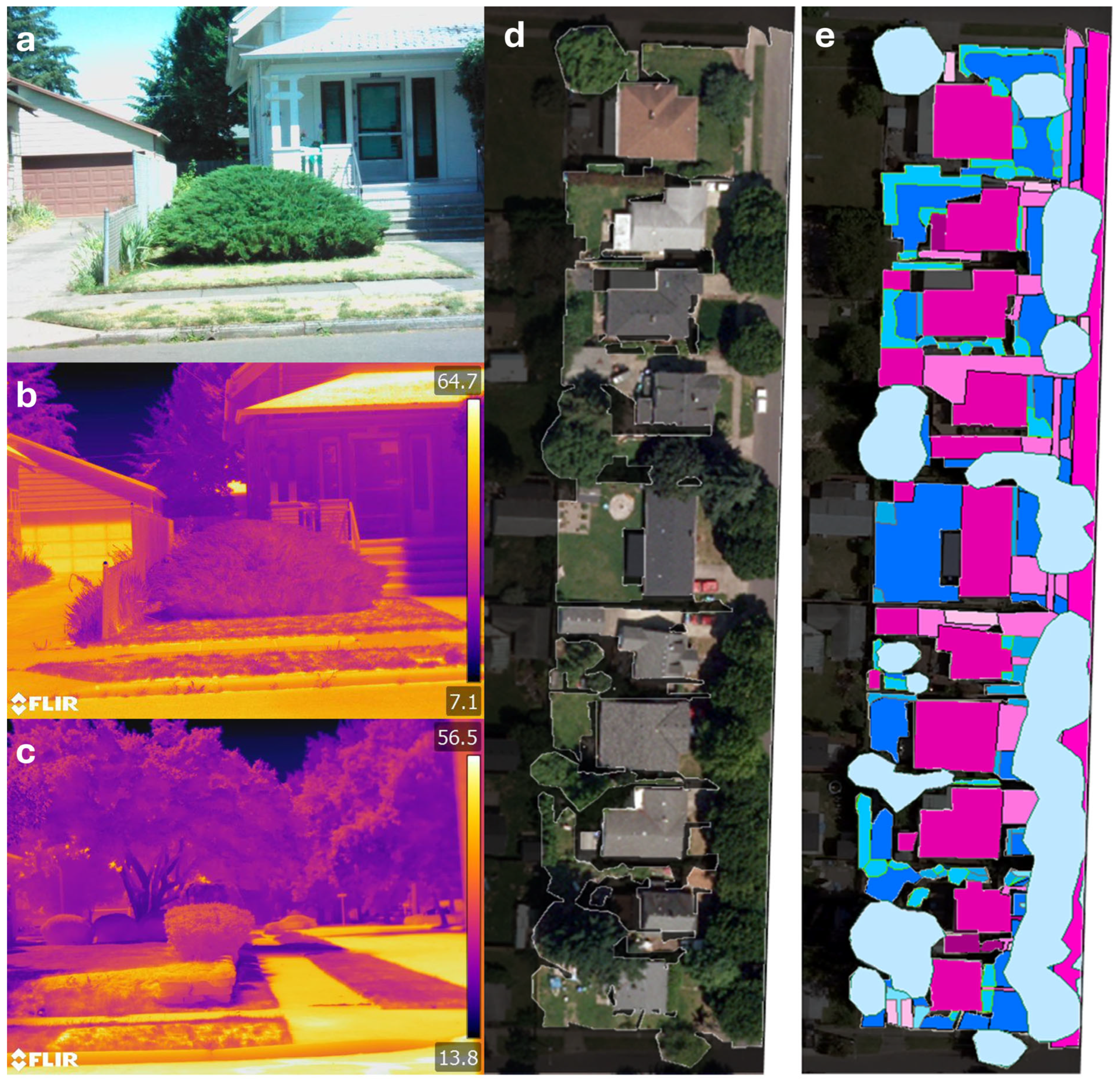
2.2. Thermography and Air Temperature Data Collection
2.3. Thermal Image Analysis
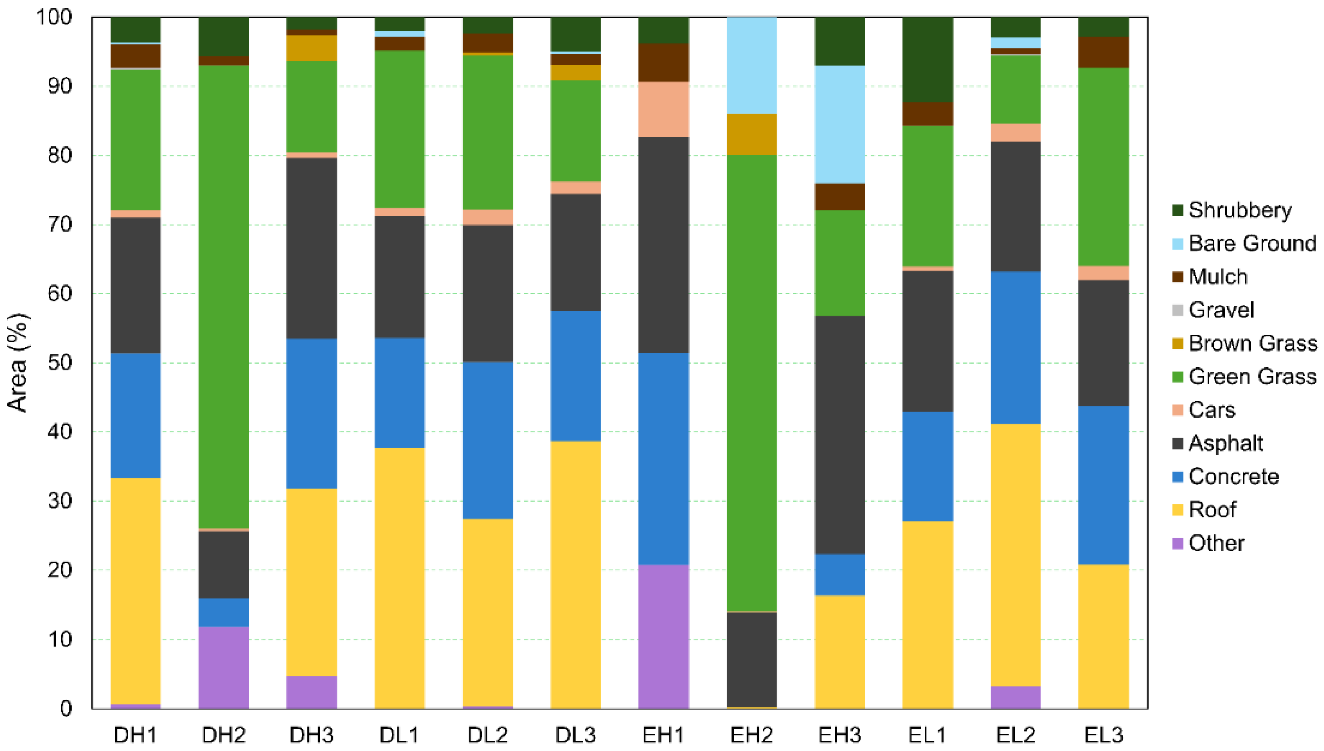
2.4. Surface Cover Mapping
2.5. Surface Cover Shade Apportioning and Average Streetscape Surface Temperatures
2.6. Statistical Hypothesis Testing and Temperature Modeling
3. Results
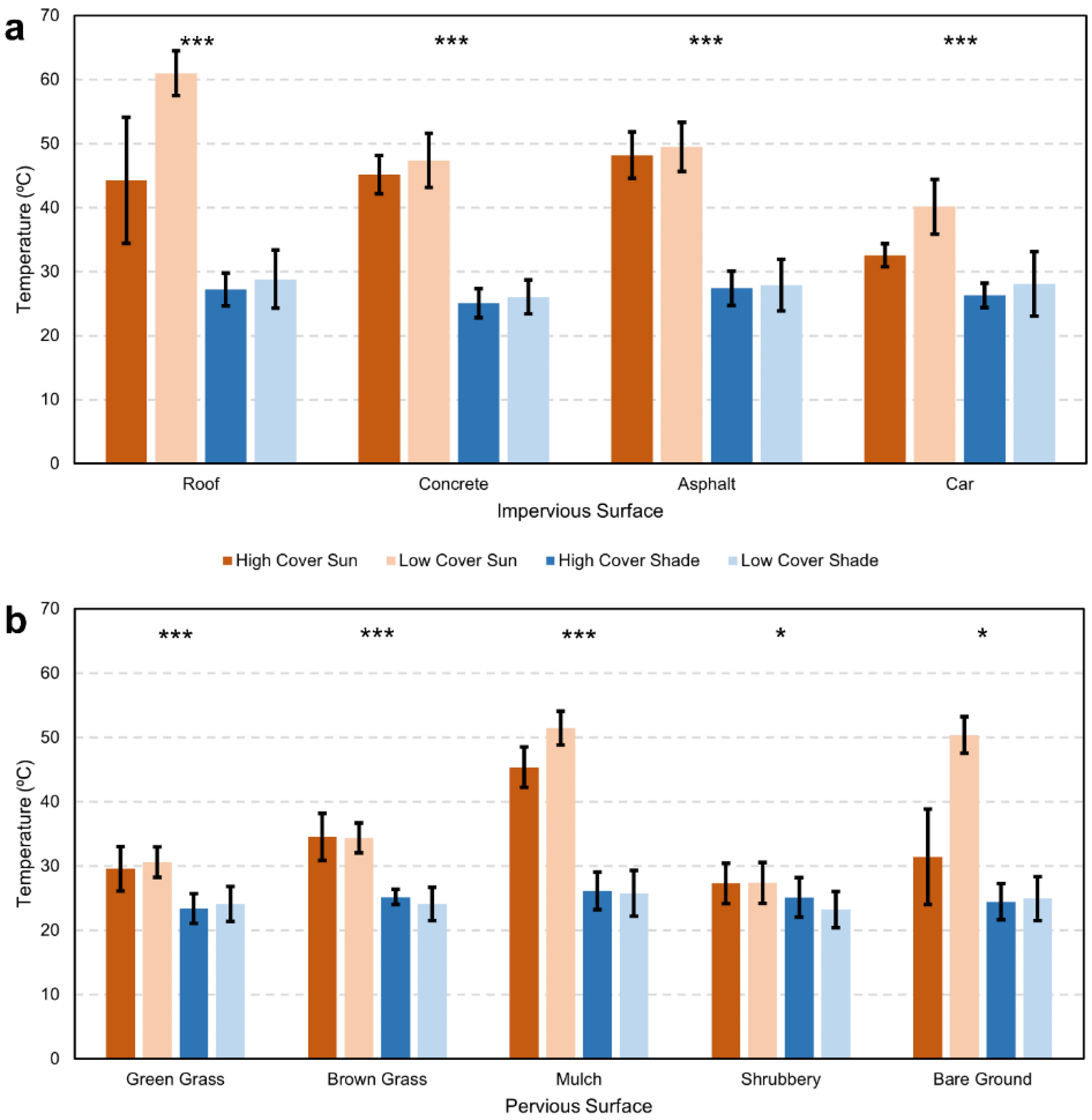
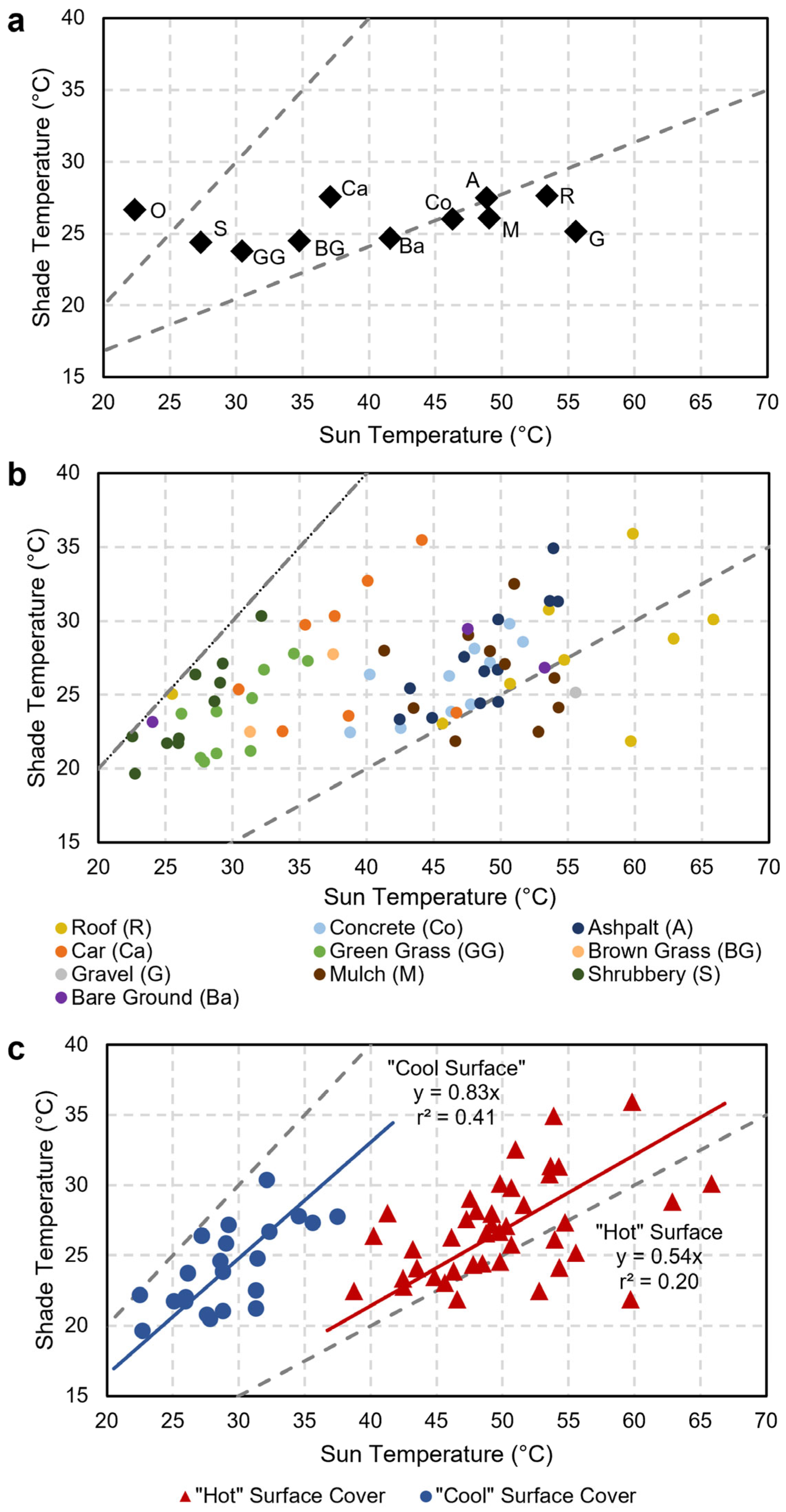
3.1. Surface Cover Types, Shading, and Temperature Variations
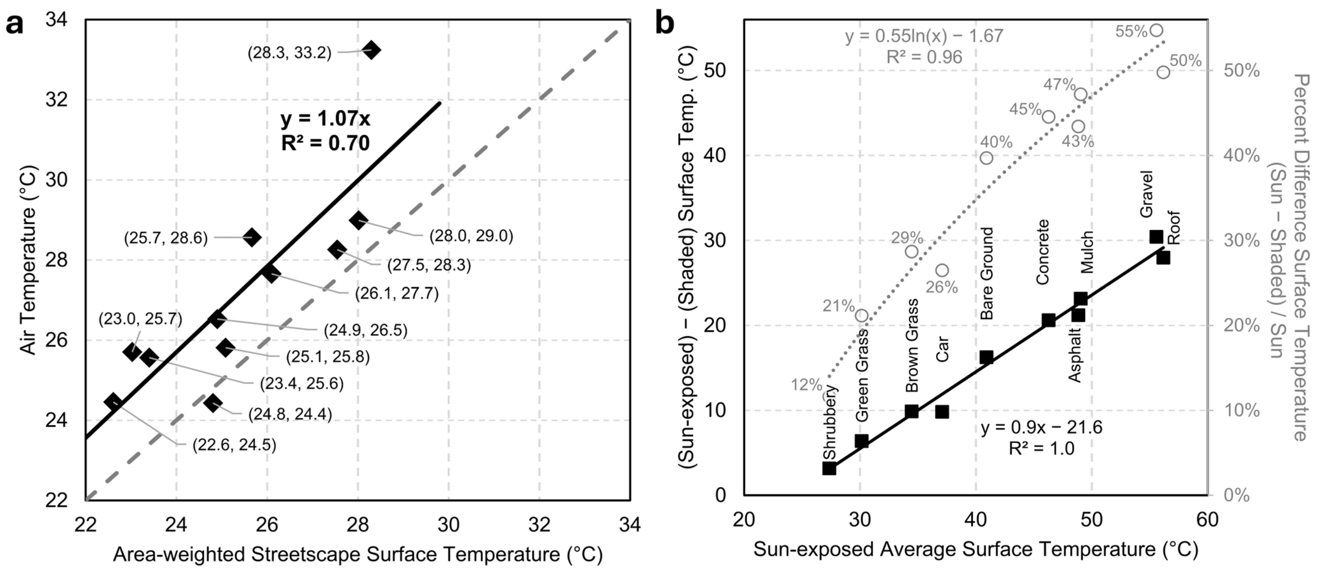
3.2. Surface-to-Air Temperature Relationships
4. Discussion
4.1. Interpretation and Application of Results
4.2. Implications for Mitigating Urban Heat by Plot-Scale Landscaping Choices
4.3. Implications for Predicting Urban Air Temperatures from Remote Sensing Data
5. Conclusions
Author Contributions
Funding
Data Availability Statement
Acknowledgments
Conflicts of Interest
References
- United Nations, Department of Economic and Social Affairs, & Population Division. World Urbanization Prospects: The 2018 Revision; United Nations: New York, NY, USA, 2018; Volume 12. [Google Scholar] [CrossRef]
- Mavrogianni, A.; Davies, M.; Batty, M.; Belcher, S.E.; Bohnenstengel, S.I.; Carruthers, D.; Chalabi, Z.; Croxford, B.; Demanuele, C.; Evans, S.; et al. The comfort, energy and health implications of London’s urban heat island. Build. Serv. Eng. Res. Technol. 2011, 32, 35–52. [Google Scholar] [CrossRef]
- Möhlenkamp, M.; Schmidt, M.; Wesseling, M.; Wick, A.; Gores, I.; Müller, D. Thermal comfort in environments with different vertical air temperature gradients. Indoor Air 2019, 29, 101–111. [Google Scholar] [CrossRef]
- Pantavou, K.; Theoharatos, G.; Mavrakis, A.; Santamouris, M. Evaluating thermal comfort conditions and health responses during an extremely hot summer in Athens. Build. Environ. 2011, 46, 339–344. [Google Scholar] [CrossRef]
- Watkins, R.; Palmer, J.; Kolokotroni, M. Increased temperature and intensification of the urban heat island: Implications for human comfort and urban design. Built Environ. 2007, 33, 85–96. [Google Scholar] [CrossRef]
- Wilby, R.L. A Review of Climate Change. Built Environ. 2006, 33, 31–45. [Google Scholar] [CrossRef]
- Arnfield, A.J. Two decades of urban climate research: A review of turbulence, exchanges of energy and water, and the urban heat island. Int. J. Clim. A J. R. Meteorol. Society 2003, 23, 1–26. [Google Scholar] [CrossRef]
- Voogt, J.A.; Oke, T.R. Thermal remote sensing of urban climates. Remote Sens. Environ. 2003, 86, 370–384. [Google Scholar] [CrossRef]
- Hou, P.; Chen, Y.; Qiao, W.; Cao, G.; Jiang, W.; Li, J. Near-surface air temperature retrieval from satellite images and influence by wetlands in urban region. Theor. Appl. Clim. 2013, 111, 109–118. [Google Scholar] [CrossRef]
- Mirzaei, P.A. Recent challenges in modeling of urban heat island. Sustain. Cities Soc. 2015, 19, 200–206. [Google Scholar] [CrossRef]
- Mirzaei, P.A.; Haghighat, F. Approaches to study urban heat island–abilities and limitations. Build. Environ. 2010, 45, 2192–2201. [Google Scholar] [CrossRef]
- Chatterjee, S.; Khan, A.; Dinda, A.; Mithun, S.; Khatun, R.; Akbari, H.; Kusaka, H.; Mitra, C.; Bhatti, S.S.; Van Doan, Q.; et al. Simulating micro-scale thermal interactions in different building environments for mitigating urban heat islands. Sci. Total Environ. 2019, 663, 610–631. [Google Scholar] [CrossRef] [PubMed]
- Bahi, H.; Mastouri, H.; Radoine, H. Review of methods for retrieving urban heat islands. Mater. Today Proc. 2020, 27, 3004–3009. [Google Scholar] [CrossRef]
- Chandrappa, A.K.; Biligiri, K.P. Development of Pavement-Surface Temperature Predictive Models: Parametric Approach. J. Mater. Civ. Eng. 2016, 28, 04015143. [Google Scholar] [CrossRef]
- McGregor, G.R.; Vanos, J.K. Heat: A primer for public health researchers. Public Health 2018, 161, 138–146. [Google Scholar] [CrossRef]
- Middel, A.; Selover, N.; Hagen, B.; Chhetri, N. Impact of shade on outdoor thermal comfort—A seasonal field study in Tempe, Arizona. Int. J. Biometeorol. 2016, 60, 1849–1861. [Google Scholar] [CrossRef]
- Akbari, H. Shade trees reduce building energy use and CO2 emissions from power plants. Environ. Pollut. 2002, 116 (Suppl. 1), S119–S126. [Google Scholar] [CrossRef]
- Wang, Z.H.; Zhao, X.; Yang, J.; Song, J. Cooling and energy saving potentials of shade trees and urban lawns in a desert city. Appl. Energy 2016, 161, 437–444. [Google Scholar] [CrossRef]
- Jung, S.; Yoon, S. Analysis of the Effects of Floor Area Ratio Change in Urban Street Canyons on Microclimate and Particulate Matter. Energies 2021, 14, 714. [Google Scholar] [CrossRef]
- Blount, K.; Wolfand, J.M.; Bell, C.D.; Ajami, N.K.; Hogue, T.S. Satellites to Sprinklers: Assessing the Role of Climate and Land Cover Change on Patterns of Urban Outdoor Water Use. Water Resour. Res. 2021, 57, e2020WR027587. [Google Scholar] [CrossRef]
- Gao, K.; Santamouris, M.; Feng, J. On the cooling potential of irrigation to mitigate urban heat island. Sci. Total Environ. 2020, 740, 139754. [Google Scholar] [CrossRef]
- Walsh, C.J.; Booth, D.B.; Burns, M.J.; Fletcher, T.D.; Hale, R.L.; Hoang, L.N.; Livingston, G.; Rippy, M.A.; Roy, A.H.; Scoggins, M.; et al. Principles for urban stormwater management to protect stream ecosystems. Freshw. Sci. 2016, 35, 398–411. [Google Scholar] [CrossRef]
- Berland, A.; Shiflett, S.A.; Shuster, W.D.; Garmestani, A.S.; Goddard, H.C.; Herrmann, D.L.; Hopton, M.E. The role of trees in urban stormwater management. Landsc. Urban Plan. 2017, 162, 167–177. [Google Scholar] [CrossRef] [PubMed]
- Panos, C.L.; Hogue, T.S.; Gilliom, R.L.; McCray, J.E. High-resolution Modeling of Infill Development Impact on Urban Stormwater Dynamics High-resolution Modeling of Infill Development Impact on Stormwater Dynamics in Denver, Colorado. J. Sustain. Water Built Environ. 2018, 4, 04018009. [Google Scholar] [CrossRef]
- Litvak, E.; Manago, K.F.; Hogue, T.S.; Pataki, D.E. Evapotranspiration of urban landscapes in Los Angeles, California at the municipal scale. J. Am. Water Resour. Assoc. 2017, 53, 4236–4252. [Google Scholar] [CrossRef]
- Zipper, S.C.; Schatz, J.; Kucharik, C.J.; Loheide, S.P. Urban heat island-induced increases in evapotranspirative demand. Geophys. Res. Lett. 2017, 44, 873–881. [Google Scholar] [CrossRef]
- Rao, P.K. Remote sensing of urban heat islands from an environmental satellite. Bull. Amer. Meteor. Soc. 1972, 53, 647–648. [Google Scholar]
- Matson, M.; Mcclain, E.P.; McGinnis, D.F.; Pritchard, J.A. Satellite Detection of Urban Heat Islands. Mon. Wea. Rev. 1978, 106, 1725–1734. [Google Scholar] [CrossRef]
- Price, J.C. Assessment of the Urban Heat Island Effect Through the Use of Satellite Data. Mon. Weather Rev. 1979, 107, 1554–1557. [Google Scholar] [CrossRef]
- Roth, M.; Oke, T.R.; Emery, W.J. Satellite-derived urban heat islands from three coastal cities and the utilization of such data in urban climatology. Int. J. Remote Sens. 1989, 10, 1699–1720. [Google Scholar] [CrossRef]
- Lambert-Habib, M.L.; Hidalgo, J.; Fedele, C.; Lemonsu, A.; Bernard, C. How is climatic adaptation taken into account by legal tools? Introduction of water and vegetation by French town planning documents. Urban Clim. 2013, 4, 16–34. [Google Scholar] [CrossRef]
- Lin, J.; Brown, R.D. Integrating Microclimate into Landscape Architecture for Outdoor Thermal Comfort: A Systematic Review. Land 2021, 10, 196. [Google Scholar] [CrossRef]
- Park, Y.; Guldmann, J.M.; Liu, D. Impacts of tree and building shades on the urban heat island: Combining remote sensing, 3D digital city and spatial regression approaches. Comput. Environ. Urban Syst. 2021, 88, 101655. [Google Scholar] [CrossRef]
- Li, X.; Li, W.; Middel, A.; Harlan, S.L.; Brazel, A.J.; Turner Ii, B.L. Remote sensing of the surface urban heat island and land architecture in Phoenix, Arizona: Combined effects of land composition and configuration and cadastral–demographic–economic factors. Remote Sens. Environ. 2016, 174, 233–243. [Google Scholar] [CrossRef]
- Osborne, P.E.; Alvares-Sanches, T. Quantifying how landscape composition and configuration affect urban land surface temperatures using machine learning and neutral landscapes. Comput. Environ. Urban Syst. 2019, 76, 80–90. [Google Scholar] [CrossRef]
- Parlow, E.; Vogt, R.; Feigenwinter, C. The urban heat island of Basel—Seen from different perspectives. DIE ERDE–J. Geogr. Soc. Berl. 2014, 145, 96–110. [Google Scholar] [CrossRef]
- Wu, H.; Li, Z.L. Scale issues in remote sensing: A review on analysis, processing and modeling. Sensors 2009, 9, 1768–1793. [Google Scholar] [CrossRef]
- Zhou, D.; Xiao, J.; Bonafoni, S.; Berger, C.; Deilami, K.; Zhou, Y.; Frolking, S.; Yao, R.; Qiao, Z.; Sobrino, J.A. Satellite remote sensing of surface urban heat islands: Progress, challenges, and perspectives. Remote Sens. 2018, 11, 48. [Google Scholar] [CrossRef]
- Du, M.; Li, N.; Hu, T.; Yang, Q.; Chakraborty, T.C.; Venter, Z.; Yao, R. Daytime cooling efficiencies of urban trees derived from land surface temperature are much higher than those for air temperature. Environ. Res. Lett. 2024, 19, 044037. [Google Scholar] [CrossRef]
- Zipper, S.C.; Schatz, J.; Singh, A.; Kucharik, C.J.; Townsend, P.A.; Loheide, S.P. Urban heat island impacts on plant phenology: Intra-urban variability and response to land cover. Environ. Res. Lett. 2016, 11, 054023. [Google Scholar] [CrossRef]
- Nichol, J.E.; Fung, W.Y.; Lam, K.; Wong, M.S. Urban heat island diagnosis using ASTER satellite images and ‘in situ’ air temperature. Atmos. Res. 2009, 94, 276–284. [Google Scholar] [CrossRef]
- Hart, M.A.; Sailor, D.J. Quantifying the influence of land-use and surface characteristics on spatial variability in the urban heat island. Theor. Appl. Climatol. 2009, 95, 397–406. [Google Scholar] [CrossRef]
- Tsin, P.K.; Knudby, A.; Krayenhoff, E.S.; Ho, H.C.; Brauer, M.; Henderson, S.B. Microscale mobile monitoring of urban air temperature. Urban Clim. 2016, 18, 58–72. [Google Scholar] [CrossRef]
- Makido, Y.; Shandas, V.; Ferwati, S.; Sailor, D. Daytime Variation of Urban Heat Islands: The Case Study of Doha, Qatar. Climate 2016, 4, 32. [Google Scholar] [CrossRef]
- Shandas, V.; Voelkel, J.; Rao, M.; George, L. Integrating High-Resolution Datasets to Target Mitigation Efforts for Improving Air Quality and Public Health in Urban Neighborhoods. Int. J. Environ. Res. Public Health 2016, 13, 790. [Google Scholar] [CrossRef]
- Voelkel, J.; Shandas, V. Towards Systematic Prediction of Urban Heat Islands: Grounding Measurements, Assessing Modeling Techniques. Climate 2017, 5, 41. [Google Scholar] [CrossRef]
- Ziter, C.D.; Pedersen, E.J.; Kucharik, C.J.; Turner, M.G. Scale-dependent interactions between tree canopy cover and impervious surfaces reduce daytime urban heat during summer. Proc. Natl. Acad. Sci. USA 2019, 116, 7575–7580. [Google Scholar] [CrossRef]
- Yan, C.; Guo, Q.; Li, H.; Li, L.; Qiu, G.Y. Quantifying the cooling effect of urban vegetation by mobile traverse method: A local-scale urban heat island study in a subtropical megacity. Build. Environ. 2020, 169, 106541. [Google Scholar] [CrossRef]
- Rodríguez, L.R.; Ramos, J.S.; Félix, J.L.M.; Domínguez, S.Á. Urban-scale air temperature estimation: Development of an empirical model based on mobile transects. Sustain. Cities Soc. 2020, 63, 102471. [Google Scholar] [CrossRef]
- Kousis, I.; Manni, M.; Pisello, A.L. Environmental mobile monitoring of urban microclimates: A review. Renew. Sustain. Energy Rev. 2022, 169, 112847. [Google Scholar] [CrossRef]
- Kaplan, S.; Peeters, A.; Erell, E. Predicting air temperature simultaneously for multiple locations in an urban environment: A bottom up approach. Appl. Geogr. 2016, 76, 62–74. [Google Scholar] [CrossRef]
- Moffett, K.B.; Makido, Y.; Shandas, V. Urban-Rural Surface Temperature Deviation and Intra-Urban Variations Contained by an Urban Growth Boundary. Remote Sens. 2019, 11, 2683. [Google Scholar] [CrossRef]
- Kottmeier, C.; Biegert, C.; Corsmeier, U. Effects of Urban Land Use on Surface Temperature in Berlin: Case Study. J. Urban Plan. Dev. 2007, 133, 128–137. [Google Scholar] [CrossRef]
- Dugord, P.A.; Lauf, S.; Schuster, C.; Kleinschmit, B. Land use patterns, temperature distribution, and potential heat stress risk—The case study Berlin, Germany. Comput. Environ. Urban Syst. 2014, 48, 86–98. [Google Scholar] [CrossRef]
- Kumar, D.; Shekhar, S. Statistical analysis of land surface temperature-vegetation indexes relationship through thermal remote sensing. Ecotoxicol. Environ. Saf. 2015, 121, 39–44. [Google Scholar] [CrossRef]
- Wang, K.; Jiang, S.; Wang, J.; Zhou, C.; Wang, X.; Lee, X. Comparing the diurnal and seasonal variabilities of atmospheric and surface urban heat islands based on the Beijing urban meteorological network. J. Geophys. Res. Atmos. 2017, 122, 2131–2154. [Google Scholar] [CrossRef]
- Chen, Y.; Yu, S. Impacts of urban landscape patterns on urban thermal variations in Guangzhou, China. Int. J. Appl. Earth Obs. Geoinf. 2017, 54, 65–71. [Google Scholar] [CrossRef]
- Sun, Y.; Gao, C.; Li, J.; Li, W.; Ma, R. Examining urban thermal environment dynamics and relations to biophysical composition and configuration and socio-economic factors: A case study of the Shanghai metropolitan region. Sustain. Cities Soc. 2018, 40, 284–295. [Google Scholar] [CrossRef]
- Sanusi, R.; Johnstone, D.; May, P.; Livesley, S.J. Street Orientation and Side of the Street Greatly Influence the Microclimatic Benefits Street Trees Can Provide in Summer. J. Environ. Qual. 2016, 45, 167. [Google Scholar] [CrossRef]
- Menne, M.J.; Durre, I.; Korzeniewski, B.; McNeal, S.; Thomas, K.; Yin, X.; Anthony, S.; Ray, R.; Vose, R.S.; Gleason, B.E.; et al. Global Historical Climatology Network—Daily (GHCN-Daily), Version 3. J. Atmos. Oceanic Technol. 2012, 29, 897–910. [Google Scholar] [CrossRef]
- Kottek, M.; Grieser, J.; Beck, C.; Rudolf, B.; Rubel, F. World map of the Köppen-Geiger climate classification updated. Meteorol. Z. 2006, 15, 259–263. [Google Scholar] [CrossRef]
- NCDC. 1991–2020 Monthly Climate Normals, PORTLAND INTL APT: Portland Weather Forecast Office, OR US. 2020. Available online: https://www.ncei.noaa.gov/access/us-climate-normals/#dataset=normals-monthly&timeframe=30&location=OR&station=USW00024229 (accessed on 15 April 2025).
- NCDC. 1991–2020 Hourly Climate Normals, June 28, PORTLAND INTL APT: Portland Weather Forecast Office, OR US. 2020. Available online: https://www.ncei.noaa.gov/access/us-climate-normals/#dataset=normals-hourly&timeframe=30&station=USW00024229&month=5&day=27 (accessed on 15 April 2025).
- Google. Portland, Oregon. 2016. Available online: https://earth.google.com (accessed on 12 July 2016).
- Brandani, G.; Napoli, M.; Massetti, L.; Petralli, M.; Orlandini, S. Urban Soil: Assessing Ground Cover Impact on Surface Temperature and Thermal Comfort. J. Environ. Qual. 2016, 45, 90–97. [Google Scholar] [CrossRef] [PubMed]
- Napoli, M.; Massetti, L.; Brandani, G.; Petralli, M.; Orlandini, S. Modeling Tree Shade Effect on Urban Ground Surface Temperature. J. Environ. Qual. 2016, 45, 146. [Google Scholar] [CrossRef] [PubMed]
- Pattnaik, N.; Honold, M.; Franceschi, E.; Moser-Reischl, A.; Rötzer, T.; Pretzsch, H.; Pauleit, S.; Rahman, M.A. Growth and cooling potential of urban trees across different levels of imperviousness. J. Environ. Manag. 2024, 361, 121242. [Google Scholar] [CrossRef]
- Chen, Y.; Wu, J.; Yu, K.; Wang, D. Evaluating the impact of the building density and height on the block surface temperature. Build. Environ. 2020, 168, 106493. [Google Scholar] [CrossRef]
- Li, Q.; Wang, Z.-H. Large-eddy simulation of the impact of urban trees on momentum and heat fluxes. Agric. For. Meteorol. 2018, 255, 44–56. [Google Scholar] [CrossRef]
- Azevedo, J.A.; Chapman, L.; Muller, C.L. Quantifying the daytime and night-time urban heat Island in Birmingham, UK: A comparison of satellite derived land surface temperature and high resolution air temperature observations. Remote Sens. 2016, 8, 153. [Google Scholar] [CrossRef]
- Cao, J.; Zhou, W.; Zheng, Z.; Ren, T.; Wang, W. Within-city spatial and temporal heterogeneity of air temperature and its relationship with land surface temperature. Landsc. Urban Plan. 2021, 206, 103979. [Google Scholar] [CrossRef]
- Widyasamratri, H.; Souma, K.; Suetsugi, T.; Ishidaira, H.; Ichikawa, Y.; Kobayashi, H.; Inagaki, I. A Comparison Air Temperature and Land Surface Temperature to Detect an Urbanization Effect in Jakarta, Indonesia. In Proceedings of the 34th Asian Conference on Remote Sensing, Bali, Indoneisa, 20–24 October 2013. [Google Scholar]
- Nichol, J.E.; To, P.H. Temporal characteristics of thermal satellite images for urban heat stress and heat island mapping. ISPRS J. Photogramm. Remote Sens. 2012, 74, 153–162. [Google Scholar] [CrossRef]
- Rahman, M.A.; Dervishi, V.; Moser-Reischl, A.; Ludwig, F.; Pretzsch, H.; Rötzer, T.; Pauleit, S. Comparative analysis of shade and underlying surfaces on cooling effect. Urban For. Urban Green. 2021, 63, 127223. [Google Scholar] [CrossRef]
- Imhoff, M.L.; Zhang, P.; Wolfe, R.E.; Bounoua, L. Remote sensing of the urban heat island effect across biomes in the continental USA. Remote Sens. Environ. 2010, 114, 504–513. [Google Scholar] [CrossRef]
- Yuan, F.; Bauer, M.E. Comparison of impervious surface area and normalized difference vegetation index as indicators of surface urban heat island effects in Landsat imagery. Remote Sens. Environ. 2007, 106, 375–386. [Google Scholar] [CrossRef]
- Zhang, Z.; Ji, M.; Shu, J.; Deng, Z.; Wu, Y. Surface urban heat island in Shanghai, China: Examining the relationship between land surface temperature and impervious surface fractions derived from Landsat ETM+ imagery. Int. Arch. Photogramm. Remote Sens. Spat. Inf. Sci. 2008, 37, 601–606. [Google Scholar]
- Shiflett, S.A.; Liang, L.L.; Crum, S.M.; Feyisa, G.L.; Wang, J.; Jenerette, G.D. Variation in the urban vegetation, surface temperature, air temperature nexus. Sci. Total Environ. 2017, 579, 495–505. [Google Scholar] [CrossRef] [PubMed]
- Melaas, E.K.; Wang, J.A.; Miller, D.L.; Friedl, M.A. Interactions between urban vegetation and surface urban heat islands: A case study in the Boston metropolitan region. Environ. Res. Lett. 2016, 11, 054020. [Google Scholar] [CrossRef]
- Buyantuyev, A.; Wu, J. Urban heat islands and landscape heterogeneity: Linking spatiotemporal variations in surface temperatures to land-cover and socioeconomic patterns. Landsc. Ecol. 2010, 25, 17–33. [Google Scholar] [CrossRef]
- Estoque, R.C.; Murayama, Y.; Myint, S.W. Effects of landscape composition and pattern on land surface temperature: An urban heat island study in the megacities of Southeast Asia. Sci. Total Environ. 2017, 577, 349–359. [Google Scholar] [CrossRef]
- Guhathakurta, S.; Gober, P. Residential land use, the Urban heat island, and water use in phoenix: A path analysis. J. Plan. Educ. Res. 2010, 30, 40–51. [Google Scholar] [CrossRef]
- Shashua-Bar, L.; Pearlmutter, D.; Erell, E. The cooling efficiency of urban landscape strategies in a hot dry climate. Landsc. Urban Plan. 2009, 92, 179–186. [Google Scholar] [CrossRef]
- Konarska, J.; Uddling, J.; Holmer, B.; Lutz, M.; Lindberg, F.; Pleijel, H.; Thorsson, S. Transpiration of urban trees and its cooling effect in a high latitude city. Int. J. Biometeorol. 2016, 60, 159–172. [Google Scholar] [CrossRef]
- Oliveira, S.; Andrade, H.; Vaz, T. The cooling effect of green spaces as a contribution to the mitigation of urban heat: A case study in Lisbon. Build. Environ. 2011, 46, 2186–2194. [Google Scholar] [CrossRef]
- Huttner, S.; Bruse, M.; Dostal, P. Using ENVI-met to simulate the impact of global warming on the mi- croclimate in central European cities. In Proceedings of the 5th Japanese-German Meeting on Urban Climatology, Freiburg, Germany, 6–11 October 2008; Volume 18, pp. 307–312. [Google Scholar]
- Yan, H.; Dong, L. The impacts of land cover types on urban outdoor thermal environment: The case of Beijing, China. J. Environ. Health Sci. Eng. 2015, 13, 43. [Google Scholar] [CrossRef] [PubMed]
- Alonzo, M.; Baker, M.E.; Gao, Y.; Shandas, V. Spatial configuration and time of day impact the magnitude of urban tree canopy cooling. Environ. Res. Lett. 2021, 16, 084028. [Google Scholar] [CrossRef]
- Connors, J.P.; Galletti, C.S.; Chow, W.T.L. Landscape configuration and urban heat island effects: Assessing the relationship between landscape characteristics and land surface temperature in Phoenix, Arizona. Landsc. Ecol. 2013, 28, 271–283. [Google Scholar] [CrossRef]
- Keith, L.; Meerow, S.; Wagner, T. Planning for Extreme Heat: A Review. J. Extrem. Events 2019, 6, 2050003. [Google Scholar] [CrossRef]


| ID | Street Tree Type | Canopy Density | Location | Date Imaged | Times Imaged | Site Area (m2) |
|---|---|---|---|---|---|---|
| DL1 | Deciduous | Low | East of N Exeter Ave between N Newark St and N Hudson St | 27 June | 3:46–3:55 p.m. | 4316 |
| DL2 | Deciduous | Low | East of N Chautauqua Blvd between N Winchell St and N Baldwin St | 28 June | 2:16–2:28 p.m. | 14,645 |
| DL3 | Deciduous | Low | East of SE 73rd Ave between SE Raymond St and SE Schiller St | 29 June | 2:23–2:32 p.m. | 4348 |
| DH1 | Deciduous | High | West of N Exeter Ave between N Newark St and N Hudson St | 27 June | 3:29–3:45 p.m. | 4484 |
| DH2 | Deciduous | High | West of N Chautauqua Blvd between N Winchell St and N Baldwin St | 28 June | 2:00–2:14 p.m. | 5689 |
| DH3 | Deciduous | High | Both sides of SE 72nd Ave between SE Schiller St and SE Foster Rd | 29 June | 2:44–2:56 p.m. | 4573 |
| EL1 | Evergreen | Low | East of 135th Ave between SE Yamhill St and SE Salmon St | 28 June | 4:35–4:39 p.m. | 2301 |
| EL2 | Evergreen | Low | West of N Exeter Ave between N Fessenden St and N Cecelia St | 28 June | 3:56–4:04 p.m. | 6635 |
| EL3 | Evergreen | Low | East of N Exeter Ave between N Fessenden St and N Cecelia St | 28 June | 3:13–3:19 p.m. | 904 |
| EH1 | Evergreen | High | West of NE 22nd Ave between NE Irving St and NE Hoyt St | 29 June | 1:39–2:20 p.m. | 3198 |
| EH2 | Evergreen | High | West of SE 50th Ave between SE Steele St and SE Insley St | 27 June | 1:08–2:49 p.m. | 3522 |
| EH3 | Evergreen | High | East of SW 45th Ave between SW Vesta Dr and SW Vacuna St | 27 June | 1:52–2:21 p.m. | 4065 |
| Sun-Exposed Urban Surface Cover Type | ||||||||||
|---|---|---|---|---|---|---|---|---|---|---|
| Site | Roof | Concrete | Asphalt | Car | Green Grass | Brown Grass | Mulch | Shrubs | Bare Ground | Gravel |
| DH1 | 53.6 | 48.0 | 54.3 | 35.4 | 35.6 | 39.7 | 47.6 | 32.1 | ||
| DH2 | 45.6 | 40.2 | 49.8 | 32.0 | 27.6 | 26.0 | ||||
| DH3 | 50.7 | 42.5 | 44.8 | 30.4 | 31.3 | 31.3 | 43.5 | 22.5 | 24.0 | |
| EH1 | 46.1 | 43.2 | 32.3 | 49.2 | 27.2 | |||||
| EH2 | 46.0 | 45.4 | 47.3 | 27.3 | 32.6 | 38.9 | ||||
| EH3 | 48.8 | 49.8 | 26.2 | 41.3 | 28.6 | |||||
| DL1 | 65.8 | 51.6 | 53.9 | 44.1 | 34.5 | 37.5 | 51.0 | 32.4 | 47.5 | |
| DL2 | 59.7 | 47.8 | 48.8 | 38.6 | 28.8 | 31.1 | 52.8 | 25.9 | ||
| DL3 | 62.9 | 46.3 | 48.5 | 46.7 | 28.8 | 33.8 | 54.3 | 25.1 | ||
| EL1 | 54.7 | 38.7 | 42.4 | 33.7 | 27.8 | 46.6 | 22.7 | |||
| EL2 | 62.9 | 49.2 | 49.8 | 40.1 | 32.3 | 35.2 | 50.3 | 29.2 | 53.3 | |
| EL3 | 59.8 | 50.7 | 53.7 | 37.6 | 31.4 | 54.0 | 29.0 | 55.6 | ||
| D avg. | 56.4 | 46.1 | 50.0 | 37.9 | 31.1 | 34.7 | 49.8 | 27.3 | 35.8 | |
| E avg. | 55.9 | 46.5 | 47.7 | 35.9 | 29.0 | 33.9 | 48.3 | 27.4 | 46.1 | 55.6 |
| H avg. | 49.0 | 45.2 | 48.2 | 32.5 | 29.6 | 34.5 | 45.4 | 27.3 | 31.4 | |
| L avg. | 61.0 | 47.4 | 49.5 | 40.1 | 30.6 | 34.4 | 51.5 | 27.4 | 50.4 | 55.6 |
| all avg. | 56.2 | 46.3 | 48.8 | 37.1 | 29.9 | 34.5 | 48.7 | 27.3 | 39.2 | 55.6 |
| Shaded Urban Surface Cover Type | ||||||||||
| Site | Roof | Concrete | Asphalt | Car | Green Grass | Brown Grass | Mulch | Shrubs | Bare Ground | Gravel |
| DH1 | 30.8 | 28.1 | 31.3 | 29.8 | 27.3 | 29.1 | 30.4 | 29.1 | ||
| DH2 | 23.1 | 26.4 | 24.5 | 20.8 | 21.4 | 22.1 | 20.4 | |||
| DH3 | 25.8 | 22.8 | 23.5 | 25.4 | 21.2 | 22.5 | 24.1 | 22.2 | 23.2 | |
| EH1 | 26.3 | 25.4 | 23.8 | 28.0 | 26.4 | 24.8 | ||||
| EH2 | 26.3 | 27.6 | 26.8 | 23.8 | 24.8 | 24.8 | ||||
| EH3 | 25.1 | 26.3 | 30.1 | 24.9 | 23.7 | 28.0 | 24.6 | |||
| DL1 | 30.1 | 28.6 | 34.9 | 35.5 | 27.8 | 27.8 | 32.5 | 29.5 | ||
| DL2 | 21.9 | 24.4 | 26.6 | 23.6 | 21.1 | 22.5 | 21.7 | 22.3 | ||
| DL3 | 23.9 | 24.4 | 23.8 | 23.9 | 24.2 | 21.7 | ||||
| EL1 | 27.4 | 22.5 | 23.4 | 22.5 | 20.5 | 21.7 | 21.9 | 19.7 | 21.1 | |
| EL2 | 28.8 | 27.2 | 26.7 | 32.7 | 26.7 | 27.1 | 27.1 | 26.9 | ||
| EL3 | 35.9 | 29.8 | 31.4 | 30.4 | 24.8 | 26.1 | 26.1 | 25.8 | 25.2 | |
| D avg. | 27.1 | 25.1 | 27.9 | 27.1 | 23.7 | 25.1 | 25.6 | 23.6 | 24.9 | |
| E avg. | 29.3 | 26.5 | 27.4 | 27.5 | 23.9 | 24.2 | 26.2 | 24.7 | 24.4 | 25.2 |
| H avg. | 27.2 | 25.1 | 27.4 | 26.3 | 23.4 | 23.7 | 26.1 | 25.1 | 24.5 | |
| L avg. | 28.8 | 26.1 | 27.9 | 28.1 | 24.1 | 25.2 | 25.7 | 23.2 | 24.9 | 25.2 |
| all avg. | 28.2 | 25.8 | 27.6 | 27.3 | 23.8 | 24.6 | 25.9 | 24.2 | 24.7 | 25.2 |
Disclaimer/Publisher’s Note: The statements, opinions and data contained in all publications are solely those of the individual author(s) and contributor(s) and not of MDPI and/or the editor(s). MDPI and/or the editor(s) disclaim responsibility for any injury to people or property resulting from any ideas, methods, instructions or products referred to in the content. |
© 2025 by the authors. Licensee MDPI, Basel, Switzerland. This article is an open access article distributed under the terms and conditions of the Creative Commons Attribution (CC BY) license (https://creativecommons.org/licenses/by/4.0/).
Share and Cite
Kubiniec, K.; Moffett, K.B.; Blount, K. Street-Scale Urban Air Temperatures Predicted by Simple High-Resolution Cover- and Shade-Weighted Surface Temperature Mosaics in a Variety of Residential Neighborhoods. Remote Sens. 2025, 17, 1932. https://doi.org/10.3390/rs17111932
Kubiniec K, Moffett KB, Blount K. Street-Scale Urban Air Temperatures Predicted by Simple High-Resolution Cover- and Shade-Weighted Surface Temperature Mosaics in a Variety of Residential Neighborhoods. Remote Sensing. 2025; 17(11):1932. https://doi.org/10.3390/rs17111932
Chicago/Turabian StyleKubiniec, Katarina, Kevan B. Moffett, and Kyle Blount. 2025. "Street-Scale Urban Air Temperatures Predicted by Simple High-Resolution Cover- and Shade-Weighted Surface Temperature Mosaics in a Variety of Residential Neighborhoods" Remote Sensing 17, no. 11: 1932. https://doi.org/10.3390/rs17111932
APA StyleKubiniec, K., Moffett, K. B., & Blount, K. (2025). Street-Scale Urban Air Temperatures Predicted by Simple High-Resolution Cover- and Shade-Weighted Surface Temperature Mosaics in a Variety of Residential Neighborhoods. Remote Sensing, 17(11), 1932. https://doi.org/10.3390/rs17111932