Estimation of Atmospheric Boundary Layer Turbulence Parameters over the South China Sea Based on Multi-Source Data

Abstract

Understanding optical turbulence within the atmospheric boundary layer (ABL) is essential for refining atmospheric motion analyses, enhancing numerical weather prediction models, and improving light propagation assessments. This study develops an optical turbulence model for the boundary layer over the South China Sea (SCS) by integrating multiple observational and reanalysis datasets, including ERA5 data from the European Center for Medium-Range Weather Forecasts (ECMWF), radiosonde observations, coherent Doppler wind lidar (CDWL), and ultrasonic anemometer (CSAT3) measurements. Utilizing Monin–Obukhov Similarity Theory (MOST) as the theoretical foundation, the model’s performance is evaluated by comparing its outputs with the observed diurnal cycle of near-surface optical turbulence. Error analysis indicates a root mean square error (RMSE) of less than 1 and a correlation coefficient exceeding 0.6, validating the model’s predictive capability. Moreover, this study demonstrates the feasibility of employing ERA5-derived temperature and pressure profiles as alternative inputs for optical turbulence modeling while leveraging CDWL’s high-resolution observational capacity for all-weather turbulence characterization. A comprehensive statistical analysis of the atmospheric refractive index structure constant ($C_n^2$) from November 2019 to September 2020 highlights its critical implications for optoelectronic system optimization and astronomical observatory site selection in the SCS region.

1. Introduction

The propagation of a light beam through the atmosphere is influenced by various turbulence-induced distortions, such as beam drift and intensity scintillation, which result from the dynamic and stochastic nature of atmospheric turbulence. Given that turbulence is an intrinsic property of atmospheric flow, a thorough understanding of its governing mechanisms and evolutionary patterns is essential for advancing research on atmospheric dynamics, refining numerical weather prediction models, and improving the accuracy of light propagation analyses [1,2,3,4].

Positioned between the surface and the free atmosphere, the atmospheric boundary layer (ABL) is the most dynamically active atmospheric region, characterized by strong surface interactions and pronounced sensitivity to diurnal weather variations. Accurate estimation of turbulence parameter variations within the ABL is, therefore, critical for understanding atmospheric processes, improving numerical weather prediction, and advancing environmental and engineering applications [5,6,7].

Numerous techniques and instruments have been developed to detect atmospheric optical turbulence, each with distinct advantages and limitations. The radiosonde is a relatively common method that can obtain some conventional meteorological parameters, yet it is hindered by a low temporal resolution and infrequent sampling [8]. Acoustic radar, when properly calibrated, can derive $C_n^2$ profiles; however, its applicability is restricted by significant acoustic signal attenuation and susceptibility to environmental noise contamination [9]. Unmanned aerial vehicles (UAVs) equipped with advanced sensor payloads enable high-precision turbulence measurements, facilitating the capture of micro-scale turbulence characteristics with superior detail. Nonetheless, real-time data acquisition remains challenging due to flight duration constraints and operational restrictions [10]. Additionally, the interpretation of turbulent statistics from ultrasonic anemometers can be hindered by the fetch conditions, and ultrasonic anemometers should be installed in open areas whenever possible [11].

By fitting extensive measured data, scientists have developed empirical models. However, the inherent complexity of meteorological parameters and locations has led to the development of various models to address these challenges, including the Hufnagel model [12], the Tatarski model [1,8], and the NOAA model [13]. The Tatarski model is widely used; nonetheless, discrepancies occur in estimating $C_n^2$ profiles when different outer scale models ($L_0$) are employed.

Coherent Doppler wind lidar (CDWL) is primarily employed to detect three-dimensional atmospheric wind patterns in urban boundary layers and low-altitude tropospheres with precision. Its applications encompass measuring vertical wind profiles, horizontal wind fields in complex terrains, land/sea fan power curve assessments, aircraft wake vortex monitoring and early warning, and atmospheric turbulence parameter inversion, among others. The reliability of CDWL has been validated in various fields [14,15,16,17]; however, it cannot acquire real-time temperature profiles. To mitigate this limitation, Zhang and Zhu et al. utilized the American 1976 standard atmospheric model as a substitute for measured temperature profiles to estimate atmospheric turbulence profiles [18,19]. Jiang et al. employed a microwave radiometer to measure temperature, subsequently estimating atmospheric turbulence profiles [20]. Qing et al. conducted vertical wind speed spectrum analysis using MST radar, calculated the Brunt–Väisälä frequency, and established a temperature inversion model based on its relationship with temperature, thereby deriving temperature profiles [21]. Therefore, utilizing ERA5 data such as temperature and pressure in conjunction with empirical models offers a straightforward and relatively cost-effective approach to calculating atmospheric turbulence parameters [22].

This study introduces a novel outer scale model tailored for the atmospheric boundary layer over oceanic regions. The model is developed by integrating measured radiosonde data with temperature and pressure information from ERA5 and is benchmarked against the HMNSP99 outer scale model. To validate its reliability, the model’s calculated results are compared with data obtained from ultrasonic anemometers. Additionally, the model is applied to Doppler lidar to analyze turbulence parameter variations in the South China Sea (SCS). The structure of this paper is as follows: Section 2 provides an overview of the experimental location, instrumentation, and data sources. Section 3 outlines the principles and methodologies employed in the experimental analysis. Section 4 presents the experimental findings and their implications. Finally, Section 5 offers a summary of the research outcomes and discusses potential future work.

2. Instrumentation and Data

2.1. Site Description

As depicted in Figure 1, the test site is located in the SCS region. The area highlighted in red indicates the designated release zone for the meteorosonde. This region experiences a climate characterized by high temperatures, with average sea surface temperatures ranging from 25 °C to 28 °C.

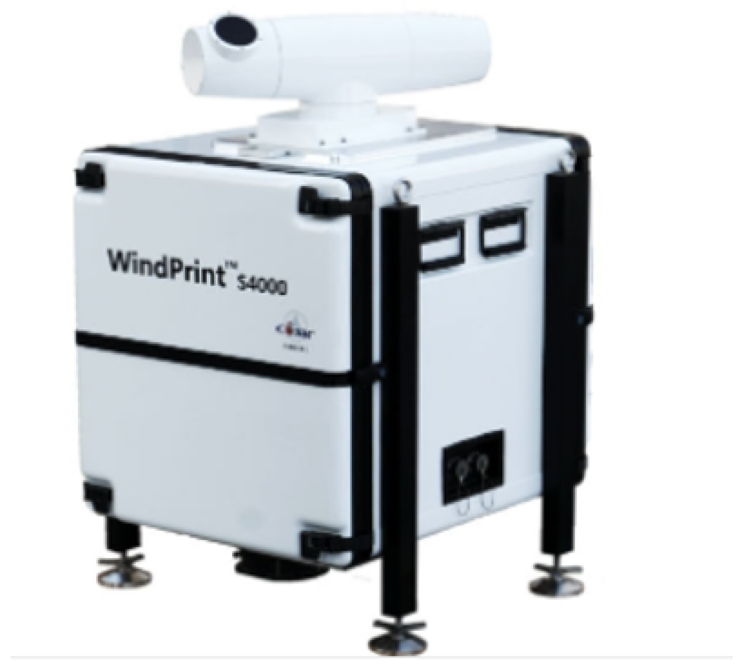
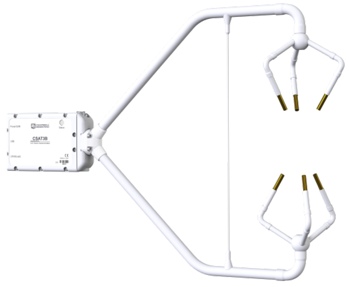
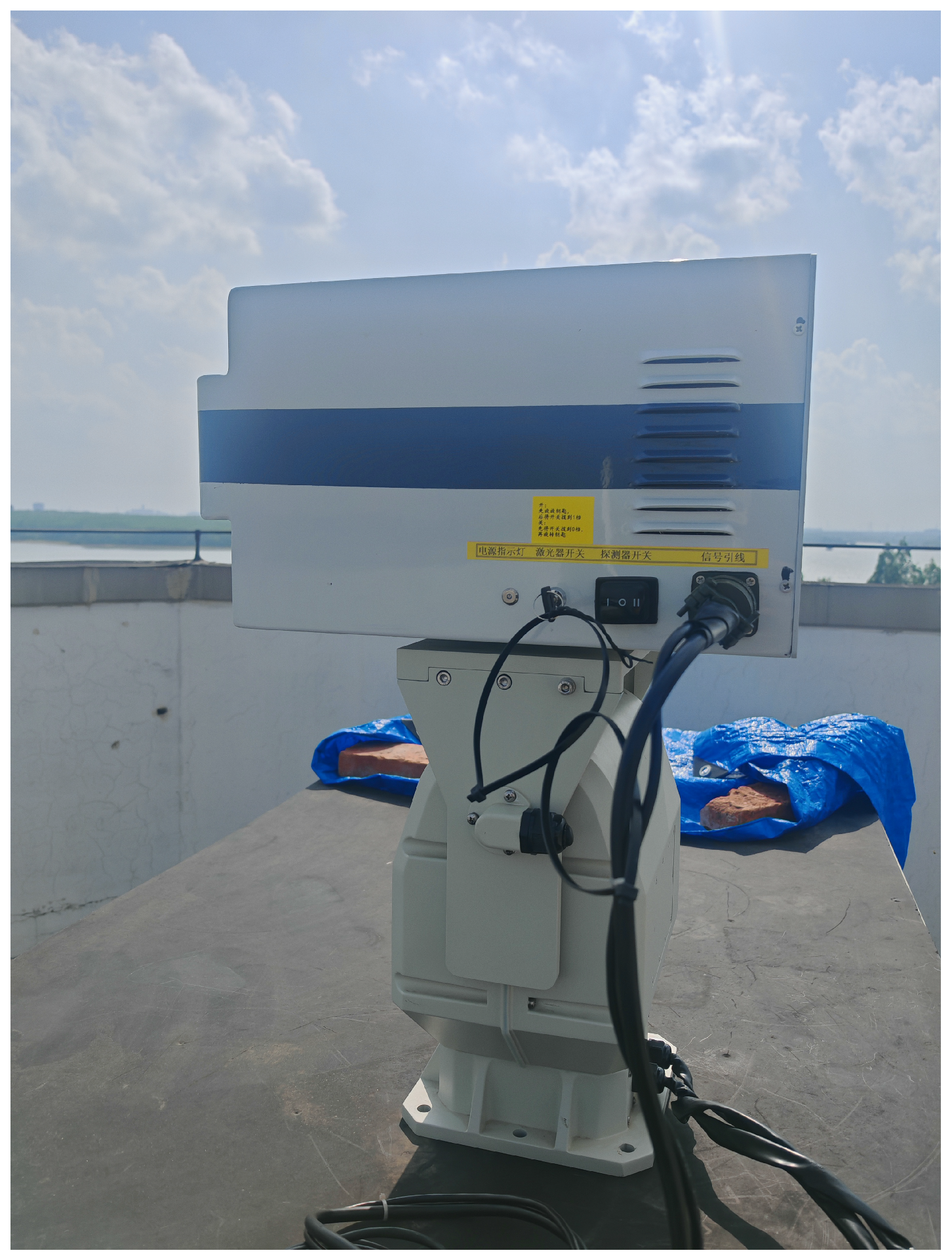
2.2. Instrumentation and Overview of the Data

In 2019, the WindPrint S4000 Coherent Doppler Wind Lidar (CDWL) developed by Qingdao Huahang Environmental Technology Co., Ltd. (Qingdao, China) was deployed at an observation site in the SCS for a year-long atmospheric wind field study. As illustrated in Figure 2, this lidar system operates in the infrared spectral region and features a vertical resolution of 30 m. It is capable of profiling atmospheric wind fields from the surface up to an altitude of 4000 m. The system continuously acquires a range of atmospheric parameters, including radial wind speed, horizontal wind speed, wind direction, vertical wind speed, signal-to-noise ratio (SNR), ground temperature, and atmospheric pressure. The specific parameters are provided in

Table 1. Technical parameters of the CDWL.

Technical Specification	Parameters
Wavelength	1550 nm
Pulse width	100–400 ns
Single-pulse energy	≥150 J
Radial detection range	0–75 m/s
Speed measurement accuracy	<±0.1 m/s
Radial detection range	50–6000 m

.

In November 2020, researchers from the Anhui Institute of Optics and Fine Mechanics (AIOFM) of the Chinese Academy of Sciences (CAS) conducted an experiment aboard CAS’s Survey Ship No. 1 to measure atmospheric optical turbulence. The oceanic $C_n^2$ was assessed using a radiosonde that ascended at approximately 6 m/s, offering a vertical resolution of about 10 m. The newly developed temperature pulsator had an average statistical time of 5 s and a frequency response range of 0.1–30 Hz. In this study, 12 valid radiosonde datasets were randomly selected; specific measurement records are detailed in

Table 2. Records of sounding details in the South China Sea.

Balloon Number	Experimental Date	Release Time (LT)	Terminal Time (LT)	Ultimate Altitude (m)
1	2020/10/17	15:56	17:30	15,620
2	2020/10/17	22:04	23:49	23,905
3	2020/10/18	18:29	20:16	30,968
4	2020/10/23	08:43	10:17	30,766
5	2020/10/25	08:52	10:32	31,702
6	2020/10/26	08:40	10:27	31,290
7	2020/11/02	19:23	21:33	31,690
8	2020/11/03	16:29	18:00	29,878
9	2020/11/04	16:53	18:34	28,797
10	2020/11/04	20:24	21:28	19,210
11	2020/11/12	16:27	17:59	30,030
12	2020/11/12	19:20	20:49	28,992

. The measurement principle of the $C_n^2$ radiosonde is detailed in Section 3.1.

Meteorological data near the surface were collected using the Vaisala WXT536 multi-parameter weather transmitter operating at a sampling frequency of 0.2 Hz. This compact and lightweight instrument simultaneously measures a suite of atmospheric variables, including barometric pressure (P), relative humidity (RH), precipitation, air temperature (T), average wind speed (WS), and wind direction (WD). The automated weather station (AWS) is engineered for consistent performance and is resilient to environmental challenges such as flooding, moisture loss, and evaporation.

The three-dimensional ultrasonic anemometer CSAT3 produced by Campbell Company was adopted in this study; the CSAT3 is a device used to measure three-dimensional wind speeds (u, v, w) and virtual temperature (Ts). As shown in Figure 3, it offers high temporal resolution and minimal inertia. In this experiment, the instrument was positioned at a height of 2 m with a sampling frequency of 20 Hz, providing accurate and timely wind speed data. Wang et al. [23] investigated the relationship between the similarity function of the temperature structure function and the temperature structure constant ($C_T^2$). Based on this relationship, we compared the new model with results from the CDWL study to further verify the model’s reliability.

As shown in Figure 4, the micro-pulse lidar (MPL) is designed to detect aerosol backscatter signals at a 532 nm wavelength, offering detection ranges of up to 5 km during daylight and extending to 15 km at night. With a temporal resolution of 5 min and a vertical resolution of 30 m, the MPL facilitates accurate atmospheric aerosol measurements. Its high detection capability and resolution have been documented [24]. In this study, MPL data are used to estimate the boundary layer height (BLH) in the SCS region by combining the raw signal gradient method with the threshold method.

Due to the absence of continuous, all-weather observational data for temperature and atmospheric pressure during the experimental period, this study utilizes ERA5 reanalysis data as a substitute. ERA5 is the fifth-generation global climate reanalysis dataset developed by the European Centre for Medium-Range Weather Forecasts (ECMWF) [25,26,27,28]. It comprises hourly data on atmospheric variables such as geopotential height, temperature, wind speed (including both horizontal components), and relative humidity, structured on a $0.{25}^{\circ }\times 0.{25}^{\circ }$ latitude–longitude grid. Additionally, ERA5 includes vertical profiles across 37 standard pressure levels. The ERA5 dataset is widely utilized in various fields, including weather forecasting, atmospheric research, climate change analysis, and prediction. While the CDWL can detect wind field information in real time, it cannot obtain temperature and pressure data simultaneously. To ensure the precise application of the ocean–atmosphere turbulence model to Doppler lidar in subsequent phases, in this study, ERA5 data are used instead of measured temperature and pressure data in combination with CDWL to calculate atmospheric turbulence parameters. The timing of ERA5 needs to be adjusted to the local time.

3. Principle of ${\mathit{C}}_{\mathit{n}}^{\mathit{2}}$ Measurement and Methods

3.1. Principle of $C_n^2$ Measurement

Under the assumption of Kolmogorov’s locally homogeneous and isotropic turbulence, the relationship between $C_n^2$, which characterizes the strength of atmospheric optical turbulence, and the atmospheric refractive index is as follows [1,29,30]:

$$C_n^2={\displaystyle \frac{〈{\left[n\left(\overrightarrow{x}\right)-n(\overrightarrow{x}+\overrightarrow{r})\right]}^2〉}{r^{2/3}}},l_0\ll r\ll L_0,$$

(1)

Here, $\langle ·\rangle$ denotes the ensemble average, n represents the refractive index of air, $\overrightarrow{x}$ and $\overrightarrow{r}$ denote positions in the atmosphere, and r is the magnitude of the separation vector. According to Kolmogorov’s theory, $l_0$ and $L_0$ are defined as the inner and outer scales of optical turbulence, respectively.

Similarly to $C_n^2$, $C_T^2$, the absolute humidity structure constant ($C_q^2$), and the temperature–humidity cross-structure constant ($C_{Tq}$) can be defined as follows:

$$C_T^2={\displaystyle \frac{〈{[T\left(\overrightarrow{x}\right)-T(\overrightarrow{x}+\overrightarrow{r})]}^2〉}{r^{2/3}}},l_0\ll r\ll L_0,$$

(2)

$$C_q^2={\displaystyle \frac{〈{[q\left(\overrightarrow{x}\right)-q(\overrightarrow{x}+\overrightarrow{r})]}^2〉}{r^{2/3}}},l_0\ll r\ll L_0,$$

(3)

$$C_{Tq}={\displaystyle \frac{〈[T\left(\overrightarrow{x}\right)-T(\overrightarrow{x}+\overrightarrow{r})][q\left(\overrightarrow{x}\right)-q(\overrightarrow{x}+\overrightarrow{r})]〉}{r^{2/3}}},l_0\ll r\ll L_0,$$

(4)

$C_n^2$ can be defined in terms of $C_T^2$, $C_q^2$, and $C_{Tq}$ as follows:

$$C_n^2=A^2{C}_T^2+2AB{C}_{Tq}+B^2{C}_q^2.$$

(5)

In atmospheric environments dominated by dry air, the influence of humidity on atmospheric optical turbulence can be neglected. In such cases, there is a direct relationship between $C_n^2$ and $C_T^2$. According to Equation (5), $C_n^2$ is related to the constants of the structure of the temperature, humidity, and temperature–humidity correlation. When the fluctuations in humidity are negligible, the effect on the refractive index structure constant can be ignored, and $C_n^2$ can be directly derived from $C_T^2$ [31,32]:

$$C_n^2={\left[79\times {10}^{-6}{\displaystyle \frac{P}{T^2}}\right]}^2{C}_T^2.$$

(6)

where P is the pressure in hPa; T is the temperature in K. As shown in Equation (2), $C_T^2$ can be obtained by averaging the squared temperature differences measured by two micro-temperature sensors separated by a known distance.

3.2. Tatarski Model

The Tatarski outer-scale model represents a classical approach to turbulence estimation, primarily based on fundamental turbulence theory. It establishes a relationship between conventional meteorological parameter profiles and $C_n^2$ profiles via the outer-scale model. According to Kolmogorov’s local homogeneous isotropic turbulence theory, Tatarski expresses $C_n^2$ as follows [1]:

It is worth noting that in this study, small-scale turbulence is assumed to be isotropic. Although some studies have suggested that significant anisotropy may still exist at small scales [33], this is not within the scope of discussion in this article at present.

$$C_n^2=a^2{L}_0^{4/3}{M}^2,$$

(7)

In this context, $a^2$ denotes a constant, usually set to 2.8, $L_0$ is the outer scale, and M signifies the potential refractive index gradient. This gradient is derived from potential temperature, temperature, and pressure according to the following equation:

$$M=-{\displaystyle \frac{79\times {10}^{-6}P}{T^2}}\times {\displaystyle \frac{d\theta }{dh}},$$

(8)

$$\theta =T{\left({\displaystyle \frac{1000}{P}}\right)}^{0.286},$$

(9)

Dewan et al. derived the Dewan model from extensive experimental observations, emphasizing its association with wind shear. The model is expressed as follows [34]:

$$S=\sqrt{({\displaystyle \frac{\partial u}{\partial h}}{)}^2+({\displaystyle \frac{\partial v}{\partial h}}{)}^2},$$

(10)

where the variables u and v represent the zonal and meridional wind components, respectively.

$${L_0}^{4/3}=\left\{\begin{array}{c}{0.1}^{4/3}\times {10}^{1.64+42\times S},\mathrm{troposphere}\hfill \\ {0.1}^{4/3}\times {10}^{0.506+50\times S},\mathrm{stratosphere}\hfill \end{array}.\right.$$

(11)

In 2002, Jackson and Reynolds developed the HMNSP99 outer-scale model based on extensive experimental sounding data. This model incorporates both wind shear and temperature gradient, and it is expressed as follows [35]:

$${L_0}^{4/3}=\left\{\begin{array}{c}{0.1}^{4/3}\times {10}^{0.362+16.728\times S-192.347\times {\displaystyle \frac{dT}{dh}}},\mathrm{troposphere}\hfill \\ {0.1}^{4/3}\times {10}^{0.757+13.819\times S-57.784\times {\displaystyle \frac{dT}{dh}}},\mathrm{stratosphere}\hfill \end{array}.\right.$$

(12)

3.3. Estimating Atmospheric Turbulence Parameters

Turbulence intensity (I) reflects the fluctuation intensity of the wind, where the variance is defined as follows:

$${\sigma }_A^2={\displaystyle \frac{1}{N}}\sum _{i=0}^{N-1}{(A_i-\overline{A})}^2=\overline{a^{\prime 2}},$$

(13)

where ${\sigma }_A$ is the standard deviation. The standard deviations of the three components of wind speed are ${\sigma }_u={\overline{(u^{\prime 2}})}^{1/2}$, ${\sigma }_v={\overline{(v^{\prime 2}})}^{1/2}$, and ${\sigma }_w={\overline{(w^{\prime 2}})}^{1/2}$. Their ratio to the horizontal wind speed modulus $\overline{u}$ is called the turbulence intensity. The turbulence intensity of the wind speed in the x, y, and z directions is as follows:

$$I_x={\displaystyle \frac{{\sigma }_u}{u}},$$

(14)

$$I_y={\displaystyle \frac{{\sigma }_v}{u}},$$

(15)

$$I_z={\displaystyle \frac{{\sigma }_w}{u}}.$$

(16)

Turbulent kinetic energy (TKE) measures turbulence intensity and plays a crucial role in the transport of atmospheric momentum, heat, and water vapor in the boundary layer. It is defined as follows [36]:

$$TKE={\displaystyle \frac{1}{2}}\left({\sigma }_u^2+{\sigma }_v^2+{\sigma }_w^2\right).$$

(17)

3.4. Estimation of Near-Surface $C_n^2$ Based on CSAT3

By applying a series of preprocessing techniques—including outlier removal, virtual temperature correction, and coordinate rotation—to the original data from the CSAT3 and WXT536 instruments, we obtained three-dimensional wind velocity components, temperature, atmospheric pressure, and other relevant parameters. Subsequently, using Monin–Obukhov Similarity Theory (MOST) and dimensional analysis, we calculated $C_n^2$. The calculation method for $\zeta$ is as follows [37,38,39,40]:

$$\zeta ={\displaystyle \frac{z}{L}},$$

(18)

$$L=-{\displaystyle \frac{\rho u_{*}^2}{kg\left(\frac{H}{c_p{T}_a}\right)}},$$

(19)

$$H=\rho c_p\left(w^{\prime }{T}^{\prime }\right),$$

(20)

$$u_{*}={\left({\overline{u^{\prime }{w}^{\prime }}}^2+{\overline{v^{\prime }{w}^{\prime }}}^2\right)}^{1/4},$$

(21)

Here, L is the Obukhov length, H is the sensible heat flux, $u_{*}$ is the friction velocity, z is the height, $\rho$ is the air density, k is the von Kármán constant, g is gravitational acceleration, $c_p$ is the specific heat at constant pressure, and $T_a$ is the air temperature. The friction velocity and Obukhov length can be calculated by measuring the fluctuations of the three-dimensional wind components ($u^{\prime }$, $v^{\prime }$, $w^{\prime }$) and temperature fluctuation ($T^{\prime }$).

Wang et al. [23] analyzed the measured data from the SCS, and, based on previously proposed similarity functions under both unstable and stable conditions, identified a similarity function for the temperature structure constant in the offshore layer of the SCS. The resulting formula is as follows:

$$g\left(\zeta \right)=\left\{\begin{array}{c}0.85,\zeta \le -1,\hfill \\ 15.7{\left(1-79.5\zeta \right)}^{-2/3},-1<\zeta \le 0\hfill \\ 15.7{\left(1+382.3\zeta \right)}^{-2/3},\zeta >0\hfill \end{array}\right.,$$

(22)

$$g\left(\zeta \right)={\displaystyle \frac{C_T^2{z}^{2/3}}{T_{*}^2}},$$

(23)

$$T_{*}={\displaystyle \frac{\overline{w^{\prime }{T}^{\prime }}}{u_{*}}}.$$

(24)

Finally, the relationship between $g\left(\zeta \right)$ and $C_T^2$ is employed to derive the daily variation characteristics of near-surface $C_n^2$ in the SCS. This method aids in verifying the turbulent characteristics of the atmospheric boundary layer, providing important references for related meteorological studies.

4. Results and Discussion

4.1. New Statistical Model of the Marine Atmospheric Boundary Layer

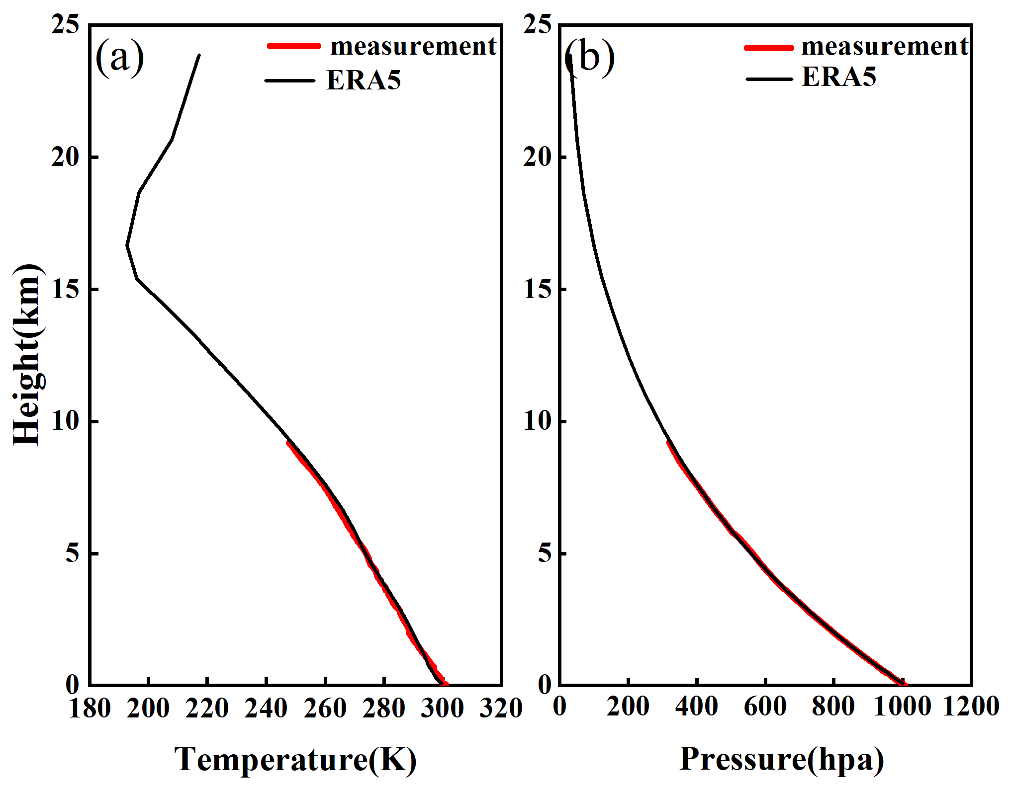
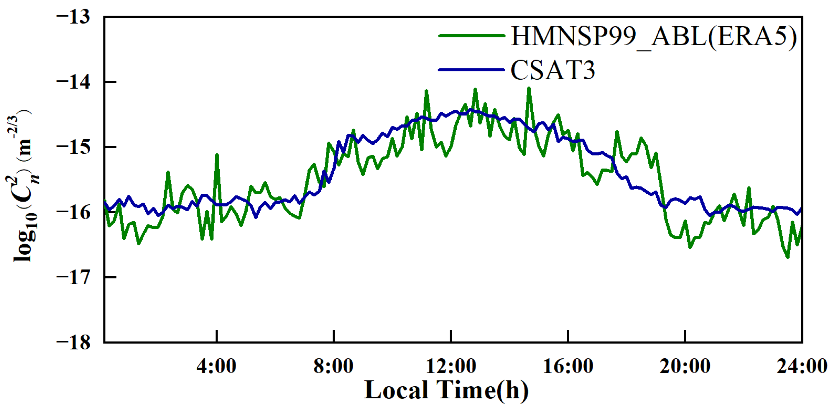
In contrast to Dewan’s outer-scale model [34], the HMNSP99 model [35] incorporates temperature gradient considerations. Although temperature variations in the atmospheric boundary layer are not always pronounced, prior research indicates that both temperature gradients and wind shear significantly influence atmospheric optical turbulence. Consequently, the HMNSP99 model was selected to estimate atmospheric optical turbulence parameters. Utilizing sonde experiment data obtained from the ship, parameters such as altitude, wind speed, and wind direction were retrieved. However, since CDWL cannot detect temperature and pressure profiles in real time, temperature and pressure profiles from the ERA5 dataset were employed as substitutes for sonde measurements, ensuring accurate model application to CDWL in subsequent phases.

Figure 5 presents a comparison of the mean temperature and pressure profiles derived from ERA5 reanalysis data and in situ measurements from the radiosonde. The results show that the trends between the two datasets are consistent and the deviation is small.

Figure 6 illustrates the distribution of temperature and pressure data points from ERA5 and radiosonde measurements during the observation period; the correlation coefficient (R) reaches 0.99. This further confirms that ERA5 reanalysis data can serve as a reliable alternative for temperature and pressure information in the absence of direct measurements.

As depicted in Figure 7, the aerosol extinction coefficient was extracted through the analysis of MPL echo signals. The BLH was subsequently determined with high accuracy by integrating the threshold method and the gradient method [24]. The blank stripes in Figure 7 are mainly caused by data quality control measures applied during the processing of raw signals from the MPL. Although these stripes indicate localized data gaps, they do not affect the overall determination of the BLH. The results further demonstrate that the ABL height in the SCS remains at approximately 2 km throughout the day, exhibiting minimal diurnal variation. This suggests that the near-surface layer in this region is likely confined to a thickness range of 100 to 200 m.

The near-surface layer, constituting the lowest segment of the ABL, is directly influenced by surface friction and thermal effects, leading to rapid variations in meteorological parameters such as wind speed and temperature with increasing altitude. The thickness of this layer is determined by a combination of surface characteristics, topographical features, and atmospheric stability, all of which significantly impact the turbulence structure and flow dynamics within the ABL [23,41,42].

Observations over the SCS reveal that $C_n^2$ exhibits an exponential decay with height in the near-surface layer, indicating a swift attenuation of turbulence intensity close to the surface. Above this layer, the rate of turbulence decrease becomes more gradual, reflecting a smoother vertical variation. The HMNSP99 model (Equation (12)) fails to accurately describe the variation in near-surface turbulence with height. Therefore, based on $C_n^2$ sounding profiles, the HMNSP99 model was improved for the near-surface layer and the boundary layer. This improved model is referred to as HMNSP99_ABL (ERA5), and its results are as follows:

$${L_0}^{4/3}=\left\{\begin{array}{cc}{0.1}^{4/3}\times {10}^{0.032+88.728\times S-111.525{\displaystyle \frac{dT}{dh}}},\hfill & \hfill 0<z\le 150\\ {0.1}^{4/3}\times {10}^{0.138+92.648\times S-128.258{\displaystyle \frac{dT}{dh}}},\hfill & \hfill 150<z\le 2000\end{array}\right..$$

(25)

As shown in Figure 8, to further elucidate the process of $C_n^2$ estimation, which relies on ERA5-derived temperature and pressure data combined with wind speed measurements from CDWL, a detailed flowchart is depicted. The figure demonstrates the sequential fitting of ERA5 temperature and pressure data with radiosonde wind speed measurements; the fitted result yields Equation (25). This is followed by the incorporation of CDWL wind speed data for refined analysis and processing. This integrated approach facilitates a more precise estimation of atmospheric optical turbulence parameters, contributing valuable insights for meteorological research and forecasting applications.

As shown in Figure 9a, there is a strong agreement between the new model and the measured results. The solid red line represents the mean value of the radiosonde experiment data, while the solid black line denotes the predicted results of the HMNSP99_ABL (ERA5) model, demonstrating consistency in both trend and order of magnitude. The absolute deviation between the two remains within one order of magnitude, and the correlation coefficient $R_{xy}$ exceeds 0.85, further confirming their high correlation. The green solid line represents the estimation result of the external scale model of HMNSP99 (Equation (12)); compared with the observational data, the model inadequately captures the vertical variation in near-surface turbulence.

Figure 9c presents the scatterplot distribution of the HMNSP99_ABL (ERA5) model estimates against the turbulent meteorosonde measurements. The observed results indicate that the measured values are symmetrically distributed around the $y=x$ line, suggesting that the outer-scale model provides an accurate estimation of atmospheric turbulence characteristics within the marine atmospheric boundary layer (MABL).

In this study, the measured three-dimensional wind speed, temperature, and potential temperature data were used to calculate the turbulence characteristic parameters $u_{*}$, $T_{*}$, and $g\left(\zeta \right)$ using Equations (18)–(24), thereby obtaining the near-surface variation trend of $C_n^2$.

To evaluate the accuracy of the HMNSP99_ABL(ERA5) model in estimating $C_n^2$ within the atmospheric boundary layer (ABL), the diurnal variation in $C_n^2$ at a height of 52 m was analyzed using the aforementioned method; this was achieved by integrating the measurement data (including surface wind speed and wind direction) with the newly developed similarity functions. The results were then compared with the predictions from the HMNSP99_ABL (ERA5) model. The detailed comparison is shown in Figure 10.

To further evaluate the applicability and accuracy of the new model in the near-surface layer, the diurnal variation in $C_n^2$ estimated by the model was compared with near-surface layer data, as shown in Figure 10. The green curve represents the $C_n^2$ values calculated using the new model based on CDWL data at the lowest level (52 m). The blue curve shows the results derived from the ultrasonic anemometer measurements (see Section 3.4), where the observed $C_n^2$ at 2 m height was normalized to the model’s lowest level (52 m) using the surface layer similarity theory (Equations (18)–(24)). The results indicate a strong agreement between the two in terms of both trend and magnitude.

4.2. Error Analysis

In order to analyze the reliability of the HMNSP99_ABL (ERA5) model in greater depth, we employed a range of quantitative and qualitative metrics, including correlation coefficient ($R_{xy}$), mean relative error (MRE), root mean square error (RMSE), and bias (Bias), to assess the correlation between the measured and estimated values in the sounding data [43,44]. The corresponding expressions are as follows:

$$R_{xy}={\displaystyle \frac{{\displaystyle \sum _{i=1}^N}\left(X_i-\overline{X}\right){\displaystyle \sum _{i=1}^N}\left(Y_i-\overline{Y}\right)}{\sqrt{{\displaystyle \sum _{i=1}^N}{\left(X_i-\overline{X}\right)}^2{\displaystyle \sum _{i=1}^N}{\left(Y_i-\overline{Y}\right)}^2}}},$$

(26)

$$MRE={\displaystyle \frac{1}{N}}\sum _{i=1}^N|X_i-Y_i|,$$

(27)

$$RMSE=\sqrt{\sum _{i=1}^N{\displaystyle \frac{{\left(X_i-Y_i\right)}^2}{N}}},$$

(28)

$$Bias={\displaystyle \frac{1}{N}}\sum _{i=1}^N(X_i-Y_i).$$

(29)

In the aforementioned description, $X_i$ represents the measured values from the soundings, $Y_i$ denotes the $C_n^2$ values estimated by the HMNSP99_ABL (ERA5) model, and N represents the total number of samples, i.e., the number of $(X_i,Y_i)$ data pairs. The statistical analysis of the error between the measured and estimated values for an individual sounding is presented in Figure 10.

The HMNSP99_ABL (ERA5) model was employed to estimate the $C_n^2$ profile for 12 soundings. The discrepancies between the estimated $C_n^2$ profiles and the corresponding measured $C_n^2$ profiles were analyzed using the specified formulas for error statistics. The detailed statistical results are provided in the following.

As shown in Figure 11, the changes in MRE, RMSE, and Bias between each detection experiment and the HMNSP99_ABL (ERA5) model can be observed. The bias values exhibit a relatively narrow range, centered between $-0.5$ and $0.5$, while the RMSE and MRE generally remain below 1. This indicates that, although certain errors may arise under specific weather conditions, using temperature and pressure profiles from the ERA5 to replace radiosonde observations in combination with a stratified modeling approach remains a reliable method for studying turbulence models applicable to marine environments.

As shown in

Table 3. Statistical analysis of the estimation of $C_n^2$ in the SCS region using the HMNSP99_ABL (ERA5) model.

${\mathbf{R}}_{\mathit{xy}}$	RMSE	MRE	Bias
0.67	0.92	0.59	0.08

, the error profiles of the 12 radiosonde datasets are averaged. It is observed that the overall correlation coefficient $R_{xy}$ is 0.67, exceeding the threshold of 0.6 [36,43,44,45]. This suggests that the HMNSP99_ABL (ERA5) model can reasonably capture the variations in optical turbulence within the ABL.

Compared with conventional observational methods, CDWL offers significant advantages, including all-sky coverage and a high spatiotemporal resolution. Furthermore, its high detection accuracy (≤0.1 m/s) and rapid data update rate (1 s) facilitate a more detailed investigation into the vertical structure and spatiotemporal evolution of turbulence parameters in the ABL.

To evaluate the reliability of estimating $C_n^2$ using high-precision CDWL wind speed measurements, an analysis was conducted to assess the impact of detection accuracy on $C_n^2$ estimation. This investigation was carried out using Equations (7)–(10) and (25).

$$C_n^2=1.75\times {10}^{-8}\times L_0^{{\displaystyle \frac{4}{3}}}\times P^2\times {\left({\displaystyle \frac{d\theta }{dh}}\right)}^2\times T^{-4},$$

(30)

$${\displaystyle \frac{\partial C_n^2}{\partial S}}=1.7\times {10}^{-7}\times P^2\times {\left({\displaystyle \frac{d\theta }{dh}}\right)}^2\times {10}^{0.032+88.728\times S-111.525\times {\displaystyle \frac{dT}{dh}}}\times T^{-4},$$

(31)

Based on the measured data, $P=854$, $S=0.0046$, $T=290$, ${\displaystyle \frac{dT}{dh}}=0.005$, and ${\displaystyle \frac{d\theta }{dh}}=0.0049$.

$$▵C_n^2\approx {\displaystyle \frac{\partial C_n^2}{\partial S}}\times ▵S\approx 2.8\times {10}^{-17}.$$

(32)

To assess the reliability of estimating the refractive index structure constant $C_n^2$ using high-precision CDWL wind speed data, this study conducted a partial derivative analysis of Equations (30) and (31) to investigate the impact of measurement errors on the $C_n^2$ results. Calculations based on actual observational data indicate that the magnitude of the error term on the results is only $2.8\times {10}^{-17}$, which can be considered negligible. This suggests that, even with some measurement uncertainties, CDWL data still exhibit good stability and reliability in estimating $C_n^2$, providing a solid data foundation for subsequent atmospheric optical turbulence studies.

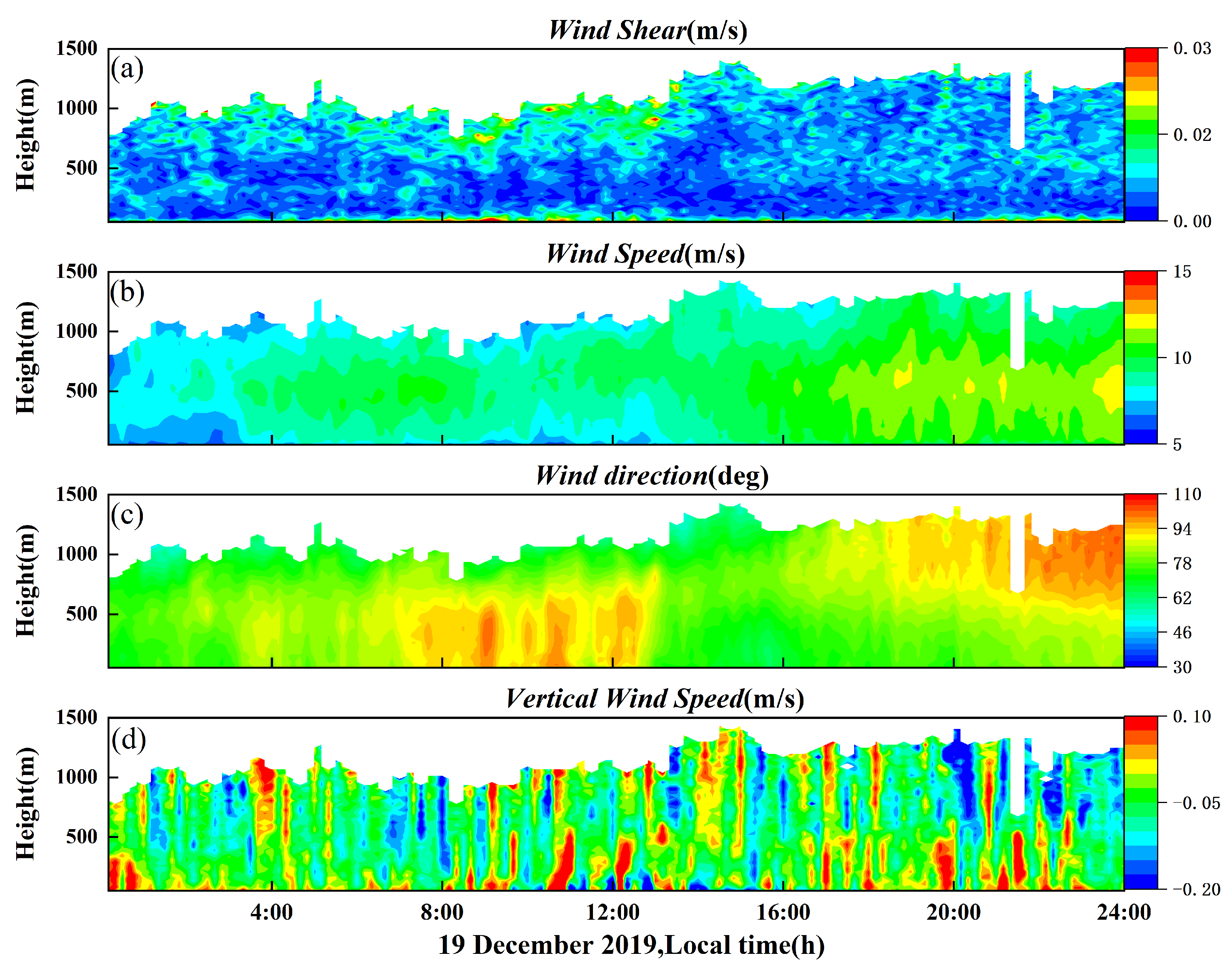
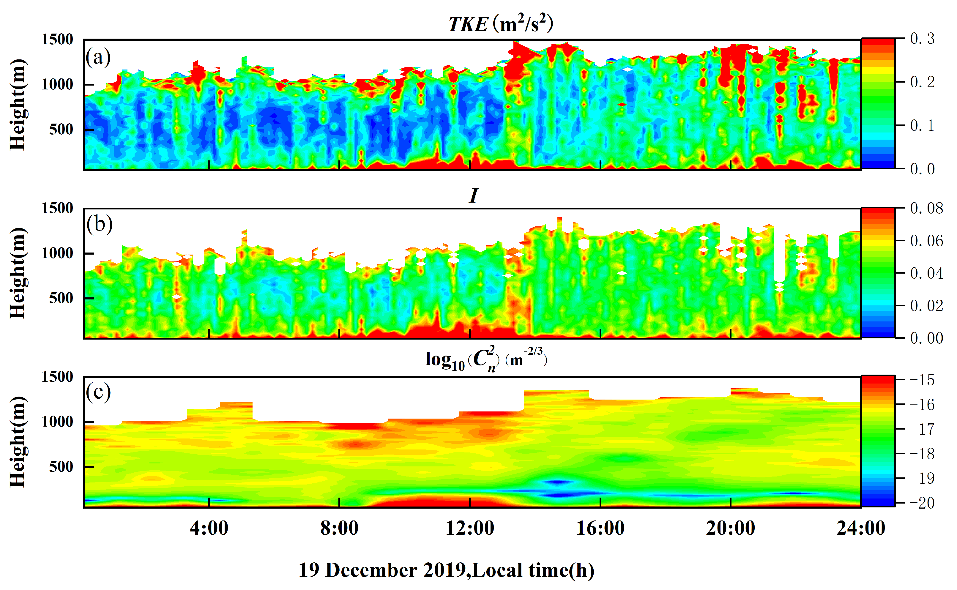
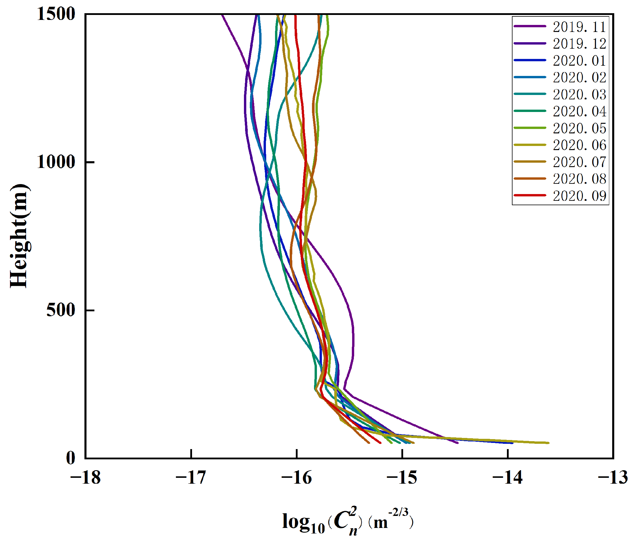
4.3. Characteristics of Turbulent Parameters in the MABL by Combining CDWL and HMNSP99_ABL (ERA5) Models

A comprehensive understanding of the characteristics of variations in optical turbulence parameters—including wind speed, wind direction, $C_n^2$, I, $TKE$, and others—is crucial for developing continuous time-series estimation methods for optical turbulence parameters in the MABL. This study employs the CDWL and HMNSP99_ABL (ERA5) models to analyze the characteristics of turbulent parameters in the MABL.

The above experiments verified the validity of the method used by the new model to estimate $C_n^2$. Here, measured wind speed and direction are integrated with ERA5 reanalysis data for temperature and pressure. Consequently, real-time wind profile data obtained from the CDWL are combined with ERA5 temperature and pressure data from the corresponding days to derive the spatiotemporal distribution of $C_n^2$ throughout the entire day.

As shown in Figure 12, CDWL data from a randomly selected sample day are used, and the described method is applied to extract five distinct levels from the estimated $C_n^2$ data, enabling the derivation of characteristic daily variation curves for these levels. Within the ABL, $C_n^2$ gradually decreases with altitude and exhibits clear diurnal variations, aligning with prior research findings [22]. Moreover, the curves demonstrate a “Mexican hat” shape to varying degrees [46], with this feature weakening as the altitude increases. Over the course of the day, $C_n^2$ typically increases and reaches its peak between 09:00 and 13:00 local time, before beginning to decline. The evolution of optical turbulence in the ABL is closely tied to temperature and wind shear. This phenomenon may be due to the large volume and high heat capacity of seawater, which causes the sea surface temperature to change slowly, thereby reducing the influence of solar radiation on the diurnal cycle of turbulence.

In order to gain a deeper insight into the diurnal variation in atmospheric turbulence parameters, we computed the continuous results of the CDWL measurements. Figure 13 presents the key wind parameters measured with the CDWL, including the horizontal wind speed, horizontal wind direction, wind shear, and vertical wind speed. The horizontal wind speed fluctuates between approximately 5 m/s and 15 m/s, while the vertical wind speed ranges from −0.2 m/s to 0.1 m/s. Additionally, a significant shift in wind direction is observed between 08:00 and 12:00. The distribution of horizontal and vertical wind speeds is relatively uniform overall, potentially due to the generally flat topography of the sea, which facilitates uniform wind propagation across the sea surface and minimal variation in wind speed. Furthermore, wind blowing over the sea surface gives rise to local disturbances that interact with sea surface friction, particularly in the area of wave formation. Such disturbances can exert an influence on wind speed, resulting in relatively insignificant alterations in wind speed.

Based on Equations (14) and (17) in Section 3.3, the spatiotemporal distributions of $C_n^2$, TKE, and I were obtained. Figure 14 illustrates that the overall diurnal variation characteristics of $C_n^2$ in the ABL of the SCS are relatively insignificant [47], whereas the diurnal variation characteristics near the surface are more pronounced. The development of atmospheric optical turbulence is correlated with factors such as wind shear and temperature, as illustrated in the figure. At the sea surface, minor fluctuations in wind speed result in diminished wind shear. The formation of atmospheric turbulence is significantly influenced by wind shear. The presence of weak wind shear will serve to restrict the development and diffusion of turbulence, thereby ensuring a relatively stable atmospheric environment. Additionally, minor temperature discrepancies can influence the magnitude of turbulent activity. It can thus be surmised that these factors may exert an influence on the diurnal characteristics of turbulence.

The magnitude and spatial distribution of TKE are essential for describing the characteristics, propagation, and evolution of atmospheric turbulence. The study of turbulent kinetic energy is particularly relevant to meteorology, climate science, and air quality research. As illustrated in Figure 13, the trends in TKE and I closely align with those of turbulence intensity $C_n^2$. Near the surface, TKE and I exhibit larger values, increasing gradually over time. Notably, turbulence intensity peaks around noon, likely due to the effects of solar radiation. At around 12:00, when solar radiation is at its strongest, the boundary layer becomes most active, subsequently weakening at night. However, local meteorological conditions can also influence these patterns.

To achieve a more comprehensive understanding of the characteristics of atmospheric optical turbulence over the SCS, we utilized the HMNSP99_ABL (ERA5) model alongside the measured CDWL data and temperature and pressure data from ERA5. This approach enabled us to investigate the turbulence intensity $C_n^2$ within the atmospheric boundary layer over the SCS from November 2019 to September 2020.

As illustrated in Figure 15, the monthly mean median profile distribution of $C_n^2$ in the atmospheric boundary layer of the SCS is presented. The $C_n^2$ profile exhibits a gradual decline with increasing altitude, with its mean values predominantly ranging between ${10}^{-17}$ and ${10}^{-15}{\mathrm{m}}^{-2/3}$. In addition, the monthly mean profiles of $C_n^2$ over the 11-month period exhibit relatively small differences in vertical structure.

A stratified analysis of the statistical characteristics of the optical turbulence structure parameter $C_n^2$ across different height ranges (52–500 m, 500–1000 m, and 1000–1500 m) is presented in Figure 15. As shown in Figure 16, the overall turbulence intensity decreases with increasing altitude; however, the distribution characteristics differ significantly across the layers. In the 52–500 m range (Figure 16a), the $C_n^2$ values are relatively concentrated and exhibit a near-unimodal distribution. In the 500–1000 m layer (Figure 16b), the distribution shifts slightly and the peak value decreases, indicating a weakening of turbulence intensity in the mid-layer. In the 1000–1500 m layer (Figure 16c), the distribution becomes noticeably broader, suggesting that turbulence activity at this height is influenced by more complex atmospheric processes, such as upper-level inflows, inversion layers, and advective transport, leading to increased variability.

5. Summary

In this study, based on the variation in $C_n^2$ within the atmospheric boundary layer over the SCS derived from radiosonde data, we developed a new atmospheric boundary layer model for the region, building upon the HMNSP99 outer-scale model. This was achieved by integrating radiosonde observations with ERA5 reanalysis data and subsequently applying the refined model to CDWL to estimate $C_n^2$. Based on Monin–Obukhov Similarity Theory (MOST) and ultrasonic anemometer observations, we compared the new model with near-surface $C_n^2$, and the results showed that the two had a strong correlation, thereby validating the reliability of the HMNSP99_ABL (ERA5) model from multiple perspectives. This study lays the groundwork for utilizing CDWL for estimating atmospheric turbulence parameters.

A comparative analysis of ERA5 temperature and pressure data with simultaneous radiosonde observations reveals a strong correlation, confirming that ERA5 data can effectively substitute real-time measurements when direct temperature and pressure profiles are unavailable. By integrating CDWL measured wind speed, wind direction, and turbulence parameters—such as $C_n^2$, TKE, and I—this study provides a more comprehensive insight into the evolution of atmospheric turbulence within the ABL over the ocean.

The findings indicate that the spatial and temporal variations in optical turbulence parameters in the SCS are relatively insignificant within the ABL, but exhibit pronounced diurnal patterns near the surface. This phenomenon can be primarily attributed to the substantial heat capacity of seawater, which moderates temperature fluctuations by absorbing and releasing heat energy, thereby maintaining a stable sea surface temperature. The thermal inertia of seawater prevents rapid temperature shifts due to solar radiation, consequently suppressing turbulence generation. Furthermore, the higher density of seawater compared with that of air results in a slower rate of heat exchange, further diminishing the diurnal characteristics of turbulence.

The results indicate that the monthly statistical characteristics of $C_n^2$ in the atmospheric boundary layer over the SCS are generally stable and exhibit a decreasing trend with altitude. However, the applicability of the outer-scale model may be limited by insufficient observational data and the impact of sporadic extreme weather events. Nevertheless, this remains a useful framework for exploring optical turbulence in coastal regions. Additionally, in scenarios where direct temperature and pressure measurements are unavailable, ERA5 data serve as a practical and reliable substitute. Given the dynamic nature of marine environments, acquiring diverse and continuous observational datasets is essential for constructing accurate optical turbulence models. This will further contribute to the enhancement of photoelectric system stability and optimization, ensuring improved performance in real-world applications.

References

1. Tatarski, V.I. Wave Propagation in a Turbulent Medium; McGraw-Hill: New York, NY, USA, 1961; Volume 14, 285p. [Google Scholar] [CrossRef]
2. Good, R.E.; Beland, R.R.; Murphy, E.A.; Brown, J.H.; Dewan, E.M. Atmospheric Models Of Optical Turbulence. Proc. SPIE 1988, 928, 165–186. [Google Scholar]
3. Ata, Y.; Baykal, Y.; Gke, M.C. Average channel capacity in anisotropic atmospheric non-Kolmogorov turbulent medium. Opt. Commun. 2019, 451, 129–135. [Google Scholar] [CrossRef]
4. Kim, S.H.; Chun, H.Y.; Lee, D.B.; Kim, J.H.; Sharman, R.D. Improving Numerical Weather Prediction-Based Near-Cloud Aviation Turbulence Forecasts by Diagnosing Convective Gravity Wave Breaking. Weather Forecast. 2021, 36, 1735–1757. [Google Scholar] [CrossRef]
5. Ren, Y.; Zhang, H.S.; Wei, W.; Wu, B.G.; Cai, X.H.; Song, Y. Effects of turbulence structure and urbanization on the heavy haze pollution process. Atmos. Chem. Phys. 2019, 19, 1041–1057. [Google Scholar] [CrossRef]
6. Ren, Y.; Zhang, H.S.; Wei, W.; Cai, X.H.; Song, Y.; Kang, L. A study on atmospheric turbulence structure and intermittency during heavy haze pollution in the Beijing area. Sci. China Earth Sci. 2019, 62, 2058–2068. [Google Scholar] [CrossRef]
7. Zhang, Q.; Zhang, J.; Qiao, J.; Wang, S. Relationship of atmospheric boundary layer depth with thermodynamic processes at the land surface in arid regions of China. Sci. China Earth Sci. 2011, 54, 1586–1594. [Google Scholar] [CrossRef]
8. Bi, C.C.; Qing, C.; Wu, P.F.; Jin, X.M.; Liu, Q.; Qian, X.M.; Zhu, W.Y.; Weng, N.Q. Optical Turbulence Profile in Marine Environment with Artificial Neural Network Model. Remote Sens. 2022, 14, 2267. [Google Scholar] [CrossRef]
9. Eaton, F.D. Recent developments of optical turbulence measurement techniques (Invited Paper). Proc. SPIE 2005, 5793. [Google Scholar]
10. Shelekhov, A.; Afanasiev, A.; Shelekhova, E.; Kobzev, A.; Tel’minov, A.; Molchunov, A.; Poplevina, O. High-Resolution Profiling of Atmospheric Turbulence Using UAV Autopilot Data. Drones 2023, 7, 412. [Google Scholar] [CrossRef]
11. Qian, X.; Yao, Y.Q.; Zou, L.; Wang, H.S.; Li, J.W. Optical turbulence in the atmospheric surface layer at the Ali Observatory, Tibet. Mon. Not. R. Astron. Soc. 2022, 510, 5179–5186. [Google Scholar] [CrossRef]
12. Hufnagel, R.E.; Stanley, N.R. Modulation transfer function associated with image transmission through turbulent media. J. Opt. Soc. Am. 1964, 54, 52. [Google Scholar] [CrossRef]
13. Thorpe, S.A. Turbulence and Mixing in a Scottish Loch. Philos. Trans. R. Soc. A 1977, 286. [Google Scholar]
14. Banakh, V.A.; Smalikho, I.N.; Falits, A.V.; Sherstobitov, A.M. Estimating the Parameters of Wind Turbulence from Spectra of Radial Velocity Measured by a Pulsed Doppler Lidar. Remote Sens. 2021, 13, 2071. [Google Scholar] [CrossRef]
15. Smalikho, I.N.; Banakh, V.A. Effect of Wind Transport of Turbulent Inhomogeneities on Estimation of the Turbulence Energy Dissipation Rate from Measurements by a Conically Scanning Coherent Doppler Lidar. Remote Sens. 2020, 12, 2802. [Google Scholar] [CrossRef]
16. Yuan, J.; Xia, H.; Wei, T.; Wang, L.; Wu, Y. Identifying cloud, precipitation, windshear, and turbulence by deep analysis of the power spectrum of coherent Doppler wind lidar. Opt. Express 2020, 28, 37406. [Google Scholar] [CrossRef]
17. Wang, C.; Jia, M.J.; Xia, H.Y.; Wu, Y.B.; Wei, T.W.; Shang, X.; Yang, C.Y.; Xue, X.H.; Dou, X.K. Relationship analysis of PM2.5 and boundary layer height using an aerosol and turbulence detection lidar. Atmos. Meas. Tech. 2019, 12, 3303–3315. [Google Scholar] [CrossRef]
18. Zhang, H.J.; Zhu, L.M.; Sun, G.; Zhang, K.; Xu, M.M.; Liu, N.A.; Chen, D.L.; Wu, Y.; Cui, S.C.; Luo, T.; et al. Estimation and characterization of the refractive index structure constant within the marine atmospheric boundary layer. Appl. Opt. 2022, 61, 9762–9772. [Google Scholar] [CrossRef]
19. Zhu, L.; Sun, G.; Zhang, H.; Xu, M.; Chen, D.; Shao, S.; Wu, P.; Li, X. Study on High Resolution Optical Turbulence Estimation Model of Marine Atmospheric Boundary Layer Using Lidar. Acta Opt. Sin. 2022, 42, 1201004. [Google Scholar]
20. Jiang, P.; Yuan, J.L.; Wu, K.N.; Wang, L.; Xia, H.Y. Turbulence Detection in the Atmospheric Boundary Layer Using Coherent Doppler Wind Lidar and Microwave Radiometer. Remote Sens. 2022, 14, 2951. [Google Scholar] [CrossRef]
21. Qing, H.Y.; Zhang, Y.N.; Zhou, C.; Zhao, Z.Y.; Chen, G. Atmospheric temperature profiles estimated by the vertical wind speed observed by MST radar. Acta Phys. Sin. 2014, 63, 094301. [Google Scholar] [CrossRef]
22. Xu, M.M.; Zhou, L.P.; Shao, S.Y.; Weng, N.Q.; Liu, Q. Analyzing the Effects of a Basin on Atmospheric Environment Relevant to Optical Turbulence. Photonics 2022, 9, 235. [Google Scholar] [CrossRef]
23. Wang, F.; Zhang, K.; Sun, G.; Liu, Q.; Li, X.; Luo, T. Study of the C n 2 Model through the New Dimensionless Temperature Structure Function near the Sea Surface in the South China Sea. Remote Sens. 2023, 15, 631. [Google Scholar] [CrossRef]
24. Liu, N.; Luo, T.; Han, Y.; Yang, K.; Wu, Y.; Zhang, K.; Weng, N.; Li, X. Influence of Typhoon Peripheral Circulation on the Atmospheric Boundary Layer Structure in Coastal Areas. Acta Opt. Sin. 2021, 41, 041. [Google Scholar]
25. Kuo, C.L. Assessments of Ali, Dome A, and Summit Camp for mm-wave Observations Using MERRA-2 Reanalysis. Astrophys. J. 2017, 848, 64. [Google Scholar] [CrossRef]
26. Kobayashi, S.; Ota, Y.; Harada, Y.; Ebita, A.; Moriya, M.; Onoda, H.; Onogi, K.; Kamahori, H.; Kobayashi, C.; Endo, H.; et al. The JRA-55 Reanalysis: General Specifications and Basic Characteristics. J. Meteorol. Soc. Jpn. 2015, 93, 5–48. [Google Scholar] [CrossRef]
27. Saha, S.; Moorthi, S.; Wu, X.R.; Wang, J.; Nadiga, S.; Tripp, P.; Behringer, D.; Hou, Y.T.; Chuang, H.Y.; Iredell, M.; et al. The NCEP Climate Forecast System Version 2. J. Clim. 2014, 27, 2185–2208. [Google Scholar] [CrossRef]
28. Hersbach, H.; Bell, B.; Berrisford, P.; Hirahara, S.; Horányi, A.; Muñoz-Sabater, J.; Nicolas, J.; Peubey, C.; Radu, R.; Schepers, D.; et al. The ERA5 global reanalysis. Q. J. R. Meteorol. Soc. 2020, 146, 1999–2049. [Google Scholar] [CrossRef]
29. Kolmogoroff, A. The local structure of turbulence in incompressible viscous fluid for very large Reynolds numbers. C. R. Acad. Sci. URSS 1941, 30, 301–305. [Google Scholar]
30. Kolmogorov, A.N. A refinement of previous hypotheses concerning the local structure of turbulence in a viscous incompressible fluid at high Reynolds number. J. Fluid Mech. 1962, 13, 82–85. [Google Scholar] [CrossRef]
31. Coulman, C.E.; Vernin, J.; Coqueugniot, Y.; Caccia, J.L. Outer scale of turbulence appropriate to modeling refractive-index structure profiles. Appl. Opt. 1988, 27, 155–160. [Google Scholar] [CrossRef]
32. Masciadri, E.; Vernin, J.; Bougeault, P. 3D mapping of optical turbulence using an atmospheric numerical model I. A useful tool for the ground-based astronomy. Astron. Astrophys. Suppl. Ser. 1999, 137, 185–202. [Google Scholar] [CrossRef]
33. Chowdhuri, S.; Banerjee, T. Quantifying small-scale anisotropy in turbulent flows. Phys. Rev. Fluids 2024, 9, 074604. [Google Scholar] [CrossRef]
34. Dewan, E.M.; Good, R.E.; Beland, R.; Brown, J. A Model for Cn2(Optical Turbulence) Profiles Using Radiosonde Data, Directorate of Geophysics, Air Force Materiel Command. 1993.
35. Ruggiero, F.H.; DeBenedictis, D.A. Forecasting optical turbulence from mesoscale numerical weather prediction models. In Proceedings of the DoD High Performance Modernization Program Users Group Conference, Austin, TX, USA, 2007; pp. 10–14. [Google Scholar]
36. Stull, R.B. An Introduction to Boundary Layer Meteorology; Meteorological Press: Beijing, China, 1991. [Google Scholar]
37. Monin, A.S.; Obukhov, A.M. Basic laws of turbulent mixing in the ground layer of the atmosphere. Dokl. Akad. Nauk SSSR 1954, 24, 163–187. [Google Scholar]
38. Foken, T. 50 Years of the Monin–Obukhov Similarity Theory. Bound.-Layer Meteorol. 2006, 119, 431–447. [Google Scholar] [CrossRef]
39. Hill, R.J.; Ochs, G.R.; Wilson, J.J. Measuring surface-layer fluxes of heat and momentum using optical scintillation. Bound.-Layer Meteorol. 1992, 58, 391–408. [Google Scholar] [CrossRef]
40. Wyngaard, J.C. On surface layer turbulence. In Workshop on Micrometeorology; American Meteorological Society: Boston, MA, USA, 1973. [Google Scholar]
41. Yang, Q.K.; Wu, X.Q.; Luo, T.; Qing, C.; Yuan, R.M.; Su, C.D.; Xu, C.S.; Wu, Y.; Ma, X.B.; Wang, Z.Y. Forecasting surface-layer optical turbulence above the Tibetan Plateau using the WRF model. Opt. Laser Technol. 2022, 153, 108217. [Google Scholar] [CrossRef]
42. Hu, Y.; Chen, J.; Lu, S. From the classic theory of turbulence to the nonequilibrium thermodynamic theory of atmospheric turbulence. Plateau Meteorol. 2012, 31, 1–27. [Google Scholar]
43. Turchi, A.; Masciadri, E.; Lascaux, F.; Fini, L. Optical turbulence forecast: Ready for an operational application. Mon. Not. R. Astron. Soc. 2016, 466, 520–539. [Google Scholar]
44. Wu, S.; Wu, X.; Su, C.; Yang, Q.; Qing, C. A reliable model to estimate the profile of the refractive index structure parameter ( C n 2 ) and integrated astroclimatic parameters in the atmosphere. Opt. Express 2021, 29, 12454–12470. [Google Scholar] [CrossRef]
45. Masciadri, E.; Vernin, J.; Bougeault, P. 3D mapping of optical turbulence using an atmospheric numerical model—II. First results at Cerro Paranal. Astron. Astrophys. Suppl. Ser. 1999, 137, 203–216. [Google Scholar] [CrossRef]
46. Jin, X.; Song, X.; Yang, Y.; Wang, M.; Shao, S.; Zheng, H. Estimation of turbulence parameters in atmospheric boundary layer based on Doppler lidar. Opt. Express 2022, 30, 13263–13277. [Google Scholar]
47. Wang, L.; Yuan, J.L.; Xia, H.Y.; Zhao, L.J.; Wu, Y.B. Marine Mixed Layer Height Detection Using Ship-Borne Coherent Doppler Wind Lidar Based on Constant Turbulence Threshold. Remote Sens. 2022, 14, 745. [Google Scholar] [CrossRef]
Figure 1. Geographical environment of the experimental area: land is represented in white, while the ocean is represented in blue, with the shade of blue indicating the depth of the water. The island is highlighted in the red box.
Remotesensing 17 01929 g001
Figure 2. Picture of the CDWL.
Remotesensing 17 01929 g002
Figure 3. A three-dimensional ultrasonic anemometer (CSAT3).
Remotesensing 17 01929 g003
Figure 4. Picture of the MPL.
Remotesensing 17 01929 g004
Figure 5. The temperature and pressure comparison charts for ERA5 and the radiosonde. (a) The temperature comparison chart; (b) the pressure comparison chart.
Remotesensing 17 01929 g005
Figure 6. Kernel density scatter plots of temperature and pressure data from the radiosonde and ERA5. L, M, and H represent the density grades of data points, which are usually used to indicate low-, medium-, and high-density areas. (a) Temperature; (b) pressure.
Remotesensing 17 01929 g006
Figure 7. The spatiotemporal distribution map of the normalized MPL backscatter signal (color-filled) and BLH (black line).
Remotesensing 17 01929 g007
Figure 8. Specific flowchart of ERA5 data in combination with radiosonde data.
Remotesensing 17 01929 g008
Figure 9. Comparison of the new model’s predictions with measured data and the associated scatterplot. (a) A comparison between the measured data and the new model; (b) the deviation profile; (c) a scatterplot between the two datasets.
Remotesensing 17 01929 g009
Figure 10. Comparison of C n 2 profiles measured using CSAT3 and CDWL at a height of 52 m. The green profile represents C n 2 estimated by the new HMNSP99_ABL (ERA5) model, while the purple profile corresponds to estimates from CSAT3.
Remotesensing 17 01929 g010
Figure 11. Error evaluation between the new model and observational data: (a) root mean square error (RMSE); (b) mean relative error (MRE); (c) bias.
Remotesensing 17 01929 g011
Figure 12. Diurnal variation in C n 2 at different altitudes estimated from the CDWL and the new model.
Remotesensing 17 01929 g012
Figure 13. Analysis of wind characteristics based on CDWL data: (a) wind shear, (b) wind speed, (c) wind direction, and (d) vertical wind speed.
Remotesensing 17 01929 g013
Figure 14. Spatiotemporal distribution of turbulence parameters over the SCS: (a) turbulent kinetic energy (TKE); (b) turbulence intensity (I); (c) refractive index structure parameter ( C n 2 ).
Remotesensing 17 01929 g014
Figure 15. Estimation of the average C n 2 over the SCS from 2019 to 2020 based on a new model using ERA5 and CDWL data.
Remotesensing 17 01929 g015
Figure 16. Frequency distribution of monthly averaged C n 2 values at different altitude ranges: (a) 52–500 m; (b) 500–1000 m; (c) 1000–1500 m.
Remotesensing 17 01929 g016