Modified Spherical Geometry Algorithm for Spaceborne SAR Data Processing in Sliding Spotlight Mode

Abstract

Spaceborne high-resolution wide-area SAR image formation processing faces critical challenges induced by orbital curvature, Earth rotation, and spherical ground surfaces. The Spherical Geometry Algorithm (SGA) offers an effective solution to these problems. However, the standard SGA is inherently limited to spotlight mode SAR data processing and cannot be directly extended to other operational modes. To overcome this constraint, this paper proposes an enhanced SGA framework tailored for sliding spotlight mode SAR data processing. Firstly, this paper presents a rigorous analysis of time–frequency relationship variations during the classical SGA processing under sliding spotlight mode, and gives the reasons why the classical SGA can not be directly applied to the data processing in sliding spotlight mode. Then, a modified SGA processing framework is proposed to address the signal sampling ambiguity problem faced by the SGA in processing sliding spotlight mode data. The improved algorithm avoids the sampling ambiguity problem during azimuthal resampling and azimuthal IFFT by introducing an instantaneous Doppler central frequency correction processing before azimuthal resampling and a suitable amount of oversampling during azimuthal resampling. Finally, the effectiveness of the algorithm is verified by measured real data processing.

1. Introduction

Spaceborne synthetic aperture radar (SAR) can provide high-resolution two-dimensional imaging of the Earth’s surface, and is one of the most important approaches for high-resolution remote sensing of the Earth [1,2,3]. As an imaging radar, higher spatial resolution and larger imaging swath have always been the relentless pursuit of SAR [4,5,6]. In terms of resolution, after decades of development, the imaging resolution of spaceborne SAR has gradually increased from tens of meters to submeters, and the next generation of spaceborne SAR is even expected to reach the centimeter level [7,8,9]. In terms of imaging swath size, from several kilometers in spotlight mode to tens of kilometers in stripmap mode, and then to hundreds of kilometers in scanning mode, the imaging scene width continues to expand. Especially with the development of medium and high-orbit SAR satellites in recent years, the imaging swath width may even reach the order of thousands of kilometers [10,11,12,13]. The resolution escalation inherently demands extended synthetic aperture durations, with submetric resolution currently requiring integration times on the order of seconds, while centimeter-level resolutions may necessitate aperture durations extending to tens of seconds. In such a long synthetic aperture time, the assumption of uniform linear motion of the radar platform that the traditional efficient imaging processing algorithm relies on will no longer hold, and the effect of orbital curvature effect must be considered [6,14,15]. In addition, during such a long synthetic aperture time, it is often necessary to consider the noncoplanar effect of the flight trajectory with respect to the illuminated scene due to Earth’s rotation. On the other hand, as the size of the illuminated scene continues to grow, the assumption of a flat ground surface, on which traditional efficient image processing algorithms are based, is no longer applicable, and accurate imaging processing must consider the spherical ground surface effect [10,13].

Current methodologies for addressing nonlinear radar platform trajectories predominantly employ polynomial approximation techniques to model range history through increased model orders [16,17]. These approaches have two main drawbacks. First, the achievable focusing accuracy becomes critically constrained in ultra-high-resolution systems due to inevitable residual errors from finite-order polynomial approximations. Second, these methods face inherent difficulties in establishing a unified range-history model that maintains accuracy across all scatterers within the imaged scene, particularly under complex trajectory conditions. Regarding spherical ground surface effect compensation, the conventional strategies typically treat this geometric effect as a disadvantageous factor and compensate for the additional phase error induced by the planar surface assumption through computationally intensive space-variant phase compensation filters. However, such implementations present significant challenges in achieving optimal balance between two critical parameters: correction accuracy and computational efficiency.

Reference [18] proposes a fundamentally distinct approach, referred to as the Spherical Geometry Algorithm (SGA), which diverges significantly from existing methodologies. The new approach exploits the spherical surface effect to establish an accurate Fourier transform relationship between a single set of pulse-echo data and the target scattering function. It then proposes an image formation algorithm based on Fourier reconstruction, effectively solving the problem of accurate imaging of spherical surfaces under nonlinear radar trajectory. However, the original SGA is proposed only for focusing spotlight mode SAR data. Due to sampling ambiguity, it cannot be directly applied to other imaging modes, such as sliding spotlight, stripmap mode, etc. This article first analyzes the time–frequency relationship variation during SGA processing sliding spotlight SAR data, and shows the sampling ambiguity problems during azimuth resampling and azimuth IFFT. Then, an effective solution is proposed to address the sampling ambiguity problem faced by the SGA in azimuth resampling and azimuth IFFT processing. In order to solve the undersampling problem during azimuth resampling, the instantaneous Doppler central frequency variation is removed through a phase compensation procedure before azimuth resampling. It can reduce the total bandwidth of the signal to satisfy the Nyquist sampling theorem, thereby ensuring azimuth resampling to obtain a correct result. After azimuth resampling, the induced phase error caused by the phase compensation is eliminated through a phase correction. In order to solve the sampling ambiguity problem during azimuth IFFT, the sampling rate of the output signal is appropriately increased during azimuth resampling to avoid aliasing of scene edge targets in the focused image produced by IFFT.

2. Standard SGA and Its Limitation

2.1. Signal Model

The data acquisition geometry for spaceborne synthetic aperture radar (SAR) operating in sliding spotlight mode is illustrated in Figure 1. A Cartesian coordinate system is established with the center of the Earth as the coordinate origin. The radar position vector at the time of the aperture center is defined as the Y-axis, and the radar velocity direction as the X-axis. The Z-axis is then defined according to the right-hand rule. In this coordinate system, the instantaneous position vector of the radar is denoted as $\left(R\sin \theta ,R\cos \theta ,0\right)$, where $R$ and $\theta$ are the instantaneous slant range and azimuth angle of the radar relative to the center of the Earth, respectively. Assuming an ideal point target is located on the surface of the Earth, its position is $\left(x_t,y_t,z_t\right)$. In the sliding spotlight mode, the virtual rotation center is $O^{\prime }$, the range from this point to the aperture center is $R_c$, and the range from the aperture center to the scene center is $R_s$.

Assuming that the radar emits wideband RF signals, the reflected signals from the point target after demodulation and pulse compression processing can be represented as

$$\begin{array}{l}S\left(t_a,t_r\right)=\mathrm{rect}\left[\left(t_a-{\displaystyle \frac{R_c{x}_t}{\left(R_c-R_s\right)v}}\right)/T_a\right]\\ \hspace{1em}\hspace{1em}\cdot \sin \mathrm{c}\left(B_r\left(t_r-{\displaystyle \frac{2r}{c}}\right)\right)\cdot \exp \left\{-j{\displaystyle \frac{4\pi f_c}{c}}r\right\}\end{array},$$

(1)

where $t_a$ and $t_r$ are the azimuth time and range time, respectively, $T_a$ is the synthetic aperture time, $c$ is the speed of electromagnetic wave, $f_c$ and $B_r$ are the carrier frequency and bandwidth of transmitted signal, respectively, and $r$ is the range history determined by

$$r\left(t\right)=\sqrt{{\left(R\sin \theta -x_t\right)}^2+{\left(R\cos \theta -y_t\right)}^2+{\left(z_t\right)}^2}.$$

(2)

From Equation (1), it can be seen that in the sliding spotlight mode, the phase history of the signal is exactly the same as in the spotlight mode, except for the signal support area. Therefore, the classic SGA can theoretically be extended and applied to SAR imaging processing in sliding spotlight mode. The only issue that needs special consideration is the sampling ambiguity of the azimuth signal.

2.2. SGA and Its Limitation

The processing flow of the classic SGA is shown in Figure 2. The first few steps in the processing flow, including range time-domain resampling, range Fourier transform, phase compensation, and range frequency-domain resampling, are all independent processing for each pulse. These processing operations do not require the azimuthal sampling rate to satisfy the Nyquist sampling theorem. Therefore, they can obtain the expected results in both spotlight and sliding spotlight modes. However, the subsequent azimuth resampling and azimuth IFFT operations require joint processing of different pulse data, so the azimuth data sampling must satisfy the Nyquist sampling theorem before these processing operations. To this end, we first analyzed the variation of the time–frequency relationship of the azimuth signal during the SGA processing of the sliding spotlight mode data, with particular attention to the time–frequency relationship before azimuth resampling and azimuth IFFT, in order to determine whether there is a sampling ambiguity problem during these processing operations.

In Figure 2, we also show the time–frequency relationship variation during SGA processing in both spotlight mode and sliding spotlight mode. In the figure, $k_t$ is the frequency modulation slope of the azimuth signal, $k_c$ is the change rate of the instantaneous Doppler central frequency, $B_{inst}$ is the instantaneous bandwidth of the azimuth signal, and $B_{total}$ is the total bandwidth. Obviously, in the echo phase history domain, the total bandwidth is greater than the instantaneous bandwidth in both modes due to the variation of the instantaneous Doppler central frequency. When designing a spaceborne SAR system, the PRF is usually only slightly larger than the instantaneous bandwidth of the signal, so in both modes, the azimuth signal is often undersampled in the echo phase history domain. However, as mentioned above, the range processing of SGA has no requirement on the sampling rate, so the range processing can always obtain correct results whether in spotlight or sliding spotlight mode. After range processing, the signal of each scattering point has become a single-frequency signal before azimuth resampling. For the spotlight mode, it can be seen that the instantaneous Doppler central frequency is completely eliminated after range processing, and the total signal bandwidth is equal to the instantaneous signal bandwidth before azimuth resampling. Therefore, there are no sampling ambiguity problems during azimuth processing for the spotlight mode. However, for the sliding spotlight mode, it can be seen that there is still a linear variation for the instantaneous Doppler central frequency, but with a different change rate of $k_c-k_t$. In this case, the total signal bandwidth is still greater than the instantaneous bandwidth and greater than the PRF. Therefore, the subsequent azimuth resampling and azimuth IFFT cannot obtain correct results if no additional correction is applied.

3. Modified Spherical Geometry Algorithm

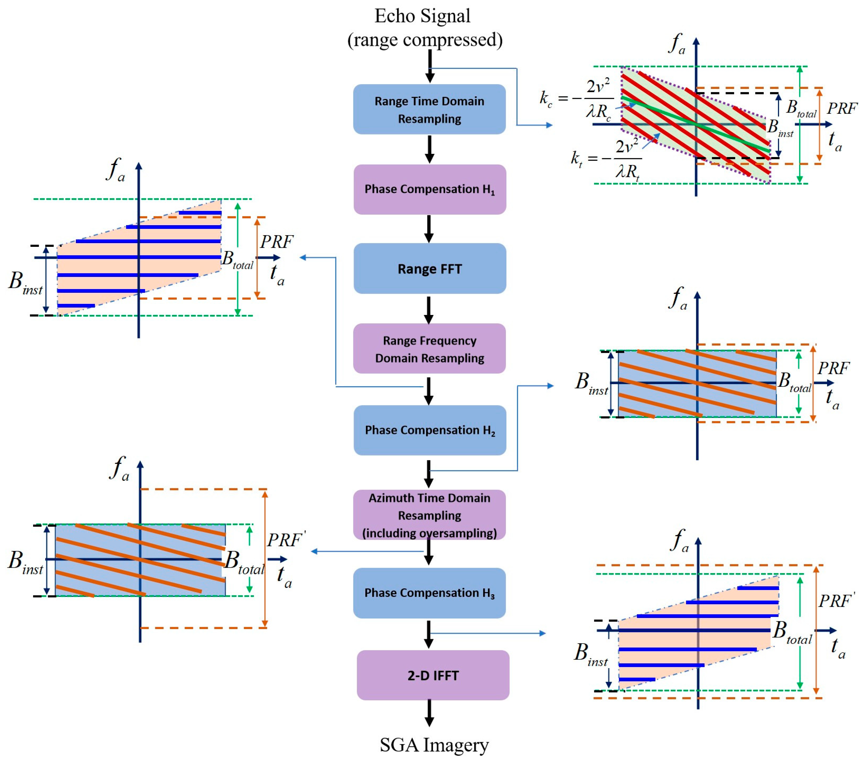
In order to apply SGA to process sliding spotlight mode data, an improved SGA is proposed. Compared to the classical SGA algorithm, the modified algorithm mainly differs in azimuth resampling and azimuth IFFT processing. The purpose of the modification is to prevent signal undersampling during azimuth resampling and azimuth IFFT processing. In order to solve the undersampling problem of the azimuth signal during azimuth resampling, the new algorithm adds a phase correction processing before the azimuth resampling to eliminate the variation of the instantaneous Doppler central frequency so that the total signal bandwidth is equal to the instantaneous bandwidth, which ensures that the PRF meets the sampling requirements. Azimuth resampling can then be performed correctly on the corrected data. However, after azimuth resampling, the azimuth signal becomes an LFM signal again due to the phase correction before azimuth resampling. Therefore, direct IFFT cannot produce a focused image. To obtain a focused image, the induced phase error should be eliminated again after azimuth resampling. Paradoxically, on the one hand, the signal has been expected to become a single-frequency signal after the phase correction, so the following IFFT can produce a focused image. But on the other hand, the instantaneous central frequency of the signal begins to change linearly again, and the total bandwidth increases, resulting in image folding after IFFT for the scene edge scatterers. To avoid image folding, the sampling rate can be appropriately increased during azimuth resampling to ensure that the signal satisfies the Nyquist sampling theorem. Based on the above solution, the processing flow of the proposed modified SGA is shown in Figure 3. The detailed analytical derivation of the algorithm is given below.

The first step of modified SGA is also range preprocessing, including range resampling, phase compensation, and range Fourier transform. The range resampling is actually to achieve a change of variable in the range time domain as follows:

$$t_r={\displaystyle \frac{2}{c}}\sqrt{R^2+R_0^2-Rc{\overline{t}}_r},$$

(3)

where ${\overline{t}}_r$ is the new time variable.

After range time domain resampling, the transformed signal can be represented as

$$\begin{array}{l}S\left(t_a,{\overline{t}}_r\right)=\mathrm{rect}\left[\left(t_a-{\displaystyle \frac{R_c{x}_t}{\left(R_c-R_s\right)v}}\right)/T_a\right]\\ \hspace{1em}\hspace{1em}\cdot \sin \mathrm{c}\left({\overline{B}}_r\left({\overline{t}}_r-{\displaystyle \frac{2u}{c}}\right)\right)\cdot \exp \left\{-j{\displaystyle \frac{4\pi f_c}{c}}r\right\}\end{array},$$

(4)

where $u=x_t\sin \theta +y_t\cos \theta$, ${\overline{B}}_r=-{\displaystyle \frac{R}{r}}{B}_r$.

The second step is phase correction, which multiplies the signal with a phase correction function:

$$H_1=\exp \left\{j{\displaystyle \frac{4\pi }{c}}\left[f_{c}r-{\overline{f}}_{c}u\right]\right\},$$

(5)

where ${\overline{f}}_c=-{\displaystyle \frac{R}{r}}{f}_c$.

After phase compensation, the signal becomes

$$\begin{array}{l}S\left(t_a,{\overline{t}}_r\right)=\mathrm{rect}\left[\left(t_a-{\displaystyle \frac{R_c{x}_t}{\left(R_c-R_s\right)v}}\right)/T_a\right]\\ \hspace{1em}\hspace{1em}\cdot \sin \mathrm{c}\left({\overline{B}}_r\left({\overline{t}}_r-{\displaystyle \frac{2u}{c}}\right)\right)\cdot \exp \left\{-j{\displaystyle \frac{4\pi {\overline{f}}_c}{c}}u\right\}\end{array}.$$

(6)

Then, performing a range FFT results in

$$\begin{array}{l}S\left(t_a,f_r\right)=\mathrm{rect}\left[\left(t_a-{\displaystyle \frac{R_c{x}_t}{\left(R_c-R_s\right)v}}\right)/T_a\right]\\ \hspace{1em}\hspace{1em}\cdot \mathrm{rect}\left({\displaystyle \frac{f_r}{{\overline{B}}_r}}\right)\cdot \exp \left\{-j{\displaystyle \frac{4\pi }{c}}\left({\overline{f}}_c+f_r\right)u\right\}\end{array}.$$

(7)

Inserting $u=x_t\sin \theta +y_t\cos \theta$ into Equation (7), we obtain

$$\begin{array}{l}S\left(t_a,f_r\right)=\mathrm{rect}\left[\left(t_a-{\displaystyle \frac{R_c{x}_t}{\left(R_c-R_s\right)v}}\right)/T_a\right]\cdot \mathrm{rect}\left({\displaystyle \frac{f_r}{{\overline{B}}_r}}\right)\\ \hspace{1em}\hspace{1em}\cdot \exp \left\{-j{\displaystyle \frac{4\pi }{c}}\left({\overline{f}}_c+f_r\right)\left(x_t\sin \theta +y_t\cos \theta \right)\right\}\end{array}.$$

(8)

Now, the signal is a 2-D discrete sample of the spectrum of the target function, but in polar format. In order to implement fast Fourier reconstruction using IFFT, it is necessary to convert polar format sampling data into rectangular format sampling data. The process of polar format conversion is actually a 2-D signal decoupling process, usually achieved through two 1-D resamplings in range and azimuth, respectively. The range resampling is essentially a scaling transformation of the range frequency as follows:

$$f_r={\delta }_r{\overline{f}}_r+{\overline{f}}_{\mathrm{c}}\left({\delta }_r-1\right),$$

(9)

where ${\delta }_r=1/cos\theta$.

After range resampling, the signal becomes

$$\begin{array}{l}S\left(t_a,{\overline{f}}_r\right)=\mathrm{rect}\left[\left(t_a-{\displaystyle \frac{R_c{x}_t}{\left(R_c-R_s\right)v}}\right)/T_a\right] \cdot \mathrm{rect}\left({\displaystyle \frac{{\overline{f}}_r}{{\overline{B}}_r}}\right)\\ \hspace{1em}\hspace{1em}\hspace{1em}\hspace{1em}\cdot \exp \left\{-j{\displaystyle \frac{4\pi }{c}}\left({\overline{f}}_c+{\overline{f}}_r\right)\left(x_t\tan \theta +y_t\right)\right\}\end{array}.$$

(10)

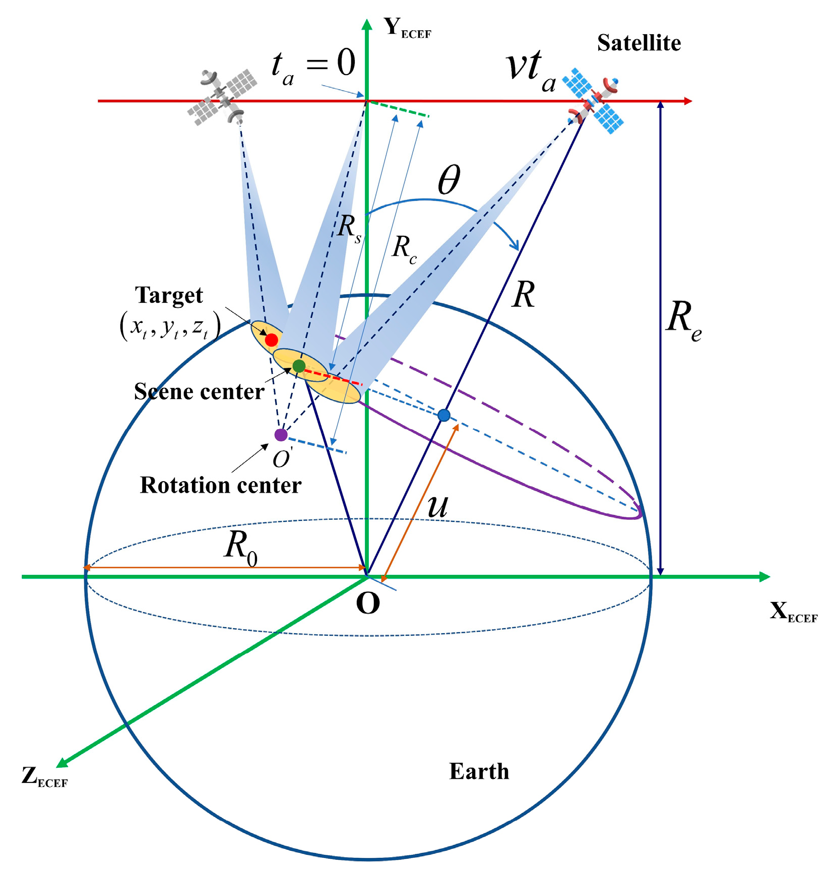
From the data collection geometry shown in Figure 1, it is easy to calculate that $\tan \theta =v{t}_a/R_e$. Therefore, Equation (10) can also be rewritten as

$$\begin{array}{l}S\left(t_a,{\overline{f}}_r\right)=\mathrm{rect}\left[\left(t_a-{\displaystyle \frac{R_c{x}_t}{\left(R_c-R_s\right)v}}\right)/T_a\right]\cdot \mathrm{rect}\left({\displaystyle \frac{{\overline{f}}_r}{{\overline{B}}_r}}\right)\\ \hspace{1em}\hspace{1em}\cdot \exp \left\{-j{\displaystyle \frac{4\pi }{c}}\left({\overline{f}}_c+{\overline{f}}_r\right)\left(x_t{\displaystyle \frac{v}{R_e}}{t}_a+y_t\right)\right\}\end{array}.$$

(11)

In standard SGA processing for spotlight mode data, the next step is an azimuth resampling. However, for the sliding spotlight mode, due to the residual variation of the instantaneous Doppler central frequency, the signal at this point often does not satisfy the Nyquist sampling theorem. In order to ensure that azimuthal resampling yields correct results, it is necessary to compensate for the variation of instantaneous Doppler central frequency, which can be implemented by multiplying the signal with the following phase correction function.

$$H_2=\exp \left\{-j\pi \left(k_c-k_t\right)t_a^2\right\}.$$

(12)

After this correction, the signal becomes

$$\begin{array}{l}S\left(t_a,{\overline{f}}_r\right)=\mathrm{rect}\left[\left(t_a-{\displaystyle \frac{R_c{x}_t}{\left(R_c-R_s\right)v}}\right)/T_a\right]\cdot \mathrm{rect}\left({\displaystyle \frac{{\overline{f}}_r}{{\overline{B}}_r}}\right)\\ \hspace{1em}\hspace{1em}\cdot \exp \left\{-j\left[{\displaystyle \frac{4\pi }{c}}\left({\overline{f}}_c+{\overline{f}}_r\right)\left(x_t{\displaystyle \frac{v}{R_e}}{t}_a+y_t\right)+\pi \left(k_c-k_t\right)t_a^2\right]\right\}\end{array}.$$

(13)

Now, the signal satisfies the Nyquist sampling theorem and can be resampled in the azimuth direction. The azimuth resampling is mathematically a keystone transform as follows:

$$t_a={\displaystyle \frac{{\overline{f}}_c}{{\overline{f}}_c+{\overline{f}}_r}}{\overline{t}}_a.$$

(14)

Therefore, after azimuth resampling, the signal becomes

$$\begin{array}{l}S\left({\overline{t}}_a,{\overline{f}}_r\right)=\mathrm{rect}\left[\left({\overline{t}}_a-{\displaystyle \frac{R_c{x}_t}{\left(R_c-R_s\right)v}}\right)/T_a\right]\cdot \mathrm{rect}\left({\displaystyle \frac{{\overline{f}}_r}{{\overline{B}}_r}}\right)\\ \hspace{1em}\cdot \exp \left\{-j\left[{\displaystyle \frac{4\pi v}{\overline{\lambda }{R}_e}}{\overline{t}}_a\cdot x_t+{\displaystyle \frac{4\pi }{c}}\left({\overline{f}}_c+{\overline{f}}_r\right)\cdot y_t+\pi \left(k_c-k_t\right){\left({\displaystyle \frac{{\overline{f}}_c}{{\overline{f}}_c+{\overline{f}}_r}}{\overline{t}}_a\right)}^2\right]\right\}\end{array},$$

(15)

where $\overline{\lambda }=c/{\overline{f}}_c$.

The multiplication of phase function $H_2$ before azimuth resampling ensures the correct implementation of azimuth resampling on one hand, but also introduces an additional phase error on the other hand. To eliminate its adverse effect, it is necessary to multiply the resampled signal by the following correction function:

$$H_3=\exp \left\{j\left[\pi \left(k_c-k_t\right){\left({\displaystyle \frac{{\overline{f}}_c}{{\overline{f}}_c+{\overline{f}}_r}}{\overline{t}}_a\right)}^2\right]\right\}.$$

(16)

After this correction, the signal becomes

$$\begin{array}{l}S\left({\overline{t}}_a,{\overline{f}}_r\right)=\mathrm{rect}\left[\left({\overline{t}}_a-{\displaystyle \frac{R_c{x}_t}{\left(R_c-R_s\right)v}}\right)/T_a\right]\cdot \mathrm{rect}\left({\displaystyle \frac{{\overline{f}}_r}{{\overline{B}}_r}}\right)\\ \hspace{1em}\hspace{1em}\cdot \exp \left\{-j\left[{\displaystyle \frac{4\pi v}{\overline{\lambda }{R}_e}}{\overline{t}}_a\cdot x_t+{\displaystyle \frac{4\pi }{c}}\left({\overline{f}}_c+{\overline{f}}_r\right)\cdot y_t\right]\right\}\end{array}.$$

(17)

At this point, the signal is completely 2-D decoupled and becomes a sinusoidal signal in both dimensions, with frequency linearly related to the target’s position. Therefore, a final 2-D IFFT can produce focused imagery. However, from the time–frequency diagram at this point in Figure 3, it is clear that the total azimuth bandwidth is still greater than the instantaneous bandwidth. To avoid image folding, the sampling rate can be appropriately increased during azimuth resampling. The oversampling factor is determined by the ratio of the total bandwidth to the instantaneous bandwidth. Since each target at different azimuth positions corresponds to a distinct azimuth frequency, the total azimuth bandwidth depends on the entire scene width, while the instantaneous bandwidth is determined by the scene width illuminated by the instantaneous azimuth beamwidth. Consequently, the ratio of the total signal bandwidth to the instantaneous bandwidth equals the ratio of the total scene width to the instantaneous beam coverage width. For example, if the scene width covered by the instantaneous azimuth beamwidth is $W_{beam}$, and the total scene width scanned by the beam during the coherent integration time is $W_{total}$, the oversampling factor for the azimuth interpolation is $W_{total}/W_{beam}$.

Now, a 2-D IFFT can produce unfolded imagery. Firstly, by performing an azimuth IFFT on Equation (17), we obtain

$$\begin{array}{l}S\left({\overline{f}}_a,{\overline{f}}_r\right)=\sin \mathrm{c}\left[T_a\left({\overline{f}}_a-{\displaystyle \frac{2v}{\overline{\lambda }{R}_e}}{x}_t\right)\right]\cdot \mathrm{rect}\left({\displaystyle \frac{{\overline{f}}_r}{{\overline{B}}_r}}\right)\\ \hspace{1em}\hspace{1em}\hspace{1em}\hspace{1em}\cdot \exp \left\{-j\left[{\displaystyle \frac{4\pi }{c}}\left({\overline{f}}_c+{\overline{f}}_r\right)\cdot y_t\right]\right\}\end{array}.$$

(18)

Then, performing a range IFFT results in the following 2-D focused imagery:

$$S\left({\overline{f}}_a,{\overline{t}}_r\right)=A\cdot \sin \mathrm{c}\left[T_a\left({\overline{f}}_a-{\displaystyle \frac{2v}{\overline{\lambda }{R}_e}}{x}_t\right)\right]\cdot \sin \mathrm{c}\left[{\overline{B}}_r\left({\overline{t}}_r-{\displaystyle \frac{2}{c}}{y}_t\right)\right].$$

(19)

If we define $x={\displaystyle \frac{\overline{\lambda }{R}_e}{2v}}{\overline{f}}_a$, $y={\displaystyle \frac{c}{2}}{\overline{t}}_r$, Equation (19) can also be expressed as

$$S\left(x,y\right)=A\cdot \sin \mathrm{c}\left[{\displaystyle \frac{2v{T}_a}{\overline{\lambda }{R}_e}}\left(x-x_t\right)\right]\cdot \sin \mathrm{c}\left[{\displaystyle \frac{2{\overline{B}}_r}{c}}\left(y-y_t\right)\right]$$

(20)

Now, the target is accurately focused at its true position in the orbit plane.

Next, we evaluate the computational performance of the modified algorithm. Both the standard SGA and modified SGA processing flows involve only three types of operations: complex multiplication, interpolation, and FFT/IFFT. Specifically, the original SGA requires one complex multiplication, three interpolation operations, and three 1-D FFT/IFFT operations, while the improved algorithm requires three complex multiplications, three interpolation operations, and three 1D FFT/IFFT operations. Consequently, the improved algorithm introduces two additional complex multiplications compared to the original algorithm. Furthermore, azimuth resampling necessitates a slightly higher sampling rate, leading to increased computational load in the azimuth interpolation process and subsequent phase compensation and azimuth IFFT steps due to the expanded data volume.

4. Experimental Results and Discussion

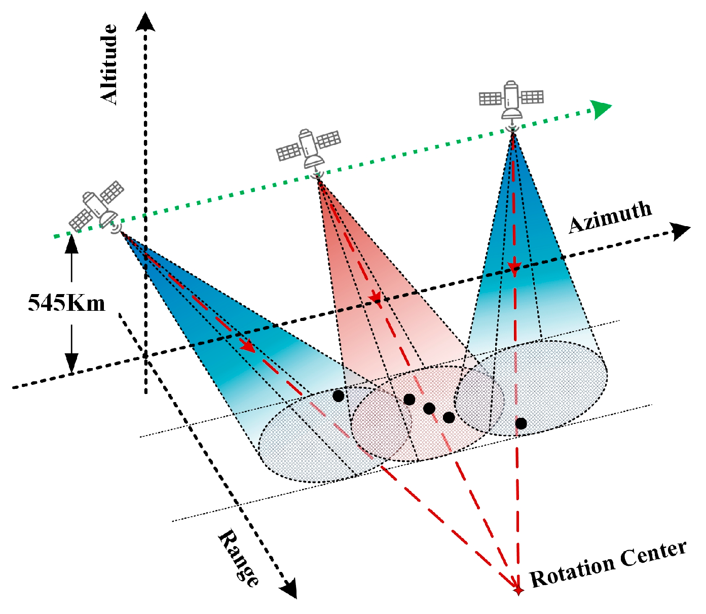
To validate the performance of the algorithm, both simulation and real data processing are carried out. In the simulation experiment, the imaging geometry is shown in Figure 4. The radar is operated in sliding spotlight mode, where the scene center range is 600 km and the rotation center range is 900 km. Some main radar parameters are listed in

Table 1. Main radar parameters for simulation.

Parameter	Value	Parameter	Value
Carrier frequency (GHz)	9.6	PRF (Hz)	4000
Pulse width (μs)	10	Beam width (°)	0.3
Bandwidth (MHz)	500	Scene center range (km)	600
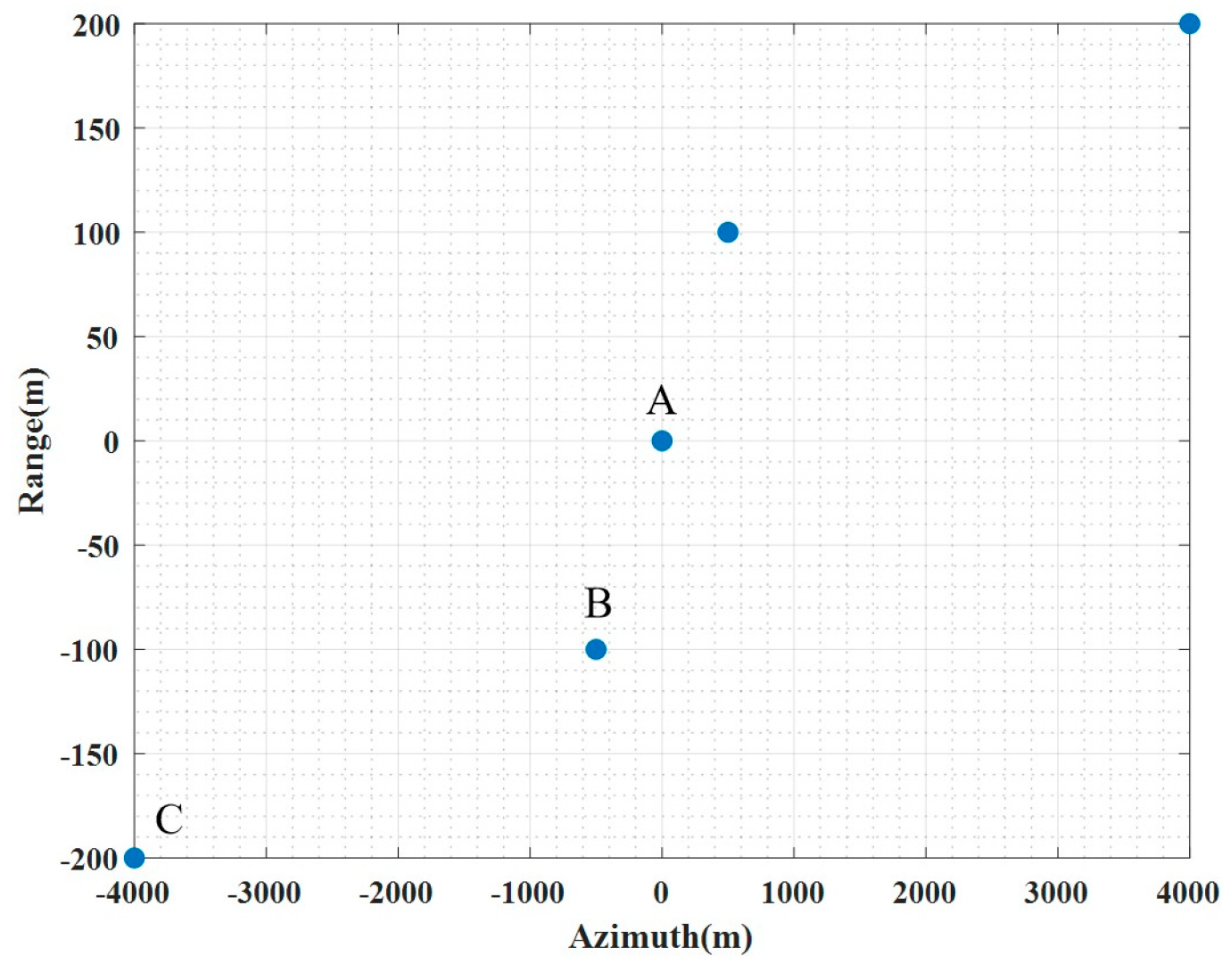
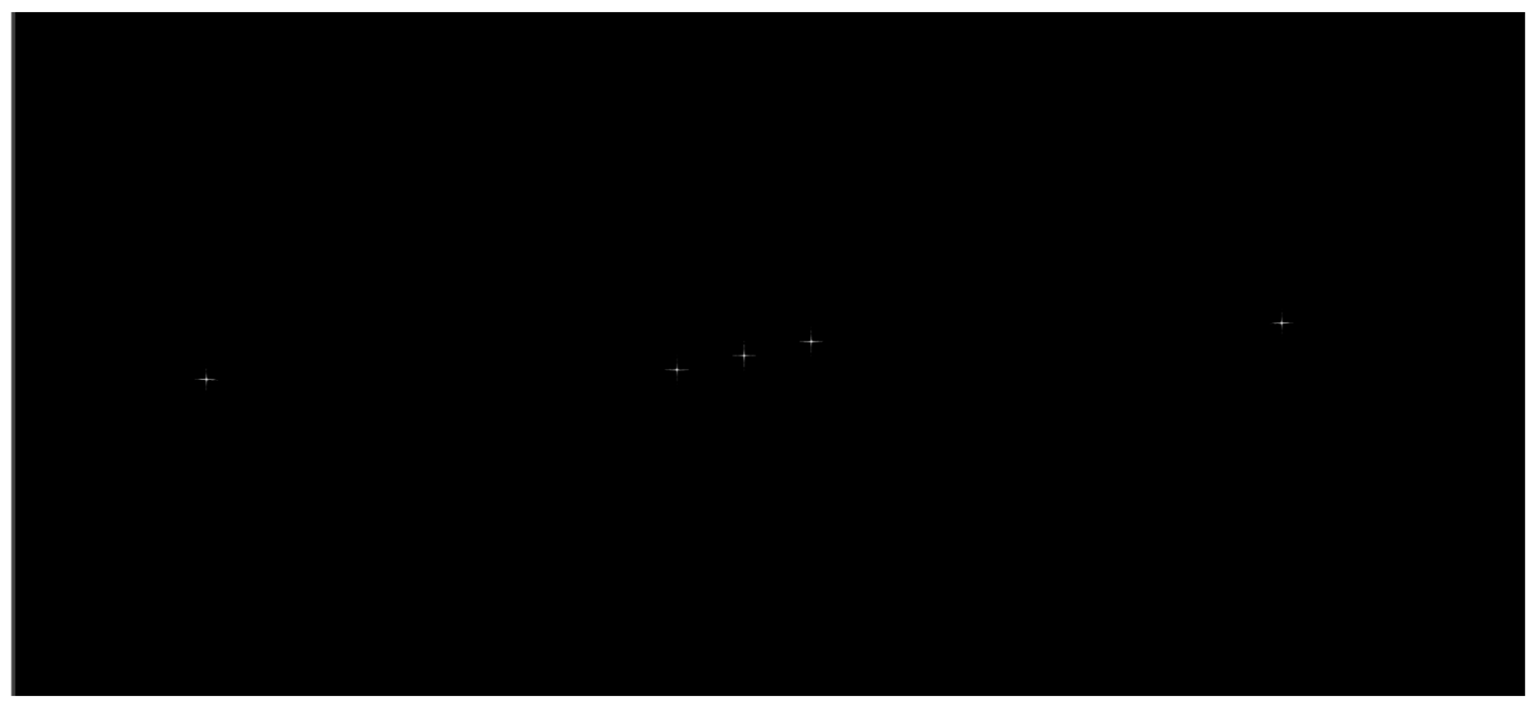
Sample rate (MHz)	600	Rotation center range (km)	900

. Five point targets with different positions were placed within the imaging scene as shown in Figure 5.

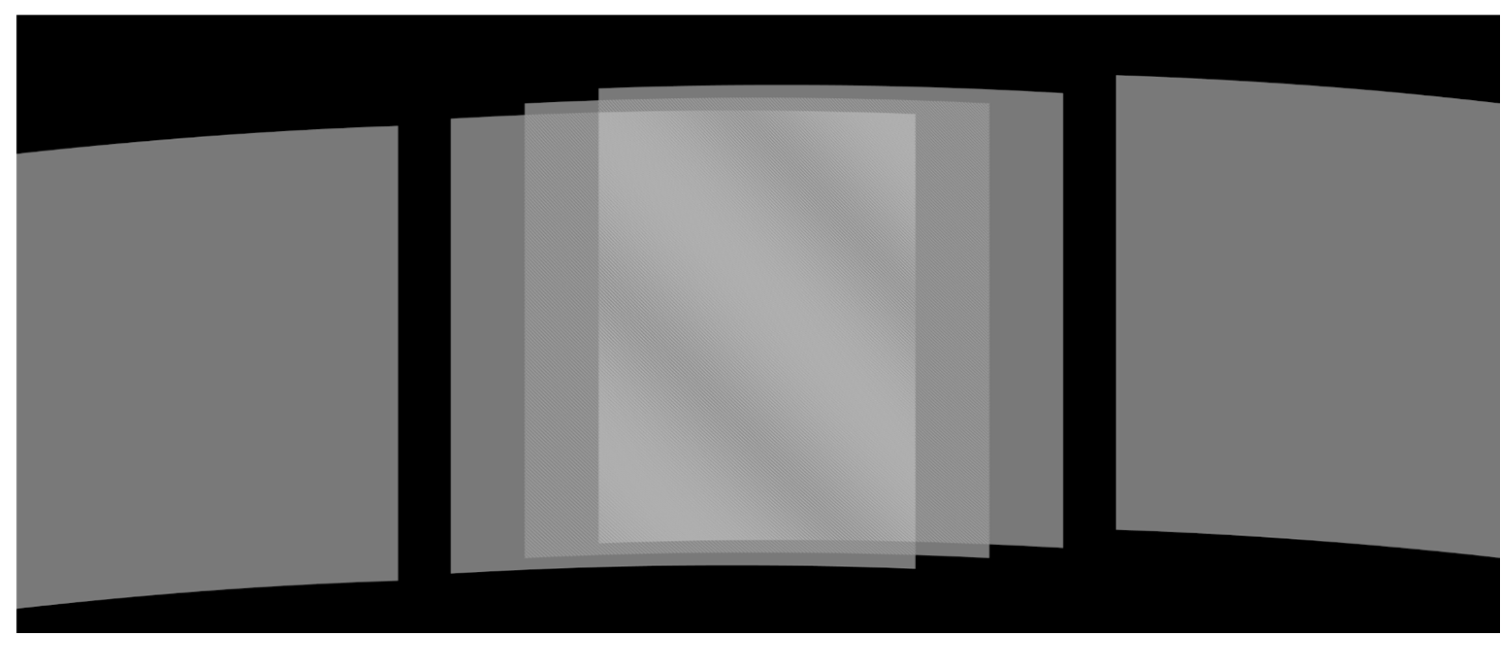
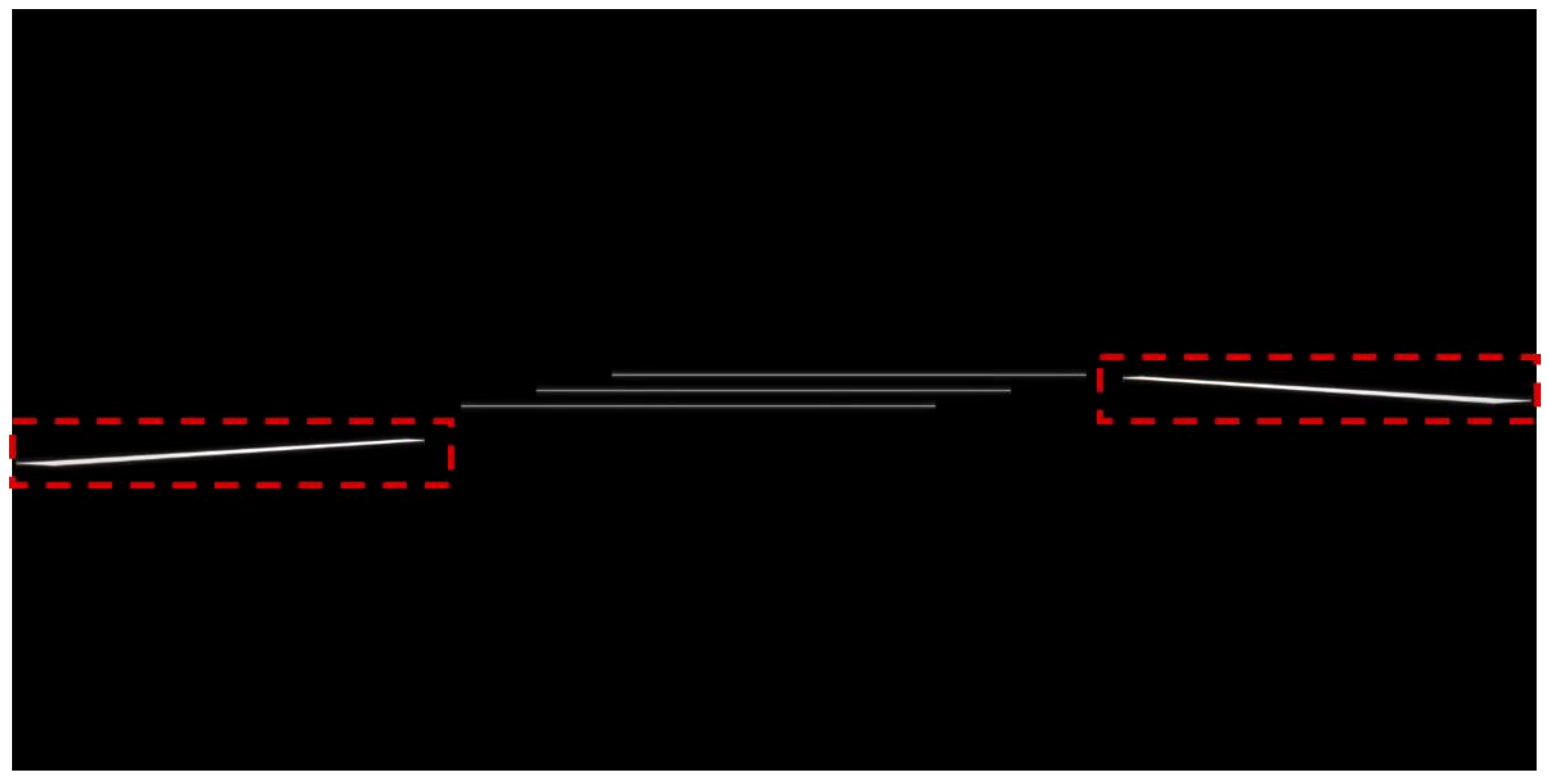
The simulated raw data are shown in Figure 6. The data are first processed by the standard SGA, and the produced image is shown in Figure 7 and Figure 8, where Figure 7 is the range-compressed imagery and Figure 8 is the full-compressed imagery. As can be seen from the figures, only the targets near the center of the scene are accurately focused, while the targets at the edges of the azimuth suffer from being severely 2-D defocused on the one hand, and the positions of the targets, on the other hand, are also aliased. This is because the signals of targets located at the edge of the azimuth scene are undersampled during both azimuth interpolation and azimuth IFFT processing. The undersampling during azimuth interpolation prevents complete correction of the range migration, resulting in 2-D defocusing in the final image, while the undersampling during azimuth IFFT causes aliasing of the target’s azimuth position.

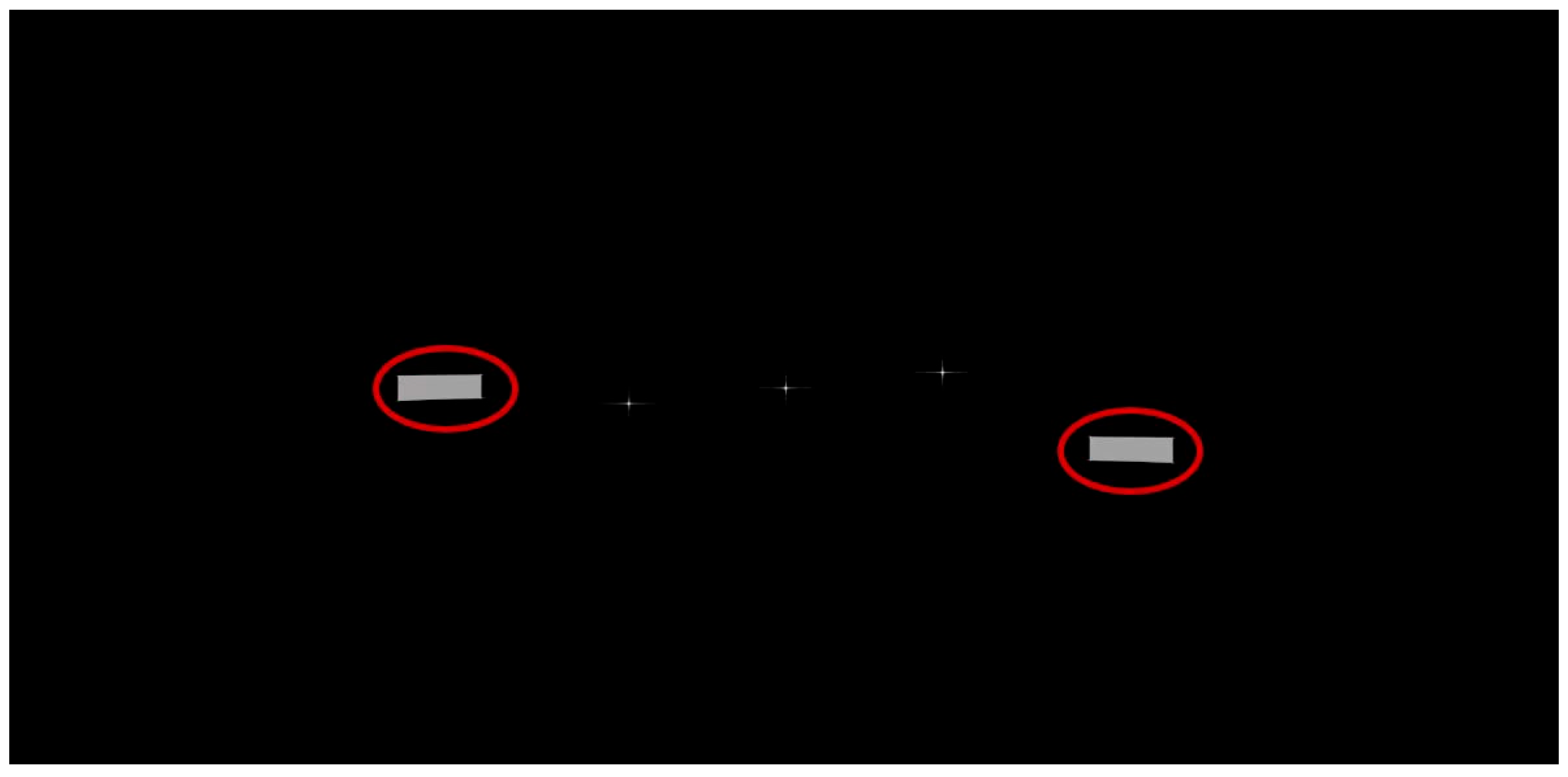
Finally, the data are also processed using the modified SGA algorithm, and the processing results are shown in Figure 9 and Figure 10, where Figure 9 is the range-compressed image and Figure 10 is the full-compressed image. From Figure 9, it is clear that the range migration of scatterers located at the scene edge is also completely eliminated. Then, these point targets are also well focused, as shown in Figure 10.

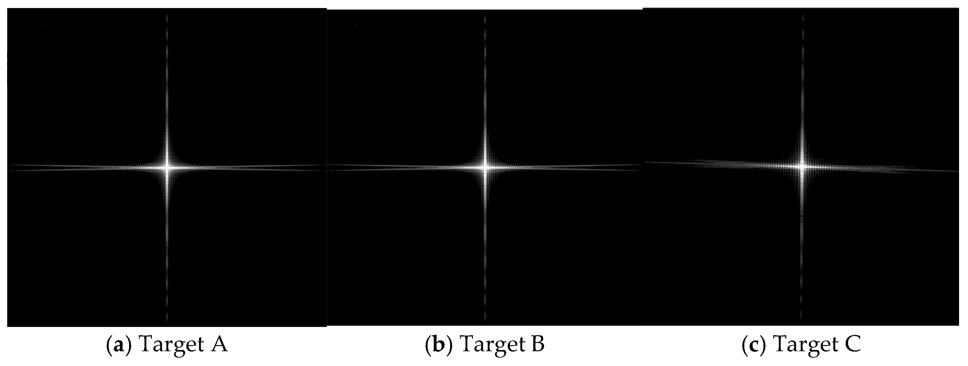
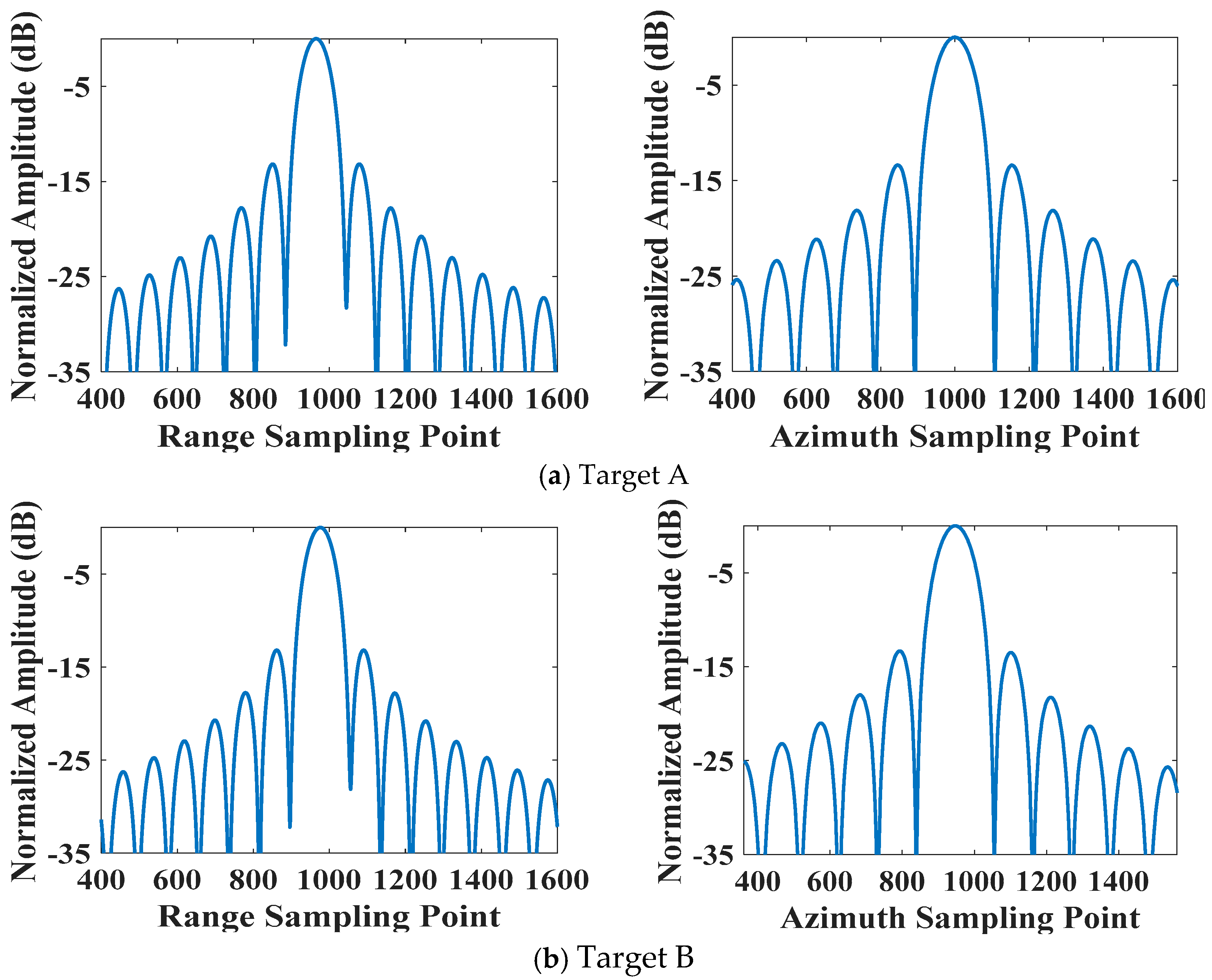
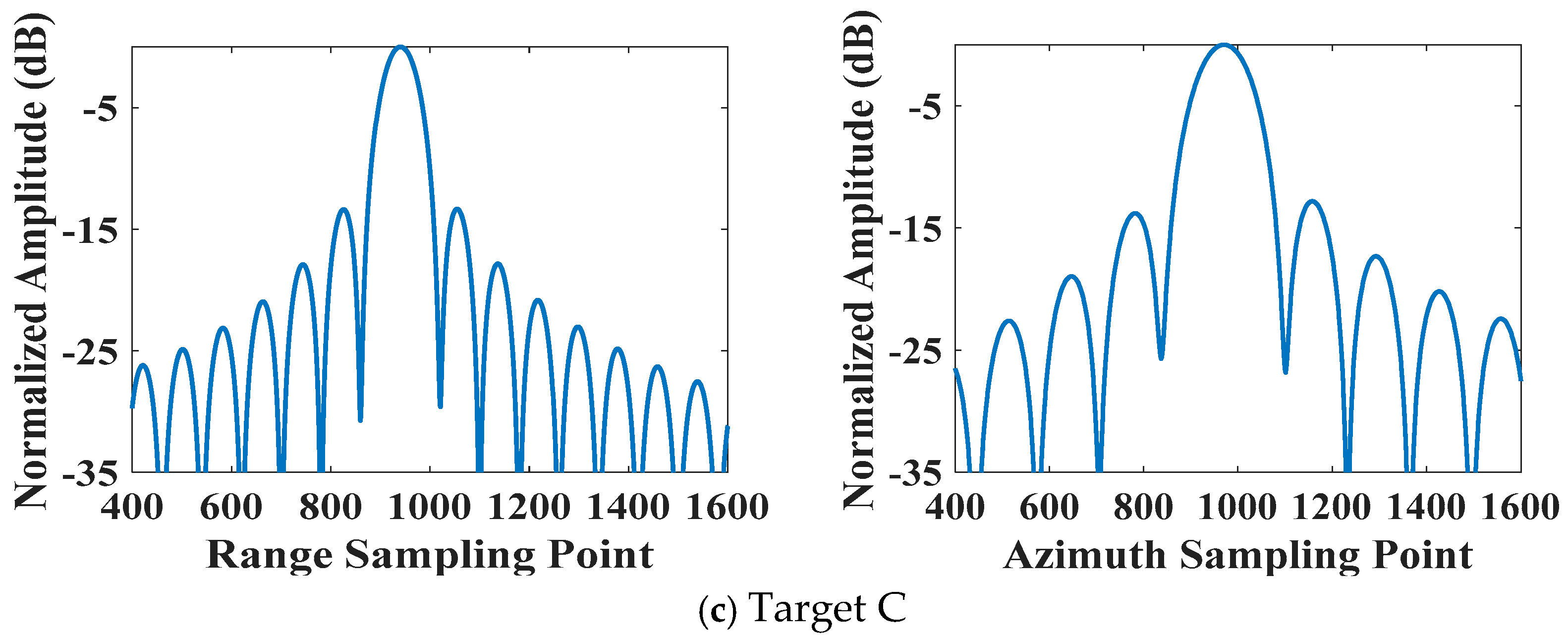
To evaluate the focus accuracy, point target analysis is performed for the three targets A, B, and C in the modified SGA image. First, the 2-D impulse response functions (IRFs) are shown in Figure 11. Also, the range and azimuth profiles are given in Figure 12. To quantitatively evaluate the focusing performance, the image quality parameters of these IRFs, including the impulse response width (IRW), peak sidelobe ratio (PSLR), and integrated sidelobe ratio (ISLR), are listed in

Table 2. Image quality parameters.

		Target A	Target B	Target C
Range	IRW (m)	0.7567	0.7567	0.7567
	PSLR (dB)	−13.1824	−13.1843	−13.3422
	ISLR(dB)	−9.9428	−9.9498	−10.1313
Azimuth	IRW (m)	0.9880	0.9972	1.2188
	PSLR (dB)	−13.3978	−13.3429	−13.0156
	ISLR(dB)	−10.3072	−10.2993	−10.3565

. These metrics demonstrate that all targets have been accurately focused. The resolution of Target C is slightly inferior to other targets, which is attributed to its relatively shorter illumination time.

The proposed algorithm is also validated using measured spaceborne SAR data. The data were collected by a LEO SAR satellite with an orbit height of 540 km. During this data collection, the radar operated in sliding spotlight mode. Some main orbit and radar parameters are shown in

Table 3. Main radar parameters of real data.

Parameter	Value	Parameter	Value
Carrier frequency (GHz)	9.6	Coherent time (s)	3
Pulse width (μs)	25	Orbit altitude (km)	540
Bandwidth (MHz)	500	Scene size (km × km)	6 × 15
Sample rate (MHz)	600	Scene center range (km)	610
PRF (Hz)	4200	Rotation center range (km)	720

.

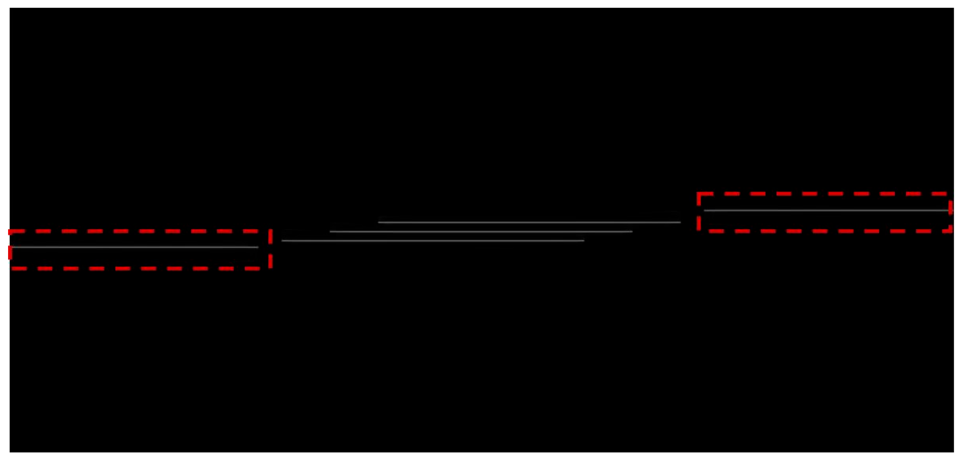
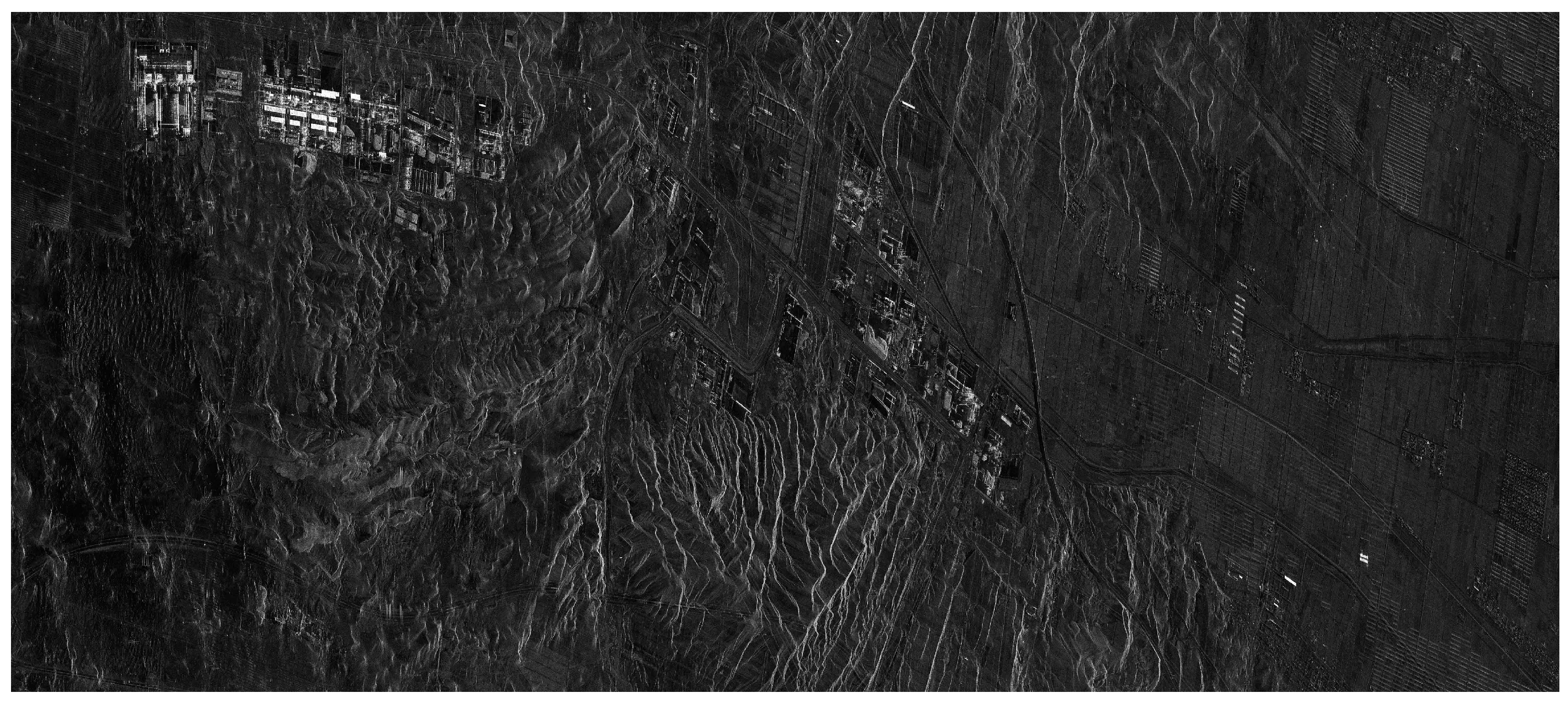
Firstly, the data are processed by the classical SGA, and the result is presented in Figure 13. As can be seen from the figure, the scatterers near the scene center are all well-focused and accurately located at their true positions. But for the scatterers at the azimuth edge of the scene, they are aliased in the produced image, and on the other hand, these scatterers also suffer from defocus due to residual linear range migration, which has not been corrected during azimuth resampling.

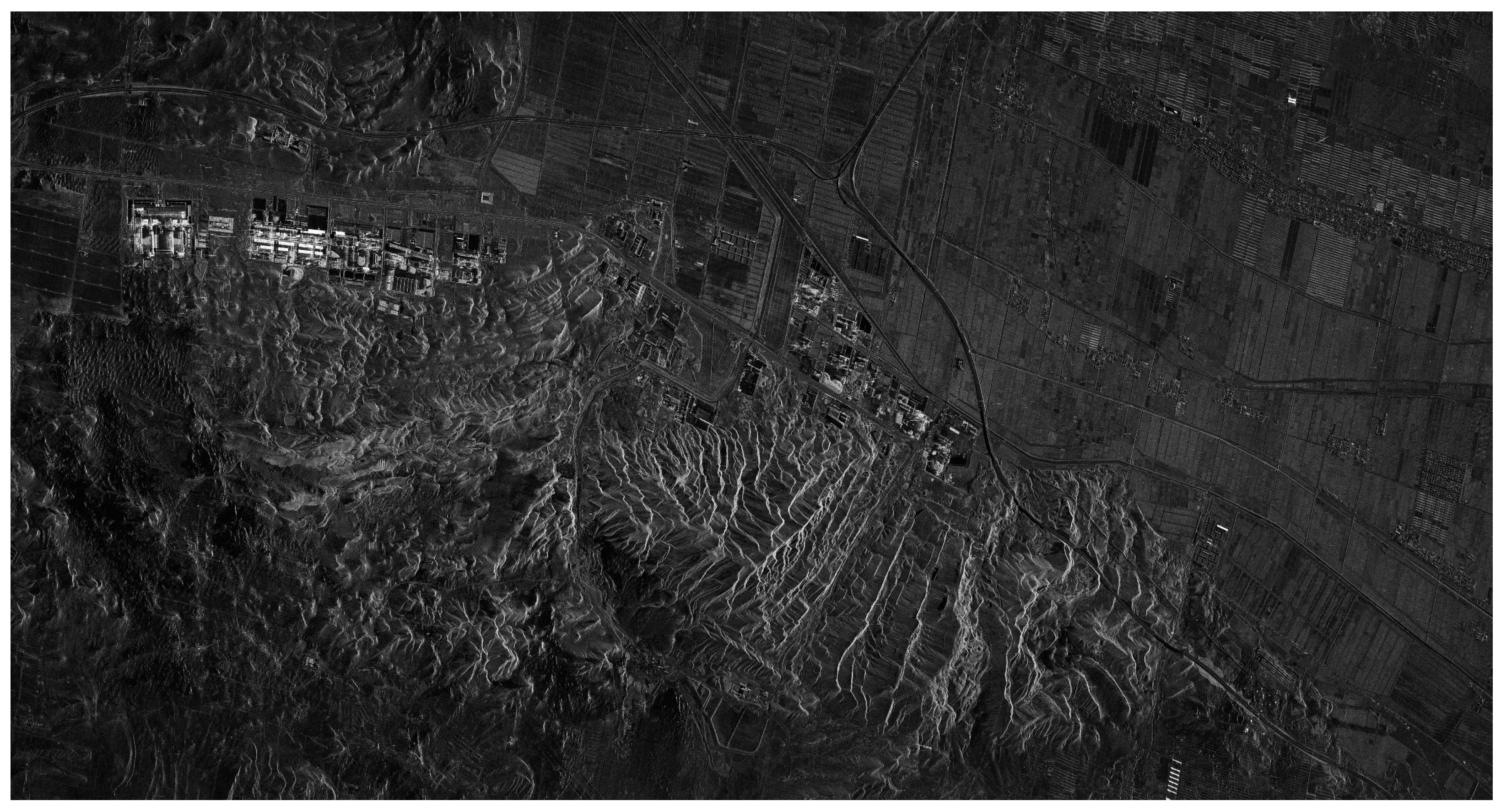
Then, the data are also processed by the proposed algorithm, and the result is shown in Figure 14. It can be seen that all scatterers in the scene have been accurately focused and located at their true positions.

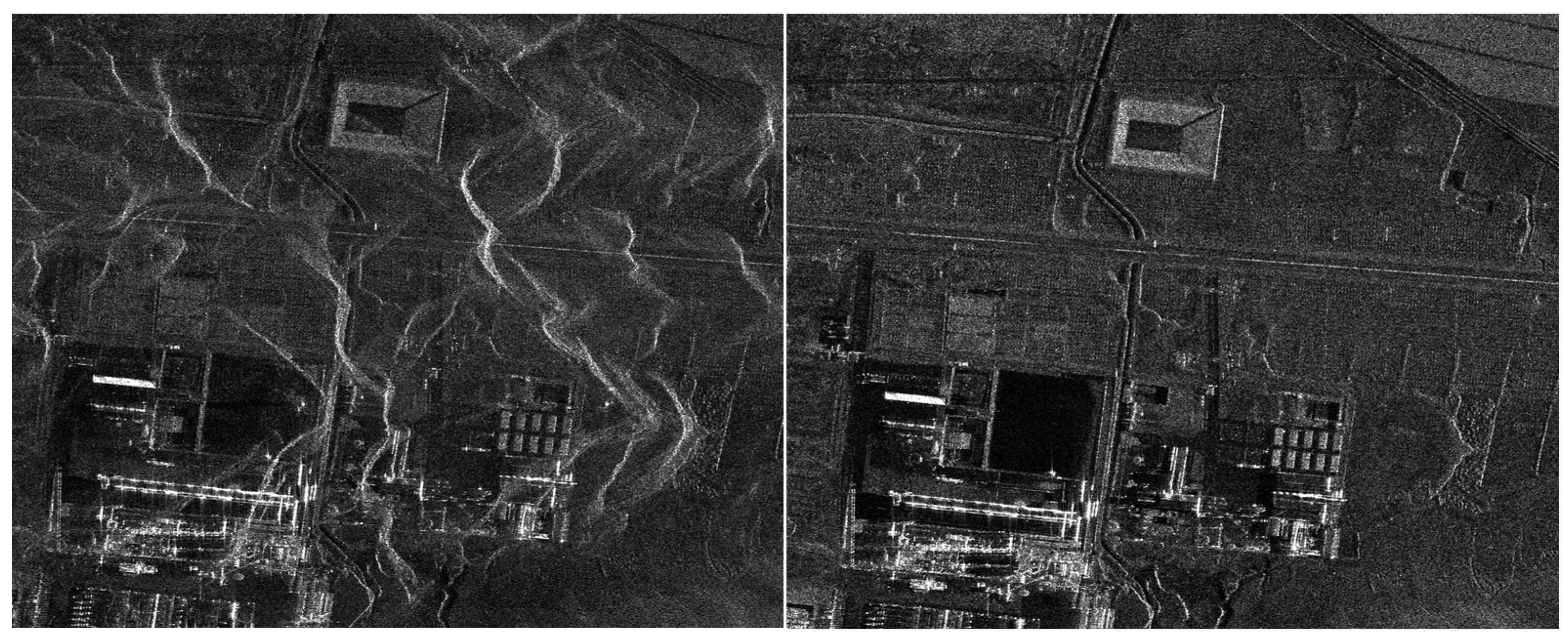
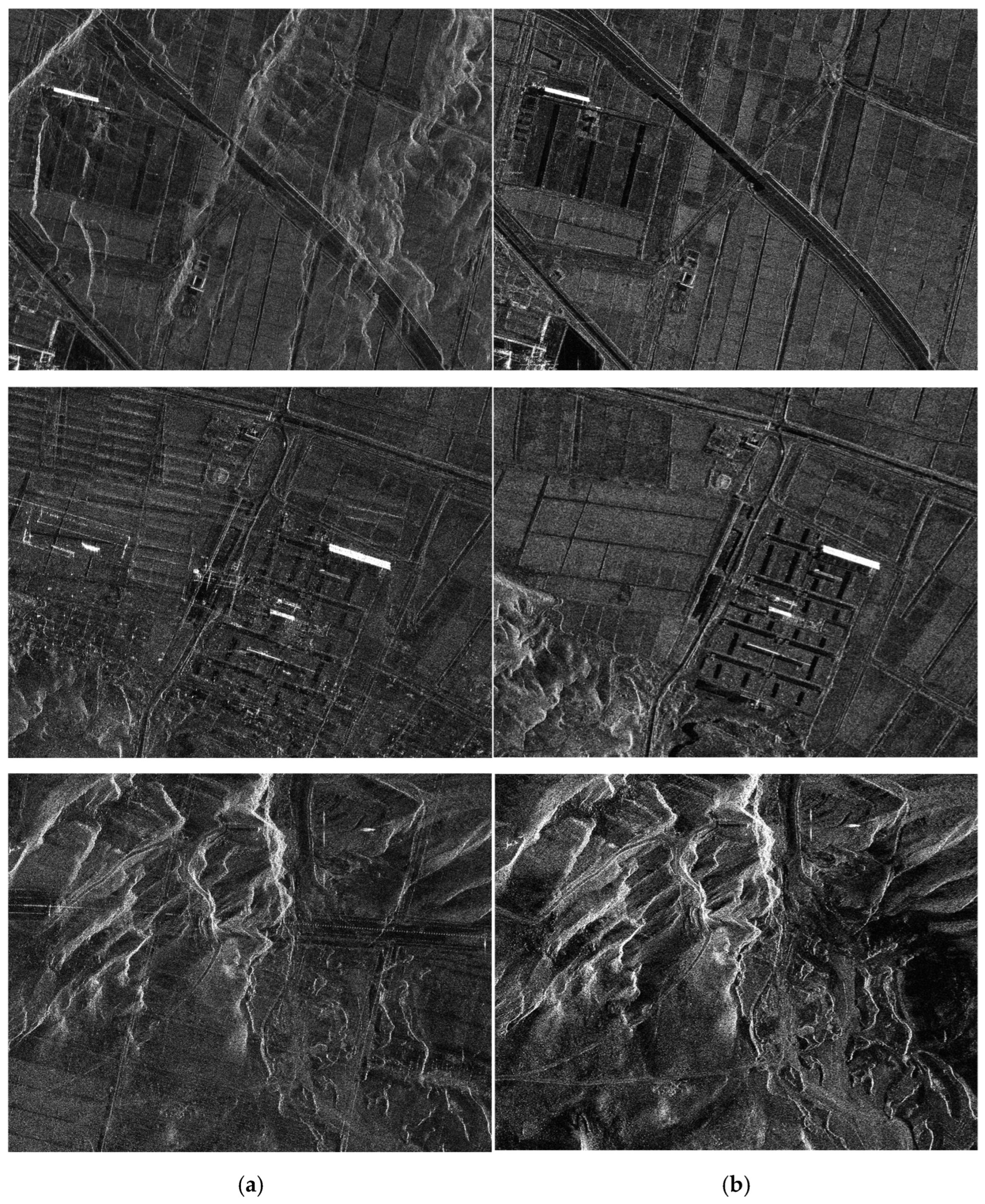
To see the performance improvement more clearly, some local subimages in the same area in both figures are presented in Figure 15, where Figure 15a shows the subimages from Figure 13, and Figure 15b shows the corresponding subimages in Figure 14. Comparison results show clearly that the aliasing effect presented in the standard SGA image is completely eliminated in the modified SGA image.

In order to quantitatively assess the focusing performance of both algorithms, the measured image contrast and image entropy of Figure 13 and Figure 14 are shown in

Table 4. Comparison of image quality index.

	SGA	Modified SGA
Contrast	27.056	29.817
Entropy	21.582	18.952

. The results show that the imagery produced by the proposed approach has a higher contrast value and smaller entropy value. Therefore, the comparison results also show that the imagery produced by the modified SGA has better focus quality.

5. Conclusions

Standard SGA was proposed for processing spotlight mode SAR data and cannot be directly applied to process sliding spotlight SAR data. In this paper, an extended SGA for processing sliding spotlight mode SAR data is proposed. The modified algorithm extends the application of the original algorithm. Experimental results verify the validity of the proposed approach. Next, we will further extend the algorithm to other modes, such as stripmap, TOPS, etc. The main challenge in extending to other modes is how to address the aliasing issue in azimuth compression when scenarios expand. Although the proposed algorithm can solve this by increasing the azimuth sampling rate, data volume would surge dramatically when extended to stripmap or TOPS modes. How to avoid image aliasing without significantly increasing data volume remains a key research question for our next steps.