Enhancing DeepLabv3+ Convolutional Neural Network Model for Precise Apple Orchard Identification Using GF-6 Remote Sensing Images and PIE-Engine Cloud Platform

Abstract

Utilizing remote sensing models to monitor apple orchards facilitates the industrialization of agriculture and the sustainable development of rural land resources. This study enhanced the DeepLabv3+ model to achieve superior performance in apple orchard identification by incorporating ResNet, optimizing the algorithm, and adjusting hyperparameter configuration using the PIE-Engine cloud platform. GF-6 PMS images were used as the data source, and Qixia City was selected as the case study area for demonstration. The results indicate that the accuracies of apple orchard identification using the proposed DeepLabv3+_34, DeepLabv3+_50, and DeepLabv3+_101 reached 91.17%, 92.55%, and 94.37%, respectively. DeepLabv3+_101 demonstrated superior identification performance for apple orchards compared with ResU-Net and LinkNet, with an average accuracy improvement of over 3%. The identified area of apple orchards using the DeepLabv3+_101 model was 629.32 km², accounting for 31.20% of Qixia City’s total area; apple orchards were mainly located in the western part of the study area. The innovation of this research lies in combining image annotation and object-oriented methods during training, improving annotation efficiency and accuracy. Additionally, an enhanced DeepLabv3+ model was constructed based on GF-6 satellite images and the PIE-Engine cloud platform, exhibiting superior performance in feature expression compared with conventional machine learning classification and recognition algorithms.

1. Introduction

Apple cultivation holds a significant position with extensive influence within China’s agricultural industry [1,2]. According to statistics, China’s annual apple production reached 37,349,700 tons in 2024, ranking it first globally. To provide the government with essential data support for formulating agricultural policies and effective management, it is necessary to promptly understand the spatial distribution patterns and scale of apple orchards. However, conventional field survey methods for orchards are labor-intensive and subjective, posing challenges in obtaining accurate and comprehensive data on apple orchards [3,4]. Remote sensing technology enables rapid acquisition of real-time information over large areas and finds extensive applications in the agricultural sector [5].

Multispectral remote sensing images have been widely utilized for crop monitoring and analysis by scholars due to their extensive coverage, minimal band redundancy, strong continuity, and cost-effectiveness [6]. With the rapid advancement of remote sensing technology, there is an increasing abundance of multispectral remote sensing image types. Among them, China’s GF-6 image stands out as one of the few data sources with meter-level resolution currently available. It boasts high spectral resolution (4-band), spatial resolution (2 m), and temporal resolution (4 days) advantages over others [7], making it a potential fundamental data source for apple orchard extraction. The identification of apple orchards using high-precision identification models based on GF-6 imagery as the data source is an area that requires further investigation, given the limited number of studies conducted in this field.

As the resolution of remote sensing images gradually increases, the correlation between low-level features and high-level semantics of ground objects becomes increasingly intricate, posing challenges for traditional remote sensing identification methods to adapt. With the advantages of multidimensional feature learning, robust generalization capability, and high classification accuracy, the convolutional neural network (CNN) model has progressively emerged as one of the most accurate models for ground object remote sensing identification [8]. In the domain of regional-scale crop remote sensing identification, CNN-based remote sensing identification is predominantly employed in wheat, corn, rice, and other bulk crops research [9]. The spatial distribution of these crops is extensive, exhibiting distinct texture features that facilitate convenient labeling and identification [10]. In terms of orchard planting areas, CNNs are predominantly employed for remote sensing identification in vineyards, citrus orchards, and other similar areas characterized by well-defined boundaries, distinct textures, and meticulous planning [11,12]. Sun et al. [13] employed the DeepLabv3 model and incorporated a band enhancement (BIE) module to conduct remote sensing identification of grape planting areas based on multispectral images. Compared with other crop and orchard cultivation systems, apple orchards demonstrate characteristically dispersed spatial distribution patterns, which present unique challenges for accurate labeling and identification in remote sensing applications. Current methodologies primarily employ conventional machine learning classifiers, including K-nearest neighbor (KNN), support vector machine (SVM), and random forest (RF) algorithms, for this classification task [14].

By training on a large volume of sample data, CNN semantic segmentation models can automatically learn to extract internal laws and deep features such as crop boundaries and textures in high-resolution images [15]. This enables them to capture complex nonlinear relationships, construct deep neural networks, and enhance the accuracy of crop identification [16,17,18]. The strong spatial feature extraction capability of the proposed method facilitates fast segmentation and accurate classification of remote sensing images [19]. In 2015, U-Net introduced an encoder–decoder structure to effectively integrate high- and low-level semantic information, thereby enhancing the refinement of object spatial structures during upsampling [20]. Chaurasia and Culurciello [21] proposed LinkNet in 2017 as a lightweight fully convolutional neural network that also adopts an encoder-decoder architecture to enhance information transfer efficiency and reduce training time. In order to achieve enhanced training effectiveness, the mainstream network structure has been progressively deepened. However, this has led to increased difficulty in model training and significant elevation of both training error and test error. To address these issues, He et al. [22] proposed ResNet, a residual network that introduced the concept of Residual Block. This innovation effectively resolves the problems of gradient disappearance and explosion as the network hierarchy deepens. Moreover, DeepLab series networks incorporate multiscale void convolution and Atrous Spatial Pyramid Pooling (ASPP) structures to further enhance semantic segmentation accuracy [23]. However, there is currently no relevant research on enhancing convolutional neural networks for remote sensing-based apple orchard extraction.

To address current challenges and limitations in remote sensing identification of apple orchards, this study employs GF-6 high-resolution satellite imagery as the primary data source to explore an accurate identification model. By integrating a convolutional neural network (CNN) for semantic segmentation with an object-oriented classification algorithm—while further optimizing the CNN architecture—we achieve precise remote sensing identification of apple orchards. This study aims to effectively enhance accuracy and efficiency in remote sensing identification of apple orchards while providing rapid and accurate modeling methods along with data support for agricultural industrialization management.

2. Study Area and Data Source

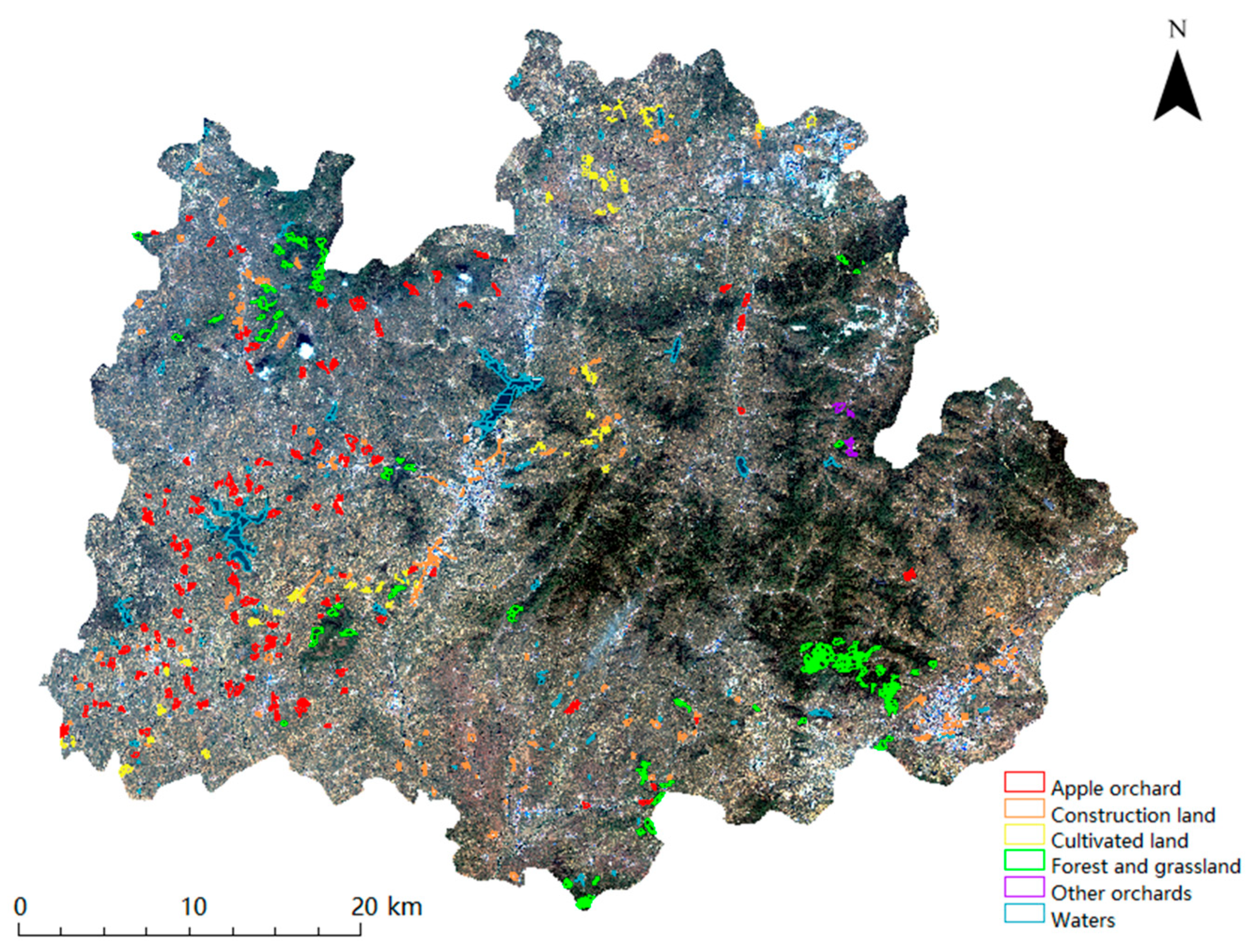
2.1. Case Study Area

Qixia City is situated between 37°05′05”–37°29′46”N and 120°32′45”–121°15′58”E, encompassing a total area of 2016.66 km². Figure 1 displays the geographical location and elevation profile of the study area, with a red star indicating the specific research site. The study area comprises 15 townships, namely Guandao, Guanli, Yangchu, Sikou, Xicheng, Shewopo, Sujiadian, Songshan, Zhuangyuan, Cuiping, Tangjiapo, Zangjiazhuang, Tingkou, Miaohou, and Taocun. The climate in this region exhibits four distinct seasons with ample sunlight and an average annual temperature of 11.3 °C, along with 650 mm rainfall and a total annual sunshine duration of 2690 h. It falls under the category of warm temperate monsoon type semi-humid climate, which is highly conducive for apple cultivation. Apart from apples, the study area also cultivates other fruits such as pears, peaches, grapes, and cherries.

2.2. Data Source and Preprocessing

2.2.1. Field Survey

According to China’s national standard “Classification of Land Use Status” (GB/T 21010-2017, https://www.gov.cn/xinwen/2017-11/05/content_5237375.htm, accessed on 10 March 2025), the land cover features in the study area contain apple orchards, cultivated land, forest and grassland, construction land, water areas, and other orchards. In this study, the geographical coordinates of the main land classes were obtained through field investigation and Global Navigation Satellite System (GNSS). In the field survey, 80 apple orchard field sites, 100 cultivated land sites, 60 forest and grass sites, 50 construction sites, 30 water sites, and 40 other orchard sites were observed. Based on the location and geographic coordinates measured in the field, PIE-SIAS7.0 software was used to label the image objects formed by pixel clustering on the segmented images [24]. Using GF-6 PMS true color remote sensing imagery as the base image, we systematically selected 715 sample image objects across the study area through uniform sampling, and the number of sample object groups of various features were, respectively, 135 water objects, 169 construction land objects, 70 cultivated land objects, 152 apple orchard objects, 109 forest and grass objects, and 80 other orchard objects (Figure 2).

2.2.2. GF-6 Image

GF-6 is a low-orbit optical remote sensing satellite with high resolution, wide coverage, high quality, and efficient imaging. It is equipped with a 2 m panchromatic/8 m multispectral high-resolution camera (PMS) and a 16 m multispectral medium-resolution wide-format camera (WFV) with viewing widths of 90 km and 800 km, respectively. GF-6 has advanced optical remote sensing capability, which can provide high-quality and efficient imaging services, and has a wide range of application prospects. Compared with other satellites, GF-6 PMS imagery not only maintains high spatial resolution but also incorporates near-infrared bands essential for crop research. Furthermore, its large-scale coverage capability makes it particularly advantageous for studying extensively cultivated crops. The GF-6 PMS image data used in this study were obtained from the China Resources Satellite Application Center (https://data.cresda.cn/#/home, accessed on 23 August 2023), and the specific satellite parameters are shown in

Table 1. Metadata of GF-6 PMS.

Sensor	Band	Wave Length	Spatial Resolution	Width
PMS	Panchromatic	$0.45~0.90 \mathsf{\mu }\mathrm{m}$	2 m	90 km
	B1 (Blue)	$0.45~0.52 \mathsf{\mu }\mathrm{m}$
	B2 (Green)	$0.52~0.59 \mathsf{\mu }\mathrm{m}$	8 m
	B3 (Red)	$0.63~0.69 \mathsf{\mu }\mathrm{m}$
	B4 (Near-infrared)	$0.76~0.89 \mathsf{\mu }\mathrm{m}$

.

The period from April to May represents a critical phenological stage for apple trees (from flowering to fruit setting), coinciding with relatively low cloud cover in the study area during this timeframe. Furthermore, based on spectral reflectance analysis using GF-6 PMS remote sensing imagery, the visible light band spectral curves of various vegetation types in April exhibited consistency, with the near-infrared band reflectance of apple orchards being higher than that of cultivated land, forest and grassland, and other orchards. In May, the visible band reflectance spectrum of the apple orchard overlapped with other orchards but was lower than that of cultivated land, while still higher than that of forest and grassland. In the near-infrared band, the reflectance of apple orchards surpassed that of forests and grasslands, as well as other orchard types (Figure 3).

Therefore, after evaluating critical factors including cloud cover, swath width, image quality, and research objectives, this study selected a GF-6 PMS satellite image acquired on 20 May 2022 for object-oriented classification analysis. A single GF-6 PMS scene provides complete coverage of Qixia City, eliminating the need for image mosaicking. This initial step allowed us to obtain an overall distribution map depicting apple orchard locations within the case study area. Additionally, we constructed a training set and verification set using deep learning semantic segmentation techniques to train our model for recognizing apple orchards. To validate model performance, we additionally selected GF-6 PMS scenes from 28 May 28 that encompass the entire Qixia City area as an independent test dataset.

2.2.3. Data Preprocessing

The GF-6 PMS image data comprise a panchromatic image (2 m spatial resolution) and a multispectral image (8 m spatial resolution). This study performed orthorectification of the multispectral imagery using the correction module in PIE-Basic 7.0 software to exclude geometric distortions introduced during image acquisition. Concurrently, radiometric and atmospheric corrections were applied to eliminate data artifacts. The panchromatic imagery underwent orthophoto correction to remove geometric deformations. The calibration coefficients for radiometric calibration were obtained from the annual absolute radiometric calibration coefficient files published by the China Center for Resources Satellite Data and Application. Atmospheric correction was performed using the 6S (Second Simulation of the Satellite Signal in the Solar Spectrum) radiative transfer model, with the successive order of scattering (SOS) method employed to enhance accuracy through precise scattering calculations. Orthorectification was automatically performed using base images integrated in the software to generate control points for the GF-6 PMS imagery. The elevation data were configured using ASTER GDEM 30M data covering the study area, with cubic convolution selected as the resampling method.

Following image correction, the PanSharp fusion technique was applied to integrate the multispectral (8 m) and panchromatic (2 m) data, generating enhanced multispectral imagery at 2 m spatial resolution. Finally, the fused images were cropped using boundary vector data of the case study area to obtain a multispectral image of 32,038 × 25,732 pixels with an area of 2016.66 km² for further processing.

2.3. Research Processing Tools

The processing of massive remote sensing data for crop identification demands substantial storage capacity and high-performance computing resources. This study employed the PIE (Pixel Information Expert) software suite, including PIE-Basic and PIE-SIAS, which utilize multicore parallel computing technology to enable highly automated and user-friendly image processing and analysis. For semantic segmentation model development, we utilized the PIE-Engine AI cloud computing platform—an end-to-end, full-stack development environment for intelligent remote sensing image interpretation. The platform provides Elastic GPU computing resources, multiple machine learning frameworks, preconfigured classical neural network architectures, one-click deployment, and monitoring of deep learning models in the cloud.

3. Methods

3.1. Overview

Firstly, an object-oriented random forest classification method was employed to initially extract apple orchard, followed by manual correction to establish image samples and annotated datasets. Subsequently, the input layer and data reading mode of the convolutional neural network were improved using empty convolution and Spatial Pyramid Pooling (ASPP) structure. The proposed methodology incorporates transfer learning with a residual network architecture, followed by comprehensive adjustments to both the optimization algorithm and hyperparameter configurations. This approach led to the construction of a DeepLabv3+ apple orchard semantic segmentation model with superior performance. Finally, to validate the model’s effectiveness, we conducted comprehensive ablation studies comparing the extraction results of our enhanced DeepLabv3+ architecture against alternative semantic segmentation models, including ResU-Net [20,22] and LinkNet [21].

3.2. Construction of Apple Orchard Data Sample Set

3.2.1. Image Preliminary Classification

The GF-6 PMS image was preprocessed and segmented using the object-oriented method with PIE-SIAS software. Feature parameters were then selected to construct feature combinations, and three machine learning classifiers (random forest, K-means, and support vector machine) were employed for the initial classification of various image feature types [25,26,27]. This process resulted in a preliminary distribution map of the apple orchard. After manual correction, a labeled image of the same size as the original was created, and samples were segmented to generate datasets of both apple orchard images and their corresponding labels.

• Multiscale Image Segmentation

Different combinations of parameters exhibit noticeable variations in the segmentation outcomes of ground objects within the study area. Figure 4 illustrates the segmentation results obtained from 12 parameter groups that demonstrate relatively prominent segmentation effects. This study selected a shape factor weight of 0.30 and a compactness weight of 0.30. This configuration ensured high internal homogeneity among image objects while also meeting the requirements for smoothness and regularity in edge segmentation. In addition, the PIE-SIAS software allowed for dynamic adjustment of the segmentation scale, achieving optimal segmentation performance when set at 92.45 by effectively distinguishing information between different ground objects.

2.

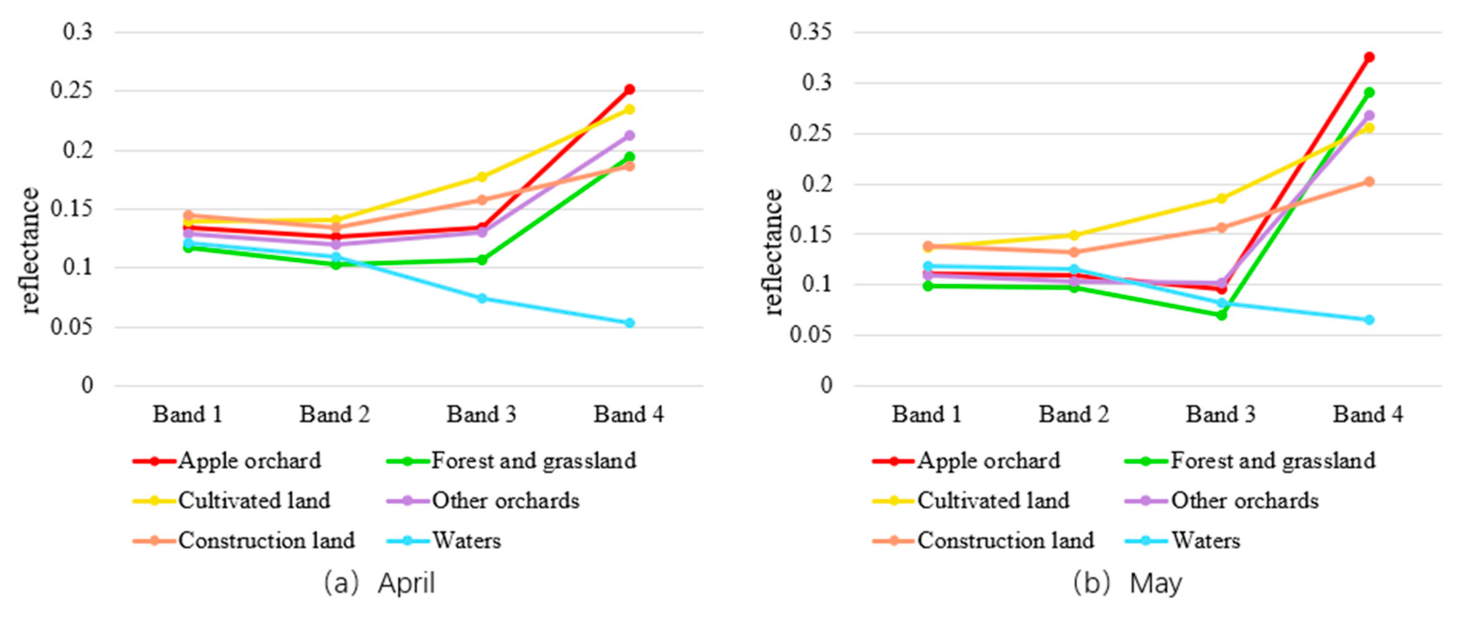
Feature Parameter Selection

Based on the characteristics of GF-6 PMS images and land cover types, brightness value, maximum spectral difference (Max. diff), mean pixel brightness value (Mean), and standard deviation of each band were selected as the feature parameters. The normalized vegetation index (NDVI), normalized water body index (NDWI), difference vegetation index (DVI), and ratio vegetation index (RVI) were selected as characteristic parameters [28,29]. To describe texture features, the gray-level co-occurrence matrix (GLCM) was used to compute eight attributes, Mean, Variance, Homogeneity, Contrast, Dissimilarity, Entropy, Angular Second Moment, and Correlation, forming the complete feature parameter combination [30] (

Table 2. Characteristic parameter.

Characteristic Exponent	Calculation Formula
NDVI	$\mathrm{N}\mathrm{D}\mathrm{V}\mathrm{I}={\displaystyle \frac{{\rho }_{\mathrm{N}\mathrm{I}\mathrm{R}}-{\rho }_{\mathrm{R}\mathrm{E}\mathrm{D}}}{{\rho }_{\mathrm{N}\mathrm{I}\mathrm{R}}+{\rho }_{\mathrm{R}\mathrm{E}\mathrm{D}}}}$
NDWI	$\mathrm{N}\mathrm{D}\mathrm{W}\mathrm{I}={\displaystyle \frac{{\rho }_{\mathrm{G}\mathrm{r}\mathrm{e}\mathrm{e}\mathrm{n}}-{\rho }_{\mathrm{N}\mathrm{I}\mathrm{R}}}{{\rho }_{\mathrm{G}\mathrm{r}\mathrm{e}\mathrm{e}\mathrm{n}}+{\rho }_{\mathrm{N}\mathrm{I}\mathrm{R}}}}$
DVI	$\mathrm{D}\mathrm{V}\mathrm{I}={\rho }_{\mathrm{N}\mathrm{I}\mathrm{R}}-{\rho }_{\mathrm{R}\mathrm{E}\mathrm{D}}$
RVI	$\mathrm{R}\mathrm{V}\mathrm{I}={\displaystyle \frac{{\rho }_{\mathrm{N}\mathrm{I}\mathrm{R}}}{{\rho }_{\mathrm{R}\mathrm{E}\mathrm{D}}}}$
Mean	$\mathrm{M}\mathrm{e}\mathrm{a}\mathrm{n}={\displaystyle \sum _{i,j=0}^{N-1}} p\left(i,j\right)\times i$
Variance	$\mathrm{V}\mathrm{a}\mathrm{r}\mathrm{i}\mathrm{a}\mathrm{n}\mathrm{c}\mathrm{e}={\displaystyle \sum _{i,j=0}^{N-1}} p\left(i,j\right)\times (i-Mean{)}^2$
Homogeneity	$\mathrm{H}\mathrm{o}\mathrm{m}\mathrm{o}\mathrm{g}\mathrm{e}\mathrm{n}\mathrm{e}\mathrm{i}\mathrm{t}\mathrm{y}={\displaystyle \sum _{i,j=0}^{N-1}} p\left(i,j\right)\times {\displaystyle \frac{1}{1+(i-j{)}^2}}$
Contrast	$\mathrm{C}\mathrm{o}\mathrm{n}\mathrm{t}\mathrm{r}\mathrm{a}\mathrm{s}\mathrm{t}={\displaystyle \sum _{i,j=0}^{N-1}} p\left(i,j\right)\times (i-j{)}^2$
Dissimilarity	$\mathrm{D}\mathrm{i}\mathrm{s}\mathrm{s}\mathrm{i}\mathrm{m}\mathrm{i}\mathrm{l}\mathrm{a}\mathrm{r}\mathrm{i}\mathrm{t}\mathrm{y}={\displaystyle \sum _{i,j=0}^{N-1}} p\left(i,j\right)\times \left|i-j\right|$
Entropy	$\mathrm{E}\mathrm{n}\mathrm{t}\mathrm{r}\mathrm{o}\mathrm{p}\mathrm{y}={\displaystyle \sum _{i,j=0}^{N-1}} p\left(i,j\right)\times \mathrm{l}\mathrm{n}\mathrm{p}\left(i,j\right)$
Angular Second Moment	$ASM={\displaystyle \sum _{i,j=0}^{N-1}} p(i,j{)}^2$
Correlation	$\mathrm{Correlation}={\displaystyle \sum _{i,j=0}^{N-1}} {\displaystyle \frac{(i-Mean)\times (j-Mean)\times p(i,j{)}^2}{Variance}}$

).

3.

Machine Learning Classifier

The K-nearest neighbor (KNN), support vector machine (SVM), and random forest (RF) algorithms were selected for apple orchard identification [31,32]. Based on the sample points measured in the field, a confusion matrix is used to verify the accuracy of the results, as shown in

Table 3. Accuracy verification.

Preliminary Classification Algorithm	UA	PA	Kappa	OA
KNN	86.08%	86.00%	0.88	87.88%
SVM	89.06%	87.86%	0.90	91.05%
RF	91.14%	90.00%	0.92	93.33%

. The random forest (RF) classification method has the highest accuracy. The user accuracy (UA) of the apple orchard is 91.14%, and the producer accuracy (PA) is 90.00%. The Kappa coefficient was 0.92, and the overall classification accuracy (OA) was 93.33%. The results of random forest identification were used as the basis for subsequent processing. The algorithm parameters for the random forest were configured as follows: the maximum depth of each tree (MaxDepth) was set to 10; the minimum number of samples required for leaf nodes (MinSampleCount) was set to 1; the maximum number of discrete feature categories (MaxCategories) was limited to 16; the regression parameter (RegressionAccuracy) was adjusted to 0.95; and the number of active features in each decision tree (ActiveVarCount) was restricted to 1.

3.2.2. Manual Annotation Data Sample Set

The complete distribution map of apple orchards in the study area was derived from the aforementioned classification result map generated by the object-oriented random forest model. Manual visual interpretation was then employed to rectify any misclassification and missing classification of the apple orchard, ensuring smooth boundary lines. During this process, two distinct labels were assigned for binarization: one denoting apple orchard areas, marked in red as shown in Figure 5, and the other representing nonapple orchard regions serving as background, marked in black in Figure 5. The original image, along with its labeled counterpart, was then uploaded onto the PIE-Engine cloud platform and divided into nonoverlapping sliding windows measuring 256 × 256 pixels each, with a consistent step size and width. Additionally, a completion setting was selected to increase reversely [33].

Using data augmentation techniques to generate diverse copies can increase the amount of valid data while preserving feature invariance, thereby aiding in mitigating overfitting issues [34]. In this study, various data augmentation methods, such as image HSV enhancement, affine transformation, flip transformation, and histogram stretching, were employed to expand the dataset (Figure 6). Consequently, a total of 7753 apple orchard image samples with a pixel size of 256 × 256 and their corresponding labeled images were obtained. The dataset was randomly divided into training and validation sets in an 8:2 ratio, resulting in 6202 images for training and 1551 images for validation. Additionally, a subset of remote sensing images from the GF-6 satellite, captured on 28 May 28 2022, was selected for further processing at a ratio of 10:1 with respect to the training set. These processed images served as the test set for evaluating the segmentation identification performance of the proposed models [35].

3.3. Enhancing of DeepLabv3+ Model

3.3.1. ResNet

To train neural network models for handling complex scenes, convolutional neural network structures are typically augmented with multiple hidden layers and a large number of weight parameters. However, as the model’s depth increases, effective training becomes increasingly challenging, resulting in limited improvements in accuracy and fitting performance [36]. To address the issues of vanishing gradient and degradation during backpropagation, ResNet introduces the concept of shortcut connection by incorporating direct connections between network layers. This allows for mapping data from one layer to another while preserving the original information from preceding layers, thereby mitigating the problem of vanishing gradient caused by an increasing number of layers [37]. Figure 7 illustrates the fundamental building block of ResNet, known as the residual unit module. Figure 7a is used for networks with fewer layers (34 layers), featuring an input channel size of 64 and a 3 × 3 convolution operation with 64 convolutional filters. In contrast, Figure 7b is used for deeper networks (50/101/152), initially employing a dimensionality reduction through a 1 × 1 convolution operation (reducing channels from 256 to 64) followed by a dimensionality increase using another 1 × 1 convolution operation (increasing channels from 64 to 256).

This study involves integrating three ResNet variant network structures, namely ResNet34, ResNet50, and ResNet101, into the DeepLabv3+ model while considering the specific conditions of training tasks and the performance of different layer structures (

Table 4. Comparison of ResNet architectures.

Component	ResNet34	ResNet50	ResNet101
Total Layers	34	50	101
Parameters	~21.8 M	~25.5 M	~44.5 M
Key Building Block	Basic Block (2 conv layers)	Bottleneck Block (3 conv layers)	Bottleneck Block (3 conv layers)
Structure Details	- 3 × 3 conv ×2 per block - No 1 × 1 conv in shortcuts	- 1 × 1 + 3 × 3 + 1 × 1 conv per block - 1 × 1 conv in shortcuts	Same as ResNet50, but with more stacked blocks
FLOPs	~3.6 GFLOPs	~4.1 GFLOPs	~7.8 GFLOPs

). Among these variants, ResNet34 is a lightweight network with a small number of parameters, making it suitable for verifying basic feature extraction capabilities. It is commonly used in lightweight comparative studies. ResNet50 employs a bottleneck architecture with moderate complexity. As the ‘gold standard’ for computer vision tasks, it balances accuracy and computational cost, making it the baseline model in most remote sensing papers [38]. The deep structure of ResNet101 serves as an effective vehicle for investigating depth-induced performance gains in analyzing high-resolution remote sensing data, where hierarchical feature extraction is crucial [39]. The strategic inclusion of these three residual networks (ResNet34/50/101) establishes a rigorous experimental framework for evaluating both computational efficiency and theoretical implications.

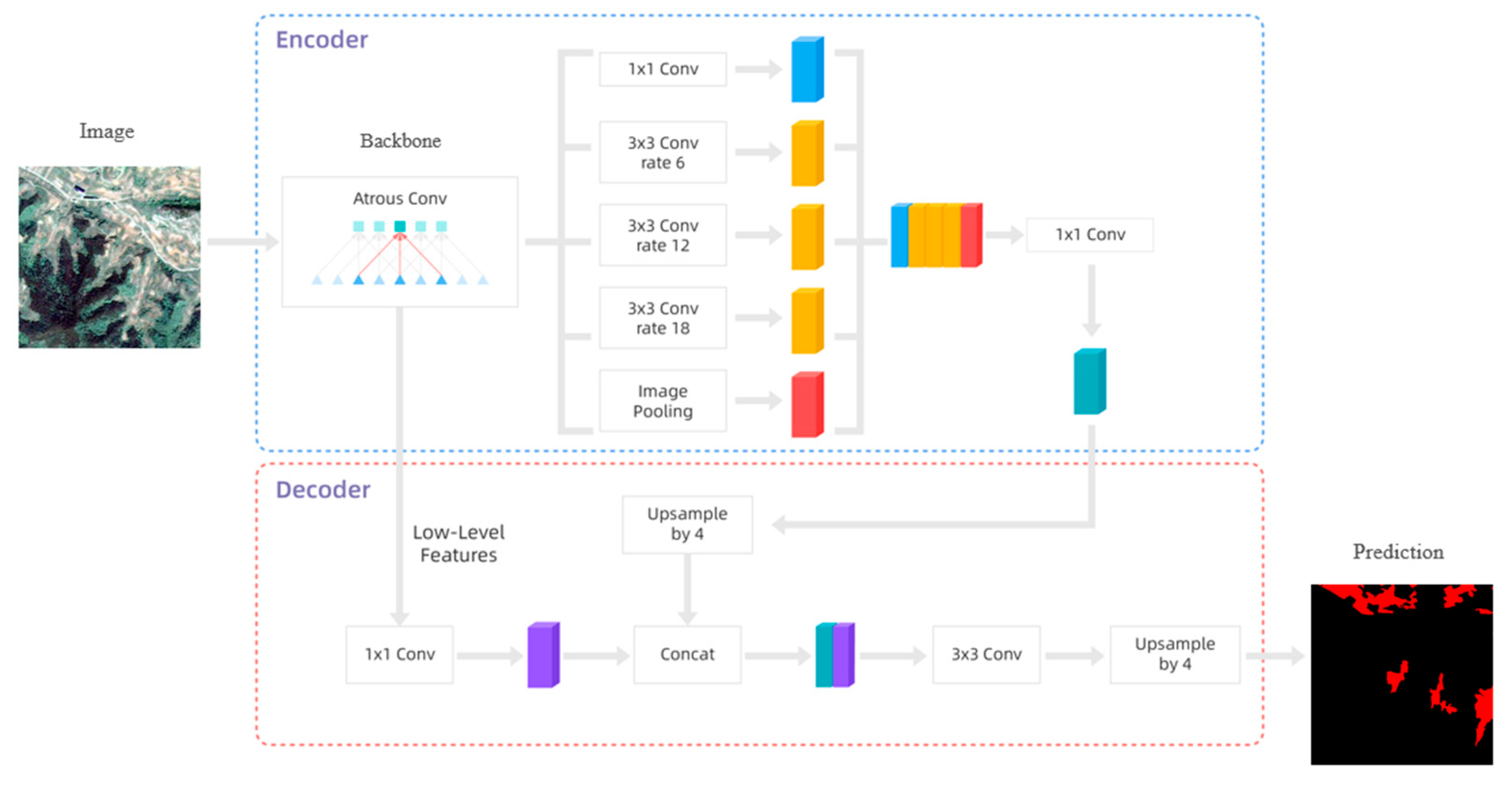
3.3.2. Construction of DeepLabv3+ Model

The DeepLabv3+ model employed in this study adopts an encoder–decoder architecture. In the encoder, convolution and pooling operations are utilized to encode positional information and image features of captured pixels. The decoder module employs deconvolution and upsampling operations to restore the size of features, effectively integrating global and local information [40,41]. To fully leverage the multispectral information in the GF-6 PMS image, enhancements are made to the input layer and data reading mode of the DeepLabv3+ model, enabling it to process data from four channels. By employing a 1 × 1 convolutional layer and average pooling strategy, semantic segmentation tasks can be performed on images of arbitrary sizes without being limited by fixed input dimensions. ResNet34, ResNet50, and ResNet101 residual networks are introduced to enhance the original backbone network module, resulting in three network models: DeepLabv3+_34, DeepLabv3+_50, and DeepLabv3+_101.

In the semantic segmentation task of convolutional neural networks, the downsampling operation can lead to significant loss of spatial information in images. However, by using dilated convolution with different dilation rates to capture information at various scales, the spatial resolution of images can be maintained while increasing the receptive field [42,43]. Combining dilated convolution with Atrous Spatial Pyramid Pooling (ASPP) forms an effective structure for extracting multiscale feature information. This approach includes dilated convolution and pooling operations at different sampling rates, which can obtain receptive fields of various scales and rich contextual information, enhancing the network’s ability to identify objects of different scales [44]. The multiscale pooling operation helps avoid the information loss typically caused by traditional pooling while preserving spatial resolution, thereby improving the network performance. Using different convolution kernel sizes allows the network to capture diverse feature information and enhances its nonlinear capability.

This model also incorporates deep supervision technology by incorporating loss functions into decoders at different levels, enabling low-level features to participate in the supervision process. This integration facilitates better utilization of multiscale information and enhances the model’s performance. The structure of the DeepLabv3+ network is illustrated in Figure 8. The term ‘Encoder’ refers to the encoding stage, where the “Backbone” denotes the backbone network. In this research model, three architectures—ResNet34, ResNet50, and ResNet101—are utilized for replacement. The network performance is enhanced through the residual connections, which benefits deep neural networks and training efficiency. Upon inputting an image into the network, the ‘Backbone’ component first extracts features from the remote sensing image, resulting in low-level and high-level feature maps. The high-level feature map is then fed into the ‘Atrous Conv’ module, which employs dilated convolutions under a pyramid structure. Specifically, this module introduces a dilation rate in each convolution kernel and conducts dilated convolution and pooling operations at various sampling rates, allowing the model to capture multiscale features effectively. Finally, feature fusion is performed on all the feature outputs generated by the pyramid, and the final feature map in the encoding stage is obtained after applying a 1 × 1 convolution. The ‘Decoder’ corresponds to the decoding stage, where ‘Upsample by 4′ indicates that the high-level feature map is upsampled four times. The ‘Concat’ module concatenates the low-level features generated by the backbone and the high-level features obtained in the encoding phase, followed by a 3 × 3 convolution layer and an additional four times upsampling to restore the original image size and yield the final prediction.

3.3.3. Model Enhancement

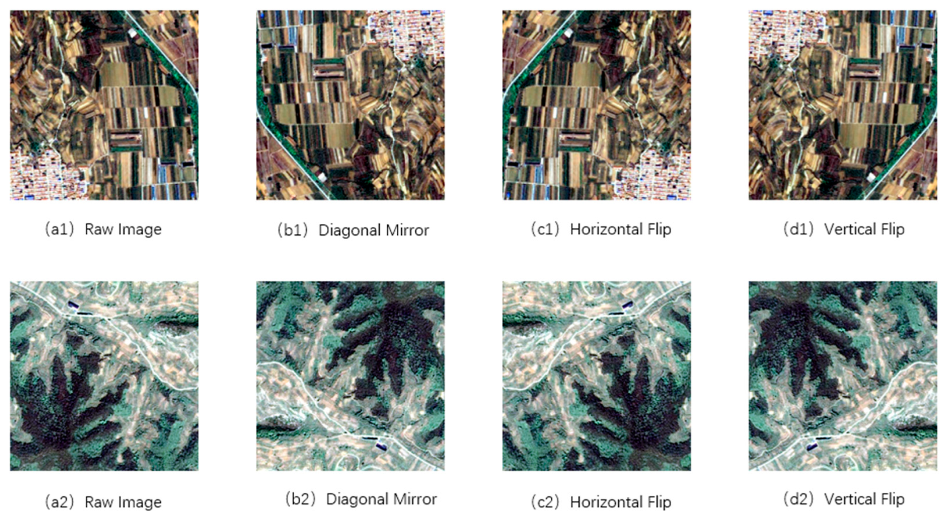
The optimization algorithm of the neural network significantly affects the model’s update trajectory in the parameter space, thereby influencing both convergence speed and stability, ultimately enhancing model performance [45,46]. In this study, the hybrid loss method was employed as the chosen optimization algorithm for calculating pixel-level network structure loss. The hybrid loss function mainly consists of the following components:

(1)

Cross-Entropy: The minimum cross-entropy is equivalent to minimizing the relative entropy between the actual output and the expected output, which can be measured by calculating the KL divergence of probability distributions $p$ and $q$. Formula 1 presents the definition of cross-entropy when considering two discrete probability distributions.

$$L\left(\theta \right)=H\left(p,q\right)=-\sum _x p\left(x\right)\log q\left(x\right)$$

(1)

(2)

Dice Loss: It is utilized for quantifying the similarity between the predicted outcome and the actual label, exhibiting a high sensitivity towards object boundary accuracy.

$$Loss=1-{\displaystyle \frac{2\left|X\cap Y\right|}{\left|X\right|+\left|Y\right|}}$$

(2)

where $\left|\mathrm{X}\cap \mathrm{Y}\right|$ represents the intersection of X and Y samples. The numerator has a coefficient of 2 because the denominator actually counts the intersection twice.

Then, the adaptive moment estimation (Adam) gradient descent optimization algorithm was employed to dynamically adjust the learning rate. This algorithm updates the parameters based on estimates of the first and second moments of the parameter gradient, enabling adaptive changes in the learning rate with varying parameters.

$$\left\{\begin{array}{c}{m}_t={\beta }_1{m}_{t-1}+(1-{\beta }_1)\Delta L\left(\theta \right)\\ {\nu }_t={\beta }_2{\nu }_{t-1}+(1-{\beta }_2)\Delta L(\theta {)}^2\end{array}\right.$$

(3)

where $m$ represents the first-order matrix estimate of the parameter gradient, $t$ indicates the number of current iterations, ${\beta }_1$ is the coefficient for the first-order matrix estimate of the parameter gradient with a value in range [0, 1], $\nu$ is the second-order matrix estimate of the parameter gradient, and ${\beta }_2$ is the coefficient for the second-order matrix estimate of the parameter gradients with a value in range [0, 1].

In the Adam algorithm, both $m$ and $\nu$ were initialized as vector 0; thus, the deviations of $m_t$ and ${\nu }_t$ were corrected seperately, as shown in Formula 4:

$$\left\{\begin{array}{c}{m}_t^{\prime }={\displaystyle \frac{m_t}{1-{\beta }_1^t}}\\ {\nu }_t^{\prime }={\displaystyle \frac{{\nu }_t}{1-{\beta }_2^t}}\end{array}\right.$$

(4)

If the unbiased first-order matrix estimate and the unbiased second-order matrix estimate of the parameter gradient are known, the parameter update of Adam is shown in Formula 5:

$${\theta }_{t+1}={\theta }_t-{\displaystyle \frac{\eta }{\sqrt{{\nu }_t^{\prime }}+\epsilon }}\otimes m_t^{\prime }$$

(5)

The Adam algorithm combines the benefits of both momentum stochastic gradient descent and adaptive gradient descent while incorporating correction factors in the computation of first-order and second-order matrices estimates. This results in faster convergence speeds and effectively addresses issues arising from excessive or sparse gradient noise [47].

The learning rate schedule chosen is the multistep dynamic adjustment of learning rate (MultiStepLR). This schedule involves specifying the number of decay steps and decay factor, while monitoring the current iteration number (epoch) during training. When the current epoch reaches a specified milestone, the learning rate is adjusted by multiplying it with the decay factor. Here, milestones refer to user-defined decay steps, and gamma represents the multiplier for the decay factor.

3.3.4. Hyperparameter Configuration

The setting of hyperparameters plays a crucial role in the performance and training effect of the model [48]. The deep learning in this study runs on Windows10 using NVIDIA (Santa Clara, CA, USA) T4 Tensor Core GPUs provided by the PIE-Engine cloud platform. In terms of CPU, the AMD (Sunnyvale, CA, USA) Ryzen 7 4800H is equipped with eight physical cores and 16 logical processors at a base frequency of 2900 Mhz. PyTorch1.2 deep learning framework was used to build the network, and the software environment was Anaconda (Python 3.11).

The initial learning rate for model training was set to 0.003, and the batch size was configured at 10. For performance evaluation, test set images were selected at a ratio of 10:1 to the number of training set images within each batch. Due to computational limitations, each training session consisted of 300 epochs, followed by repeated rounds of iterative training based on the previous model. Early stopping was employed to monitor the loss value of the validation set and determine when to terminate the model to prevent overfitting. A hybrid loss function was chosen, and an Adam optimizer with an adaptive learning rate gradient descent algorithm was utilized. The coefficient betas for calculating running averages of gradients and gradient squares were set as [0.9, 0.999], while the epsilon value for numerical stability enhancement was defined as 1 × 10⁻⁸. The learning rate decay strategy adopted the MultiStepLR approach, with milestones at epochs [35,45], where the learning rate is adjusted after reaching these specific epochs using a gamma value of 0.1.

3.4. Model Performance Evaluation

The confusion matrix is utilized to assess the accuracy of different models in classifying apple orchards. TP (True Positive) indicates that the sample is correctly classified as positive by the model. FP (False Positive) represents a false positive example, where the sample is actually negative but predicted as positive by the model. FN (False Negative) denotes a false negative example, where the sample is actually positive but predicted as negative by the model. TN (True Negative) signifies a true negative example, where both the actual and predicted values are negative. The specific performance indicators can be calculated using the following formulas:

(1)

Precision:

$$Precision={\displaystyle \frac{TP}{TP+FP}}$$

(6)

(2)

Recall:

$$Recall={\displaystyle \frac{TP}{TP+FN}}$$

(7)

(3)

Intersection over Union (IoU):

$$IoU={\displaystyle \frac{p_{ii}}{\sum _{j=0}^k p_{ij}+\sum _{j=0}^k p_{ji}-p_{ii}}}$$

(8)

where $p_{ii}$ represents the quantity marked as Category $i$ in Category $i$ data, $p_{ij}$ represents the quantity marked as Category $j$ in Category $i$ data, and $p_{ji}$ represents the quantity marked as Category $i$ in Category $j$ data.

(4)

Mean Intersection over Union (mIoU):

$$MIoU={\displaystyle \frac{1}{k+1}}\sum _{i=0}^k {\displaystyle \frac{p_{ii}}{\sum _{j=0}^k p_{ij}+\sum _{j=0}^k p_{ji}-p_{ii}}}$$

(9)

4. Results

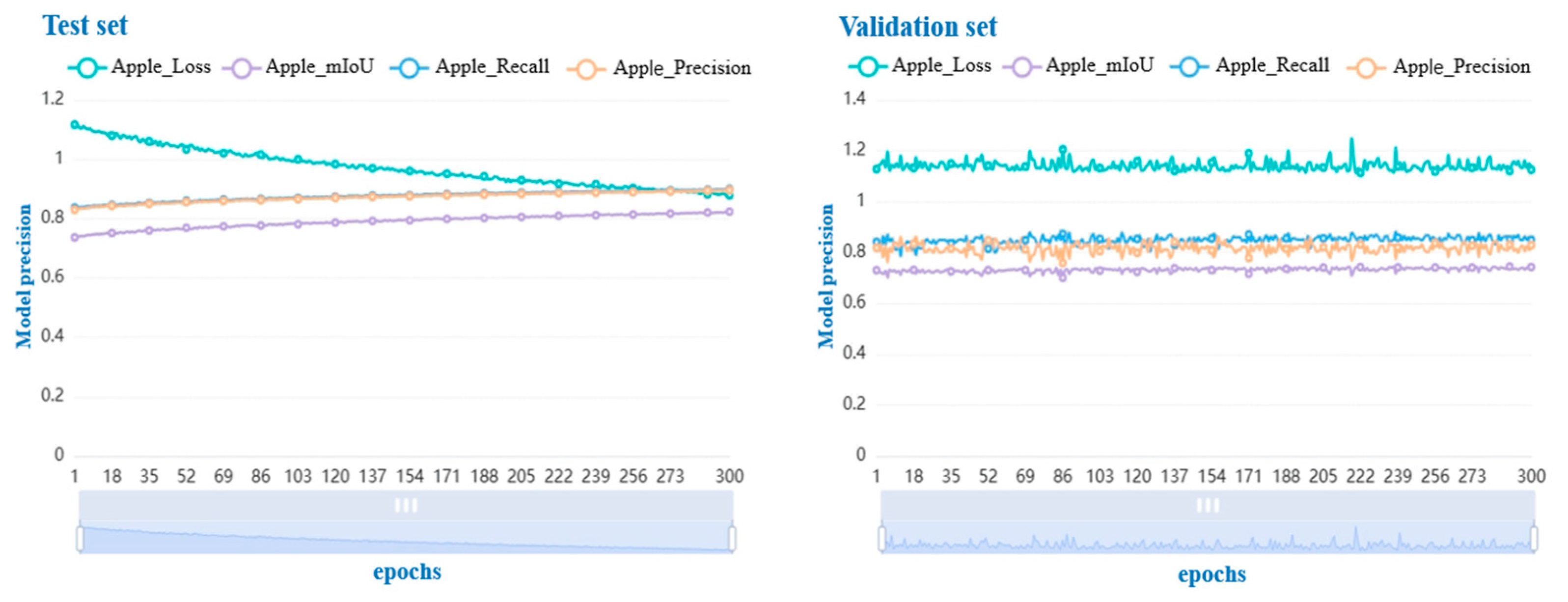
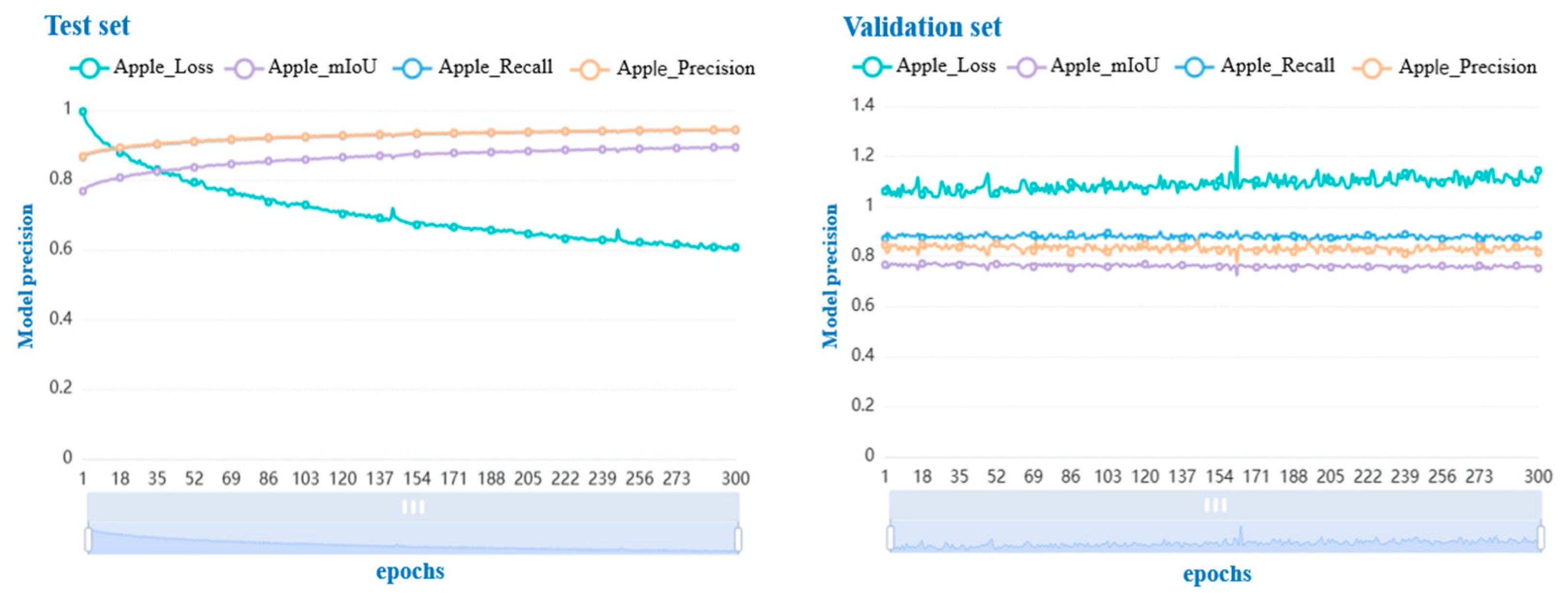
4.1. Enhanced Model Training Results

The three models (DeepLabv3+_34, DeepLabv3+_50, and DeepLabv3+_101) constructed in this study all employed the approach of training for 300 epochs in a single session and multiple rounds of iterative training based on the previous model. Figure 9, Figure 10 and Figure 11, respectively, depict the change curves of various performance evaluation metrics for the test set and validation set after three iterations of training for each model. The horizontal axis represents epochs, while the vertical axis represents the accuracy value of apple orchard segmentation identification for each batch during model training. The green curve illustrates the trend in model loss, the purple curve represents mIoU values for apple orchard identification results, and the blue curve corresponds to recall values for apple orchard, which closely aligns with the orange curve indicating changes in precision values.

After reaching 300 epochs in the third iteration experiment and a total of 900 epochs, the training loss of the DeepLabv3+_34, DeepLabv3+_50, and DeepLabv3+_101 models exhibited convergence tendencies, with each precision value reaching its peak during iterative training. The DeepLabv3+_34 model achieved a Precision of 91.17%, a Recall of 91.40%, and an mIoU of 84.67%. The DeepLabv3+_50 model achieved a Precision of 92.55%, a Recall of 92.70%, and an mIoU of 86.79%. As for the DeepLabv3+_101 model, it obtained Precision, Recall, and mIoU values of 94.37%, 94.27%, and 89.33%, respectively.

4.2. Analysis of the Ablation Experiment Results

The ablation experiment, employing the control variable method, validated the enhanced performance of the optimization module for model identification while maintaining consistent environmental conditions and parameter configurations. ResU-Net and LinkNet represent classical architectures in semantic segmentation, both building upon the foundational U-Net framework with distinct structural modifications. To systematically evaluate both the performance of the DeepLabv3+ architecture and the optimization effects of different ResNet backbone structures, in this study, various models, including DeepLabv3+_34, DeepLabv3+_50, DeepLabv3+_101, ResU-Net, and LinkNet, were trained on GF-6 PMS training set images under identical environmental configuration settings. Two 4-band NIR-R-G-B GF-6 PMS satellite remote sensing images from the test set were selected to conduct remote sensing identification of apple orchard within mixed scenes comprising water bodies, urban areas, forest and grassland, and farmlands. Qualitative and quantitative analysis was performed on the identification results obtained by different models to ascertain the extent of network model optimization through ResNets at different layers and compare the performance advantages of DeepLabv3+ model against common semantic segmentation models. The predicted apple orchard area identified by the semantic segmentation model in each image is highlighted in red, while nonapple orchard areas are marked in black as background.

Compared with the identification results of ResNet models with different layers, the DeepLabv3+_34, DeepLabv3+_50, and DeepLabv3+_101 semantic segmentation models exhibited no missing points in the apple orchard and accurately identified the complete distribution of the apple orchard without any gaps within the garden. However, both DeepLabv3+_34 and DeepLabv3+_50 models had limited capability in handling complex backgrounds and multiscale information. These models tended to misclassify vegetated areas such as forests and grasslands as an apple orchard. On the other hand, the DeepLabv3+_101 model exceled at identifying thin linear roads with smooth segmentation edges and performs better when dealing with complex backgrounds (Figure 12). While ResNet34 and ResNet50 had relatively shallow layers, resulting in faster training speed along with lower memory and computing resource requirements, ResNet101 offered greater expressiveness by enabling learning and extraction of more complex features. It also demonstrated superior performance on large datasets or tasks that demanded high precision.

Compared with the identification results of ResU-Net and LinkNet models, which also incorporate the ResNet, the enhanced DeepLabv3+ model utilizes the ASPP module to effectively capture context information at various scales. This led to a significant increase in sensitivity field and enables the processing of multiscale images. Additionally, deep supervision technology was employed in the enhanced DeepLabv3+ model, allowing low-level features to participate in supervision and facilitating better integration of multiscale information. Moreover, this enhanced model exhibited superior accuracy in identifying apple orchard distributions without missing any points. The resulting edges were relatively smooth and neat, while other ground objects were well segmented into black-marked background areas (Figure 13).

Table 5. Experiment results of different models on the test dataset.

Model	Precision/%	Recall/%	mIoU/%
ResU-Net34	86.55%	86.98%	80.87%
ResU-Net50	89.48%	89.82%	82.20%
ResU-Net101	90.82%	90.69%	83.23%
LinkNet34	88.46%	88.13%	82.96%
LinkNet50	92.48%	91.87%	86.71%
LinkNet101	92.52%	92.19%	85.92%
DeepLabv3+_34	91.17%	91.40%	84.67%
DeepLabv3+_50	92.55%	92.70%	86.79%
DeepLabv3+_101	94.37%	94.27%	89.33%

presents the apple orchard identification accuracy of different semantic segmentation algorithm models on the test set images. Notably, the Precision score for the DeepLabv3+_101 model reached an impressive 94.37%.

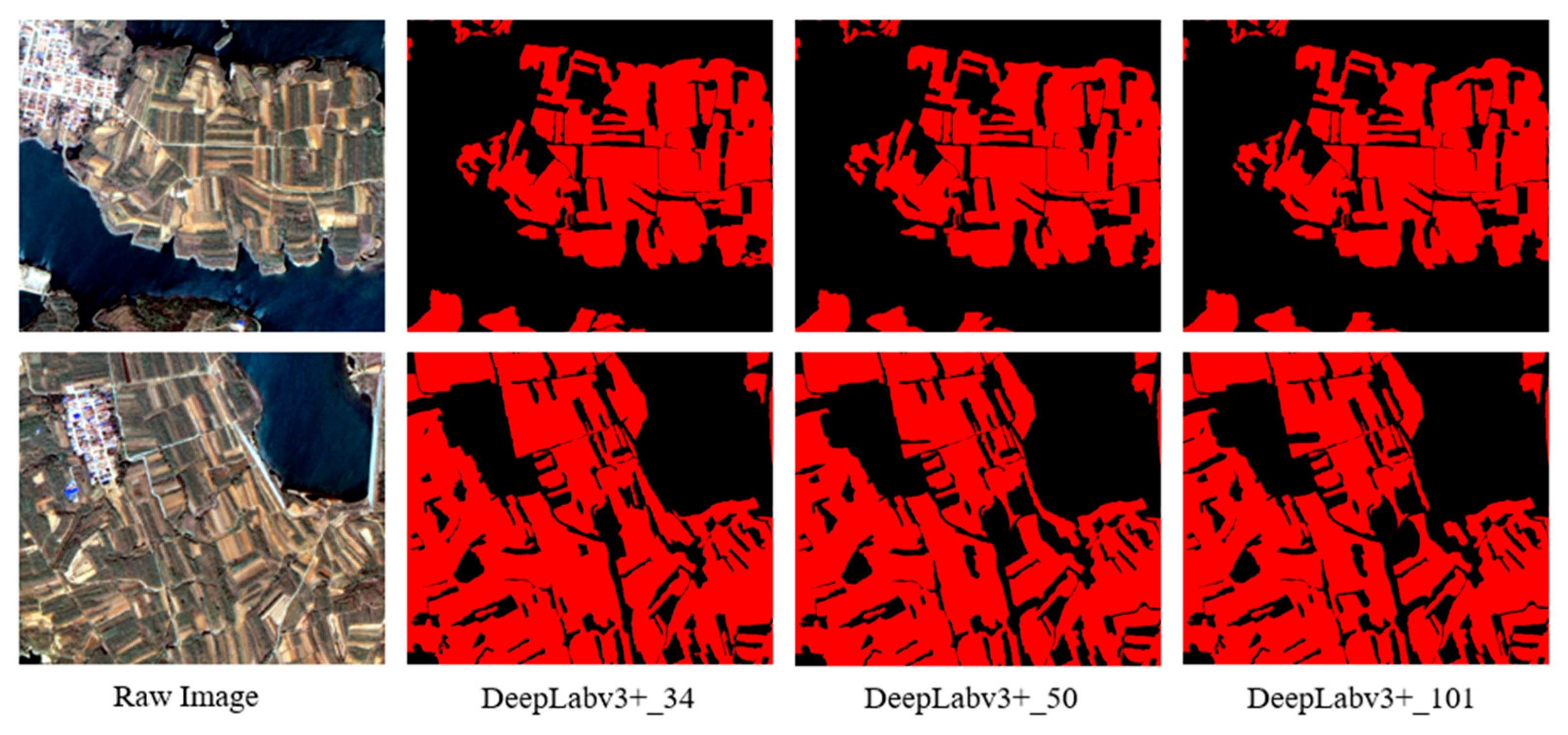
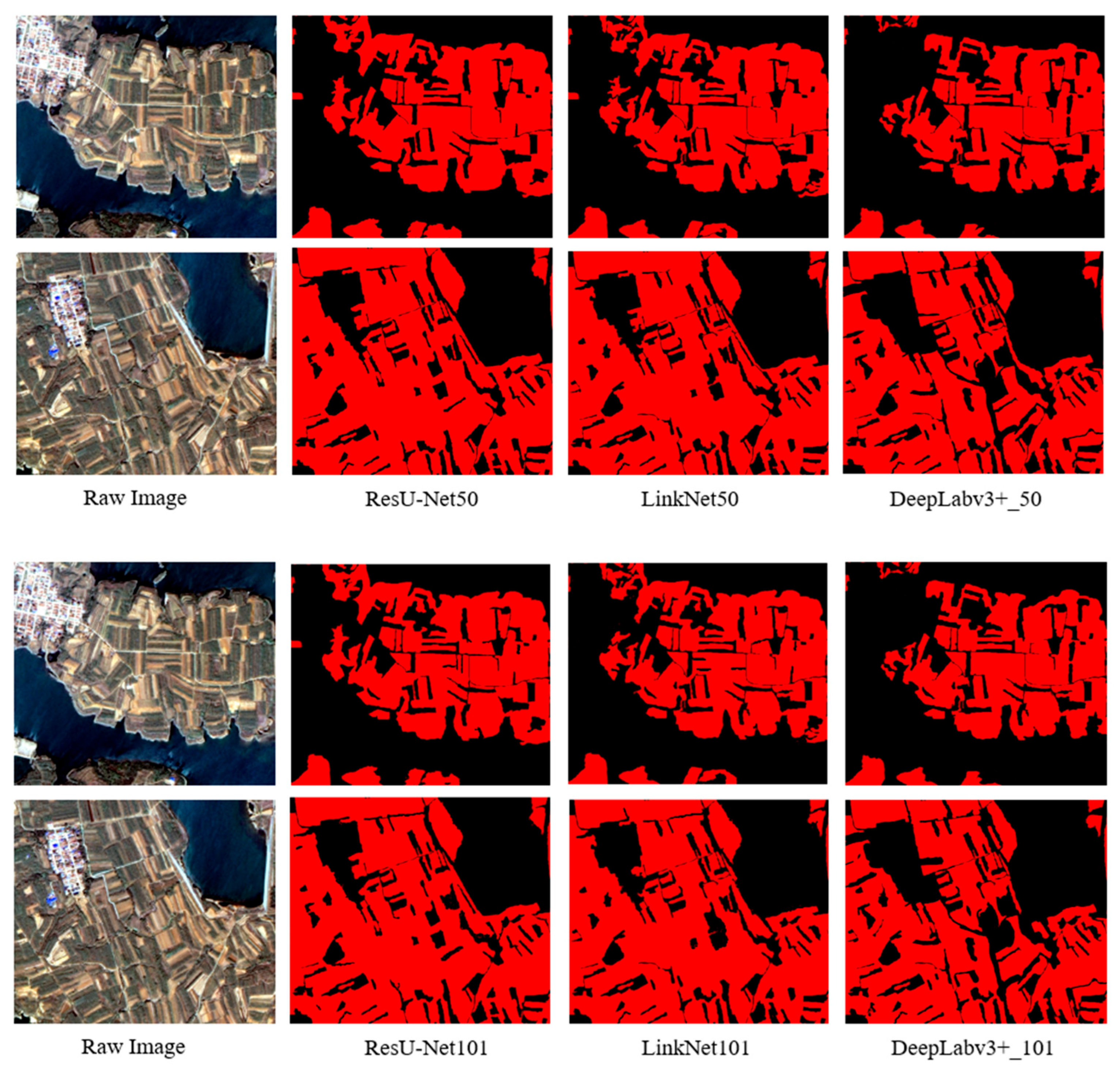
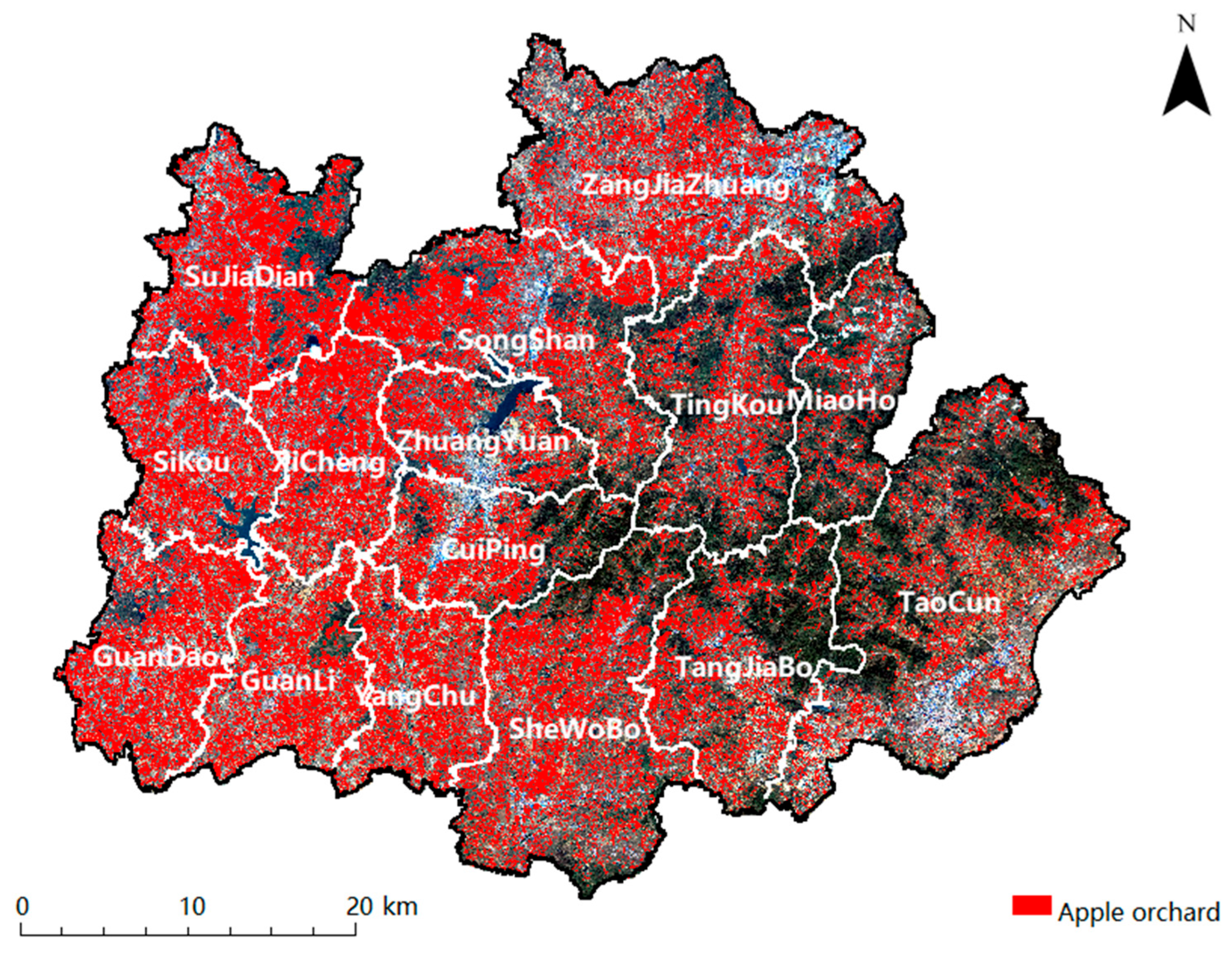
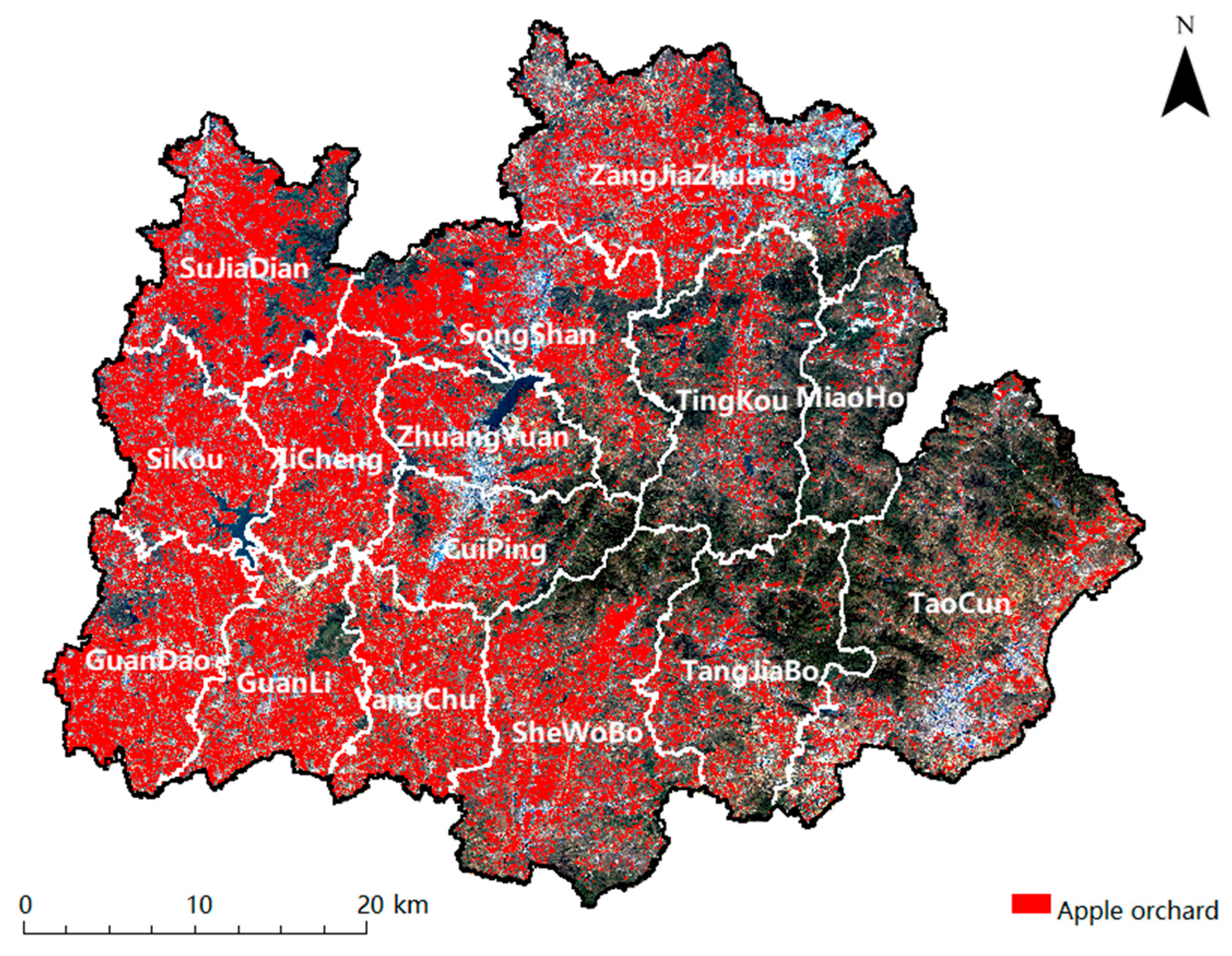
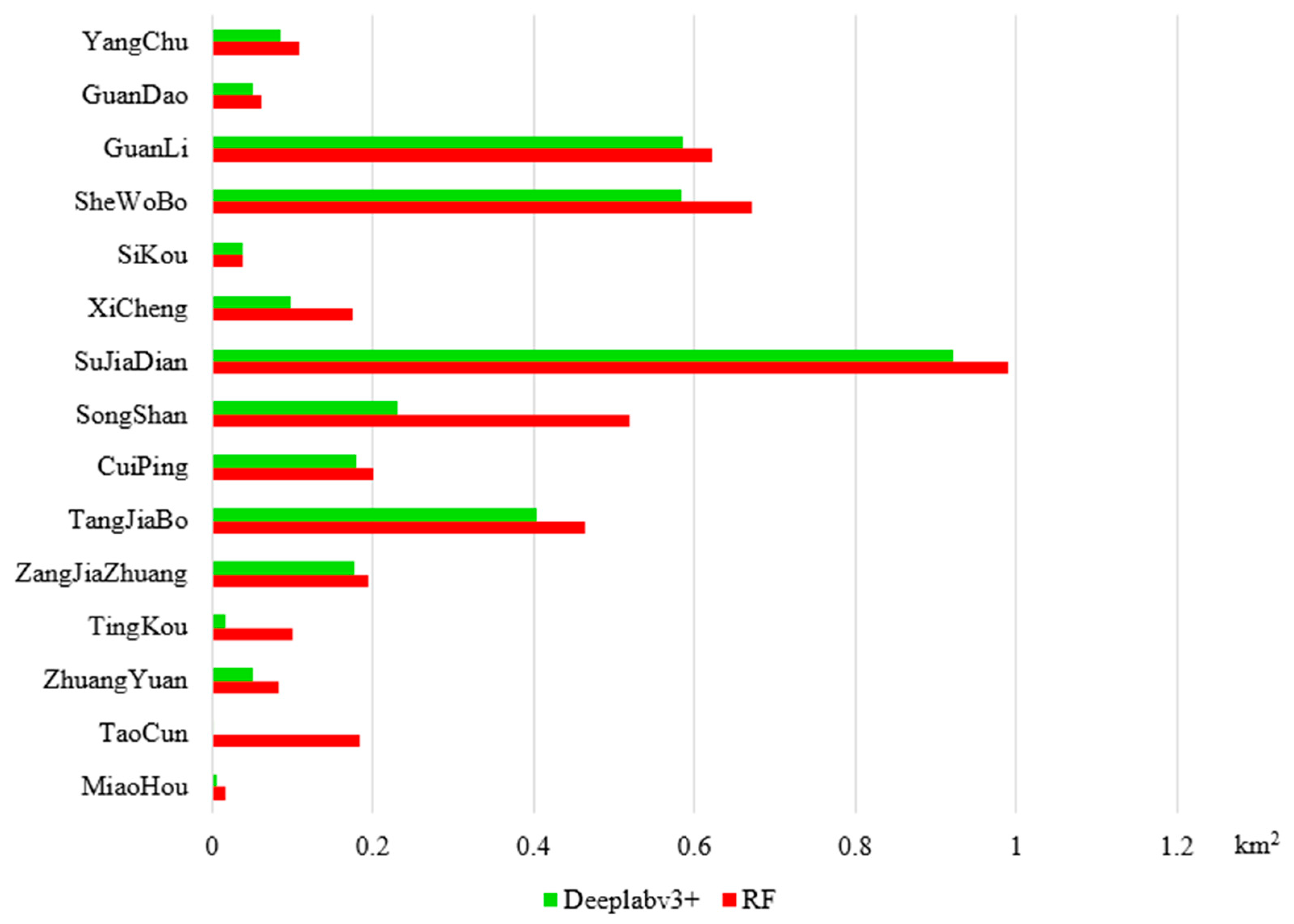
4.3. Comparison of Identification Results

The distribution maps of the apple orchard identified by the object-oriented+random forest algorithm and DeepLabv3+_101 model, respectively, are presented in Figure 14 and Figure 15. The comparison results reveal a generally consistent spatial distribution pattern of apple orchards in both datasets. Apple orchards were predominantly located in western areas of the study area, including Guandao Town, Guanli Town, Yangchu Town, Sikou Town, Xicheng Town, and Shewobo Town. However, there was a relatively sparse distribution of apple orchards in Miaohou Town and Taocun Town, situated in the eastern part of the study area. Nevertheless, it should be noted that misclassification occurred with regard to identifying apple orchards using the object-oriented+random forest algorithm. In certain areas, such as Tingkou Town, Tangjiapo Town, Miaohou Town, and Taocun Town, the algorithm incorrectly labeled some forest and grassland and other orchard types as apple orchards (Figure 15). To facilitate comparison, one village was randomly selected in each town to count and compare the apple orchard area identified by the two algorithm models (Figure 16). The vertical coordinate represented the township, while the horizontal coordinate was the apple orchard area (km²) counted by both algorithm models. The DeepLabv3+_101 model demonstrated higher accuracy when identifying and distributing apple orchards within the study area.

According to the official field measurement results of Qixia City in 2023, apple orchards covered an area of 666.66 km². This study calculated the overall area of the apple orchard distribution map identified by the DeepLabv3+_101 model and the random forest classification algorithm. The random forest classification algorithm identified an area of 723.41 km² with an accuracy rate of 91.49%, but it tended to overestimate the actual extent. DeepLabv3+_101 model recognized an area of 629.32 km² with a high accuracy rate of 94.40%. This accounts for approximately 31.20% of the study area’s total land area and aligns closely with official data, even though there is a tendency to underestimate its true magnitude compared with the official data.

Calculating the proportion of apple orchard planting areas within each town’s geographical boundaries can provide insights into regional preferences for such cultivation and offer valuable information about agricultural economy proportions. Among them, the apple orchard areas in Guandao Town, Guanli Town, Yangchu Town, Sikou Town, Xicheng Town, and Shewobo Town accounted for over 40% of their respective areas, indicating that these towns place great importance on and rely heavily on the apple industry. Conversely, although the apple planting areas in Sujiadian Town, Songshan sub-district, Zhuangyuan sub-district, Cuiping sub-district, Tangjiapo Town, Zangjiazhuang Town, and Tingkou Town were smaller than those previously mentioned, they still accounted for more than 20% of each town’s total area, suggesting that the apple industry also plays a significant role in these towns. In general, the apple industry is not only the agricultural pillar of Guandao Town and other towns but also occupies an important position in Sujiadian Town and other towns and has made important contributions to the development of the local agricultural economy. The distribution of apple orchards in the central and eastern regions was sparse, and the apple orchards in Miaohou Town and Taocun Town in the eastern townships had the lowest proportion, accounting for about 12% of the township area (

Table 6. The distribution of apple orchard areas in each township based on DeepLabv3+ recognition.

Township	Area of Apple Orchard (km2)	Township Area (km2)	Apple Orchard Area Proportion (%)
YangChu	47.58	86.76	54.84
GuanDao	55.95	113.47	49.31
GuanLi	46.92	97.44	48.15
SheWoBo	92.03	201.69	45.63
SiKou	40.82	91.60	44.56
XiCheng	44.75	91.27	49.03
SuJiaDian	48.36	136.43	35.45
SongShan	45.34	158.50	28.61
CuiPing	23.97	89.74	26.71
TangJiaBo	28.83	138.69	20.79
ZangJiaZhuang	55.96	223.14	25.08
TingKou	32.39	151.30	21.41
ZhuangYuan	20.63	73.80	27.95
TaoCun	35.12	277.56	12.65
MiaoHou	10.67	85.27	12.51
Total	629.32	2016.66	31.21

).

5. Discussions

The innovation of this research lies in the utilization of a combination of image annotation and object-oriented methods during the training process of the semantic segmentation model, enhancing both efficiency and accuracy in manual annotation. Additionally, an improved DeepLabv3+ model was constructed based on GF-6 satellite images, exhibiting superior performance in feature expression compared with traditional machine learning classification and recognition algorithms.

The establishment of a deep learning semantic segmentation model necessitates a substantial amount of labeled data for initial training [49]. Particularly in cases where the study area is extensive and complex in land cover types, manual labeling becomes an arduous task, thereby increasing the technological and computational challenges to some extent [50]. In this study, object-oriented technology was employed along with multiscale segmentation of satellite images to first obtain a distribution map of apple orchards using the RF classification method. This result was then supplemented by manual correction to construct label images that matched the original image’s size, which were subsequently segmented to generate a sample dataset. By simplifying the laborious process of manual labeling and ensuring consistency across the entire scene image through labeling a wide range of satellite image samples, this approach avoids potential drawbacks associated with traditional cutting labeling methods that may result in loss of overall context information.

Machine learning algorithms for land cover classification typically rely on complex feature parameter extraction techniques. The layer procedures require expert domain knowledge and manual design, while the resulting algorithm model is specific to a particular research area with limited universality in terms of feature parameter combinations. Yan et al. [51] achieved 90% identification accuracy for apple orchards using multitemporal Sentinel-2 imagery and Random Forest (RF) classification. In this study, the proposed model combining DeepLabv3+ and ResNet101 achieved a precision of 94.37%, which was 3.23% higher than that of object-oriented and random forest identification. Compared with the object-oriented classification algorithm combined with machine learning used in this study, the proposed approach automatically learns feature representations without manual design, demonstrating excellent performance in processing complex scenes and multicategory classification. The identified ground objects exhibited refined details, smoother edges, and better generalization ability. Mpakairi et al. [52] conducted a comparative study on farmland recognition using deep learning and traditional machine learning and reached conclusions consistent with ours. The CNN framework allows for progressive iteration and upgrading, with its inherent scalability for large datasets effectively offsetting the preliminary computational costs.

By inputting all the band information in the multispectral image into the model, the discrepancy between pixel values can address the issue of similar texture characteristics between other regions and apple orchards. Previous semantic segmentation models based on convolutional neural networks mostly utilized R-G-B images for training data, resulting in limited identification accuracy. For example, Zhang et al. [53] used drone RGB imagery combined with LinkNet to identify apple orchards on the Loess Plateau but did not fully investigate the impact of near-infrared bands on crops. In this study, enhancements were made to the network’s input layer and data reading mode to enable it to process data from four channels, leading to the construction of a semantic segmentation model trained on a 4-band NIR-R-G-B image. The inclusion of a near-infrared band synthesizes additional spectral information and approximates real-world outcomes more closely, effectively mitigating interference from texture features and enhancing vegetation differentiation. To handle complex tasks encountered in this study’s intricate scenario, incorporating the ResNet101 structure as part of the model backbone network improves its capability while avoiding potential issues such as gradient disappearance and degradation during training.

There are limitations in this study. This study selected Qixia City, the apple capital of China, as the case study area, and constructed and validated a classification model with the GF-6 image of the key growth period in May. Future studies will select more typical areas and examine the proposed method for longer growing periods of apple trees. Besides, GF-6 images were used in this study as the primary data source for precise identification of apple orchards; however, the GF-6 image has a limited temporal coverage (2018 to present), which limits the scope of application of the recognition model proposed in this study. More work will be conducted to explore the fusion method of GF-6 with multimodal images over a long temporal coverage scope to enrich the image details of the study area and improve the long-term monitoring capability. Furthermore, the method proposed in this study has the potential for further improvement. Integrating attention mechanisms into the network structure during feature extraction can enhance meaningful features in images while suppressing irrelevant ones, further improving training accuracy and enabling efficient extraction of challenging ground objects such as apple orchards, which will be the direction of future research endeavors.

6. Conclusions

The enhanced DeepLabv3+ semantic segmentation remote sensing identification model for apple orchard in this study achieved accurate identification of apple orchard, thereby improving identification accuracy compared with conventional machine learning classification and identification methods. The research results show that the accuracy of apple orchard extraction based on the enhanced DeepLabv3+ model was 94.37%, the recall was 94.27%, and the mIoU was 89.33%. The proposed method achieved 94% accuracy in apple orchard area identification across Qixia City, demonstrating a statistically significant 3-percentage-point improvement over the random forest (RF) approach (91% accuracy). The identification effect of the enhanced DeepLabv3+ model was significantly higher than that of the ResU-Net and LinkNet models. The enhanced DeepLabv3+ model has excellent performance in processing complex scenes and multicategory classification, which can accurately monitor the spatial pattern of apple orchards, surpassing the accuracy and efficiency of conventional machine learning classification algorithms. The findings of this study can provide valuable reference for the application of convolutional neural networks in cash crop identification.

References

1. Na, W.; Wolf, J.; Zhang, F.S. Towards sustainable intensification of apple production in China—Yield gaps and nutrient use efficiency in apple farming systems. J. Integr. Agric. 2016, 15, 716–725. [Google Scholar]
2. Zhou, H.; Niu, X.; Yan, H.; Zhao, N.; Zhang, F.; Wu, L.; Yin, D.; Kjelgren, R. Interactive effects of water and fertilizer on yield, soil water and nitrate dynamics of young apple tree in semiarid region of northwest China. Agronomy 2019, 9, 360. [Google Scholar] [CrossRef]
3. Frolking, S.; Qiu, J.; Boles, S.; Xiao, X.; Liu, J.; Zhuang, Y.; Li, C.; Qin, X. Combining remote sensing and ground census data to develop new maps of the distribution of rice agriculture in China. Glob. Biogeochem. Cycles 2002, 16, 38-1–38-10. [Google Scholar] [CrossRef]
4. Zhang, C.; Valente, J.; Kooistra, L.; Guo, L.; Wang, W. Orchard management with small unmanned aerial vehicles: A survey of sensing and analysis approaches. Precis. Agric. 2021, 22, 2007–2052. [Google Scholar] [CrossRef]
5. Ballesteros, R.; Ortega, J.F.; Hernandez, D.; Del Campo, A.; Moreno, M.A. Combined use of agro-climatic and very high-resolution remote sensing information for crop monitoring. Int. J. Appl. Earth Obs. 2018, 72, 66–75. [Google Scholar] [CrossRef]
6. Berni, J.A.; Zarco-Tejada, P.J.; Suárez, L.; Fereres, E. Thermal and narrowband multispectral remote sensing for vegetation monitoring from an unmanned aerial vehicle. IEEE Trans. Geosci. Remote 2009, 47, 722–738. [Google Scholar] [CrossRef]
7. Xia, T.; He, Z.; Cai, Z.; Wang, C.; Wang, W.; Wang, J.; Hu, Q.; Song, Q. Exploring the potential of Chinese GF-6 images for crop mapping in regions with complex agricultural landscapes. Int. J. Appl. Earth Obs. 2022, 107, 102702. [Google Scholar] [CrossRef]
8. Chen, K.; Chen, B.; Liu, C.; Li, W.; Zou, Z.; Shi, Z. Rsmamba: Remote sensing image classification with state space model. IEEE Geosci. Remote Sens. Lett. 2024, 21, 8002605. [Google Scholar] [CrossRef]
9. Coulibaly, S.; Kamsu-Foguem, B.; Kamissoko, D.; Traore, D. Deep learning for precision agriculture: A bibliometric analysis. Intell. Syst. Appl. 2022, 16, 200102. [Google Scholar] [CrossRef]
10. Zhang, D.; Pan, Y.; Zhang, J.; Hu, T.; Zhao, J.; Li, N.; Chen, Q. A generalized approach based on convolutional neural networks for large area cropland mapping at very high resolution. Remote Sens. Environ. 2020, 247, 111912. [Google Scholar] [CrossRef]
11. Kamilaris, A.; Prenafeta-Boldú, F.X. Deep learning in agriculture: A survey. Comput. Electron. Agric. 2018, 147, 70–90. [Google Scholar] [CrossRef]
12. Comba, L.; Gay, P.; Primicerio, J.; Aimonino, D.R. Vineyard detection from unmanned aerial systems images. Comput. Electron. Agric. 2015, 114, 78–87. [Google Scholar] [CrossRef]
13. Sun, Z.; Zhu, S.; Gao, Z.; Gu, M.; Zhang, G.; Zhang, H. Recognition of grape growing areas in multispectral images based on band enhanced DeepLabv3+. Trans. CSAE 2022, 38, 229–236. [Google Scholar]
14. Chen, R.; Zhang, C.; Xu, B.; Zhu, Y.; Zhao, F.; Han, S.; Yang, G.; Yang, H. Predicting individual apple tree yield using UAV multi-source remote sensing data and ensemble learning. Comput. Electron. Agric. 2022, 201, 107275. [Google Scholar] [CrossRef]
15. Hung, C.; Xu, Z.; Sukkarieh, S. Feature learning based approach for weed classification using high resolution aerial images from a digital camera mounted on a UAV. Remote Sens. 2014, 6, 12037–12054. [Google Scholar] [CrossRef]
16. Karen, S. Very deep convolutional networks for large-scale image recognition. arXiv 2014, arXiv:1409.1556. [Google Scholar]
17. Szegedy, C.; Liu, W.; Jia, Y.; Sermanet, P.; Reed, S.; Anguelov, D.; Erhan, D.; Vanhoucke, V.; Rabinovich, A. Going deeper with convolutions. In Proceedings of the IEEE Conference on Computer Vision and Pattern Recognition, Boston, MA, USA, 8–10 June 2015; pp. 1–9. [Google Scholar]
18. Kim, J.; Lee, J.K.; Lee, K.M. Accurate image super-resolution using very deep convolutional networks. In Proceedings of the IEEE Conference on Computer Vision and Pattern Recognition, Las Vegas, NV, USA, 27–30 June 2016; pp. 1646–1654. [Google Scholar]
19. Hu, F.; Xia, G.-S.; Hu, J.; Zhang, L. Transferring deep convolutional neural networks for the scene classification of high-resolution remote sensing imagery. Remote Sens. 2015, 7, 14680–14707. [Google Scholar] [CrossRef]
20. Ronneberger, O.; Fischer, P.; Brox, T. U-net: Convolutional networks for biomedical image segmentation. In Proceedings of the Medical Image Computing and Computer-Assisted Intervention–MICCAI 2015: 18th International Conference, Munich, Germany, 5–9 October 2015; pp. 234–241. [Google Scholar]
21. Chaurasia, A.; Culurciello, E. Linknet: Exploiting encoder representations for efficient semantic segmentation. In Proceedings of the 2017 IEEE Visual Communications and Image Processing (VCIP), St. Petersburg, FL, USA, 10–13 December 2017; pp. 1–4. [Google Scholar]
22. He, K.; Zhang, X.; Ren, S.; Sun, J. Deep residual learning for image recognition. In Proceedings of the IEEE Conference on Computer Vision and Pattern Recognition, Las Vegas, NV, USA, 27–30 June 2016; pp. 770–778. [Google Scholar]
23. Chen, L.-C. Rethinking atrous convolution for semantic image segmentation. arXiv 2017, arXiv:1706.05587. [Google Scholar]
24. Zeng, J.; Dai, X.; Li, W.; Xu, J.; Li, W.; Liu, D. Quantifying the impact and importance of natural, economic, and mining activities on environmental quality using the PIE-engine cloud platform: A case study of seven typical mining cities in China. Sustainability 2024, 16, 1447. [Google Scholar] [CrossRef]
25. Penatti, O.A.; Nogueira, K.; Dos Santos, J.A. Do deep features generalize from everyday objects to remote sensing and aerial scenes domains? In Proceedings of the 2015 IEEE Conference on Computer Vision and Pattern Recognition Workshops (CVPRW), Boston, MA, USA, 8–10 June 2015; pp. 44–51. [Google Scholar]
26. Ma, L.; Fu, T.; Blaschke, T.; Li, M.; Tiede, D.; Zhou, Z.; Ma, X.; Chen, D. Evaluation of feature selection methods for object-based land cover mapping of unmanned aerial vehicle imagery using random forest and support vector machine classifiers. ISPRS Int. J. Geo-Inf. 2017, 6, 51. [Google Scholar] [CrossRef]
27. Wang, D.; Wan, B.; Qiu, P.; Su, Y.; Guo, Q.; Wu, X. Artificial mangrove species mapping using pléiades-1: An evaluation of pixel-based and object-based classifications with selected machine learning algorithms. Remote Sens. 2018, 10, 294. [Google Scholar] [CrossRef]
28. Feng, S.; Fan, F. A hierarchical extraction method of impervious surface based on NDVI thresholding integrated with multispectral and high-resolution remote sensing imageries. IEEE J. Sel. Top. Appl. Earth Obs. Remote Sens. 2019, 12, 1461–1470. [Google Scholar] [CrossRef]
29. Xue, J.; Su, B. Significant remote sensing vegetation indices: A review of developments and applications. J. Sens. 2017, 2017, 1353691. [Google Scholar] [CrossRef]
30. Song, Q.; Hu, Q.; Zhou, Q.; Hovis, C.; Xiang, M.; Tang, H.; Wu, W. In-season crop mapping with GF-1/WFV data by combining object-based image analysis and random forest. Remote Sens. 2017, 9, 1184. [Google Scholar] [CrossRef]
31. Weinberger, K.Q.; Saul, L.K. Distance metric learning for large margin nearest neighbor classification. J. Mach. Learn. Res. 2009, 10, 207–224. [Google Scholar]
32. He, T.; Xie, C.; Liu, Q.; Guan, S.; Liu, G. Evaluation and comparison of random forest and A-LSTM networks for large-scale winter wheat identification. Remote Sens. 2019, 11, 1665. [Google Scholar] [CrossRef]
33. Papandreou, G.; Chen, L.-C.; Murphy, K.P.; Yuille, A.L. Weakly-and semi-supervised learning of a deep convolutional network for semantic image segmentation. In Proceedings of the IEEE International Conference on Computer Vision, Santiago, Chile, 13–16 December 2015; pp. 1742–1750. [Google Scholar]
34. Taylor, L.; Nitschke, G. Improving deep learning with generic data augmentation. In Proceedings of the 2018 IEEE Symposium Series on Computational Intelligence (SSCI), Bangalore, India, 18–21 November 2018; pp. 1542–1547. [Google Scholar]
35. Ma, L.; Liu, Y.; Zhang, X.; Ye, Y.; Yin, G.; Johnson, B.A. Deep learning in remote sensing applications: A meta-analysis and review. ISPRS J. Photogramm. 2019, 152, 166–177. [Google Scholar] [CrossRef]
36. Li, Z.; Liu, F.; Yang, W.; Peng, S.; Zhou, J. A survey of convolutional neural networks: Analysis, applications, and prospects. IEEE Trans. Neural Netw. Learn. Syst. 2021, 33, 6999–7019. [Google Scholar] [CrossRef]
37. He, K.; Zhang, X.; Ren, S.; Sun, J. Identity mappings in deep residual networks. In Proceedings of the Computer Vision–ECCV 2016: 14th European Conference, Amsterdam, The Netherlands, 11–14 October 2016; pp. 630–645. [Google Scholar]
38. Xu, H.; Xiao, X.; Qin, Y.; Qiao, Z.; Long, S.; Tang, X.; Liu, L. Annual Maps of Built-Up Land in Guangdong from 1991 to 2020 Based on Landsat Images, Phenology, Deep Learning Algorithms, and Google Earth Engine. Remote Sens. 2022, 14, 3562. [Google Scholar] [CrossRef]
39. Jha, D.; Smedsrud, P.H.; Riegler, M.A.; Johansen, D.; De Lange, T.; Halvorsen, P.; Johansen, H.D. Resunet++: An advanced architecture for medical image segmentation. In Proceedings of the 2019 IEEE International Symposium on Multimedia (ISM), San Diego, CA, USA, 9–11 December 2019; pp. 225–2255. [Google Scholar]
40. Badrinarayanan, V.; Kendall, A.; Cipolla, R. Segnet: A deep convolutional encoder-decoder architecture for image segmentation. IEEE Trans. Pattern Anal. Mach. Intell. 2017, 39, 2481–2495. [Google Scholar] [CrossRef]
41. Chen, L.-C.; Papandreou, G.; Kokkinos, I.; Murphy, K.; Yuille, A.L. Deeplab: Semantic image segmentation with deep convolutional nets, atrous convolution, and fully connected crfs. IEEE Trans. Pattern Anal. Mach. Intell. 2017, 40, 834–848. [Google Scholar] [CrossRef] [PubMed]
42. Luo, W.; Li, Y.; Urtasun, R.; Zemel, R. Understanding the effective receptive field in deep convolutional neural networks. Adv. Neur. Inf. Proc. Syst. 2016, 29. [Google Scholar]
43. Yu, F. Multi-scale context aggregation by dilated convolutions. arXiv 2015, arXiv:1511.07122. [Google Scholar]
44. Zhao, S.; Zhang, T.; Hu, M.; Chang, W.; You, F. AP-BERT: Enhanced pre-trained model through average pooling. Appl. Intell. 2022, 52, 15929–15937. [Google Scholar] [CrossRef]
45. Yang, Q.; Shi, L.; Han, J.; Zha, Y.; Zhu, P. Deep convolutional neural networks for rice grain yield estimation at the ripening stage using UAV-based remotely sensed images. Field Crops Res. 2019, 235, 142–153. [Google Scholar] [CrossRef]
46. Xu, J.; Li, Z.; Du, B.; Zhang, M.; Liu, J. Reluplex made more practical: Leaky ReLU. In Proceedings of the 2020 IEEE Symposium on Computers and Communications (ISCC), Rennes, France, 7–10 July 2020; pp. 1–7. [Google Scholar]
47. Hasimoto-Beltran, R.; Canul-Ku, M.; Méndez, G.M.D.; Ocampo-Torres, F.J.; Esquivel-Trava, B. Ocean oil spill detection from SAR images based on multi-channel deep learning semantic segmentation. Mar. Pollut. Bull. 2023, 188, 114651. [Google Scholar] [CrossRef] [PubMed]
48. Han, J.; Zheng, L.; Huang, H.; Xu, Y.; Philip, S.Y.; Zuo, W. Deep latent factor model with hierarchical similarity measure for recommender systems. Inform. Sci. 2019, 503, 521–532. [Google Scholar] [CrossRef]
49. Mo, Y.; Wu, Y.; Yang, X.; Liu, F.; Liao, Y. Review the state-of-the-art technologies of semantic segmentation based on deep learning. Neurocomputing 2022, 493, 626–646. [Google Scholar] [CrossRef]
50. Vali, A.; Comai, S.; Matteucci, M. Deep learning for land use and land cover classification based on hyperspectral and multispectral earth observation data: A review. Remote Sens. 2020, 12, 2495. [Google Scholar] [CrossRef]
51. Yan, Y.; Tang, X.; Zhu, X.; Yu, X. Optimal time phase identification for apple orchard land recognition and spatial analysis using multitemporal sentinel-2 images and random forest classification. Sustainability 2023, 15, 4695. [Google Scholar] [CrossRef]
52. Mpakairi, K.S.; Dube, T.; Sibanda, M.; Mutanga, O. Fine-scale characterization of irrigated and rainfed croplands at national scale using multi-source data, random forest, and deep learning algorithms. ISPRS J. Photogramm. 2023, 204, 117–130. [Google Scholar] [CrossRef]
53. Zhang, Z.; Zhao, X.; Gao, X.; Zhang, L.; Yang, M. Accurate Extraction of Apple Orchard on the Loess Plateau Based on Improved Linknet Network. Smart Agric. 2022, 4, 95. [Google Scholar]
Figure 1. The geographical location and elevation map of the study area. Red star in the lower left figure indicates the specific research site.
Remotesensing 17 01923 g001
Figure 2. Locations of the 715 groups of sample image objects.
Remotesensing 17 01923 g002
Figure 3. Spectral reflectance curves of different land cover types.
Remotesensing 17 01923 g003
Figure 4. Comparison diagram of different weight factors.
Remotesensing 17 01923 g004aRemotesensing 17 01923 g004b
Figure 5. Example of manual annotation data.
Remotesensing 17 01923 g005
Figure 6. Data augmentation.
Remotesensing 17 01923 g006
Figure 7. Residual Block. (a) is used for etworks with fewer layers (34 layers); (b) is used for deeper networks (50/101/152).
Remotesensing 17 01923 g007
Figure 8. DeepLabv3+ network structure.
Remotesensing 17 01923 g008
Figure 9. DeepLabv3+_34 model training curve.
Remotesensing 17 01923 g009
Figure 10. DeepLabv3+_50 model training curve.
Remotesensing 17 01923 g010
Figure 11. DeepLabv3+_101 model training curve.
Remotesensing 17 01923 g011
Figure 12. Comparison of DeepLabv3+ model identification results.
Remotesensing 17 01923 g012
Figure 13. Comparison of model identification results.
Remotesensing 17 01923 g013
Figure 14. Apple orchard identification distribution map using object-oriented+random forest model.
Remotesensing 17 01923 g014
Figure 15. Apple orchard identification distribution map using DeepLabv3+_101 model.
Remotesensing 17 01923 g015
Figure 16. Statistical comparison of apple orchard area.
Remotesensing 17 01923 g016