Infrared Small Target Detection Using Directional Derivative Correlation Filtering and a Relative Intensity Contrast Measure

Abstract

Detecting small targets in infrared search and track (IRST) systems in complex backgrounds poses a significant challenge. This study introduces a novel detection framework that integrates directional derivative correlation filtering (DDCF) with a local relative intensity contrast measure (LRICM) to effectively handle diverse background disturbances, including cloud edges and structural corners. This approach involves converting the original infrared image into an infrared gradient vector field (IGVF) using a facet model. Exploiting the distinctive characteristics of small targets in second-order derivative computations, four directional filters are designed to emphasize target features while suppressing edge clutter. The DDCF map is then constructed by merging the results of the second-order derivative filters applied in four distinct orientations. Subsequently, the LRICM is determined by analyzing the gray-level contrast between the target and its immediate surroundings, effectively minimizing interference from background elements like corners. The final detection step involves fusing the DDCF and LRICM maps to generate a comprehensive saliency representation, which is then processed using an adaptive thresholding technique to extract small targets accurately. Experimental evaluations across multiple datasets verify that the proposed method substantially improves the signal-to-clutter ratio (SCR). Compared to existing advanced techniques, the proposed approach demonstrates superior detection reliability in challenging environments, including ground surfaces, cloudy conditions, forested areas, and urban structures. Moreover, the framework maintains low computational complexity, achieving a favorable balance between detection accuracy and efficiency, thereby demonstrating promising potential for deployment in practical IRST scenarios.

1. Introduction

Infrared small target detection plays a crucial role in various military and civilian applications, including missile warning systems, aerial surveillance, and remote sensing technologies [1,2]. In long-range infrared detection scenarios, these targets often occupy only a few pixels on the focal plane array, leading to three primary challenges: (1) extremely small spatial coverage, typically not exceeding 0.15% of the total image area; (2) a low signal-to-clutter ratio (SCR) of less than 2 dB in complex environments; and (3) a lack of distinguishable texture characteristics [3,4]. Additionally, non-uniform radiation interference caused by atmospheric effects such as solar reflections and cloud clutter, as well as terrain scattering, introduces significant noise, further challenging accurate target localization. These challenges have made the detection of infrared small targets in cluttered backgrounds a persistent issue in photoelectric detection systems, driving continuous advancements in theoretical models and algorithmic approaches in recent years.

Reviewing the literature reveals that over the past three decades, extensive research has been conducted to develop techniques for extracting infrared small targets. Early methods primarily relied on spatial filtering, employing linear approaches such as the mean filter [5] and nonlinear techniques like the median filter [6] to suppress background interference. Advancements in this area led to the introduction of hybrid filters, including the max-mean and max-median filters [7], which were designed to enhance target preservation while mitigating surrounding clutter. However, these filtering methods face three key limitations: (1) difficulty in effectively distinguishing targets from background elements with similar structural characteristics, (2) vulnerability to non-Gaussian noise variations, and (3) unavoidable signal degradation during convolution operations. Due to these inherent drawbacks, such filters are typically used in preliminary processing stages to improve input signal quality before applying more advanced detection algorithms.

Recently, significant advancements have been made in small target detection techniques to address the challenges posed by complex background interference. A foundational study by Kim et al. [8] introduced a multi-scale Laplacian of Gaussian (LoG) approach that integrates Gaussian smoothing with Laplacian-based edge enhancement. This method, optimized through Tune-Max adaptive scale integration, demonstrated improved contour extraction and a lower false alarm rate (FAR) compared to single-scale approaches. Based on this approach, Wang et al. [9] developed a Difference of Gaussians (DoG) model for saliency mapping. However, its effectiveness was limited in environments with prominent edges due to the presence of residual boundary artifacts. To overcome this issue, Han et al. [10] proposed an anisotropic Gabor filtering variant (DoGb), which significantly enhanced the suppression of cloud-edge interference. More recent research has shifted toward refining gray difference quantification techniques. For instance, Wang et al. [11] introduced the average absolute gray difference (AAGD) metric, which systematically evaluates central–peripheral intensity variations. Similarly, the novel weighted image entropy (NWIE) method [12] incorporated multi-scale grayscale weighting, effectively differentiating targets from thermally similar backgrounds. Deng et al. [13] combined multi-scale contrast analysis with entropy modifications, achieving significant improvements in cloud-sky transition areas using the weighted local difference measure (WLDM). Saed et al. [14] developed the Absolute Directional Mean Difference (ADMD) technique, leveraging the characteristic that infrared small targets maintain a positive contrast in all surrounding directions, thereby suppressing structured background clutter. Additionally, Li et al. [15] introduced the Center–Surround Gray Difference Measure (CGDM), which evaluates local gray-level variations between a target-centered region and its immediate surroundings using a localized image block analysis strategy.

Local contrast-based approaches have become essential in enhancing infrared small targets, primarily relying on intensity ratio analysis between target regions and their surroundings. Chen et al. [16] pioneered the local contrast measure (LCM) framework, employing maximum-to-mean intensity ratios to highlight targets. To improve computational efficiency, Han et al. [17] developed an improved LCM (ILCM), which divides infrared images into sub-blocks and evaluates target saliency based on the minimum contrast between a central block and its neighboring regions. Chen et al. [18] introduced a local saliency map (LSM) that integrates median intensity statistics and self-similarity features to reduce interference from isolated high-brightness clutter. Further advancements have focused on enhancing real-time performance and robustness against background interference. Wei et al. [19] proposed patch-based multiscale contrast (MPCM), which operates efficiently but exhibits limitations in subpixel target detection. To address high-brightness background suppression, Han et al. [20] extended LCM into a relative contrast framework (RLCM), incorporating intensity differences and ratios to mitigate edge clutter effects. It is worth noting that various modifications have been proposed to improve the performance of contrast-based detection strategies. Shi et al. [21] developed a high-boost-based multiscale LCM (HBMLCM), which employs a high-boost filter to suppress low-frequency noise while leveraging local contrast for target enhancement. Qin et al. [22] proposed a facet kernel and random walker-based (FKRW) detection method, which initially eliminates pixel-sized high-brightness noise (PNHB) through local order-statistic and mean filtering, followed by the application of a novel local contrast descriptor (NLCD) derived from probability maps to improve target visibility. A key innovation of this approach is its redefinition of small target detection as a segmentation problem, enabling the precise extraction of the core structure of the target. Additional refinements to LCM-based methods have been explored to enhance target–background separation. For instance, Han et al. [23] applied Gaussian filtering to the core layer before computing local contrast measures, improving target differentiation. Moreover, a weighted strengthened local contrast measure (WSLCM) was developed by integrating matched filtering with LCM, which exhibits a strong adaptability to complex backgrounds. Zhou et al. [24] proposed a Four-Leaf model that suppresses background interference using local contrast features and enhances target intensity based on texture characteristics. The fusion of these two components significantly improves detection performance. To obtain accurate target shapes, Ye et al. [25] applied the Canny operator to the local contrast map to extract target edge information, compensating for the traditional contrast method’s inability to define target contours. Despite their advantages, single-metric local contrast approaches often struggle to simultaneously achieve effective background suppression and target enhancement. Consequently, LCM-based techniques are frequently combined with filtering mechanisms and adaptive weighting strategies to enhance the robustness and reliability of infrared small target detection.

Infrared gradient vector field (IGVF)-based algorithms have emerged as a powerful approach for enhancing small target detection in cluttered backgrounds. The optical point spread function (PSF) of thermal imaging systems causes small targets to exhibit an isotropic Gaussian-like distribution, whereas background clutter typically follows structured directional patterns. Exploiting this distinction, Qi et al. [26] applied the phase spectrum of the Fourier transform to the second-order directional derivative map, enhancing target saliency relative to the background. Accordingly, Bai et al. [27] introduced an entropy-based contrast measure (DECM), which analyzes directional derivative sub-bands to suppress edge clutter and random noise. Liu et al. [28] revealed that small targets in IGVF representations appear as sink points, whereas heavy clutter displays strong directional coherence. To leverage these properties, they developed the multiscale flux density (MFD) to quantify sink point characteristics and designed the gradient direction diversity (GDD) metric to suppress cloud edges. Further refinements have focused on improving robustness in complex backgrounds. Cao et al. [29] computed first-order derivatives along four orientations (0°, 45°, 90°, and −45°) using the facet model and developed a derivative dissimilarity measure (DDM) to distinguish positive and negative derivatives within the target region, mitigating interference from structured background elements such as corners and edges. Zhang et al. [30] advanced IGVF-based detection by constructing a gradient correlation template, which filters IGVF responses based on the observation that small target gradients consistently converge toward the center. This method effectively enhances target discrimination by separating small targets from cluttered backgrounds.

Gradient-based infrared target detection algorithms can effectively filter out background edge clutter by incorporating directional information. However, eliminating complex structural clutter remains a significant challenge. To address issues such as black holes and corner clutter, Li et al. [31] integrated the gradient saliency measure (GSM) with the local intensity saliency measure (LISM). The GSM differentiates targets from edge clutter by analyzing derivative differences along the x and y directions, while LISM mitigates black hole clutter by leveraging the center–surround intensity contrast of small targets. Similarly, Wang et al. [32] developed a small target detection framework that incorporates both gray-level and gradient-domain features. In the gray domain, a harmonic contrast map (HCM) was designed using a two-dimensional difference of Gaussian (2D-DoG) filter to enhance high-contrast targets. In the gradient domain, the isotropic nature of small targets was utilized to suppress edge clutter exhibiting consistent gradient directionality. By combining these two complementary methods, the overall detection performance was significantly improved, effectively enhancing small target visibility in complex backgrounds. Hao et al. [33] fused multi-directional gradient filtering results with local intensity difference maps, thereby enhancing infrared small target detection performance by leveraging both gradient and intensity characteristics. In addition, the gradient characteristics of infrared small targets are often integrated into deep learning network architectures to improve detection capability. Xi et al. [34] embedded gradient information into a deep network to sharpen target edges, and further incorporated an attention mechanism to enhance detection performance. Zhang et al. [35] designed a multidirectional gradient information extraction block to capture the gradient features of small targets, which, when combined with a U-Net architecture and attention mechanisms, improves detection accuracy.

Despite extensive research on infrared small target detection, the problem remains an open challenge, requiring further exploration. Notably, methodologies that integrate both intensity and gradient information have demonstrated superior performance, highlighting the necessity for in-depth investigations. This paper introduces a novel and effective infrared small target detection approach that combines directional derivative correlation filtering (DDCF) with a local relative intensity contrast measure (LRICM). DDCF capitalizes on the unique second-order derivative variations exhibited by small targets, effectively suppressing edge interference by incorporating directional information. Meanwhile, LRICM enhances target visibility by leveraging the center–surround gray contrast, using the minimum value within the local background as a relative reference. To further refine detection accuracy, a Gaussian kernel function is applied to assign variable weights to background pixels, mitigating the influence of those located farther from the target center. Compared to conventional local contrast measures, LRICM achieves superior target enhancement and background suppression. The key contributions of this study can be summarized as follows:

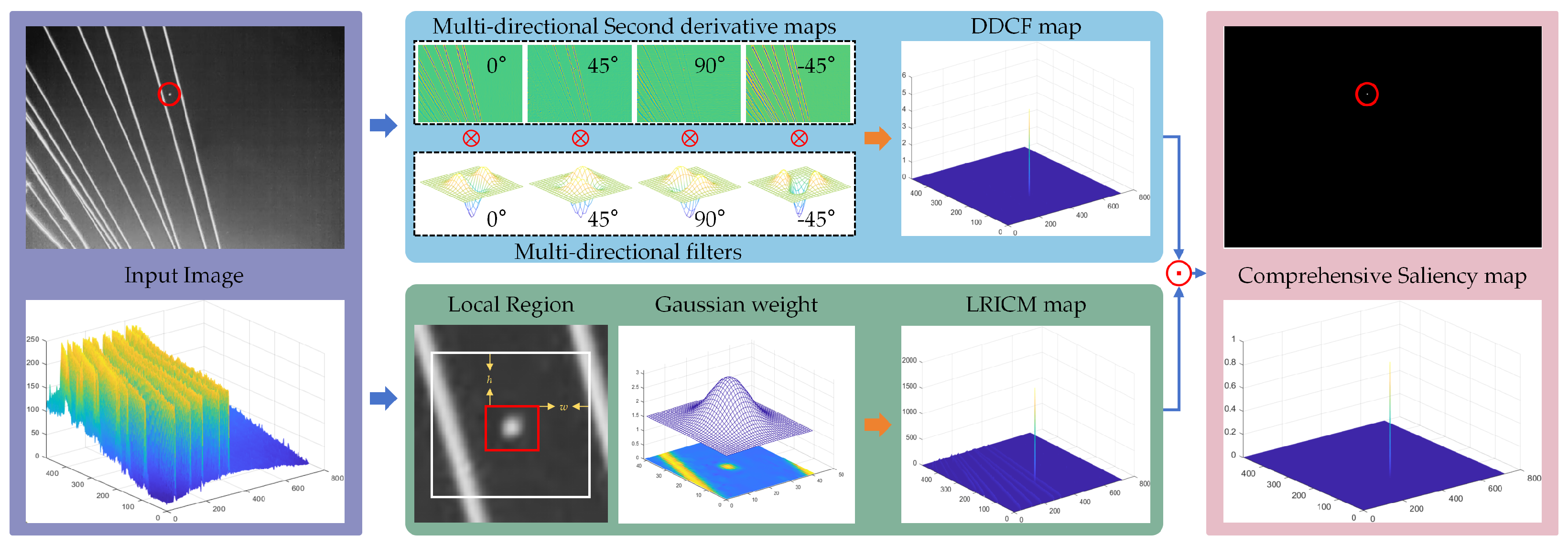
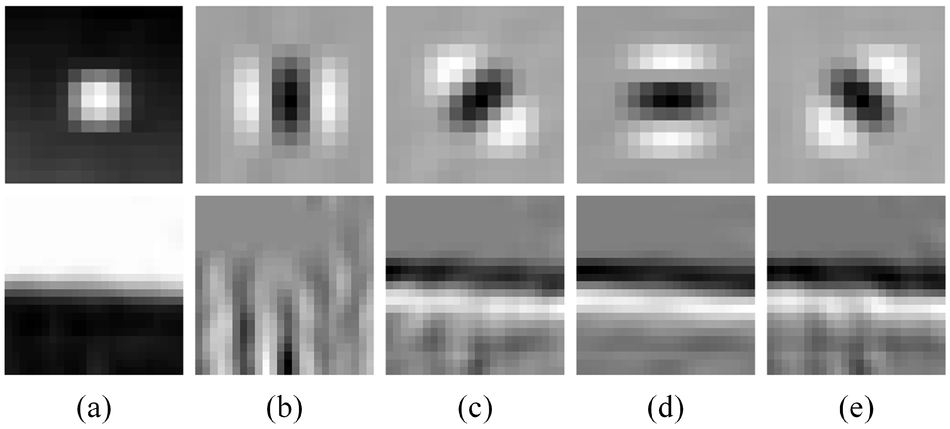
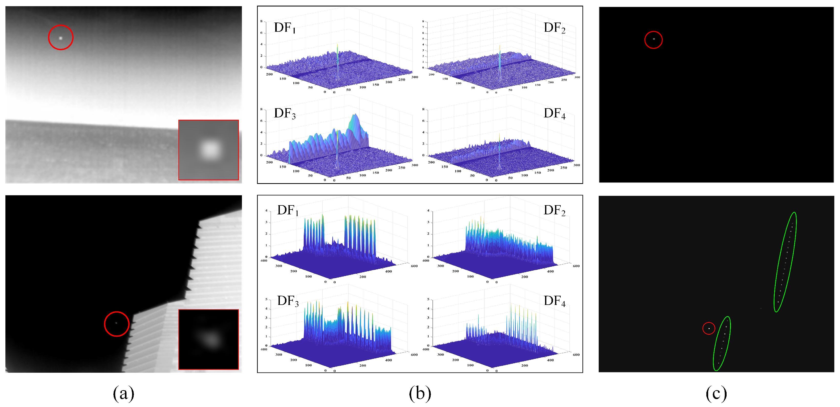
• A novel directional derivative correlation filtering (DDCF) method is proposed by thoroughly analyzing the differences in second-order derivative variations between small targets and background clutter. This method constructs four filters to process the second-order derivative maps of the image in different directions (0°, 45°, 90°, and −45°), generating a gradient saliency map that effectively eliminates edge clutter while enhancing the target signal.
• A new local relative intensity contrast measure (LRICM) method is introduced to improve the robustness of infrared small target detection. The LRICM method exploits the high contrast between small targets and their surroundings, addressing the limitations of DDCF in suppressing structural clutter such as corner interference.
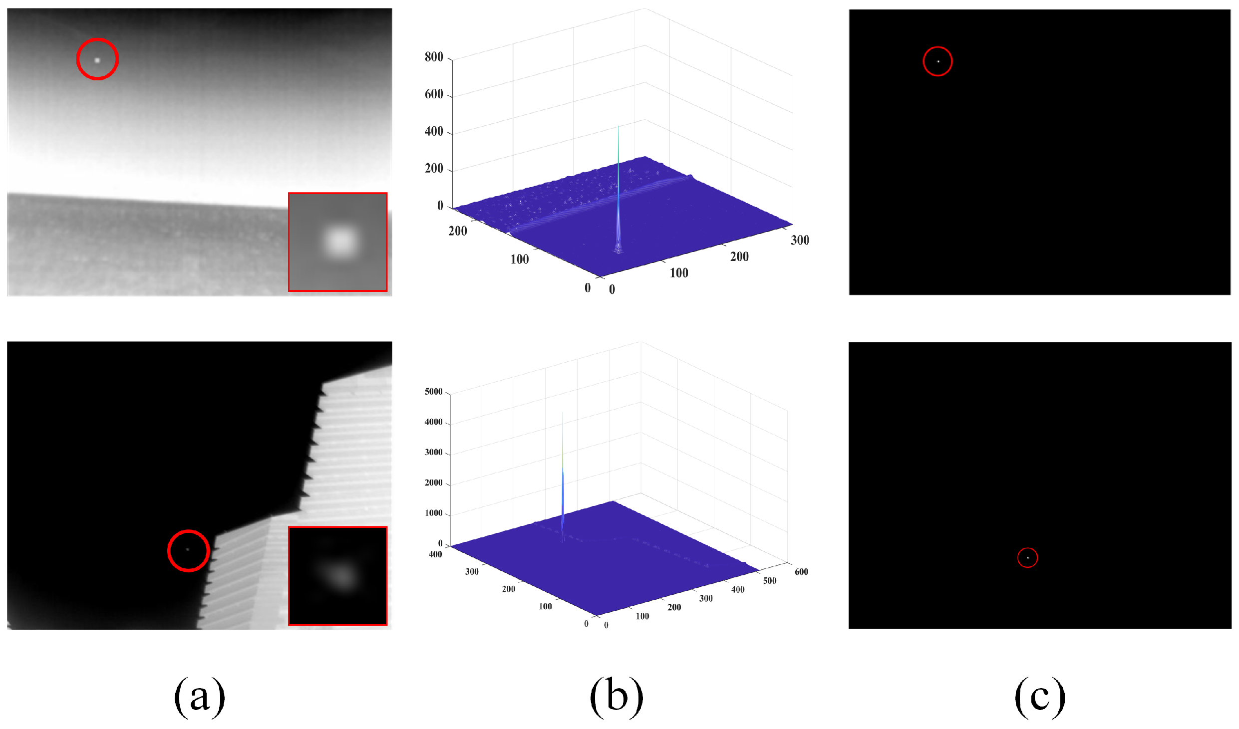
• An effective small target detection scheme is proposed by fusing the response maps of DDCF and LRICM for mutual compensation. The fused map ensures that the target intensity is fully enhanced while significantly suppressing background clutter, including edges and corners.

The remainder of the article is structured as follows. Section 2 provides a detailed description of the proposed small target detection scheme, including the DDCF and LRICM methods. Section 3 presents comparative experiments to validate the effectiveness of the proposed approach. Finally, Section 4 summarizes the main achievements obtained in this study.

2. Methodology

Figure 1 shows the framework of the proposed method, which integrates DDCF and LRICM. First, multi-directional second-order derivative maps of the input infrared image are constructed using the facet model. The DDCF map is then created based on the distinct gradient characteristics of small targets. Concurrently, the LRICM map is constructed by utilizing the center–surround contrast property of small targets. The final comprehensive saliency map is obtained by fusing the DDCF and LRICM maps. An adaptive threshold algorithm is then applied to locate the target.

2.1. Directional Derivative Computation Based on Facet Model

In contrast to gradient-based techniques [36], which calculate the gradient using two adjacent points, the facet model [37,38] is utilized to determine the directional derivative. This model represents the gray values within the neighborhood of each pixel using a binary cubic polynomial function. The pixel intensity function for a given neighborhood within the facet model can be formulated as

$$f(r,c)=\sum _{i=1}^{10}{K}_i\times P_i\left(r,c\right)$$

(1)

where $P_i(r,c)$ is composed of ten 2-D discrete orthogonal Chebyshev polynomials as

$$P_i\left(r,c\right)\in \left\{\begin{array}{c}1,r,c,r^2-c,rc,c^2-2,r^3-{\displaystyle \frac{17}{5}}r,\hfill \\ \left(r^2-2\right)c,r\left(c^2-2\right),c^3-{\displaystyle \frac{17}{5}}c\hfill \end{array}\right\}$$

(2)

where $[r,c]\in \{-2,-1,0,1,2\}$ represent the pixel position for a $5\times 5$ neighborhood. $K_i$ is the coefficient of polynomials that can be calculated by the least squares fitting method and defined as

$$K_i={\displaystyle \frac{{\sum }_r{\sum }_c{P}_i\left(r,c\right)f\left(r,c\right)}{{\sum }_r{\sum }_c{P}_i^2\left(r,c\right)}}$$

(3)

When computing the derivatives, $f(r,c)$ is derived from the original image, making it known. As a result, Equation (3) simplifies to $K_i=f(r,c)\otimes W_i$, where ⊗ denotes the correlation operator. The coefficient $W_i$ is defined as

$$W_i={\displaystyle \frac{P_i\left(r,c\right)}{{\sum }_r{\sum }_c{P}_i^2\left(r,c\right)}}$$

(4)

By substituting Equation (2) into Equation (4), the expression for $W_i$ is obtained as $W_i=w_i/sum\left(w_i^2\right)$. Furthermore, the relationships $W_3=W_2^T$, $W_6=W_4^T$, $W_9=W_8^T$, and $W_{10}=W_7^T$ hold, where $w_i$ are given by

$$\begin{array}{cc}{w}_1=\left[\begin{array}{ccccc}\hfill 1& 1& 1& 1& 1\\ \hfill 1& 1& 1& 1& 1\\ \hfill 1& 1& 1& 1& 1\\ \hfill 1& 1& 1& 1& 1\\ \hfill 1& 1& 1& 1& 1\end{array}\right]& w_2=\left[\begin{array}{ccccc}\hfill -2& -2& -2& -2& -2\\ \hfill -1& -1& -1& -1& -1\\ \hfill 0& 0& 0& 0& 0\\ \hfill 1& 1& 1& 1& 1\\ \hfill 2& 2& 2& 2& 2\end{array}\right]\end{array}$$

(5)

$$\begin{array}{cc}\begin{array}{cc}\hfill & w_4=\left[\begin{array}{ccccc}\hfill 2& 2& 2& 2& 2\\ \hfill -1& -1& -1& -1& -1\\ \hfill -2& -2& -2& -2& -2\\ \hfill -1& -1& -1& -1& -1\\ \hfill 2& 2& 2& 2& 2\end{array}\right]\hfill \\ \hfill & w_7=\left[\begin{array}{ccccc}\hfill -1& -1& -1& -1& -1\\ \hfill 2& 2& 2& 2& 2\\ \hfill 0& 0& 0& 0& 0\\ \hfill -2& -2& -2& -2& -2\\ \hfill 1& 1& 1& 1& 1\end{array}\right]\hfill \end{array}& \begin{array}{cc}\hfill & w_5=\left[\begin{array}{ccccc}\hfill 4& 2& 0& -2& -4\\ \hfill 2& 1& 0& -1& -2\\ \hfill 0& 0& 0& 0& 0\\ \hfill -2& -1& 0& 1& 2\\ \hfill -4& -2& 0& 2& 4\end{array}\right]\hfill \\ \hfill & w_8=\left[\begin{array}{ccccc}\hfill -4& -2& 0& 2& 4\\ \hfill 2& 1& 0& -1& -2\\ \hfill 4& 2& 0& -2& -4\\ \hfill 2& 1& 0& -1& -2\\ \hfill -4& -2& 0& 2& 2\end{array}\right]\hfill \end{array}\end{array}$$

(6)

Furthermore, the first-order and second-order derivatives [37] of $f(r,c)$ in any direction $\alpha$ can be computed as follows:

$$\begin{array}{cc}\hfill f_{\alpha }^{\prime }& ={\displaystyle \frac{\partial f}{\partial r}}sin\alpha +{\displaystyle \frac{\partial f}{\partial c}}cos\alpha \hfill \\ \hfill f_{\alpha }^{″}& ={\displaystyle \frac{{\partial }^{2}f}{\partial r^2}}{sin}^2\alpha +{\displaystyle \frac{{\partial }^{2}f}{\partial c^2}}{cos}^2\alpha +2{\displaystyle \frac{{\partial }^{2}f}{\partial r\partial c}}sin\alpha cos\alpha \hfill \end{array}$$

(7)

Finally, the partial derivatives of $f(r,c)$ at the center position of the neighborhood are calculated according to Equation (1) as follows:

$$\begin{array}{cc}\hfill {\left.{\displaystyle \frac{\partial f}{\partial r}}\right|}_{\left(0,0\right)}& =K_2-{\displaystyle \frac{17}{5}}{K}_7-2K_9\hfill \\ \hfill {\left.{\displaystyle \frac{\partial f}{\partial c}}\right|}_{\left(0,0\right)}& =K_3-{\displaystyle \frac{17}{5}}{K}_{10}-2K_8\hfill \\ \hfill {\left.{\displaystyle \frac{{\partial }^{2}f}{\partial r^2}}\right|}_{\left(0,0\right)}& =2K_4,{\left.{\displaystyle \frac{{\partial }^{2}f}{\partial c^2}}\right|}_{\left(0,0\right)}=2K_6,{\left.{\displaystyle \frac{{\partial }^{2}f}{\partial r\partial c}}\right|}_{\left(0,0\right)}=K_5\hfill \end{array}$$

(8)

By assigning different values to $\alpha$, the first-order and second-order derivatives of an infrared image in any given direction can be calculated using Equations (7) and (8).

2.2. Directional Derivative Correlation Filtering

Edge clutter has long been a major challenge in infrared small target detection, as it is challenging to remove using basic contrast-based methods. Recognizing the unique characteristics of small targets in directional derivatives, this paper introduces a detection algorithm that leverages second-order derivative maps of infrared images to effectively suppress strong edge clutter.

Figure 2 demonstrates the second-order derivatives of both the target and edge clutter in four directions (0°, 45°, 90°, and −45°). When detecting targets at long distances, factors such as energy attenuation and optical defocus in thermal imaging systems cause the target to appear as a circular bright spot, which aligns with the point spread function [27,39]. As a result, the second-order derivative of small targets exhibits a unique shape and amplitude that clearly distinguishes them from the background edge clutter, as shown in Figure 2. Regarding shape variation, the second-order derivatives of the target in each direction resemble the negative value of the DoG filters. In contrast, the second-order derivative of edge clutter changes smoothly in the 0° direction, with its amplitude concentrated around zero. Furthermore, as illustrated in Figure 2, the amplitude of the second-order derivatives for the target in all four directions is comparable and consistently higher than that of the background clutter.

Based on the above observations, four filters are designed to process the second-order derivatives of the infrared image in different directions, aiming to enhance the target. In this approach, the filter for a given direction $\alpha$ is defined as

$$\begin{array}{cc}\hfill F\left(x,y,\alpha \right)& ={\displaystyle \frac{1}{2\pi {\sigma }^4}}\times exp\left(-{\displaystyle \frac{x^2+y^2}{2{\sigma }^2}}\right)\times \left({\displaystyle \frac{{\left(xcos\alpha +ysin\alpha \right)}^2-1}{{\sigma }^2}}\right)\hfill \end{array}$$

(9)

where $\sigma$ represents the scale factor, which controls the amplitude and scale of the filter. The filter function F is derived from the derivative of a 2-D Gaussian function, ensuring that it mimics the change pattern of the second-order derivative of small targets in each direction. Additionally, the designed filter is normalized as $F=F/sum\left(F^2\right)$.

After the filter design is completed, a correlation operation is performed between the filters in different directions and the corresponding second-order derivatives of the infrared image. The multi-directional derivative correlation filtering in this method is expressed as

$$\begin{array}{cc}\hfill & {DF}_1\left(x,y\right)=f_{0°}^{″}\left(x,y\right)\otimes F\left(x,y,0°\right)\hfill \\ \hfill & {DF}_2\left(x,y\right)=f_{45°}^{″}\left(x,y\right)\otimes F\left(x,y,45°\right)\hfill \\ \hfill & {DF}_3\left(x,y\right)=f_{90°}^{″}\left(x,y\right)\otimes F\left(x,y,90°\right)\hfill \\ \hfill & {DF}_4\left(x,y\right)=f_{-45°}^{″}\left(x,y\right)\otimes F\left(x,y,-45°\right)\hfill \\ \hfill & {DF}_1\left({DF}_1<0\right)=0,{DF}_2\left({DF}_2<0\right)=0\hfill \\ \hfill & {DF}_3\left({DF}_3<0\right)=0,{DF}_4\left({DF}_4<0\right)=0\hfill \end{array}$$

(10)

where ⊗ represents the correlation operator. Any negative values in the response map are set to zero to suppress the background clutter. The filtering results in different directions are shown in Figure 3b. In this case, the edge clutter produces a significant response in just one direction, whereas the target exhibits large amplitudes across all four directional response maps. To differentiate the target from the background, the response maps from the four directions are fused as follows:

$$\mathrm{DDCF}\left(x,y\right)={DF}_1\left(x,y\right)·{DF}_2\left(x,y\right)·{DF}_3\left(x,y\right)·{DF}_4\left(x,y\right)$$

(11)

The value of $\sigma$ in Equation (9) is determined by the size of the target. In this study, it is assumed that the small target is an equilateral rectangle with dimensions $l\times l$. Considering that the neighborhood size in the facet model is $l_r\times l_c$ (with $l_r=l_c=5$), the size of the second-order directional derivative in the target area can be approximated as $d_{sz}=l+l_r-1$. Based on this, the value of $\sigma$ is set according to the following relationship:

$$\sigma ={\displaystyle \frac{d_{sz}-1}{2\times k}}={\displaystyle \frac{l+l_r-2}{2\times k}}$$

(12)

The value of k is a coefficient that controls the shape of the proposed filter. Figure 4 illustrates the side view of the filter in the $\alpha =0°$ direction for various parameter settings. In this study, the coefficient k is set to $k=4$.

The final fused DDCF map is presented in Figure 3c. After filtering, most of the strong edge clutter in the raw image is effectively removed, and the target’s intensity is substantially enhanced. While some background clutter remains in individual directional response maps, the fusion process helps cancel out the intensities of non-target points, leaving only the target visible. However, the DDCF method shows some sensitivity to specific corner clutter. In addition, we calculated the signal-to-noise ratio gain (SCRG) and background suppression factor (BSF) metrics [40] of the DDCF maps. The SCRG values are $0.2561\times {10}^5$ and $0.0216\times {10}^5$, and the BSF values are $0.1496\times {10}^5$ and $0.1912\times {10}^5$, respectively. These results demonstrate that the DDCF method is more effective in suppressing edge clutter.

2.3. Local Relative Intensity Contrast Measure

By utilizing the distinctive second-order derivative properties of small targets, the DDCF map is calculated to enhance the target while suppressing edge clutter. Experimental results reveal that the DDCF method is sensitive to certain corner clutter. To address this limitation, a local relative intensity contrast measure (LRICM) is introduced, leveraging the fact that small targets generally exhibit higher intensity than their surrounding regions. The method begins by defining the center region and its local background, as illustrated in Figure 1, where w and h represent the width and height of the center area, highlighted by the red rectangle. The region between the white and red rectangles represents the local background. Unlike conventional local contrast measures [16], this approach uses the minimum intensity in the local background as a reference and introduces a novel relative contrast measure defined as

$$RC={\displaystyle \frac{m_t-L_b}{m_b-L_b}}$$

(13)

where $m_t$ and $m_b$ represent the mean gray values of the center region and the local background region, respectively. $L_b$ is the minimum gray value of the local background region. To evaluate the effectiveness of target enhancement and background suppression, the proposed relative contrast measure is compared to the traditional contrast measure ($C={\displaystyle \frac{m_t}{m_b}}$) using the following ratio:

$$r={\displaystyle \frac{RC}{C}}={\displaystyle \frac{m_t-L_b}{m_b-L_b}}\times {\displaystyle \frac{m_b}{m_t}}$$

(14)

Moreover, Equation (14) can be decomposed in the form:

$$r=1+r_1\times r_2,\mathrm{and}{r}_1=1-{\displaystyle \frac{m_b}{m_t}},r_2={\displaystyle \frac{L_b}{m_b-L_n}}$$

(15)

Based on Equation (15), the following conclusions can be drawn:

• r is a non-negative value, with $r_2>0$.
• When the center region represents the target, its intensity $m_t$ is greater than that of the surrounding region $m_b$, so $r_1>0$ and $r>1$. This implies that $RC>C$, indicating that the relative contrast $RC$ has stronger target enhancement capabilities than the traditional contrast C.
• When the center region represents the local background, its intensity $m_t$ is typically less than or equal to that of the surrounding region $m_b$. If $m_t=m_b$, then $r=1$ and $RC=C$. If $m_t<m_b$, then $r_1<0$, which results in $0<r<1$. In this case, $0<RC<C<1$, demonstrating that the relative contrast $RC$ provides better background suppression than the traditional contrast C.

Based on the analysis above, it is inferred that the proposed relative contrast method outperforms traditional contrast in both target enhancement and background suppression. To quantify the overall effectiveness across the local region, the enhancement factor (EF) is defined as

$$EF={\displaystyle \frac{{\left(m_t-L_b\right)}^2}{{\sum }_{i,j\in {\mathrm{\Omega }}_b}\left(g\left(i,j,{\sigma }_b\right)\times {\left(I_b\left(i,j\right)-L_b\right)}^2\right)+{\epsilon }_0}}$$

(16)

where ${\mathrm{\Omega }}_b$ represents the set of pixel coordinates in the local background region, and $I_b(i,j)$ denotes the gray value at the corresponding coordinate position. To avoid division by zero, ${\epsilon }_0$ is introduced as a positive constant. As pixels farther from the central region have a decreasing influence on the enhancement, a Gaussian function is applied to weight the pixels in the local background. This weighting decreases the impact of pixels located farther away from the central region, as shown in Figure 1. The Gaussian function g is defined as

$$g\left(i,j,{\sigma }_b\right)={\displaystyle \frac{1}{2\pi {\sigma }_b^2}}exp\left(-{\displaystyle \frac{i^2+j^2}{2{\sigma }_b^2}}\right),i,j\in {\mathrm{\Omega }}_b$$

(17)

where ${\sigma }_b$ is the scale factor, and in this study, it is set to ${\sigma }_b=l/2$, with l representing the size of the central region. The Gaussian function is normalized to ensure that the sum of its values equals 1, i.e., $sum\left(g\right)=1$. To enhance the target further, the local relative intensity contrast measure (LRICM) for a target size of $l\times l$ can be defined as:

$$\mathrm{LRIC}{\mathrm{M}}^l=\left|m_t-m_b\right|\times EF, \mathrm{and}\mathrm{LRIC}{\mathrm{M}}^l\left(m_t-m_b<0\right)=0$$

(18)

To address the challenges originating from unknown target sizes, a multi-scale approach is utilized for small target detection. In this approach, LRICM is defined as

$$\mathrm{LRICM}=\underset{l\in {\mathrm{\Omega }}_l}{max}\left(\mathrm{LRIC}{\mathrm{M}}^l\right)$$

(19)

where ${\mathrm{\Omega }}_l$ represents the target scale space, which can be adjusted based on the specific conditions. The LRICM indicates the prominence of targets relative to the surrounding background, with higher values signaling more distinct targets. By scanning the entire infrared image, the LRICM map is generated. As shown in Figure 5b, the LRICM map of the raw images illustrates that much of the background clutter, including angular clutter, has been suppressed, thereby improving the visibility of the targets. Furthermore, we calculated the SCRG and BSF metrics for the LRICM maps and the CR maps. For Scene 1, the SCRG and BSF values of the LRICM maps are $0.0032\times {10}^5$ and $0.1200\times {10}^5$, respectively, while those of the CR maps are $38.5624\times {10}^5$ and $0.1685\times {10}^5$. For Scene 2, the SCRG and BSF values of the LRICM maps are $0.2444\times {10}^5$ and $0.2516\times {10}^5$, and those of the CR maps are $8.1529\times {10}^5$ and $0.3556\times {10}^5$. These results indicate that LRICM has stronger corner clutter suppression capability, and the fused CR method, derived from DDCF and LRICM, achieves the best detection performance under both edge and corner clutter backgrounds.

2.4. Target Detection Using DDCF and LRICM

The preceding analysis demonstrates that the DDCF and LRICM maps exhibit distinct and complementary advantages in background suppression and target enhancement. Ideally, true targets produce strong responses in both maps, while background clutter yields low values. As a result, multiplicative fusion effectively amplifies the contrast between targets and the background, thereby enhancing detection performance. Based on this rationale, we employ a pixel-wise multiplicative operation to fuse the DDCF and LRICM maps into a comprehensive response (CR) map of the original infrared image, which is expressed as

$$\mathrm{CR}\left(x,y\right)=\mathrm{DDCF}\left(x,y\right)\times \mathrm{LRICM}\left(x,y\right)$$

(20)

Before fusion, it is essential to normalize the DDCF map and LRICM map to ensure consistent magnitude levels. Figure 5c illustrates the CR map of the raw images, where edge and corner clutter have been significantly reduced, facilitating the detection of targets.

After computing the CR map, targets can be extracted by applying an appropriate threshold. In this study, the segmentation threshold is defined as

$$\mathrm{Th}={\mu }_{\mathrm{CR}}+\lambda \times {\sigma }_{\mathrm{CR}}$$

(21)

where ${\mu }_{\mathrm{CR}}$ and ${\sigma }_{\mathrm{CR}}$ represent the mean and standard deviation of the CR map, respectively. $\lambda$ is an empirical constant that adjusts according to changes in the IR scene. The range of $\lambda$ will be further discussed in the ablation experiments. Once the segmentation threshold is established, pixels with values exceeding the threshold are classified as targets, while the remaining pixels are considered part of the background. Algorithm 1 provides a detailed description of the computation process for generating the CR map.

Algorithm 1 Infrared Small Target Detection Using DDCF and LRICM.

Input: An infrared image, $\alpha =0°$, $45°$, $90°$, and $-45°$ Output: The segmented target image 1: Calculate the second-order directional derivatives of infrared image based on the facet model with Equations (1)–(8). 2: Calculate the filters in four directions (0°, 45°, 90°, and −45°) according to Equation (9). 3: Acquire the directional derivative correlation filtering (DDCF) map to suppress the edge clutter according to Equations (10) and (11). 4: Obtain the local relative intensity contrast measure (LRICM) map to eliminate the corner clutter with Equations (13)–(19). 5: Integrate the DDCF map and LRICM map to obtain the comprehensive response (CR) map according to Equation (20). 6: Extract the real target from the CR map with the segmented target image.

3. Experiments

This section presents several comparative experiments to evaluate the small target detection performance of the proposed algorithm. First, the experimental setup is described, including details on the dataset, baseline methods, and evaluation metrics. Next, a series of tests are conducted on the dataset to determine the optimal filter parameter $\sigma$ in Equation (9). Finally, the proposed algorithm is compared with baseline methods through both qualitative and quantitative experiments. All simulations and experiments are executed on a PC equipped with 16.0 GB of memory and a 2.10-GHz Intel i7 processor, with the code implemented in MATLAB 2024a.

3.1. Experimental Setup

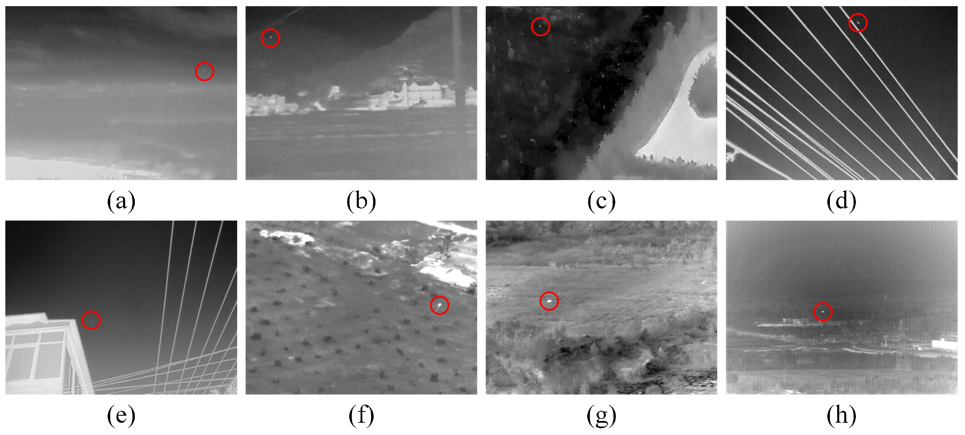
3.1.1. Dataset

For the experiments conducted in this section, eight distinct test sequences, each representing different scenarios, are utilized. These sequences are labeled as Seq_1-Seq_3 [41], Seq_4-Seq_5 [42], and Seq_6-Seq_8 [43]. Representative images from these sequences, with targets marked by red circles, are shown in Figure 6. The scenarios and corresponding images are as follows:

Figure 6a: A small target in a scene with a cloudy sky and intense interference from a lake.

Figure 6b: A target situated in a mountainous environment with substantial building interference.

Figure 6c: A pedestrian target hidden in a bushy area.

Figure 6d: A small craft flying through the sky, with complex wires highlighted in the scene.

Figure 6e: A small airplane flying in front of a bright building and wires.

Figure 6f,g: A downward-facing view of a small drone in flight, surrounded by high-contrast rocks and bushes.

Figure 6h: A small fixed-wing aircraft flying in a mountainous setting, with numerous buildings providing high contrast.

The specific details of each sequence are provided in

Table 1. Detailed information on test datasets.

Sequences	Frames	Resolutions	Target Size and Shape	Background Description
Seq_1	100	640 × 480	•  $5\times 5$∼$9\times 9$	•  Heavy clouds
			•  Triangle shaped	•  High-intensity lake interference
Seq_2	100	320 × 240	•  $5\times 5$∼$9\times 9$	•  Intense building interference
			•  From point to triangle shape	•  Heavy edges and corners
Seq_3	100	640 × 480	•  $9\times 9$∼$15\times 15$	•  High-intensity bushes
			•  Variable shape	•  Shrub clutter of different scales
Seq_4	250	720 × 480	•  $5\times 5$∼$9\times 9$	•  High-brightness wires
			•  Point shape	•  Heavy edges
Seq_5	275	720 × 480	•  $3\times 3$∼$7\times 7$	•  Intense building interference
			•  Point shape	•  High-brightness wires
Seq_6	200	256 × 256	•  $3\times 3$∼$7\times 7$	•  High-intensity stones
			•  Ellipse shape	•  Dense Forest interference
Seq_7	280	256 × 256	•  $5\times 5$∼$9\times 9$	•  Shrub clutter
			•  Circular shape	•  Scattered stones
Seq_8	1200	256 × 256	•  $3\times 3$∼$7\times 7$	•  Intense building interference
			•  Point shape	•  Thick forest interference

.

3.1.2. Baseline Methods

Seven state-of-the-art infrared small target detection algorithms are employed as baseline methods in this study. These include PSTNN [44], ADDGD [45], MPCM [19], ADMD [14], FKRW [22], ELUM [4], and HBMLCM [21]. The PSTNN method is based on tensor operations. The ADDGD, MPCM, ADMD, FKRW, and HBMLCM methods are all driven by the HSV color model. ELUM is a technique that utilizes a local component uncertainty measure along with consistency evaluation.

3.1.3. Evaluation Metrics

The performance of single-frame infrared small target detection algorithms is usually assessed using the signal-to-noise ratio gain (SCRG) and background suppression factor (BSF) [40]. These metrics are defined as

$$\mathrm{BSF}={\displaystyle \frac{{\sigma }_{\mathrm{in}}}{{\sigma }_{\mathrm{out}}}},\mathrm{SCRG}={\displaystyle \frac{\mathrm{SC}{\mathrm{R}}_{\mathrm{out}}}{\mathrm{SC}{\mathrm{R}}_{\mathrm{in}}}},\mathrm{SCR}={\displaystyle \frac{\left|{\mu }_t-{\mu }_b\right|}{{\sigma }_b}}$$

(22)

where ${\sigma }_{\mathrm{in}}$ and ${\sigma }_{\mathrm{out}}$ represent the standard deviations of the input image and the response map, respectively. ${\mu }_t$ is the mean value of the target, while ${\mu }_b$ and ${\sigma }_b$ correspond to the mean and standard deviation of the image excluding the target.

Furthermore, the receiver operating characteristic (ROC) curve is employed to assess the detection performance of various algorithms across an image sequence. The ROC curve plots the false positive rate (FPR) on the x-axis against the true positive rate (TPR) on the y-axis, varying the segmentation threshold. The definitions of TPR and FPR [4,38] are

$$\begin{array}{cc}\hfill & \mathrm{TPR}={\displaystyle \frac{\mathrm{number}\mathrm{of}\mathrm{true}\mathrm{target}\mathrm{detection}}{\mathrm{number}\mathrm{of}\mathrm{actual}\mathrm{targets}}}\hfill \\ \hfill & \mathrm{FPR}={\displaystyle \frac{\mathrm{number}\mathrm{of}\mathrm{false}\mathrm{pixels}\mathrm{detection}}{\mathrm{number}\mathrm{of}\mathrm{total}\mathrm{pixels}\mathrm{in}\mathrm{images}}}\hfill \end{array}$$

(23)

The area under the ROC curve (AUC) serves as an indicator of the target detection performance. A larger AUC value, along with a curve closer to the upper left corner, signifies superior detection performance.

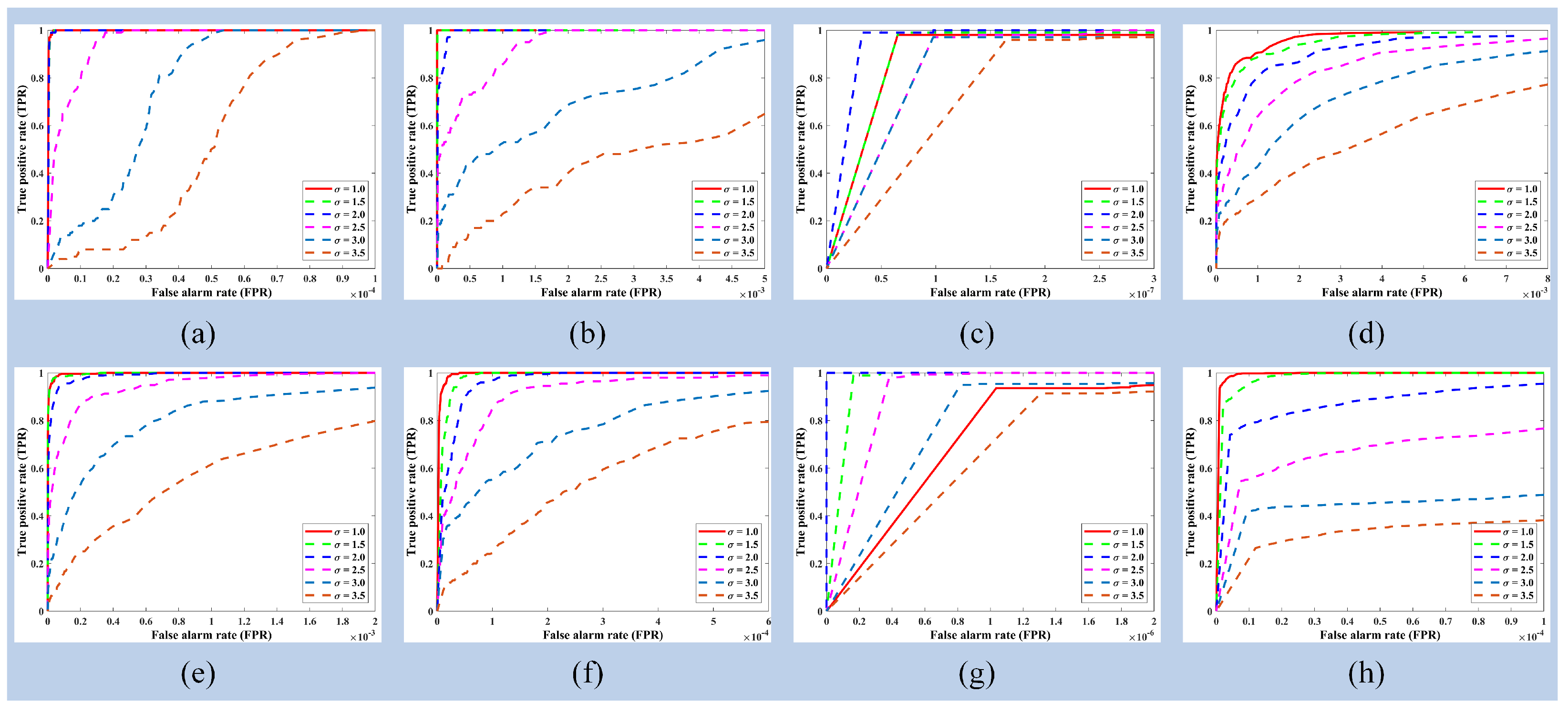
3.2. Parameter Configurations

The DDCF method relies on a key parameter, $\sigma$, which must be optimized for effective background suppression and target enhancement. To determine the optimal value of $\sigma$ for each sequence, SCRG and BSF metrics are employed on the test dataset. Equation (12) indicates that $\sigma$ is related to the target size. Based on the target sizes listed in Table 1, different values of $\sigma$ are tested and the corresponding SCRG and BSF are calculated for each. The results are summarized in

Table 2. SCRG and BSF values of the DDCF map with different parameter $\sigma$ configurations for the test dataset.

Metrics	Parameter	Sq_1	Sq_2	Sq_3	Sq_4	Sq_5	Sq_6	Sq_7	Sq_8
SCRG	$\sigma =1.0$	1118.58	257.756	5743.40	53.8909	541.623	378.040	932.966	503.552
	$\sigma =1.5$	634.270	158.668	8370.83	50.4575	436.577	273.071	1102.96	332.623
	$\sigma =2.0$	381.609	77.0201	9870.55	39.1242	266.048	149.595	1006.53	184.651
	$\sigma =2.5$	180.754	32.0840	8600.44	26.6670	138.703	64.8665	679.658	91.0055
	$\sigma =3.0$	78.2715	12.0105	6294.97	16.5672	67.0746	28.9064	386.735	42.6790
	$\sigma =3.5$	38.6712	4.19143	4277.85	9.60601	31.3070	17.0965	194.779	19.5860
BSF	$\sigma =1.0$	17,951.4	7106.61	12,733.8	8896.81	17,462.9	3495.58	6789.94	5783.71
	$\sigma =1.5$	15,568.2	5666.59	11,984.6	8223.98	14,836.0	3149.57	6449.29	5187.79
	$\sigma =2.0$	12,907.6	4102.07	11,286.9	8130.35	11,140.2	2825.26	5955.27	4493.41
	$\sigma =2.5$	10,480.9	2845.80	10,569.4	7291.23	8489.69	2390.03	5339.90	3603.10
	$\sigma =3.0$	10,309.4	2279.07	9698.69	5720.58	7294.63	1731.09	4735.32	3048.38
	$\sigma =3.5$	9942.20	2273.83	8807.85	6002.19	6974.20	1498.81	4029.35	2636.22

. When $\sigma =1$, the BSF values for all test data are relatively high, indicating effective background suppression. However, increasing $\sigma$ beyond a certain point leads to a significant decrease in SCRG and BSF due to the introduction of excessive clutter interference. Specifically, for Seq_3, the DDCF method shows optimal target enhancement when $\sigma =2.0$, which aligns with the target size in Seq_3 as indicated by Equation (12). Therefore, the optimal parameter value for each sequence can be set in accordance with this relationship, optimizing the target enhancement capabilities of the DDCF method. Additionally, ROC curves for different parameter values show a pattern similar to SCRG and BSF, as depicted in Figure 7. Based on these findings, the optimal values of $\sigma$ for sequences Seq_1 through Seq_8 are set to 1, 1, 2, 1, 1, 1, 1.5, and 1, respectively, for the subsequent experiments.

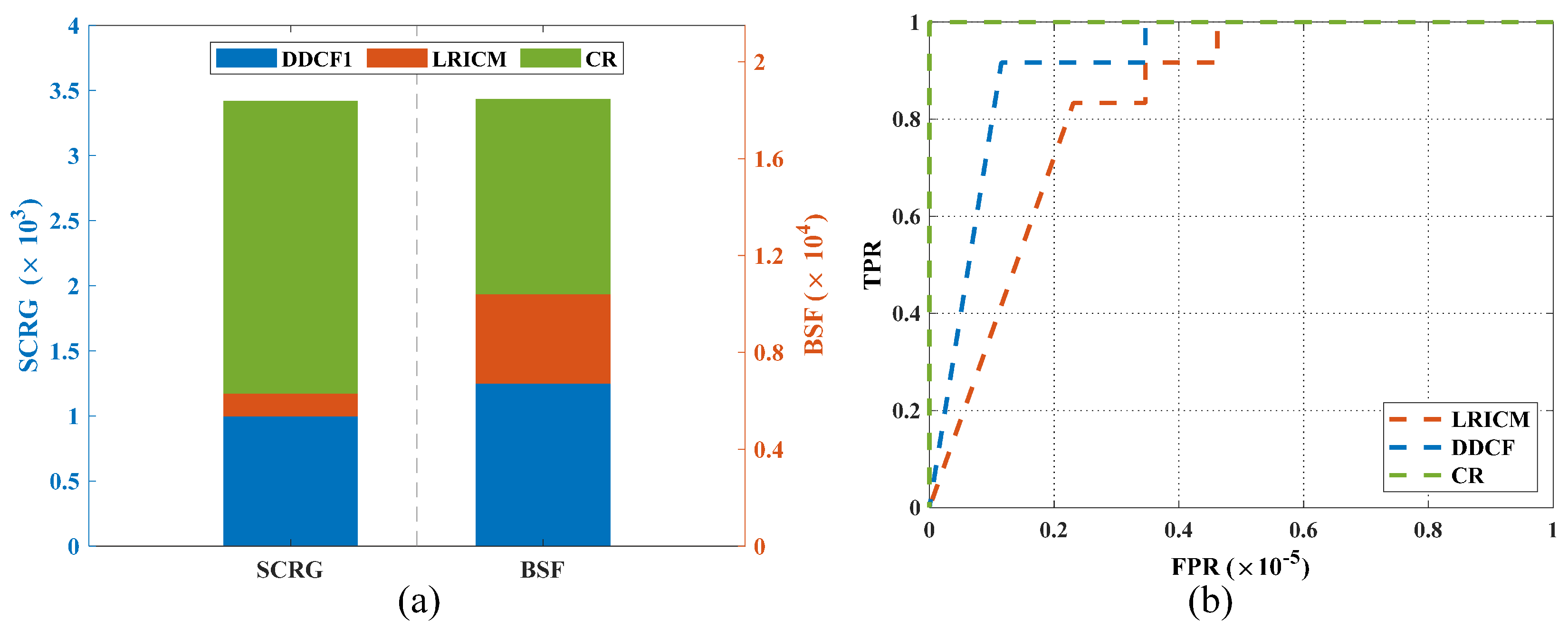
3.3. Ablation Experiments

Ablation experiments were conducted on the SIRST dataset [46] to assess the individual contributions of DDCF and LRICM to the proposed algorithm. Twelve representative images are shown in Figure 8, along with their corresponding DDCF maps, LRICM maps, and CR maps. These images present complex backgrounds, including buildings, clouds, and forests, as well as clutter such as edges, PNHB, and corners.

In Figure 8(a1,a3,e3,e4), the presence of significant edge clutter leads to considerable residual interference in the corresponding LRICM maps, as seen in Figure 8(c1,c3,g3,g4). However, when the DDCF method is applied, this edge clutter is nearly fully suppressed, effectively addressing the limitations of the LRICM algorithm, as shown in Figure 8(b1,b3,f3,f4). In Figure 8(b2,e1,e2), sky backgrounds with cloud clutter and PNHB are depicted. As observed in Figure 8(c2,e1), LRICM successfully removes interference caused by dense cloud layers but struggles with fragmented clouds. In contrast, Figure 8(b2,f1) show that DDCF effectively suppresses cloud backgrounds. The fusion-based CR map also results in a higher SCR, making target extraction easier, as demonstrated in Figure 8(d2,h1).

In Figure 8(a4), dark circular spots emerge as the primary interference, presenting a notable challenge for the DDCF algorithm, as seen in Figure 8(b4). However, the LRICM method effectively removes these spots, as shown in Figure 8(c4). Moreover, the CR map combines the strengths of both methods, resulting in enhanced detection performance, as illustrated in Figure 8(d4). In Figure 8(a5), the corners of buildings and edges of walls significantly hinder detection, representing a major challenge in infrared small target detection. As seen in Figure 8(b5,c5), the DDCF algorithm effectively suppresses edge clutter but remains sensitive to corner clutter, while the LRICM method reduces corner clutter but still retains some edge interference. After merging the DDCF and LRICM maps in Figure 8(d5), both edge and corner clutter are eliminated, leaving only the target visible in the CR map.

In Figure 8(a6), bright shrubs present a substantial challenge for target detection, with both the DDCF and LRICM maps retaining some clutter that hinders accurate target localization. However, in the CR map, these interferences are further suppressed, making the target detection task easier. Figure 8(e5) contains minor edge clutter, which does not significantly affect the performance of the DDCF and LRICM algorithms, as shown in Figure 8(f5,g5,h5). In Figure 8(e6), the uneven brightness distribution of the mountainous terrain greatly interferes with the detection of infrared small targets. As seen in Figure 8(f6,g6,h6), although both the DDCF and LRICM maps still contain significant interference, much of it is eliminated in the CR map.

Additionally, the SCRG and BSF values for the DDCF, LRICM, and CR maps were calculated on the SIRST dataset, and the corresponding ROC curves were plotted, as shown in Figure 9. The results demonstrate that the CR method leverages the strengths of both the DDCF and LRICM algorithms, leading to superior detection performance compared to each method individually. This highlights the effectiveness of combining DDCF and LRICM.

In summary, the DDCF algorithm exhibits superior performance in managing edge clutter, while the LRICM method is particularly effective at suppressing dark spots and corner clutter. Together, these two methods complement one another, allowing the proposed algorithm to efficiently handle a wide variety of background clutter types.

Finally, we discuss the selection range of the parameter $\lambda$ in Equation (9) on the SIRST dataset. An optimal value of $\lambda$ should maximize the detection performance of the CR method. Based on this principle, we plot the curves of TPR and FPR under different values of $\lambda$, as shown in Figure 10. It can be observed that as $\lambda$ increases, both TPR and FPR gradually decrease. The FPR approaches zero and reaches a minimum value of 0.000338 when $\lambda =5$, indicating a low number of false alarms. Meanwhile, the TPR begins to decline significantly at $\lambda =25.7$, suggesting that some targets are missed at this point. To achieve a balanced and favorable detection performance, we set the range of $\lambda$ to $[5,25.7]$ in this study.

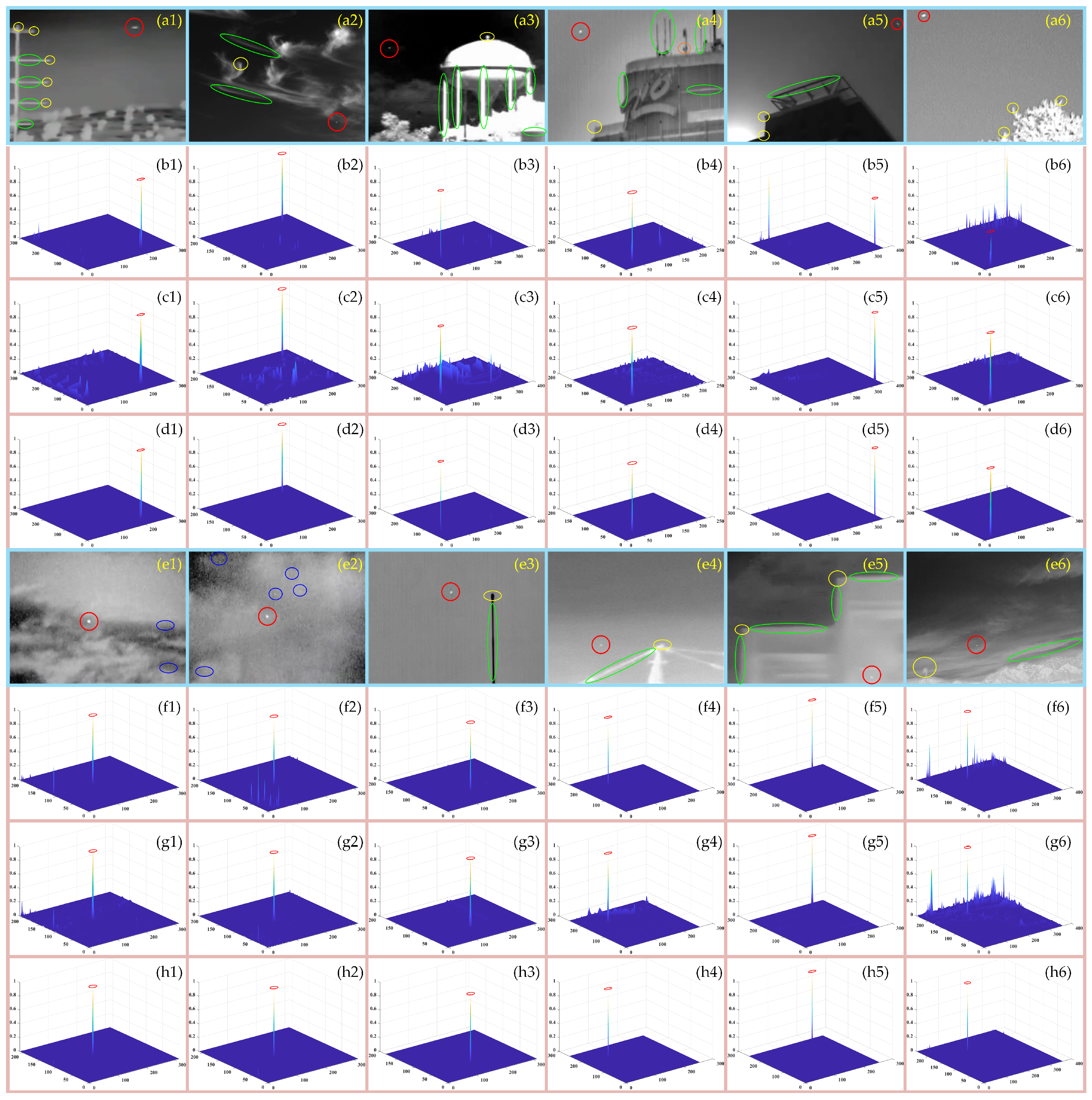
3.4. Visual Comparisons

Detection experiments were conducted on the eight infrared image sequences, and the results of our method and baseline methods for Figure 6 are presented in Figure 11. As shown in Figure 11a, the proposed method demonstrates superior target enhancement and clutter suppression across all eight images when compared to the baseline methods. Notably, after applying the proposed approach, background clutter is nearly completely removed from all images, leaving only the prominent targets, which can be easily extracted using an adaptive threshold segmentation technique.

As illustrated in Figure 11b, the PSTNN method is effective in suppressing most background clutter, including edges, but struggles with high-intensity corner clutter, as seen in Figure 6b,f. A comparison of Figure 11c,e shows that both ADDGD and ADMD rely on the average absolute gray difference between the target and its surroundings. However, ADMD performs better in dealing with strong edge clutter due to its incorporation of orientation information, as seen in Figure 6d,e.

Both MPCM and HBMLCM are contrast-based methods. The MPCM method enhances the central patch by calculating the difference with the eight surrounding patches and selecting the smallest difference as the enhancement factor, offering stronger edge suppression capabilities than HBMLCM, as demonstrated in Figure 11d,h. As shown in Figure 11g, the ELUM method effectively suppresses some fragmented background clutter but struggles with strong edge clutter.

In conclusion, the proposed method effectively leverages second-order directional derivatives and intensity features of infrared small targets to robustly suppress intense background clutter, including edges and corners, while effectively enhancing the targets. It demonstrates superior performance compared to baseline algorithms in visual assessments.

3.5. Quantitative Comparisons

The detection performance of the proposed method, along with the baseline methods, is further evaluated using SCRG, BSF, and ROC curves. The SCRG and BSF values for each method on Seq_1 to Seq_8 are presented in

Table 3. SCRG and BSF values of allaalgorithms.

Metrics	Parameter	Seq_1	Seq_2	Seq_3	Seq_4	Seq_5	Seq_6	Seq_7	Seq_8
SCRG	Ours	5327.23	2161.24	152,881	765.581	5317.51	4701.86	11,838.7	14,188.2
	PSTNN	118.056	25.4970	809.482	18.0156	183.449	33.7244	55.7637	31.8761
	ADDGD	187.299	21.9029	1237.00	4.66084	111.812	73.0348	125.696	130.914
	MPCM	116.611	20.4532	285.355	16.9110	225.730	47.2806	69.8973	67.2748
	ADMD	164.246	26.2851	332.135	17.4413	349.424	51.7063	92.8936	76.2349
	FKRW	385.183	175.569	281.145	92.2765	764.785	32.8007	38.8072	232.315
	ELUM	430.034	98.9511	88.0780	6.31599	115.720	66.0011	39.9629	125.680
	HBMLCM	73.3710	12.9106	748.422	2.36939	24.3549	58.7251	199.192	58.8405
BSF	Ours	20,522.0	8685.67	13,784.1	17,645.5	29,336.8	4002.49	7210.42	6836.73
	PSTNN	6178.88	1940.94	5295.24	4366.78	6842.73	1203.36	2259.84	2123.18
	ADDGD	10,379.0	2711.69	9082.53	3096.04	5965.53	2513.48	4564.98	4345.26
	MPCM	7243.25	1978.23	6975.03	2679.28	9089.19	1997.54	3731.93	3321.58
	ADMD	9490.52	2192.33	8047.79	4593.21	10,995.6	2252.68	4383.71	3545.21
	FKRW	9262.52	4999.54	7208.32	9311.87	12266.8	1540.51	3520.87	3252.49
	ELUM	12,721.3	5153.07	6497.50	1384.51	3030.48	2399.49	2986.55	5138.71
	HBMLCM	7029.30	1896.11	9162.27	1188.53	2035.65	2154.98	5025.96	2969.10

, with the highest values highlighted in bold and the second-highest values italicized and underlined. The results show that the proposed algorithm consistently achieves the highest SCRG and BSF values across all sequences, highlighting its effectiveness in addressing various complex background interferences.

PSTNN constructs a tensor structure using local image patches and extracts small targets based on low-rank and sparse decomposition. As shown in Table 3, it performs well in smooth background scenarios and is capable of suppressing a certain amount of edge clutter. For instance, in Seq_3 and Seq_4, PSTNN achieves higher SCRG values than most baseline methods. However, its detection performance is limited in scenarios with strong corner clutter interference, such as Seq_5. In sequences with significant edge clutter, such as Seq_4 and Seq_5, the FKRW method achieves higher SCRG and BSF values, but its performance in target enhancement and background suppression is still inadequate for Seq_6. On the other hand, the ADDGD method shows the lowest SCRG and BSF values in Seq_4 and Seq_5, yet it performs better in Seq_6, indicating its limitation in handling strong edge clutter but effective suppression of fragmented bright areas. Due to the lack of directional modeling, MPCM exhibits a significant performance decline in structurally complex or strongly edged backgrounds. For example, in Seq_4, both its SCRG and BSF values are lower than those of ADDGD and ADMD, which are also contrast-based methods. The ADMD method suppresses background interference by minimizing the directional mean difference. By incorporating directional information, it achieves stable performance across various scenarios (e.g., Seq_2, Seq_4, and Seq_5), outperforming other local contrast-based algorithms. However, in other sequences (such as Seq_7 and Seq_8), ADMD underperforms compared to other methods, indicating its limited adaptability to complex backgrounds. The HBMLCM method improves upon LCM but lacks directional information, resulting in subpar detection performance in Seq_2, Seq_4, and Seq_5. However, in Seq_7, where the background is relatively smooth and dim, HBMLCM achieves the second-best results for both target enhancement and background suppression. Although the ELUM method performs well in several sequences, it struggles with strong edge clutter, as seen in Seq_4 and Seq_5, demonstrating that such clutter remains a significant challenge even for advanced algorithms.

This study presents an algorithm that leverages the second-order directional derivative characteristics of infrared targets across four directions, effectively reducing edge and corner clutter. Furthermore, it enhances the saliency of targets by utilizing intensity contrast features in the grayscale domain. The integration of these two strategies leads to notable improvements in both target enhancement and background suppression.

The ROC curves for all algorithms are presented in Figure 12. The curves for the proposed method show a rapid rise across all eight sequences, indicating the effective elimination of most background clutter in the infrared images. Furthermore, the TPR in the ROC curves reaches or nears 1, signifying that nearly all targets are detected, highlighting the excellent performance in target enhancement.

In contrast, although other algorithms may perform well on some sequences, they struggle with others and fail to handle all complex scenarios. For instance, while the ROC curve of the ELUM method exceeds the performance of most algorithms on Seq_1, it performs poorly on other sequences. Similarly, in Seq_3, the PSTNN method’s TPR increases rapidly with a rising FPR, outperforming most algorithms, but on Seq_5 and Seq_7, the TPR rises more slowly, suggesting that significant interference remains in the processed response maps.

The quantitative comparison experiments demonstrate that the proposed algorithm demonstrates notable advantages in both accuracy and robustness across a variety of complex scenes.

3.6. Computational Efficiency

In this section, the computational complexity of the proposed algorithm is analyzed, and the average processing time of various algorithms is compared. The results are presented in

Table 4. Computational complexity and time consumption of different algorithms.

Methods		Ours	PSTNN	ADDGD	MPCM	ADMD	FKRW	ELUM	HBMLCM
Complexity		$O\left(MN{l}^2+MN{L}^2\right)$	$O\left(\begin{array}{c}{n}_1{n}_2{n}_{3}log\left(n_1{n}_2{n}_3\right)\hfill \\ +n_1{n}_2^2\left[(n_3+1)/2\right]\hfill \end{array}\right)$	$O\left(MN{L}^2\right)$	$O\left(MN{L}^2\right)$	$O\left(MN{L}^2\right)$	$O\left(MN{L}^3\right)$	$O\left(MN\right)$	$O\left(MN{L}^2\right)$
Time (s)	Seq_1	0.0615	0.4992	0.0572	0.0835	0.0139	0.1438	0.0118	0.0270
	Seq_2	0.0131	0.1355	0.0119	0.0178	0.0029	0.0561	0.0019	0.0063
	Seq_4	0.0715	0.6022	0.0607	0.0950	0.0143	0.1504	0.0122	0.0280
	Seq_6	0.0118	0.0511	0.0105	0.0167	0.0024	0.0323	0.0017	0.0053

. $l\times l$ and $L\times L$ represent the size of the target region and the local processing window, respectively, while M and N represent the size of the input image. For the PSTNN method, $n_1$, $n_2$, and $n_3$ represent the column, row, and tube dimensions of the tensor patch, respectively. The proposed algorithm integrates the DDCF map and the LRICM map to enhance target saliency while suppressing background clutter, followed by an adaptive thresholding step for target extraction. DDCF mainly involves second-order directional derivative computation and directional correlation filtering. The computational complexity of each component is as follows:

• Second-order directional derivative computation: The algorithm uses a facet model to estimate second-order derivatives at each pixel. Each computation involves fitting a local $l_r\times l_c$ window to obtain 10 Chebyshev polynomial coefficients. The complexity for this step is $O\left(MN{l}_r{l}_c\right)$.
• Directional correlation filtering: Filtering is applied in four orientations (0°, 45°, 90°, and −45°), with each operation involving a convolution between the second-order derivative map and a filter of size $d_{sz}\times d_{sz}$. The complexity per direction is $O\left(MN{d}_{sz}^2\right)$, and considering four directions, the total complexity becomes $O\left(4MN{d}_{sz}^2\right)\to O\left(MN{d}_{sz}^2\right)$.

Thus, the computational complexity of the DDCF method is $O\left(MN{l}_r{l}_c+MN{d}_{sz}^2\right)$. Since $l_r=l_c=5$ and $d_{sz}=l+l_r-1$, as mentioned in Section 2, the total complexity for DDCF simplifies to $O\left(25\times MN+MN{(l+4)}^2\right)\to O\left(MN{l}^2\right)$.

LRICM is designed to suppress corner clutter by leveraging local intensity contrast. The complexity breakdown for LRICM is as follows:

• Computation of local mean, minimum, and enhancement factor: For each pixel, a local processing window of size $L\times L$ is analyzed to compute the mean and minimum intensity values. This leads to a complexity of $O\left(MN{L}^2\right)$.
• LRICM map computation: The local enhancement factor is computed for each pixel using a Gaussian-weighted sum over the local neighborhood, resulting in a complexity of $O\left(MN{L}^2\right)$.

Since the actual target size is unknown, the method evaluates multiple scales (S scales), selecting the maximum response. Thus, the total complexity of LRICM becomes $O\left(S(MN{L}^2+MN{L}^2)\right)\to O\left(SMN{L}^2\right)$. In this study, the scale space is set to ${\mathrm{\Omega }}_l=\left\{3,5,7,9\right\}$, so $S=4$ is a fixed value. This results in the complexity being $O\left(MN{L}^2\right)$. By combining the complexity contributions from both DDCF and LRICM computations, the overall complexity of the proposed algorithm is $O\left(MN{l}^2+MN{L}^2\right)$.

According to Table 4, there are significant differences in the time consumed by each algorithm to process images of various sizes. The optimal and suboptimal performers are marked in boldface and italicized/underlined formatting, respectively. Notably, the ELUM algorithm demonstrates superior performance in terms of processing time, while the PSTNN algorithm exhibits the poorest performance. Algorithms based on local contrast, such as ADMD, ADDGD, MPCM, and HBMLCM, show lower processing times, highlighting their simplicity and efficiency. Compared to PSTNN, MPCM, and FKRW, the proposed algorithm boasts lower computational complexity and reduced processing times. Overall, the proposed algorithm offers a more effective solution for infrared small target detection by striking a balance between detection performance and computational efficiency, outperforming state-of-the-art methods in both aspects.

4. Conclusions

In this paper, a robust small target detection algorithm is proposed that effectively utilizes the second-order directional derivatives and intensity saliency characteristics of small targets to eliminate complex background interference, such as edge and corner clutter. By exploiting the distinct differences in shape and amplitude between the second-order directional derivatives of infrared small targets and background clutter, the DDCF map efficiently removes strong edge clutter while enhancing the saliency of the targets. Additionally, the LRICM method is introduced, taking advantage of the high contrast in intensity between small targets and their surrounding areas, to further enhance the targets and suppress corner clutter. Finally, the DDCF and LRICM maps are fused to produce a response map with clearly prominent targets, followed by an adaptive thresholding method for precise target extraction. Extensive experiments demonstrate that the proposed method outperforms comparative algorithms in terms of background suppression and target enhancement across various complex backgrounds. In the future, we plan to explore the integration of deep learning techniques and multi-frame temporal information to further improve detection robustness and accuracy, especially under challenging scenarios involving target motion and dynamic backgrounds.

References

1. Xie, F.; Dong, M.; Wang, X.; Yan, J. Infrared small-target detection using multiscale local average gray difference measure. Electronics 2022, 11, 1547. [Google Scholar] [CrossRef]
2. Wang, X.; Xie, F.; Liu, W.; Tang, S.; Yan, J. Robust small infrared target detection using multi-scale contrast fuzzy discriminant segmentation. Expert Syst. Appl. 2023, 212, 118813. [Google Scholar] [CrossRef]
3. Cui, Y.; Lei, T.; Chen, G.; Zhang, Y.; Peng, L.; Hao, X.; Zhang, G. Hollow side window filter with saliency prior for infrared small target detection. IEEE Geosci. Remote Sens. Lett. 2024, 21, 1–5. [Google Scholar] [CrossRef]
4. Zhao, E.; Zheng, W.; Li, M.; Sun, H.; Wang, J. Infrared small target detection using local component uncertainty measure with consistency assessment. IEEE Geosci. Remote Sens. Lett. 2022, 19, 1–5. [Google Scholar] [CrossRef]
5. Pitas, I.; Venetsanopoulos, A. Nonlinear mean filters in image-processing. IEEE Trans. Acoust. Speech Signal Process. 1986, 34, 573–584. [Google Scholar] [CrossRef]
6. Barnett, J. Statistical analysis of median subtraction filtering with application to point target detection in infrared backgrounds. In Infrared Systems and Components III; SPIE: Bellingham, WA, USA, 1989; Volume 1050, pp. 10–18. [Google Scholar] [CrossRef]
7. Deshpande, S.D.; Er, M.H.; Venkateswarlu, R.; Chan, P. Max-mean and max-median filters for detection of small targets. In Signal and Data Processing of Small Targets 1999; SPIE: Bellingham, WA, USA, 1999; Volume 3809, pp. 74–83. [Google Scholar] [CrossRef]
8. Kim, S.; Yang, Y.; Lee, J.; Park, Y. Small target detection utilizing robust methods of the human visual system for irst. J. Infrared Millim. Terahertz Waves 2009, 30, 994–1011. [Google Scholar] [CrossRef]
9. Wang, X.; Lv, G.; Xu, L. Infrared dim target detection based on visual attention. Infrared Phys. Technol. 2012, 55, 513–521. [Google Scholar] [CrossRef]
10. Han, J.; Ma, Y.; Huang, J.; Mei, X.; Ma, J. An infrared small target detecting algorithm based on human visual system. IEEE Geosci. Remote Sens. Lett. 2016, 13, 452–456. [Google Scholar] [CrossRef]
11. Wang, G.; Zhang, T.; Wei, L.; Sang, N. Efficient method for multiscale small target detection from a natural scene. Opt. Eng. 1996, 35, 761–768. [Google Scholar] [CrossRef]
12. Deng, H.; Sun, X.; Liu, M.; Ye, C.; Zhou, X. Infrared small-target detection using multiscale gray difference weighted image entropy. IEEE Trans. Aerosp. Electron. Syst. 2016, 52, 60–72. [Google Scholar] [CrossRef]
13. Deng, H.; Sun, X.; Liu, M.; Ye, C.; Zhou, X. Small infrared target detection based on weighted local difference measure. IEEE Trans. Geosci. Remote Sens. 2016, 54, 4204–4214. [Google Scholar] [CrossRef]
14. Moradi, S.; Moallem, P.; Sabahi, M.F. Fast and robust small infrared target detection using absolute directional mean difference algorithm. Signal Process. 2020, 177, 107727. [Google Scholar] [CrossRef]
15. Li, Y.; Li, Z.; Shen, Y.; Guo, Z. Infrared small target detection via center-surround gray difference measure with local image block analysis. IEEE Trans. Aerosp. Electron. Syst. 2023, 59, 63–81. [Google Scholar] [CrossRef]
16. Chen, C.L.P.; Li, H.; Wei, Y.; Xia, T.; Tang, Y.Y. A local contrast method for small infrared target detection. IEEE Trans. Geosci. Remote Sens. 2014, 52, 574–581. [Google Scholar] [CrossRef]
17. Han, J.; Ma, Y.; Zhou, B.; Fan, F.; Liang, K.; Fang, Y. A robust infrared small target detection algorithm based on human visual system. IEEE Geosci. Remote Sens. Lett. 2014, 11, 2168–2172. [Google Scholar] [CrossRef]
18. Chen, Y.; Xin, Y. An efficient infrared small target detection method based on visual contrast mechanism. IEEE Geosci. Remote Sens. Lett. 2016, 13, 962–966. [Google Scholar] [CrossRef]
19. Wei, Y.; You, X.; Li, H. Multiscale patch-based contrast measure for small infrared target detection. Pattern Recognit. 2016, 58, 216–226. [Google Scholar] [CrossRef]
20. Han, J.; Liang, K.; Zhou, B.; Zhu, X.; Zhao, J.; Zhao, L. Infrared small target detection utilizing the multiscale relative local contrast measure. IEEE Geosci. Remote Sens. Lett. 2018, 15, 612–616. [Google Scholar] [CrossRef]
21. Shi, Y.; Wei, Y.; Yao, H.; Pan, D.; Xiao, G. High-boost-based multiscale local contrast measure for infrared small target detection. IEEE Geosci. Remote Sens. Lett. 2018, 15, 33–37. [Google Scholar] [CrossRef]
22. Qin, Y.; Bruzzone, L.; Gao, C.; Li, B. Infrared small target detection based on facet kernel and random walker. IEEE Trans. Geosci. Remote Sens. 2019, 57, 7104–7118. [Google Scholar] [CrossRef]
23. Han, J.; Moradi, S.; Faramarzi, I.; Zhang, H.; Zhao, Q.; Zhang, X.; Li, N. Infrared small target detection based on the weighted strengthened local contrast measure. IEEE Geosci. Remote Sens. Lett. 2021, 18, 1670–1674. [Google Scholar] [CrossRef]
24. Zhou, D.; Wang, X. Robust infrared small target detection using a novel four-leaf model. IEEE J. Sel. Top. Appl. Earth Obs. Remote Sens. 2024, 17, 1462–1469. [Google Scholar] [CrossRef]
25. Ye, L.; Liu, J.; Zhang, J.; Ju, J.; Wang, Y. A novel size-aware local contrast measure for tiny infrared target detection. IEEE Geosci. Remote Sens. Lett. 2025, 22, 1–5. [Google Scholar] [CrossRef]
26. Qi, S.; Ma, J.; Tao, C.; Yang, C.; Tian, J. A robust directional saliency-based method for infrared small-target detection under various complex backgrounds. IEEE Geosci. Remote Sens. Lett. 2013, 10, 495–499. [Google Scholar] [CrossRef]
27. Bai, X.; Bi, Y. Derivative entropy-based contrast measure for infrared small-target detection. IEEE Trans. Geosci. Remote Sens. 2018, 56, 2452–2466. [Google Scholar] [CrossRef]
28. Liu, D.; Cao, L.; Li, Z.; Liu, T.; Che, P. Infrared small target detection based on flux density and direction diversity in gradient vector field. IEEE J. Sel. Top. Appl. Earth Obs. Remote Sens. 2018, 11, 2528–2554. [Google Scholar] [CrossRef]
29. Cao, X.; Rong, C.; Bai, X. Infrared small target detection based on derivative dissimilarity measure. IEEE J. Sel. Top. Appl. Earth Obs. Remote Sens. 2019, 12, 3101–3116. [Google Scholar] [CrossRef]
30. Zhang, X.; Ru, J.; Wu, C. Infrared small target detection based on gradient correlation filtering and contrast measurement. IEEE Trans. Geosci. Remote Sens. 2023, 61, 5603012. [Google Scholar] [CrossRef]
31. Li, Y.; Li, Z.; Li, W.; Liu, Y. Infrared small target detection based on gradient-intensity joint saliency measure. IEEE J. Sel. Top. Appl. Earth Obs. Remote Sens. 2022, 15, 7687–7699. [Google Scholar] [CrossRef]
32. Wang, W.; Li, Z.; Siddique, A. Infrared maritime small-target detection based on fusion gray gradient clutter suppression. Remote Sens. 2024, 16, 1255. [Google Scholar] [CrossRef]
33. Hao, C.; Li, Z.; Zhang, Y.; Chen, W.; Zou, Y. Infrared small target detection based on adaptive size estimation by multidirectional gradient filter. IEEE Trans. Geosci. Remote Sens. 2024, 62, 1–15. [Google Scholar] [CrossRef]
34. Xi, Y.; Liu, D.; Kou, R.; Zhang, J.; Yu, W. Gradient-enhanced feature pyramid network for infrared small target detection. IEEE Geosci. Remote Sens. Lett. 2025, 22, 1–5. [Google Scholar] [CrossRef]
35. Zhang, L.; Luo, J.; Huang, Y.; Wu, F.; Cui, X.; Peng, Z. Mdigcnet: Multidirectional information-guided contextual network for infrared small target detection. IEEE J. Sel. Top. Appl. Earth Obs. Remote Sens. 2025, 18, 2063–2076. [Google Scholar] [CrossRef]
36. Ma, T.; Yang, Z.; Ren, X.; Wang, J.; Ku, Y. Infrared small target detection based on smoothness measure and thermal diffusion flowmetry. IEEE Geosci. Remote Sens. Lett. 2022, 19, 7002505. [Google Scholar] [CrossRef]
37. Haralick, R. Digital step edges from zero crossing of 2nd directional-derivatives. IEEE Trans. Pattern Anal. Mach. Intell. 1984, 6, 58–68. [Google Scholar] [CrossRef] [PubMed]
38. Zhang, X.; Yang, Z.; Shi, F.; Yang, Y.; Zhao, M. Infrared small target detection based on singularity analysis and constrained random walker. IEEE J. Sel. Top. Appl. Earth Obs. Remote Sens. 2023, 16, 2050–2064. [Google Scholar] [CrossRef]
39. Gao, C.; Meng, D.; Yang, Y.; Wang, Y.; Zhou, X.; Hauptmann, A.G. Infrared patch-image model for small target detection in a single image. IEEE Trans. Image Process. 2013, 22, 4996–5009. [Google Scholar] [CrossRef]
40. Wu, F.; Yu, H.; Liu, A.; Luo, J.; Peng, Z. Infrared small target detection using spatiotemporal 4-D tensor train and ring unfolding. IEEE Trans. Geosci. Remote Sens. 2023, 61, 1–22. [Google Scholar] [CrossRef]
41. Li, Y.; Li, Z.; Li, J.; Yang, J.; Siddique, A. Robust small infrared target detection using weighted adaptive ring top-hat transformation. Signal Process. 2024, 217, 109339. [Google Scholar] [CrossRef]
42. Sun, H.; Bai, J.; Yang, F.; Bai, X. Receptive-field and direction induced attention network for infrared dim small target detection with a large-scale dataset irdst. IEEE Trans. Geosci. Remote Sens. 2023, 61, 1–13. [Google Scholar] [CrossRef]
43. Hui, B.; Song, Z.; Fan, H.; Zhong, P.; Hu, W.; Zhang, X.; Ling, J.; Su, H.; Jin, W.; Zhang, Y.; et al. A dataset for infrared detection and tracking of dim-small aircraft targets under ground/air background. China Sci. Data 2020, 5, 291–302. [Google Scholar] [CrossRef]
44. Zhang, L.; Peng, Z. Infrared small target detection based on partial sum of the tensor nuclear norm. Remote Sens. 2019, 11, 382. [Google Scholar] [CrossRef]
45. Aghaziyarati, S.; Moradi, S.; Talebi, H. Small infrared target detection using absolute average difference weighted by cumulative directional derivatives. Infrared Phys. Technol. 2019, 101, 78–87. [Google Scholar] [CrossRef]
46. Dai, Y.; Wu, Y.; Zhou, F.; Barnard, K. Asymmetric contextual modulation for infrared small target detection. In Proceedings of the 2021 IEEE Winter Conference on Applications of Computer Vision (WACV), Waikoloa, HI, USA, 3–8 January 2021; pp. 949–958. [Google Scholar] [CrossRef]
Figure 1. Framework of the DDCF-LRICM method.
Remotesensing 17 01921 g001
Figure 2. The second-order derivatives of the small target and edge clutter. (a) shows the raw images of target and edge clutter; (be) show the corresponding second-order derivatives in the 0°, 45°, 90°, and −45° directions, respectively.
Remotesensing 17 01921 g002
Figure 3. The 3-D view of the filtering result and fused DDCF map. (a) Raw images; (b) the filtering result in four directions (0°, 45°, 90°, and −45°); (c) DDCF maps. The target is marked with a red circle, while the corner clutter is marked with a green ellipse.
Remotesensing 17 01921 g003
Figure 4. The side view of the filter in the 0° direction under different parameters d s z = 25 . (a) k = 3 . (b) k = 4 . (c) k = 5 .
Remotesensing 17 01921 g004
Figure 5. The 3-D view of LRICM map and CR map. (a) Raw images; (b) LRICM maps; (c) CR maps. The target is marked with a red circle.
Remotesensing 17 01921 g005
Figure 6. Representative images of the test dataset. (ah) are representative images of Sq_1∼Sq_8, respectively.
Remotesensing 17 01921 g006
Figure 7. ROC curves of the DDCF method under different parameters σ on each sequence. (ah) ROC curves for Seq_1∼Seq_8.
Remotesensing 17 01921 g007
Figure 8. Processed results with the DDCF, LRICM, and CR algorithms. (a1a6,e1e6) show raw images. (b1b6,f1f6) show DDCF maps. (c1c6,g1g6) show LRICM maps. (d1d6,h1h6) show CR maps. Edge clutter is highlighted with green ellipses, corner clutter with yellow ellipses, PNHB with blue ellipses, and the targets with red circles.
Remotesensing 17 01921 g008
Figure 9. Detection performance of DDCF, LRICM, and CR on the SIRST dataset. (a) Bar charts of SCRG and BSF. (b) ROC curves.
Remotesensing 17 01921 g009
Figure 10. Curves of TPR and FPR with respect to varying λ on the SIRST dataset.
Remotesensing 17 01921 g010
Figure 11. Responses map with different detection algorithms. (a) Our method. (b) PSTNN. (c) ADDGD. (d) MPCM. (e) ADMD. (f) FKRW. (g) ELUM. (h) HBMLCM.
Remotesensing 17 01921 g011
Figure 12. ROC curves of all algorithms on each sequence. (ah) ROC curves for Seq_1∼Seq_8.
Remotesensing 17 01921 g012