Monitoring Gypsiferous Soils by Leveraging Advanced Spaceborne Hyperspectral Imagery via Spectral Indices and a Machine Learning Approach

Abstract

Enhancing the spatial resolution of gypsiferous soil detection, as a valuable baseline information layer, is beneficial for investigating agroecological processes and tackling land degradation in semi-arid environments. This study evaluates the performance of PRISMA (PRecursore IperSpettrale della Missione Applicativa) and EnMAP (Environmental Mapping and Analysis Program) satellites in estimating soil gypsum content and compares models trained on satellite imagery versus lab data. To this end, 242 bare-soil samples were collected from southeast Iran. Gypsum content was measured using acetone precipitation, and spectral reflectance was acquired using the ASD (Analytical Spectral Devices)-Fieldspec 3 spectroradiometer. The gypsum content was retrieved by optical data using three approaches: narrowband indices, spectral absorption features, and machine learning (ML) algorithms. Four machine learning algorithms, including PLSR (Partial Least Squares Regression), RF (Random Forest), SVR (Support Vector Regression), and GPR (Gaussian Process Regression), achieved excellent performance (RPD > 2.5). The results showcased that the difference soil index (DSI) achieved the highest R² scores of 0.96 (ASD), 0.79 (PRISMA), and 0.84 (EnMAP), slightly outperforming the normalized difference gypsum ratio (NDGI) and ratio soil index (RSI). Comparing the shape indices’, the slope parameter (SLP) index outperformed the half-area parameter (HAP) index. PRISMA, with SVR (R² ≥ 0.83), and EnMAP, with PLSR (R² ≥ 0.85), demonstrated that hyperspectral satellites proved reliable in detecting gypsum content, yielding results comparable to ASD with detailed algorithms.

1. Introduction

Soil is an essential natural resource for sustaining life that plays a critical role in the functioning of ecosystems, biodiversity, and global food security [1]. According to the global assessment of human-induced soil degradation (GLASOD), approximately 38% of dryland zones are affected by irreversible degradation [2]. In addition, as climate change and environmental stresses intensify, food security in these regions has become unprecedentedly challenged [3]. Dryland ecosystems are particularly prone to the processes of soil degradation and desertification [4] due to different causes, including the following: (i) insufficient rainfall; (ii) high accumulation of evaporitic minerals; (iii) low levels of organic carbon; (iv) reduced surface stability as a result of inadequate soil aggregation forms; and (v) high sensitivity to wind erosion [5,6]. Gypsum (hydrated Ca-sulfate) is a prominent evaporitic mineral that has a considerable impact on soil fertility and accelerates the vulnerability of these ecosystems to desertification and land degradation processes [7]. Gypsum’s presence in the soil can reduce soil porosity and rates of water infiltration [8], lower threshold soil erodibility through increased soil hollowness [9], decrease soil aggregation and structure [10], and cause restricted water and nutrient retention [11]. Globally, gypsiferous soils cover over 100 million hectares of arable land in semi-arid conditions [12]. Gypsiferous soil is generally associated with saline soil; when dry and wet conditions occur, leaching of saline soils bearing sulfate and calcium can lead to the precipitation of gypsum in the subsurface horizon. Gypsum formation may come from the replacement of NaCl by CaSO₄, but it might also be the result of partial leaching of salts from the soil, as NaCl is significantly more soluble than CaSO₄ [7]. Smith and Robertson [13] effectively highlight the role of gypsum percentage in soil quality, and demonstrate that a gypsum content of more than 10% in soil substantially affects the soil’s consistency, structure, and capacity to hold water. In addition, soils with 10–25% gypsum crystals tend to break up the continuity of the soil mass, whereas soils with a proportion greater than 25% lose cohesion, aggregation, and flexibility, making them unstable to water flows [13]. Casby-Horton et al. [11] stated that gypsum contents exceeding 30% significantly influence the physical and chemical properties of soil, which are crucial for agricultural applications. Gypsiferous soils are typically characterized by thin layers and a low organic carbon content [14,15]. While these soils can exhibit moderate agricultural productivity under careful management [16], they are highly susceptible to degradation if misused. Due to their inherently low soil organic carbon (SOC) content, erosion further depletes the limited SOC in the topsoil, reducing both fertility and resilience [10]. Additionally, when the gypsum content exceeds a certain threshold, it reduces the amount of water available for plants [17], negatively affecting plant growth and productivity [7]. The presence of gypsum in soils is particularly important in semi-arid and arid areas, where gypsum behaves as a semi-soluble soil constituent, causing extensive physical, chemical, and fertility degradation. Thus, developing comprehensive and accurate methods for the spatial distribution and abundance of gypsiferous soils is of paramount importance for the decision-making process concerning appropriate land management, soil reclamation, and the safeguarding of agricultural areas and natural habitats in arid and semi-arid environments [16].

Traditional laboratory methods like thermos-gravimetric, electro-conductometric, and X-ray diffraction analysis are used to determine gypsum abundance [18]. These methods require intensive soil sampling and laboratory analysis, both of which are time-consuming, costly, and non-ecofriendly. It is therefore not feasible to utilize these techniques to calculate the spatial pattern of gypsiferous soils at the regional or national scale. Soil spectroscopy is a well-established approach for replacing traditional laboratory methods that have produced suitable findings for estimating soil variables (both in the lab and the field), by examining soil attributes at sampling points [19,20]. These limitations have spurred an increase in the use of imaging spectroscopy (IS) techniques, which have demonstrated a remarkable ability for broad coverage of the terrestrial surface and the production of high-precision and high-quality distribution maps [21,22]. IS mosaics allow for the production of contiguous, fine-scale soil maps, which are especially significant for renewed awareness of soil conditions from economic and environmental aspects [20,23,24].

Optical remote sensing (RS) permits direct measurements of electromagnetic radiation, which presents physical and chemical information about the sensed object [25]. Previous studies have demonstrated that gypsiferous soils interact with electromagnetic radiation in the short-wave infrared region (SWIR, 1100–2500 nm), exhibiting clear absorption features (AFs) at 1200, 1750, 1900, 2100–2200, and 2400 nm, as well as finger-shape AFs at 1400–1600 nm [26,27]. The distinctive gypsum spectral features at 1200, 1400, and 1900 nm are the outcomes of a combination of O–H stretching H–O–H bending, and numerous overtones [28]. The typical feature of gypsum is located at 1750 nm and is associated with the combined vibrations of H₂O and SO⁴⁻ [29,30]. The absorptions between 2100 and 2200 nm are attributed to S−O bending overtones and OH-/H₂O combinations, whereas the absorption at 2400 nm corresponds to S−O stretching combinations [27].

Over previous decades, multispectral satellite imagery such as Sentinel and Landsat has been extensively used to produce various soil trait maps [31,32,33,34,35]. These satellites have a restricted number of bands and a relatively coarse spectral resolution, which leads to an inability to resolve the sharp narrow AFs or differentiate between minerals with similar spectral features co-occurring in a pixel [36]. In contrast, cutting-edge high-spectral-resolution sensors like PRISMA, and EnMAP can capture spectral radiance across hundreds of narrow contiguous bands with high signal-to-noise ratios (SNRs) that allow soil attributes in the soil mixture to be estimated with more precision and accuracy by diagnostic absorption features [8]. In this regard, hyperspectral imaging, particularly from sensors like PRISMA and EnMAP, has been used to estimate various soil properties and has demonstrated higher performance compared to multispectral sensors [23,37,38,39]. Few recent studies have focused on hyperspectral data to evaluate the potential for mapping and quantifying the topsoil gypsum content [8,40]. Hyperspectral sensors now allow for more precise detection of variations in soil attributes like soil degradation [41], soil organic matter [42,43,44], texture [37,39], moisture [45], nutrients [46], salinity [47], rare earth elements [36], and mineralogy [48].

Based on the literature on optical RS [49,50], our retrieval methods fall into two categories: parametric and non-parametric regression. Parametric approaches require an explicit relationship between spectral observations and the parameter of interest (in this case, soil gypsum content). This relationship is often described by a band arithmetic formulation (e.g., a spectral index). These methods rely on parameterized expressions derived from physical knowledge of absorption and scattering properties, combined with statistical relationships between the variable and the spectral response [51]. In contrast, non-parametric methods define regression functions directly based on the given spectral data and associated variables, without requiring explicit assumptions. As a result, non-parametric approaches do not rely on predefined spectral band relationships, transformations, or fitting functions [52]. Many papers in the soil spectroscopic modeling literature have used multivariate calibrations such as principal component regression (PCR) and PLSR. These methods perform well when the relationship between the response and the spectra is linear and falls within a local domain [20,39,53]. To improve modeling performance, researchers have been exploring and updating ML methods to better handle non-linear relationships and larger datasets [54,55,56]. A key advantage of ML techniques is their ability to work with smaller datasets and efficiently manage multiple datasets without needing major adjustments [57].

Over the past decade, multispectral spaceborne imagery has been instrumental in evaluating topsoil properties. However, limitations such as coarse spectral resolution and an inability to accurately capture narrow absorption features have introduced uncertainties in soil parameter retrieval. Despite the availability of present spaceborne hyperspectral imagers like PRISMA and EnMAP, little research has been conducted on data analytics, data acquisition techniques, and spectral data preprocessing, which demonstrate effectiveness in quantifying soil properties. This study aims to assess the capability of PRISMA and EnMAP hyperspectral imagery for the identification and quantification of gypsiferous soils using two independent approaches: (i) a parametric method involving the use of diagnostic (a) absorption features (HAP and SLP) and (b) narrowband spectral indices (DSI, NDGI, and RSI); and (ii) a non-parametric, data-driven method based on machine learning algorithms. Among these, we have explored PLSR, SVR, RF, and GPR. Simultaneously, we have examined the differences between laboratory-based ASD data, used as a benchmark, and image spectra to assess their impact on model performance.

2. Materials and Methods

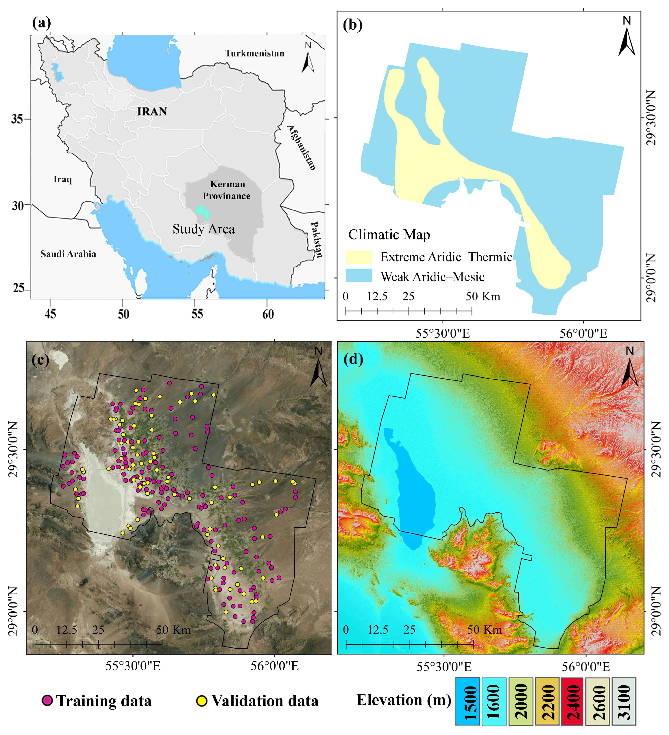
2.1. Study Area

The field of study is located between 55°05′46.7″ to 56°05′14.4″ east longitude and 28°55′15.8″ to 29°46′55.05″ north latitude, for about 50,000 ha, in arable (mainly under pistachio cultivation), as well as barren and marginal, lands of Sirjan Playa, in Kerman Province in the southeast of Iran (Figure 1a). Sirjan Playa is one of the largest playas in the Isfahan watershed, covering 1625 km² [58]. The climatic regime was identified as ranging from extreme aridic–thermic to weak aridic–mesic using the JNSM (Java Newhall Simulation Model) software, version 1.6.0 (Figure 1b). The annual average precipitation is about 172 mm and the average temperature is 16 °C. The average elevation of the area is approximately between 1500 and 3100 m above sea level (Figure 1d).

Climate plays a key role in the formation of gypsiferous soils, which primarily occur under aridic, xeric, and ustic soil moisture regimes and across various soil temperature regimes, including hyperthermic, thermic, and mesic conditions [11]. The depth distribution of gypsum content in soils depends on the prevailing climatic conditions. In strongly arid climates, the upward movement of gypsum dominates, leading to its accumulation in the epipedon (surface horizon). Conversely, in weakly arid climates, downward occurrence is more typical, resulting in gypsum accumulation in the subsurface horizons [59].

The agricultural soils in this area are classified [60] into the Aridisol order, and belong to the Gypsid and Salid suborders. The presence of saline playa deposits and gypsiferous soils aggravates the degradation of agricultural lands in the area. As the Sirjan Playa dehydrates toward the center with a slightly lower slope, the top crust becomes progressively dominated by Halite (NaCl), which is enriched in the top sediments due to capillary rise, whereas the concentration of gypsum increases along the boundary.

Soil Sampling

A total of 242 topsoil elementary sampling units (ESUs), at a depth from 0 to 15 cm, were collected in August 2023 (Figure 1c). For this purpose, the entire area was divided into heterogeneous segments, selected based on different characteristics, including geological maps, geomorphological surfaces, land use, elevation, slope, and soil moisture and temperature regimes. This segmentation was based on the assumption that these factors impact the spatial variability of gypsum content across the study area. The selected sampling strategy aimed to ensure comprehensive spatial coverage (Figure 1), thereby providing a robust asset for the model calibration in mapping gypsum content. The sampling density was adapted to the degree of heterogeneity within each segment, with more intensive sampling conducted in areas exhibiting greater environmental complexity. Each ESU consisted of five subsamples randomly selected from a 30 × 30 m area within each grid cell. These subsamples were thoroughly mixed in equal proportions to form a composite sample, from which the gypsum content was measured. This compositing approach provided a more representative estimate of gypsum for each grid cell.

2.2. Methodology

Figure 2 depicts the flowchart of the approach we have defined for estimating soil gypsum abundance over the Sirjan Playa test site. The flow chart is diffusely described in the following sub-paragraphs.

2.3. Data Gathering

2.3.1. Laboratory Analyses

After field collection, soil samples were air-dried, well crushed, and passed through a 2 mm sieve. The total amount of gypsum was measured using acetone precipitation, and electrical conductivity was measured in saturated extract [60].

2.3.2. Laboratory VNIR-SWIR Spectroscopy and Preprocessing

Spectrometry of the air-dried samples was carried out in a dark room by a Fieldspec-3-ASD spectroradiometer (Analytical Spectral Devices Inc., Boulder, CO, USA) in the 350–2500 nm wavelength interval. A contact probe equipped with an internal 6.5 W halogen light source was used for spectral measurements. The probe was designed such that the light source was vertically positioned 4.5 cm above the sample surface, the distance between the sample and the sensor was 3 cm, and both the illumination and viewing angles were fixed at 30°. The radiometer bandwidth and spectral resolutions of the ASD spectroradiometer were 1.4 and 3 nm for the visible and near-infrared (VNIR) portion (350–1000 nm) and 2–10 nm for the short-wave infrared (SWIR) portion (1000–2500 nm), respectively. ASD internal dark current and external white reference calibrations were carried out for each of five samplings (within a 15 min interval). The calibration process was repeated systematically throughout the duration of the measurements to map any changes in the boundary conditions. Each spectrum was recorded with a sampling time of 0.1 s, and up to 25 measurements per second were captured continually to generate the final spectrum for each sample. The reflectance spectra were recorded at five positions on each sample.

A series of preprocessing operations were applied to eliminate instrument-induced noise and correct spectral distortions. Splice correction was performed to address discontinuities occurring between sensors at 1000 nm and 1830 nm. To reduce illumination inconsistencies and instrument-related noise, a Savitzky–Golay smoothing filter (3rd-degree polynomial, frame size of 7) was applied to all reflectance spectra. Finally, a representative spectral signature for each sample was obtained by calculating the arithmetic mean of five preprocessed spectra.

2.3.3. Remote Sensing Data

In this research, the performances of PRISMA and EnMAP were evaluated and compared for the quantitative retrieval of gypsum content to spectra measured in laboratory settings. The Italian Space Agency (ASI) launched the hyperspectral PRISMA satellite on 22 March 2019, with a temporal resolution of 29 days (shorter revisit times of up to 7 days using the roll maneuver). The German Aerospace Center (DLR) launched the hyperspectral EnMAP sensor on 1 April 2022, with a 27-day revisit time. Both sensors have a swath width of 30 km and employ the push-broom technique with a prism-based dual-spectrometer to scan the Earth’s surface.

Table 1. Principal attributes and noisy bands of the hyperspectral imagers considered in this research.

	Sensor	Band	FWHM (nm)	Spatial Res. (m)	SNR	SNR Conditions	Bad Bands (nm)
PRISMA	VNIR 406–978 nm	63	~12	~30	>200:1 in 400–1000 nm >600:1 @ 650 nm	Nadir-looking, 30° sun zenith angle, 0.3 Earth albedo	406–468, 977–979
							1339–1459, 1793–1993, 2357–2393
	SWIR 943–2497 nm	171			>200:1 in 1000–1750 nm >100:1 in 1950–2350 nm >400 @ 1550 nm
					>200 @ 2100 nm
	PAN 400–750 nm	1	-	5	>240:1	-	-
EnMAP	VNIR 418–993 nm	91	~6.4	~30	>500 @495 nm	Nadir-looking, 30° sun zenith angle, 0.3 Earth albedo	-
	SWIR 900–2445 nm	133	~10		>150 @2200 nm		1104–1163, 1318–1472, 1967–2023, 2422–2445

summarizes the main characteristics of these two hyperspectral imagers [37,39,61,62,63,64].

Hyperspectral Satellite Data Preprocessing

For this study, a total of ten images from the PRISMA Level-2D (L2D) and EnMAP Level-2A (L2A) products were downloaded from the ASI website (https://prisma.asi.it, accessed on 19 November 2024) and the DLR website (https://eoweb.dlr.de/egp, accessed on 30 November 2024), encompassing the same timeframe. The PRISMA acquisition dates were from 10 October 2023 to 19 November 2024, while the EnMAP acquisition occurred from 25 September 2023 to 30 November 2024. PRISMA Level-2D (L2D) and EnMAP Level-2A (L2A) images were automatically processed by their respective ground segments with atmospheric correction for land surfaces as part of their standard Level-2 processing chains [63,64]. Clear-sky EnMAP Level-2A images were acquired and did not require any further corrections. For PRISMA data, which still contained pixel-level discrepancies in the geometric registration of the L2D Level, an automatic geo-registration procedure was applied using the AROSICS (Automated and Robust Open-Source Image Co-Registration Software) algorithm (https://github.com/GFZ/arosics, accessed on 19 November 2024). This algorithm utilizes the closest Sentinel-2 image as a reference to ensure co-registration with an RMS error of approximately 0.5 pixels. Spatial resampling was performed using the nearest-neighbor method. PRISMA and EnMAP images were subsequently smoothed using the Savitzky–Golay filter (with a frame size of 7 and a 3rd-degree polynomial).

Atmospheric absorbers such as water vapor and carbon dioxide exhibit significant absorption features in the 0.9-to-2.5-micrometer wavelength range. To address this issue, bands affected by residual atmospheric absorption were excluded from the analysis based on predefined masking thresholds, as detailed in Table 2. In addition to removing bands affected by atmospheric attenuation, bands that exhibited spectral overlap between the VNIR and SWIR regions, resulting in poor SNR, were also excluded, leading to the removal of 61 bands in PRISMA and 42 bands in EnMAP.

As the current study aimed to monitor gypsiferous soils using the available images, multi-date mosaics were used. Therefore, for images with overlapping areas, the mean ESU reflectance spectra were considered.

Bare-Soil Pixel Selection

The selection of bare-soil pixels is a crucial step, since it influences the amount and quality of samples used in the creation and assessment of estimating models. Bare-soil pixels were extracted by masking built-up areas, photosynthetic vegetation, and non-photosynthetic vegetation. Pixels with a normalized difference vegetation index (NDVI) higher than 0.2 were excluded from processing. The normalized cellulose absorption index (nCAI) was employed for masking non-photosynthetic vegetation. Table 2 presents the selected bands from PRISMA and EnMAP imagery, in accordance with the work of Daughtry [65]. The work of Mzid [39] proposed a threshold of 0.03, while Ward [43] suggested a lower threshold of 0.014. Ultimately, 0.02 was selected as the threshold value for this study. Table 2 shows the mathematical formulation of these indices and the associated wavelengths for each sensor. In addition, clouds, shadows, built-up areas, and other non-bare ground pixels were removed. Finally, a mosaic of PRISMA and EnMAP images was generated by calculating the average of all bare-soil spectra acquired for each pixel in the case of multiple acquisitions.

Table 2. Details of the indices and the associated wavelengths used for the two sensors.

Index	Equation	PRISMA	EnMAP	Reference
NDVI	${\displaystyle \frac{\left(p_{NIR}+p_{RED}\right)}{\left(p_{NIR}+p_{RED}\right)}}$	RRed = 664.9 nm	RRed = 679.7 nm	[66]
		RNIR = 849.2 nm	RNIR = 816.6 nm
nCAI	${\displaystyle \frac{0.5\times \left(p_1+p_2\right)-p_3}{0.5\times \left(p_1+p_2\right)+p_3}}$	P1 = 2044.7 nm	P1 = 2041.8 nm	[39,67]
		P2 = 2206.8 nm	P2 = 2216.3 nm
		P3 = 2119.2 nm	P3 = 2095.7 nm

Table 2. Details of the indices and the associated wavelengths used for the two sensors.

Index	Equation	PRISMA	EnMAP	Reference
NDVI	${\displaystyle \frac{\left(p_{NIR}+p_{RED}\right)}{\left(p_{NIR}+p_{RED}\right)}}$	RRed = 664.9 nm	RRed = 679.7 nm	[66]
		RNIR = 849.2 nm	RNIR = 816.6 nm
nCAI	${\displaystyle \frac{0.5\times \left(p_1+p_2\right)-p_3}{0.5\times \left(p_1+p_2\right)+p_3}}$	P1 = 2044.7 nm	P1 = 2041.8 nm	[39,67]
		P2 = 2206.8 nm	P2 = 2216.3 nm
		P3 = 2119.2 nm	P3 = 2095.7 nm

2.4. Parametric and Non-Parametric Regression

According to the data flow of Figure 2, three types of retrieval were tested: narrowband indices, absorption feature parameters, and ML algorithms.

2.4.1. Narrowband Spectral Indices

In this research, narrowband hyperspectral indices were computed using three arithmetic formulas suggested by Nawar et al. [49], consisting of the normalized differenced gypsum ratio (NDGI), ratio soil index (RSI), and difference soil index (DSI), to achieve the optimal band pairs related to estimating gypsum. The index structures for gypsum quantification were as follows (Equations (1)–(3)):

$$NDGI={\displaystyle \frac{{\rho }_{\lambda 1}-{\rho }_{\lambda 2}}{{\rho }_{\lambda 1}+{\rho }_{\lambda 2}}}$$

(1)

$$RSI={\displaystyle \frac{{\rho }_{\lambda 1}}{{\rho }_{\lambda 2}}}$$

(2)

$$DSI={\rho }_{\lambda 1}-{\rho }_{\lambda 2}$$

(3)

where ρ and λ are the reflectance and the wavelengths, respectively. For this purpose, all possible two-band combinations, after the images’ pre-treatment, for PRISMA (173 bands, 29,929 indices), EnMAP (182 bands, 33,124 indices), and ASD (2151 bands, 4,626,801 indices) were investigated. For each two-band combination, the coefficient of determination (R²) between the so-calculated indices and the gypsum content was assessed.

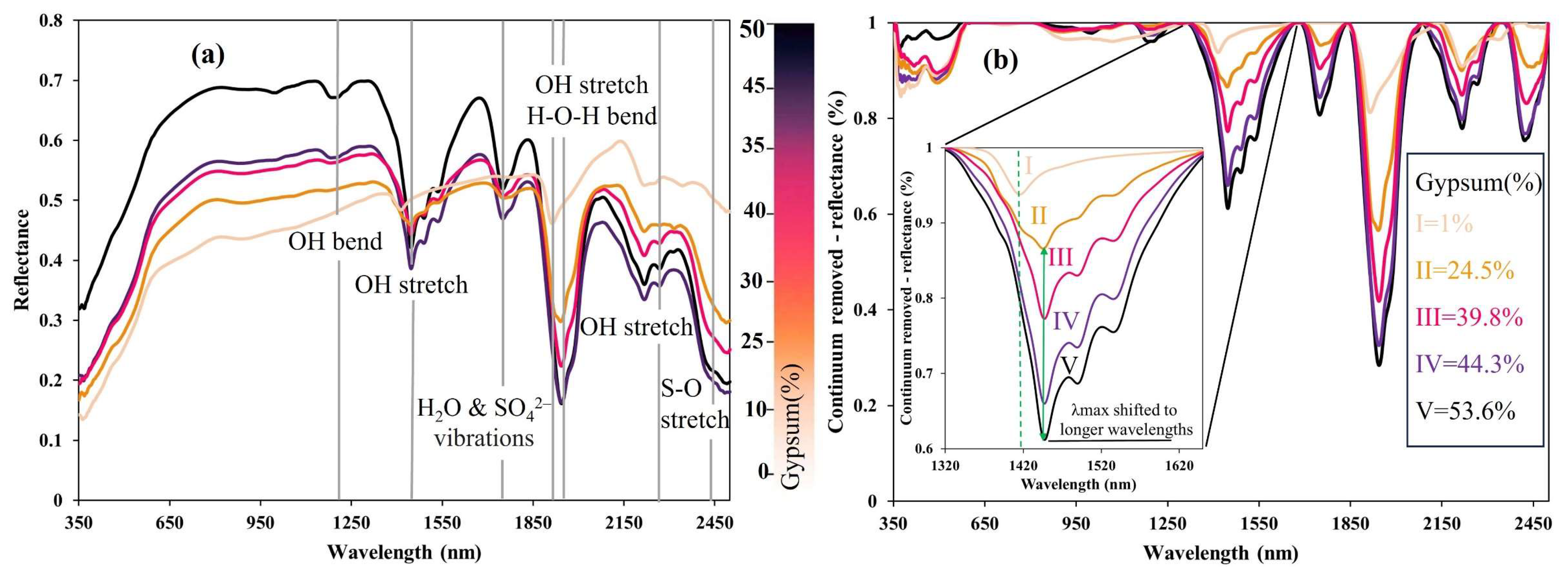
2.4.2. Gypsum Absorption Feature Parametrization

A mathematical parameterization of spectral AFs could be complex due to the occurrence of spectral confounding elements. These confounding elements could be related to interference with other spectral features, as well as the presence of atmospheric residual effects that can hide the spectral behavior of interest. On the transformed continuum removal (CR) spectrum, two parametrizations were defined. The half-area parameter (HAP) was defined with two formulations (see Figure 3). The first is the right-hand side of the surface area above 1450 nm (RHAP_1450nm), and the second is the left-hand side centered at 1750 nm (LHAP_1750nm). Furthermore, as shown in Figure 3, two parameters were defined to describe the spectrum slope. The slope parameter (SLP) is defined as the gradient when the right (RSLP_{1450–1670nm}) and left (LSLP_{1690–1750nm}) sides of the absorption feature occurring between 1450 and 1670 nm, and between 1690 and 1750 nm, respectively, are fitted linearly (Figure 3). The HAP and SLP are expressed as the following equations:

$$\text{half-area}={\int }_a^{b}f\left(x\right)dx\approx {\displaystyle \frac{b-a}{2N}}{\sum }_{n=1}^N(f(x_n)+f\left(x_{n+1}\right))$$

(4)

$$\mathrm{slope}={\displaystyle \frac{\sum _{i=1}^1(x_i-x)(r_i-r)}{\sum _{i=1}^n{(x_i-x)}^2}}$$

(5)

Equation (4) occurs in the spectral CR domain, with the zero-scaled and inversed reflectance $f$ at a wavelength x with n + 1 evenly spaced points, where n is the number of bands between the right shoulder a = 1670 nm and absorb(max) at b = 1450 nm, as well as the left shoulder a = 1690 nm and the absorb(max) at b = 1750 nm. In Equation (5), r and x are the reflectance and wavelength of the bands between 1450 nm and 1670 nm, and between 1690 nm and 1750 nm, correspondingly [68]. Figure 3 shows CR spectra of gypsum diagnostic AFs for a sample (Lat. 29.47°N, Lon. 55.46°E) with 55% gypsum.

2.4.3. Learning Algorithms

Machine learning models, including PLSR, RF, SVR, and GPR were employed for gypsiferous soil mapping based on their demonstrated ability to effectively handle spatial data and model complex relationships within the dataset [19,69,70].

PLSR is an appropriate method to address the collinearity problem across bands in hyperspectral data. It is a covariance-based strategy that aims to optimize both the explained variance and the correlation between the response variables [71]. RF can handle non-linear relationships, high-dimensional data, and feature interactions. The concept uses an iterative procedure to generate several trees using a random subset of training data. It is resilient to missing values and overfitting. This makes it appropriate for applications with incomplete and noisy data [72]. SVR is a powerful regression analysis method. It has proven to be particularly operational in managing dimensionality when datasets are limited [73]. SVR is a non-linear regression method with low computation costs and relatively high accuracy. It is founded on the premise of structural risk minimization and statistical learning theory [74]. The basis of this method is to ascertain the ideal hyperplane that minimizes error while best accommodating data points [75]. GPR is a versatile and supervised method for modeling intricate relationships in data and making forecasts with associated uncertainty. Instead of generating a single function, this approach yields a distribution over all possible functions consistent with the training data. GPR is an example of an up-to-date regression technique. It has attracted attention due to its ability to capture a wide variety of system behaviors through covariance functions [76].

The spectral reflectance data, smoothed and cleaned by the residual noisy bands (as detailed in Table 2), were used to train the machine learning algorithms. To optimize model performance, hyperparameter tuning was conducted using a grid search approach. The parameter ranges for the grid search were selected to cover a broad spectrum of potential values. The search space was discretized into a grid, and each combination was evaluated using 10-fold cross-validation. The configuration yielding the highest performance was selected as the optimal setting for model training. The explored parameter ranges and their corresponding optimal values are presented in

Table 3. Hyperparameter tuning process for PLSR, GPR, RF, and SVR algorithms.

PLSR	Parameter	Number of components
	Range	1–30
	Tuned	20
GPR	Parameter	BasisFunction	KernelScale	KernelFunction
	Range	‘constant’, ‘none’, ‘linear’, ‘pureQuadratic’	0.001–1000	‘exponential’, ‘matern32’, ‘matern52’, ‘ardsquaredexponential’
	Tuned	‘pureQuadratic’	16	“ardsquaredexponential”
RF	Parameter	NumLearningCycles	Method	MaxNumSplits	MinLeafSize
	Range	20–500	Bag, LSBoost	1–40	1–40
	Tuned	100	LSBoost	10	14
SVR	Parameter	Gamma	C	Kernel type
	Range	0.001–100	0.001–100	Gaussian, Linear, Quadratic, Cubic, RBF
	Tuned	1	10	RBF

. All model implementations and hyperparameter tuning procedures were performed using MATLAB R2024a. For the PLSR model, evaluation across a range of 1 to 30 components identified 20 as the optimal number for accurate gypsum content retrieval. In the case of the SVR model, the optimal gamma and C parameters were determined to be 1 and 10, respectively. A relatively large gamma value restricts the area of influence of each support vector to itself, which may result in overfitting, as even strong regularization via the C parameter may not sufficiently generalize the model. Conversely, a very small gamma value overly constrains the model, limiting its ability to capture complex patterns in the data and potentially leading to underfitting. For the GPR model, the optimal KernelScale parameter was determined to be 16, based on an evaluation within the range of 0 to 1000. In the case of the RF model, the optimal MinLeafSize was selected as 14 from a tested range of 1 to 40.

2.5. Model Training and Validation

Narrowband indices, the area and slope parameters describing the gypsum AFs, and the ML models were calibrated/trained and validated using the same training and test datasets. To confirm the models’ accuracy, the dataset was randomly split into ~66% for training and ~34% for testing/validation using a random holdback cross-validation approach. The accuracy of each model was evaluated using several performance criteria, incorporating the determination coefficient (R²), root mean square error (RMSE), ratio of performance to interquartile range (RPIQ), and ratio of performance to deviation (RPD), calculated as follows:

$${\mathrm{R}}^2={\displaystyle \frac{{\sum }_{i=1}^n{\left({\widehat{x}}_{i }-\overline{x}\right)}^2}{{\sum }_{i=1}^n{\left(x_i-\overline{x}\right)}^2}}$$

(6)

$$\mathrm{R}\mathrm{M}\mathrm{S}\mathrm{E}=\sqrt{{\displaystyle \frac{\sum _{\mathrm{i}=1}^{\mathrm{n}}{\left({\widehat{x}}_{i }-x\right)}^2}{\mathrm{n}}}}$$

(7)

$$\mathrm{R}\mathrm{P}\mathrm{I}\mathrm{Q}={\mathrm{Q}}_3-{\mathrm{Q}}_1/\mathrm{R}\mathrm{M}\mathrm{S}\mathrm{E}$$

(8)

$$\mathrm{R}\mathrm{P}\mathrm{D}={\displaystyle \frac{\mathrm{S}\mathrm{D}}{\mathrm{R}\mathrm{M}\mathrm{S}\mathrm{E}}}$$

(9)

The variables $x$, $\widehat{x}$, and $\overline{x}$ represent the measured, predicted, and average observed values, respectively, over n measurements. The first and third quartiles of the validation set are denoted by Q3 and Q1, respectively, while SD is the standard deviation. We used RPIQ and RPD threshold values that are commonly used in the soil spectroscopic literature to evaluate the soil prediction models’ accuracy [75,77,78,79]. Regarding RPIQ, five groups were chosen: RPIQ > 2.5 (excellent prediction), 2.0 ≤ RPIQ ≤ 2.5 (very good prediction), 1.7 ≤ RPIQ < 2.0 (good prediction), 1.4 ≤ RPIQ < 1.7 (fair prediction), and RPIQ < 1.4 (very poor prediction) [77,78]. The categories of RPD were defined as follows: RPD < 1 (very poor model prediction), 1.0 < RPD < 1.4 (poor prediction), 1.4 < RPD < 1.8 (fair prediction), 1.8 < RPD < 2.0 (good prediction), 2.0 < RPD < 2.5 (very good prediction), and RPD > 2.5 (excellent prediction) [75,79].

3. Results

3.1. General Statistics

The gypsum content statistics of the remaining bare-soil samples are presented in

Table 4. Descriptive statistics of the ESU datasets (%).

Variable	N	Min	Max	Mean	Kurtosis	Skewness	Std.	Coef. Var. (%)	KS
Whole dataset	242	0.1	55.0	8.22	1.92	1.77	14.06	171.0	0.310 **
Training set	160	0.1	55.0	7.58	2.64	1.94	13.69	180.1	0.322 **
Test set	82	0.1	50.1	9.48	1.03	1.52	14.75	155.5	0.305 **

N, Std., Coef. Var., and KS are the number of soil samples, the standard deviation, the coefficient of variation, and the statistics of the Kolmogorov–Smirnov normality test, respectively. ** show significant (p < 0.01) differences compared to the normal distribution.

. We divided the whole dataset (n = 242) into a training set (n = 160, corresponding to 66% of the whole soil samples) and a validation set (n = 82, 34% of the whole samples). Table 4 presents the main statistics for the gypsum abundance in % of the ESU for the entire dataset, training set, and validation set. The values of gypsum varied in the range of 0.1 to 55%, with a mean of 8.22%. According to the lowest and highest gypsum abundance values, the soil types in the research region range from non-gypsiferous to gypsum-rich. The high values of the coefficient of variation (CV) of more than 100% illustrate high spatial variability of gypsum in the area, based on Wilding’s [80] classification of variability into three categories according to CV values: low (CV > 15%), medium (15% < CV < 35%), and high (CV > 35%). The Kolmogorov–Smirnov (KS) normality test revealed that both the validation and calibration datasets did not follow a normal distribution (Table 4).

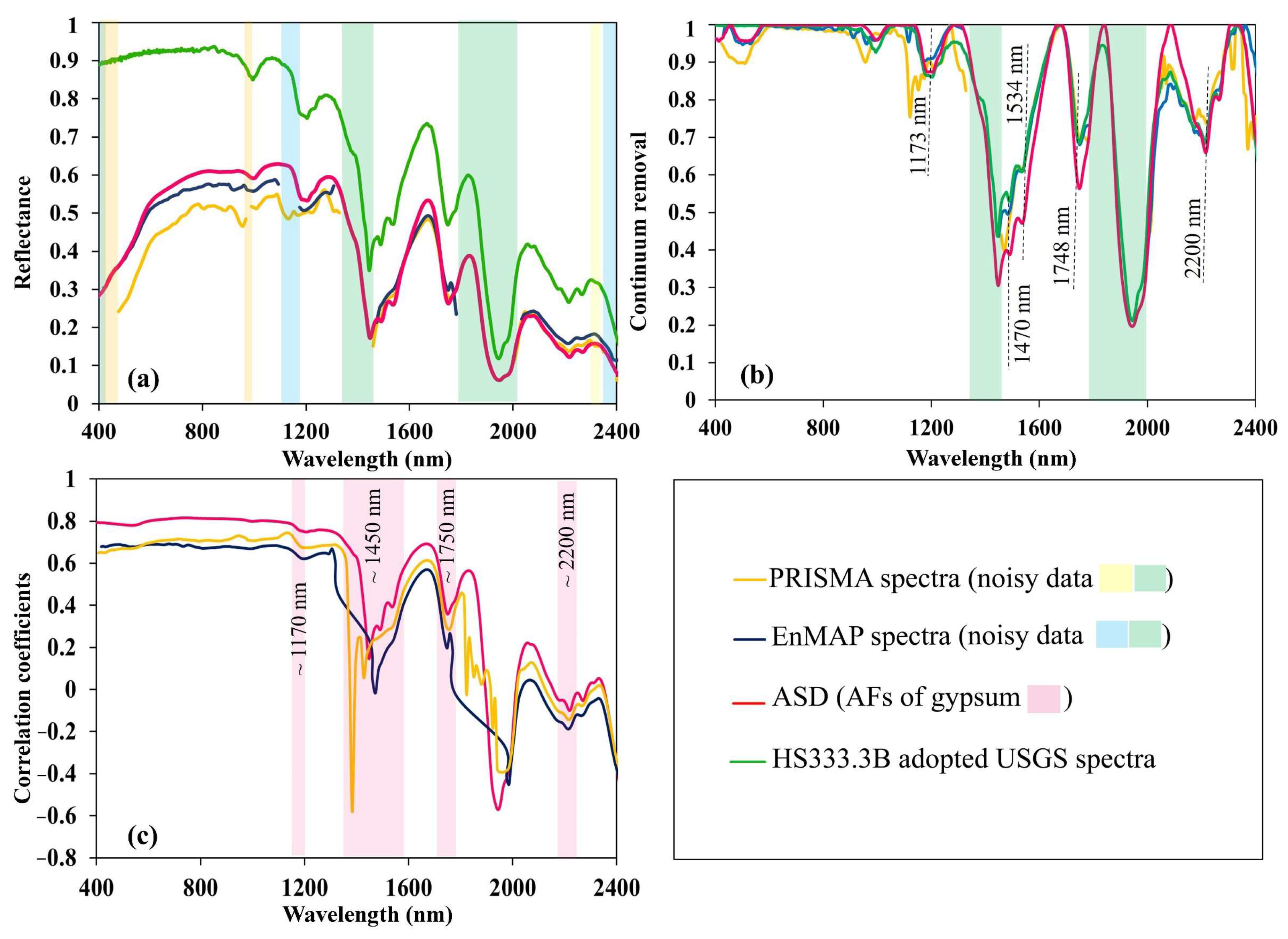
3.2. EnMAP/PRISMA Spectral Quality for Gypsum Study

To highlight the most prominent spectral properties of gypsum, sample laboratory ASD spectra with high and low gypsum contents are illustrated in Figure 4, demonstrating how varied levels of gypsum influence the sample spectral reflectance. The findings reveal that gypsum has a significant influence on reflectance, increasing it in the 350–1200 nm range, while decreasing the overall reflectance in the 1750–2500 nm range (Figure 4a). The spectra of Figure 4a show high albedo in the visible region due to a high presence of gypsum, which led to high reflectivity. The samples containing the largest quantity of gypsum display sharp distinctive spectral characteristics at 1100 nm and 1750 nm.

These features are coupled with the diagnostic finger-shaped absorption patterns in the spectrum between 1400 nm and 1500 nm, which are associated with the di-hydrated gypsum mineral (CaSO₄. 2H₂O). Given that the SWIR bands are dependent on relative humidity, a systematic trend of increasing band depth is observed for any features in samples with hydrated Ca-sulfates, which relates to the combination of O–H stretches, H–O–H bends, and various overtones [26]. Furthermore, when the amount of gypsum increases significantly, the maximum reflectance (λ_max) at 1400 nm and 1900 nm shifts to longer wavelengths, resulting in a remarkable shift in λ_max position, corroborating the conclusions stated by Rasooli et al. [30].

In Figure 5, the EnMAP/PRISMA spectra of an ESU (Lat. 29.47°N, Lon. 55.46°E) with 55% gypsum are compared with ASD spectra and the USGS (United States Geological Survey) sample (HS333.3B) depicting pure gypsum spectra. The visual comparison demonstrates good agreement between the EnMAP/PRISMA spectra and both the ESU laboratory spectrum and the USGS reference gypsum spectra (Figure 5a,b). Diagnostic absorption bands related to gypsum are located around 1450 nm, 1750 nm, and 2200 nm, with minor absorptions around 1100 nm [26]. The results show that EnMAP has successfully resolved the multiple characteristic features related to gypsum at ~1100 and ~1550 nm (Figure 5b). A significant difference was observed in the gypsum features at 1100 nm in the PRISMA-L2D spectra, which could be related to the residual effects in the atmospheric correction procedure (Figure 5b). Notably, the EnMAP/PRISMA-derived soil spectra cannot completely rely on the unique AFs centered at 1450 and 1750 nm, as the left side of AF ~1450 nm and the right side of AF ~1750 nm fall within the atmospheric attenuation bands.

Figure 5b shows that the Pearson correlation between soil reflectance and gypsum abundance has a common pattern for both the satellite imagery (PRISMA/EnMAP) and the ASD data. Among the three main gypsum AFs (at 1450 nm, 1750 nm, and 2200 nm), the most significant correlation belongs to 1750 nm (ASD shows a r = 0.40) (Figure 5c). The spectral features at 1450 nm, which lie in the water vapor absorption range, and the feature at 2200 nm, which falls in the absorption range of clay minerals, pose challenges for reliable gypsum estimation.

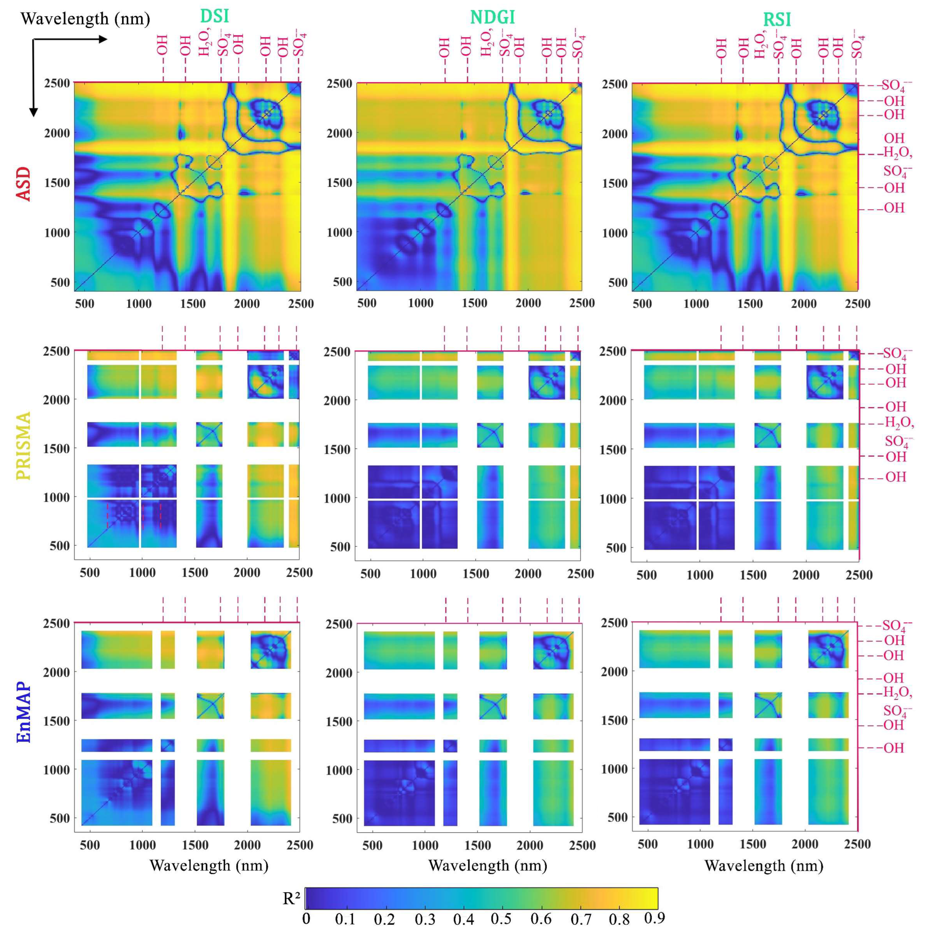
3.3. Gypsum Retrieval Using Narrowband Spectral Indices

Figure 6 presents two-correlogram plots of the R² statistics for the DSI, NDGI, and RSI narrowband indices for gypsum content retrieval using ASD, PRISMA, and EnMAP imagery. The laboratory spectroscopy results highlight the ideal conditions, such as minimal atmospheric attenuation, proper illumination, and high spectral resolution, under which spaceborne hyperspectral imagery can achieve maximum accuracy and deliver more meaningful results. This is due to the different conditions during spectral acquisition. Laboratory samples are air-dried, crushed, and sieved, and then measured under stable illumination using an artificial light source, which minimizes variability and spectral noise. In contrast, satellite sensors scan the undisturbed soil surface, where moisture, soil crusts, dry residues, temperature, and surface roughness introduce considerable spectral noise and reduce prediction accuracy. Therefore, it is expected that satellite-based prediction models generally show lower accuracy than those based on laboratory data [81,82].

The optimum index–band combinations were computed and are given in

Table 5. Comparison of three narrowband indices (DSI, NDGI, and RSI) in ASD, PRISMA, and EnMAP. The best-performing indices are shown in bold.

	Dimensions	Optimal Band Pair	R2	RMSE (%)	Equation
ASD	$2151\times$ 2151	DSI (λ1383, λ2484)	0.96	2.84	$Gypsum=118.2\times ({\mathsf{\rho }}_{\mathsf{\lambda }1383}-{\mathsf{\rho }}_{\mathsf{\lambda }2484})-2.4$
		NDGI (λ2400, λ2435)	0.93	3.67	$Gypsum=467.45\times {\displaystyle \frac{({\mathsf{\rho }}_{\mathsf{\lambda }2400}-{\mathsf{\rho }}_{\mathsf{\lambda }2435})}{({\mathsf{\rho }}_{\mathsf{\lambda }2400}+{\mathsf{\rho }}_{\mathsf{\lambda }2435})}}-6.69$
		RSI (λ2400, λ2435)	0.94	3.31	$Gypsum=206\times {\displaystyle \frac{\left({\mathsf{\rho }}_{\mathsf{\lambda }2400}\right)}{\left({\mathsf{\rho }}_{\mathsf{\lambda }2435}\right)}}-212$
PRISMA	$173\times$ 173	DSI (λ1534, λ2167)	0.79	6.88	$Gypsum=424.6\times ({\mathsf{\rho }}_{\mathsf{\lambda }1534}-{\mathsf{\rho }}_{\mathsf{\lambda }2167})-6.27$
		NDGI (λ2400, λ2435)	0.73	7.77	$Gypsum=96.02\times {\displaystyle \frac{({\mathsf{\rho }}_{\mathsf{\lambda }2400}-{\mathsf{\rho }}_{\mathsf{\lambda }2435})}{({\mathsf{\rho }}_{2400}+{\mathsf{\rho }}_{\mathsf{\lambda }2435})}}-25.68$
		RSI (λ2400, λ2435)	0.72	7.87	$Gypsum=178.19\times {\displaystyle \frac{\left({\mathsf{\rho }}_{\mathsf{\lambda }2400}\right)}{\left({\mathsf{\rho }}_{\mathsf{\lambda }2435}\right)}}-199$
EnMAP	$182\times$ 182	DSI (λ1564, λ1769)	0.84	5.90	$Gypsum=435.26\times ({\mathsf{\rho }}_{\mathsf{\lambda }1564}-{\mathsf{\rho }}_{\mathsf{\lambda }1769})-3.6$
		NDGI (λ2369, λ2407)	0.80	6.53	$Gypsum=222.84\times {\displaystyle \frac{({\mathsf{\rho }}_{\mathsf{\lambda }2369}-{\mathsf{\rho }}_{\mathsf{\lambda }2407})}{({\mathsf{\rho }}_{\mathsf{\lambda }2369}+{\mathsf{\rho }}_{\mathsf{\lambda }2407})}}+1.89$
		RSI (λ2369, λ2407)	0.78	6.98	$Gypsum=87\times {\displaystyle \frac{\left({\mathsf{\rho }}_{\mathsf{\lambda }2369}\right)}{\left({\mathsf{\rho }}_{\mathsf{\lambda }2407}\right)}}-84.45$

. Our study revealed that the best diagnostic band couples in the ASD data mainly corresponded to wavelengths λ₁₃₈₃–λ₂₄₈₄ nm and λ₂₄₀₀–λ₂₄₃₅ nm. For the satellite sensors, the selected wavelengths mainly relied on the band pairs λ₁₅₃₄–λ₂₁₆₇ nm and λ₂₄₀₀–λ₂₄₃₅ nm (PRISMA data), and λ₁₅₆₄–λ₁₇₆₉ nm and λ₂₃₆₉–λ₂₄₀₇ nm (EnMAP data). Among them, the optimal band pairs with the best accuracy belonged to the DSI ratio index (${\mathrm{R}}_{\mathrm{A}\mathrm{S}\mathrm{D}}^2=0.96,{\mathrm{R}}_{\mathrm{P}\mathrm{R}\mathrm{I}\mathrm{S}\mathrm{M}\mathrm{A}}^2=0.79,{\mathrm{R}}_{\mathrm{E}\mathrm{n}\mathrm{M}\mathrm{A}\mathrm{P}}^2=0.84)$ in comparison to the NDGI and RSI ratios. The maximum R² for the DSI ratio was obtained by combining bands λ₁₃₈₃ and λ₂₄₈₄ nm for ASD, bands λ₁₅₃₄ and λ₂₁₆₇ nm for PRISMA, and bands λ₁₅₆₄ and λ₁₇₆₉ nm for EnMAP (Table 5).

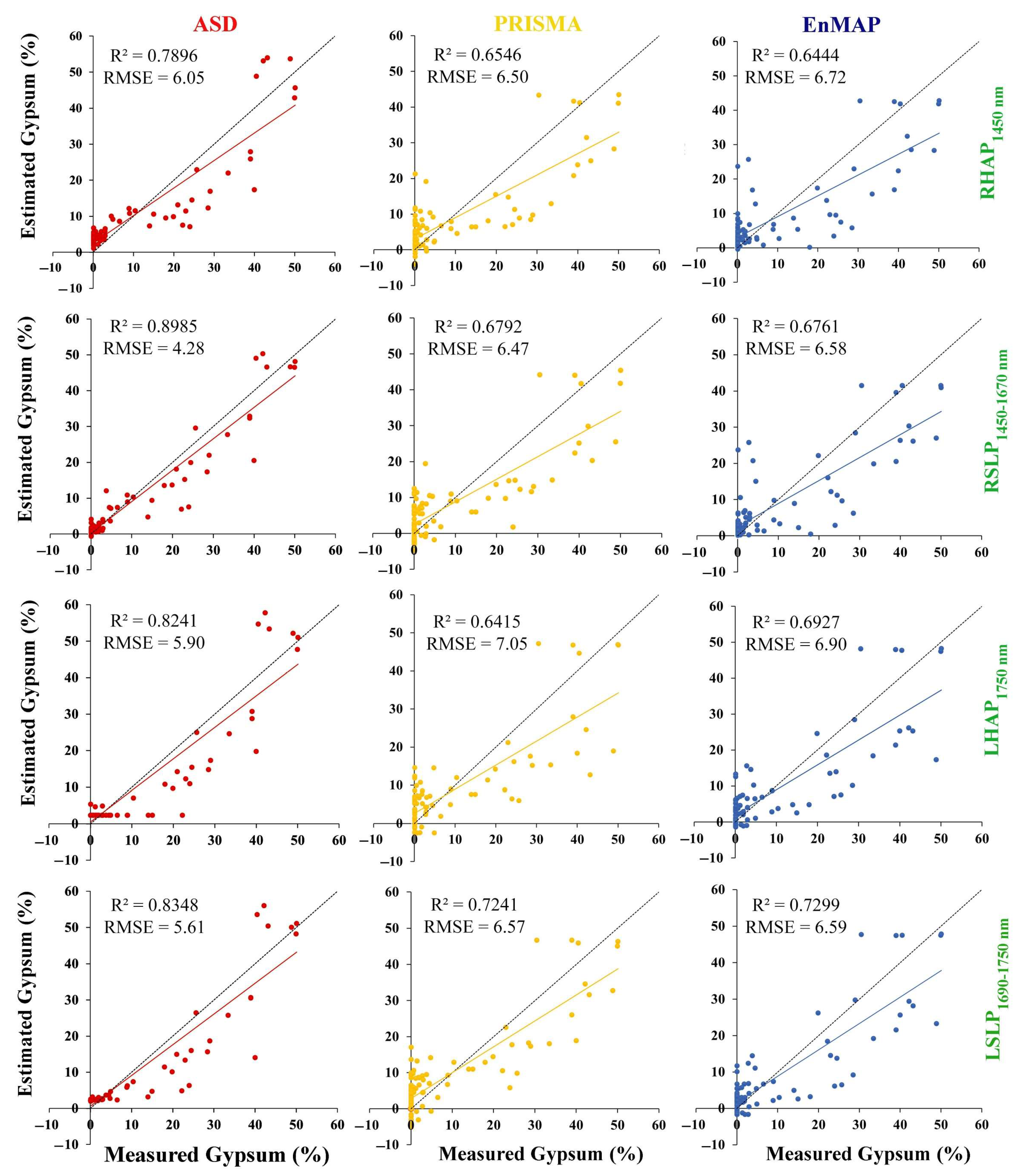
3.4. Soil Gypsum Content Retrieval Using HAP and SLP Indices

Figure 7 illustrates the exclusive performance reliance of the parametrization for gypsum content forecasting using the HAP (RHAP_1450nm and LHAP_1750nm) and SLP (RSLP_{1450–1670nm} and LSLP_{1690–1750nm}) indices.

Despite focusing on only two spectral features located at 1450 nm and 1750 nm, their spectral shapes and reflectance patterns can be applied as reliable indicators of gypsum occurrence (the R² values ranged from 0.64 to 0.89; Figure 7). The results indicate that, for all three datasets (i.e., ASD, PRISMA, and EnMAP), the SLP index exhibited more accurate gypsum estimation compared with the HAP index, as shown in Figure 7. The optimal model’s gypsum estimation using the RSLP_{1450–1670 nm} index in the validation dataset revealed R² = 0.89 and RMSE = 4.28% for ASD. For the LSLP_{1690–1750nm} index, R² = 0.72 and RMSE = 6.57% were obtained for PRISMA, and R² = 0.72 and RMSE = 6.59% for EnMAP, respectively.

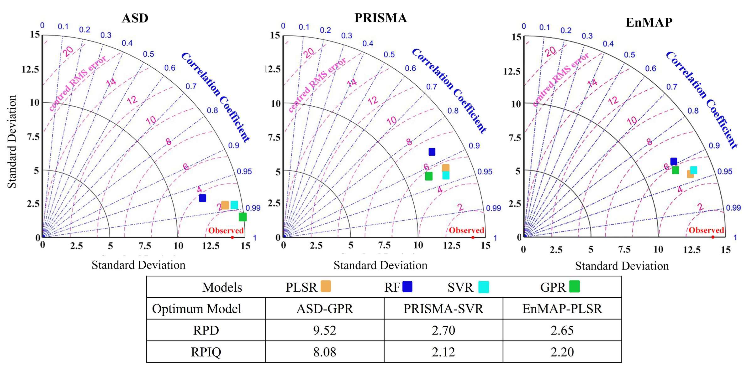
3.5. Gypsum Retrieval Using ML Algorithms

Unlike most previous research, which has focused only on the detection of gypsum in soil [40,83], this study aims to predict the gypsum abundance in soil. To this end, machine learning (ML) algorithms, including PLSR, RF, GPR, and SVR, were applied. The dataset was split into two subsets for training and validation purposes: the training subset (n = 160) was used to develop the prediction models, while the validation subset (n = 82) was employed to assess the models’ performance and generalization ability. Based on the Kolmogorov–Smirnov normality test results (Table 4), neither the calibration nor the validation datasets followed a normal distribution, which might have affected the ML models’ performance. The best results for gypsum content estimation are highlighted in

Table 6. Performance of PLSR and three ML models in predicting gypsum abundance. The best-performing models are shown in bold green font.

Sensors	ASD				PRISMA				EnMAP
Model	R2	RMSE	RPD	RPIQ	R2	RMSE	RPD	RPIQ	R2	RMSE	RPD	RPIQ
PLSR	0.972	2.41	5.94	5.12	0.828	5.42	2.59	2.04	0.851	5.30	2.65	2.20
RF	0.941	3.18	4.42	3.42	0.755	6.70	2.11	1.62	0.792	6.08	2.31	1.80
SVR	0.971	2.51	5.73	4.91	0.835	5.20	2.70	2.12	0.844	5.55	2.56	2.00
GPR	0.989	1.52	9.52	8.08	0.829	5.27	2.64	2.10	0.825	5.59	2.52	2.10

.

To comprehensively evaluate the PLSR, RF, SVR, and GPR models, Taylor diagrams were employed to scrutinize the correlation coefficient, standard deviation, and RMSE values for the models (Figure 8). As can be seen, RF estimates (blue points) for all the sensors showed lower performance than the other models. Meanwhile, the PLSR, SVR, and GPR algorithms had more consistent model errors for both the ASD and satellite datasets. The results also indicate that the GPR model demonstrated a closer distance to the measured values and outperformed all other algorithms in estimating lab ASD data, with R² > 0.98 and RMSE < 1.6%. Among all models, the best gypsum prediction was achieved by SVR (RPD > 2.60, R² > 0.83, RMSE < 5.30%) on the PRISMA dataset and PLSR (RPD > 2.60, R² > 0.85, RMSE < 5.30%) on the EnMAP dataset.

4. Discussion

4.1. Evaluating Spectral Index Performance for Gypsum Content Retrieval

Narrowband approach. All three narrowband spectral indices in this study showed good performance in estimating gypsum content. Among the evaluated spectral indices, the DSI exhibited superior performance in predicting soil gypsum content compared to the NDGI and RSI (Table 5). As shown in Table 5, the most effective narrowband index combinations for both the laboratory- (ASD) and satellite-derived datasets consist of bands located in the SWIR region; since these bands are less influenced by surface soil color, they contribute to increased stability and improved discriminatory capability of the indices. The available literature also confirms that the identified spectral regions correspond to gypsum-sensitive bands. Specifically, they include the 1400–1500 nm, 1750 nm, and 2400 nm ranges, along with multiple spectral features around 2100–2300 nm associated with water molecules (H₂O) [26,27,28]. Similarly to previous studies [27,84], the selection of these useful bands can be linked to O–H stretching, H–O–H bending fundamentals, and overtone combinations (Figure 4a and Figure 6).

The computation results indicate that the indices can account for the variability in spectral reflectance across different soil pixels, leading to the identification of the most suitable wavelength pairs for gypsum assessment. However, slight variations in the selected wavelength combinations can be attributed to differences in radiometric resolution and preprocessing procedures. Notably, as shown in Figure 6, despite the presence of distinct absorption features (Figure 5), the most optimal wavelength pairs for the examined indices do not lie strictly within the 1400 and 1750 nm ranges. This observation suggests that computing optimal index–wavelength pairs across the entire spectral range enhances the detection capabilities of narrowband indices.

Spectral feature approach. The analysis of laboratory-acquired spectra demonstrated the feasibility of using such data as a reliable benchmark for satellite-based assessments (Figure 7). The reduced performance of the models when moving from ASD to satellite data suggests that atmospheric correction can alter or obscure the key absorption features of gypsum. This effect diminishes the effectiveness of the HAP index more than the SLP index, although both indices show lower accuracy for the PRISMA and EnMAP data compared to the ASD spectra. Therefore, unlike the laboratory-acquired spectra (ASD), satellite-derived soil spectra cannot fully rely on the distinct absorption features centered at 1400 and 1750 nm, as these are affected by atmospheric attenuation in the remotely sensed images. For satellite-based data, the reflectance values at the left (~1450 nm) and right (~1780 nm) shoulders of the gypsum absorption features are not useful. This is because these wavelengths are located near atmospheric absorption features caused by water vapor, which significantly reduce both incident and reflected light, thereby making the information in these spectral regions unavailable [84,85,86].

Model performance evaluation in satellite analyses indicated that PRISMA performs slightly worse than EnMAP in the LHAP_1750nm parameter. This can be attributed to the fact that the gypsum AF at 1750 nm, as well as the finger-shaped AFs around 1490 nm and 1540 nm, are relatively narrow spectral features. EnMAP, with a full width at half maximum (FWHM) of approximately 10 nm, provides finer spectral resolution compared to PRISMA, which has a FWHM of about 14 nm in the relevant spectral range. Furthermore, EnMAP’s better performance is likely also due to its higher SNR compared to PRISMA in this spectral region. Thus, this method requires high spectral resolution to precisely define the central wavelength of the absorption features, as well as the positions of the right and left shoulders, both of which are crucial for enhancing modeling efficiency and accurately predicting gypsum content. Our results are consistent with the findings of Milewski et al. [8], who extracted shape-based parameters using EnMAP simulated pre-launch data.

Furthermore, the direct quantitative prediction of soil properties using individual absorption features often faces challenges due to their non-specific nature and tendency to overlap [87]. In this study, the presence of saline soils in some sectors of the area (with EC values reaching up to 200 dS/m) (results not shown) may also have led to interference from overlapping absorption features associated with salinity near 1450 nm, potentially shifting or obscuring the characteristic gypsum absorption peaks [30]. Such spectral interference can reduce the reliability of gypsum-related indices centered around 1450 nm.

Spectral index effectiveness. Our findings indicate that the narrowband ratio is a more robust and reliable method for retrieving gypsum content compared to the AF parameters. This is because the narrow spectral feature method better eliminates speckle noise and atmospheric interference associated with wavelengths nearest to the optimal ones for gypsum. In contrast, due to the proximity of the wavelengths chosen for feature extraction indices to atmospheric absorption bands, the accuracy of gypsum concentration retrieval is reduced. Overall, computing optimal index–wavelength pairs and diagnostic AFs across the full spectrum enhances comparability between datasets and sensing platforms (e.g., when using different resolution sensors), as the most significant diagnostic features may appear in different spectral ranges on various platforms.

Overall, the accuracy of the models, as expressed by the R² for the validation sets, shows a rather satisfactory performance (Table 5, Figure 7). Interestingly, although the satellite-derived spectra are unable to fully capture all prominent absorption bands associated with gypsum features, absorption feature indices still demonstrate satisfactory performance. This observation underscores the potential of these indices, despite their traditional association with spectra exhibiting distinct absorption bands, to offer valuable insights for soil attribute analysis in satellite data. Thus, on the one hand, this result could be an indicator of the quality of EnMAP/PRISMA-derived spectra, and on the other hand, it could emphasize that spectral indices can be utilized as an exploratory method to identify defining features related to other soil properties before developing and deploying complex models. Previous studies have utilized spectral index calculation and spectral feature absorption extraction to assess the correlation between spectral data and various soil properties, including soil organic matter [88,89,90,91], heavy metals [92], gypsum content [8], soil moisture [93], salinity, and calcium carbonate [47]. The use of spectral indices reduces data volume by removing redundant information, simplifying the modeling, and assuring greater transferability due to their basis in spectrally derived material properties.

4.2. Evaluation of ML Methods for Accurate Gypsum Retrieval from Hyperspectral Data

The results clearly show that all of the ML algorithms (PLSR, RF, SVR, and GPR) in both IS sensors were effective in predicting gypsum content with reliable accuracy (RPD > 2) (Table 6). This occurred despite the inevitable reduction in SNR, highlighting the advantages of high spectral resolution in new hyperspectral sensors, particularly within the SWIR range, where key soil spectral features are concentrated. In particular, in the four examined models of Table 6, PRISMA yielded R² values ranging from 0.75 to 0.83 and EnMAP yielded values ranging from 0.79 to 0.85, thus indicating a somewhat better performance for EnMAP. By comparing Table 5 and Table 6, it can be observed that ML models developed on the whole spectrum yielded higher accuracy than parametric models. This improvement is attributed to the capability of ML algorithms to enhance predictive accuracy and relevance to soil science by learning from observational data and effectively integrating structured knowledge [94]. The results of this study support further research into feature extraction and regression applications of ML algorithms using IS and ASD data to predict gypsum and other soil properties. Advancing these approaches could enhance model performance, especially when working with large and high-dimensional datasets. The decrease in performance of the models developed on images compared with ASD data is primarily linked to the higher spectral resolution of the laboratory sensor, and secondarily attributed to the satellite dataset hiding the gypsum diagnostic features with water vapor absorption. This motivates us to pursue the approach of fusing ground spectra and new-generation hyperspectral imagers to obtain precise predictions by integrating data from multiple sensors.

The results also indicate that different algorithms exhibit varying capabilities in predicting gypsum content at unsampled locations. The difference in prediction accuracy between algorithms may be attributed to the distinct mathematical functions used by each [70,95]. Performance evaluation metrics indicate that the PLSR model has a good capability to accurately fit hyperspectral reflectance across varying levels of gypsum content. Wang et al. [96] previously demonstrated the superiority of PLSR for cases with small sizes of label data; this can be attributed to the fact that PLSR feature inputs are minimized to very few orthogonal latent components. Compared to previous studies, Ward et al. [48] and Steinberg et al. [97] achieved good prediction accuracies for selected soil properties using the PLSR method applied to simulated EnMAP imagery. In contrast, Bouslihim et al. [98] achieved higher accuracy using PRISMA data with the SVR algorithm compared to with the PLSR and RF models.

Overall, it is challenging to draw definitive conclusions regarding the effectiveness of models in predicting soil properties across different regions, as the accuracy of predictions is highly influenced by various factors, such as data variability and sampling density. Moreover, since soil spectra reflect the complex interactions among various soil constituents (e.g., mineralogy, texture, and moisture), all of which significantly influence spectral responses, the prediction accuracy of the model may decrease when applied outside the calibration area.

4.3. Assessing PRISMA and EnMAP Capabilities in Gypsum Retrieval

As demonstrated by previous studies [8,30,99] and confirmed in this research, laboratory spectroscopy data have a strong capability for gypsum content retrieval. However, the ultimate goal of this work is to scale these methods to PRISMA and EnMAP spaceborne sensors. The variability in soil conditions (particularly moisture content and roughness), atmospheric attenuation, limited SNR in some specific spectral regions, and mixing effects related to the 30 m/pixel spatial resolution can significantly impact soil property retrieval [23,100,101]. Overall, spatial resolution is critically important for successful analysis. When the sensor’s spatial resolution is lower than the variability scale on the Earth’s surface, each pixel inevitably contains a combination of multiple distinct components, which can negatively affect the quality of remote sensing data and result in poorer modeling of the target variable compared to laboratory spectral methods.

The findings of this study demonstrate that gypsum content predictions, using PRISMA and EnMAP hyperspectral data, yielded reliable results comparable to those obtained from ASD measurements. The results show slight differences in retrieval performance between PRISMA and EnMAP. Regarding the feature extraction indices, the R² values for both PRISMA and EnMAP sensors fall within a similar range of approximately 0.64 to 0.72, showing no significant difference between the two (Figure 7). In contrast, the narrowband spectral indices yielded R² values ranging from 0.72 to 0.79 for PRISMA, while EnMAP produced higher values, ranging from 0.78 to 0.84 (Table 5). For machine learning methods, the R² values range from 0.75 to 0.83 for PRISMA and from 0.79 to 0.85 for EnMAP, indicating a slight advantage for EnMAP. The lower performance of PRISMA may be attributed to the radiometric and atmospheric correction algorithm used to generate the standard L2D product delivered by the ASI. This is supported by recent findings [102,103], which also reported inconsistencies in PRISMA-derived spectra compared to those from similar platforms such as EnMAP, particularly in the SWIR region.

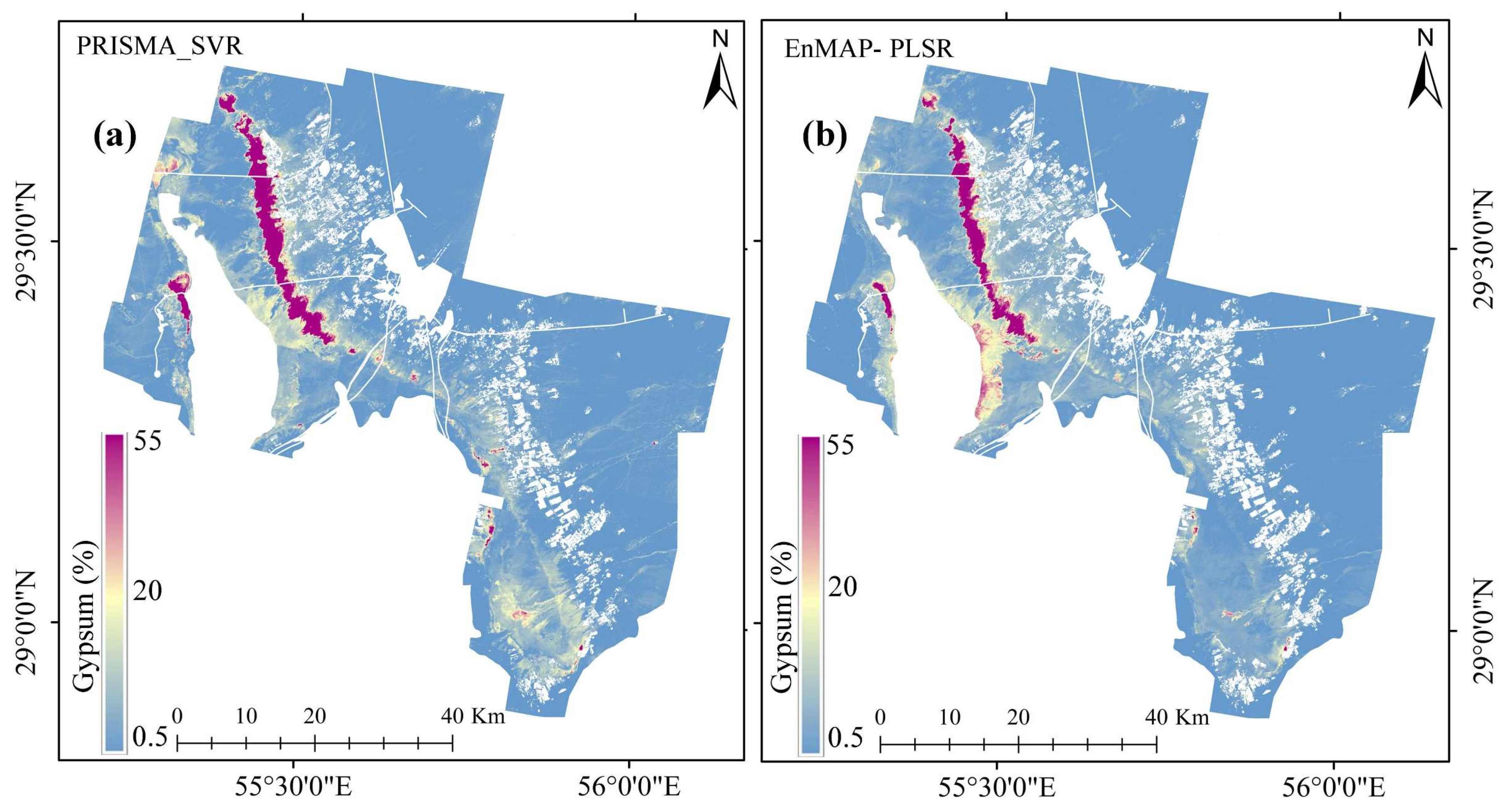
4.4. Comparative Evaluation of Gypsum Spatial Mapping Using PRISMA and EnMAP

The gypsum maps were generated using bare-soil mosaic PRISMA and EnMAP images combined with the most effective ML algorithm. The resulting gypsum maps for PRISMA (using the SVR algorithm) and EnMAP (using the PLSR algorithm) demonstrate the high quality of the products, especially in terms of dynamic range and spatial pattern (Figure 9). Soil gypsum content in the test area generally trends upward from east to west to the margin of the Sirjan Playa. The range of the predicted gypsum shows similar hotspot trends between PRISMA and EnMAP. However, marginal differences in the spatial distribution maps in PRISMA and EnMAP data could be traced back to the non-contemporary acquisition, which could have led to differences pertaining to variable soil moisture conditions. This is in accordance with the work of Milewski et al. [8], which reported how spatial and temporal variables can effectively influence the model’s operation. Over the forthcoming decade, global hyperspectral mapping missions are expected to enhance the regular availability of hyperspectral-based soil products from space, thereby opening new avenues for soil monitoring and mapping.

A visual comparison of the two maps (Figure 9) indicates that the spatial distribution of gypsum closely corresponds to the boundaries of the extremely aridic–thermic climatic zones shown on the climatic map (Figure 1b). The maps in Figure 9 show key factors in Sirjan Playa that have hampered agricultural activity: (i) the presence of gypseous soils with a high soil gypsum content (up to 55%); (ii) the formation of extremely saline land in the vicinity of this playa; and (iii) the gradual spread of salinity to marginal areas over time, as well as environmental stresses (high temperatures and low precipitation). These give a picture of topsoils that are under the threat of degradation, subject to climate change; therefore, the characterization of topsoil condition based on the abundance assessment of evaporitic mineral content is an environmental topic to be addressed.

Ultimately, the gypsum maps derived from the PRISMA and EnMAP data show noticeable similarity. This encourages us to pursue the harmonization of EnMAP and PRISMA data in future work, aiming to enhance the consistency and reliability of gypsum maps generated from multiple sensors.

4.5. Limitations and Future Work

Although the availability of data from satellite-based imaging spectroscopy sensors is steadily increasing, current missions remain limited by acquisition constraints that restrict the temporal frequency and spatial coverage of global observations. However, these limitations are expected to be mitigated with the forthcoming launches of missions such as the Copernicus Hyperspectral Imaging Mission for the Environment (CHIME, ESA) and the Surface Biology and Geology (SBG, NASA), which will offer wider swath widths and improved temporal resolution, enabling more consistent and comprehensive monitoring. Currently, PRISMA and EnMAP data are valuable for regional-scale studies in order to test and establish best practices for hyperspectral data analysis. Looking ahead, imaging spectroscopy will facilitate large-scale soil mapping efforts, particularly for the monitoring of other degradation-prone soils in arid regions, such as saline–sodic and calcareous soils, thereby supporting sustainable land management strategies. Future studies will evaluate the combination of the VSWIR hyperspectral resource with the LWIR spectral region, which could enable more detailed saline–sodic and calcareous soil characterization, as well incorporating SAR data for soil moisture assessment.

5. Conclusions

This investigation leveraged the potential of new-generation hyperspectral satellite imagers (i.e., PRISMA and EnMAP), with respect to ASD laboratory-acquired spectra, for estimating soil gypsum content. Narrowband indices (NDGI, DSI, RSI), absorption feature parameters (HAP, LSP), and ML techniques were explored and compared. The high spectral resolution of these sensors and their accuracy in retrieving the abundances of gypsum in soil were explored. ASD retrieval showed that the narrowband indices outperformed the absorption feature parameters; the DSI and RSLP_{1450–1670 nm} were identified as the best-performing indicators (R² = 0.96 and 0.89, respectively). The models tested with the PRISMA and EnMAP datasets yielded the highest accuracy for the DSI (${\mathrm{R}}_{\mathrm{P}\mathrm{R}\mathrm{I}\mathrm{S}\mathrm{M}\mathrm{A}}^2=0.78$; ${\mathrm{R}}_{\mathrm{E}\mathrm{n}\mathrm{M}\mathrm{A}\mathrm{P}}^2=0.81$) and LSLP_1750nm index (${\mathrm{R}}_{\mathrm{P}\mathrm{R}\mathrm{I}\mathrm{S}\mathrm{M}\mathrm{A}}^2=0.72$; ${\mathrm{R}}_{\mathrm{E}\mathrm{n}\mathrm{M}\mathrm{A}\mathrm{P}}^2=0.72$). This demonstrates the suitability of the proposed retrieval methods and the quality of the satellite data. Applying ML regression techniques for proximal and hyperspectral remote sensing data, exploiting the full VNIR–SWIR reflectance spectrum, improved the accuracy of gypsum modeling, achieving an R² value of over 0.98 for the laboratory ASD data. By applying the SVR and PLSR models to the remotely sensed data, high performance metrics were obtained for PRISMA (R² = 0.83, RPD = 2.70, RPIQ = 2.12) and EnMAP (R² = 0.85, RPD = 2.65, RPIQ = 2.20), respectively. Overall, the strong accordance between laboratory- and satellite-based predictions underscores the significant potential of spaceborne hyperspectral data for monitoring topsoil properties in semi-arid regions, mainly characterized by gypsum content, thus supporting broader environmental applications.

References

1. Styc, Q.; Pachon, J.; Padarian, W.; McBratney, A. Creating soil districts for Australia based on pedogenon mapping. Geoderma 2025, 454, 117164. [Google Scholar] [CrossRef]
2. GLASOD. Global Assessment of Human-Induced Soil Degradation. 1991. Available online: https://isric.org/projects/global-assessment-human-induced-soil-degradation-glasod (accessed on 1 June 2024).
3. Becker Pickson, R.; Gui, P.; Chen, A.; Boateng, E. Climate change and food security nexus in Asia: A regional comparison. Ecol. Inform. 2023, 76, 102038. [Google Scholar] [CrossRef]
4. Wang, J.; Wang, Y.; Xu, D. Desertification in northern China from 2000 to 2020: The spatial-temporal processes and driving mechanisms. Ecol. Inform. 2024, 82, 102769. [Google Scholar] [CrossRef]
5. Eisele, A.; Chabrillat, S.; Hecker, C.; Hewson, R.; Lau, I.C.; Rogass, C.; Segl, K.; Cudahy, T.J.; Udelhoven, T.; Hostert, P.; et al. Advantages using the thermal infrared (TIR) to detect and quantify semi-arid soil properties. Remote Sens. Environ. 2015, 163, 296–311. [Google Scholar] [CrossRef]
6. Chakherlou, S.; Jafarzadeh, A.A.; Ahmadi, A.; Feizizadeh, B.; Shahbazi, F.; Darvishi Boloorani, A.; Mirzaei, S. Soil wind erodibility and erosion estimation using Landsat satellite imagery and multiple-criteria decision analysis in Urmia Lake Region, Iran. Arid Land Res. Manag. 2022, 37, 71–91. [Google Scholar] [CrossRef]
7. Soil Resources, Management and Conservation Service; FAO. Management of Gypsiferous Soils; FAO Soils Bulletin 62; FAO: Rome, Italy, 1990. [Google Scholar]
8. Milewski, R.; Chabrillat, S.; Brell, M.; Schleicher, A.; Guanter, L. Assessment of the 1.75 μm absorption feature for gypsum estimation using laboratory, air- and spaceborne hyperspectral sensors. Int. J. Appl. Earth Obs. Geoinf. 2019, 77, 69–83. [Google Scholar] [CrossRef]
9. Rasooli, N.; Farpoor, M.H.; Mahmoodabadi, M.; Esfandiarpour Boroujeni, I. Genesis and distribution of different mineral assemblages controlled by environmental factors in soils and evaporitic deposits of Lut Desert, central Iran. Environ. Earth Sci. 2021, 80, 779. [Google Scholar] [CrossRef]
10. Marques, M.J.; Alvarez, A.M.; Carral, P.; Esparza, I.; Sastre, B.; Bienes, R. Estimating soil organic carbon in agricultural gypsiferous soils by diffuse reflectance spectroscopy. Water 2020, 12, 261. [Google Scholar] [CrossRef]
11. Casby-Horton, S.; Herrero, J.; Rolong, N.A. Chapter Four—Gypsum Soils—Their Morphology, Classification, Function, and Landscapes. Adv. Agron. 2015, 130, 23–81. [Google Scholar]
12. Verheye, W.H.; Boyadgiev, T.G. Evaluating the land use potential of gypsiferous soils from field pedogenic characteristics. Soil Use Manag. 1997, 13, 97–103. [Google Scholar] [CrossRef]
13. Smith, R.; Robertson, V.C. Soil and irrigation classification of shallow soils overlying gypsum beds, northern Iraq. J. Soil Sci. 1962, 13, 106–115. [Google Scholar] [CrossRef]
14. Herrero, J.; Artieda, O.; Hudnall, W.H. Gypsum, a Tricky Material. Soil Sci. Soc. Am. J. 2009, 73, 1757–1763. [Google Scholar] [CrossRef]
15. Poch, R.M.; De Coster, W.; Stoops, G. Pore space characteristics as indicators of soil behaviour in gypsiferous soils. Geoderma 1998, 87, 87–109. [Google Scholar] [CrossRef]
16. Etesami, H.; Halajian, L.; Jamei, M. A qualitative land suitability assessment in gypsiferous soils of Kerman Province, Iran. Aust. J. Basic Appl. Sci. 2012, 6, 60–64. [Google Scholar]
17. Moret-Fernandez, D.; Herrero, J. Effect of gypsum content on soil water retention. J. Hydrol. 2015, 528, 122–126. [Google Scholar] [CrossRef]
18. Porta, J. Methodologies for the analysis and characterization of gypsum in soils: A review. Geoderma 1998, 87, 31–46. [Google Scholar] [CrossRef]
19. Viscarra Rossel, R.A.; Shen, Z.; Lopez, L.R.; Behrens, T.; Shi, Z.; Wetterlind, J.; Sudduth, K.A.; Stenberg, B.; Guerrero, C.; Gholizadeh, A.; et al. An imperative for soil spectroscopic modelling is to think global but fit local with transfer learning. Earth Sci. Rev. 2024, 254, 104479. [Google Scholar] [CrossRef]
20. Demattê, J.A.; Rizzo, R.; Rosin, N.A.; Poppiel, R.R.; Novais, J.J.M.; Amorim, M.T.A.; Rodriguez-Albarracín, H.S.; Rosas, J.T.F.; dos Anjos Bartsch, B.; Vogel, L.G.; et al. A global soil spectral grid based on space sensing. Sci. Total Environ. 2025, 968, 178791. [Google Scholar] [CrossRef] [PubMed]
21. Novais, J.J.M.; Melo, B.M.D.; Junior, A.F.N.; Lima, R.H.C.; Souza, R.E.; Melo, V.F.; Amaral, E.F.; Tziolas, N.; Demattê, J.A.M. Online analysis of Amazon’s soils through reflectance spectroscopy and cloud computing can support policies and sustainable development. J. Environ. Manag. 2025, 375, 124155. [Google Scholar] [CrossRef]
22. Wang, S.; Guan, K.; Zhang, C.; Jiang, C.; Zhou, Q.; Li, K.; Herzberger, L. Airborne hyperspectral imaging of cover crops through radiative transfer process-guided machine learning. Remote Sens. Environ. 2023, 285, 113386. [Google Scholar] [CrossRef]
23. Chabrillat, S.; Ben-Dor, E.; Cierniewski, J.; Gomez, C.; Schmid, T.; van Wesemael, B. Imaging spectroscopy for soil mapping and monitoring. Surv. Geophys. 2019, 40, 361–399. [Google Scholar] [CrossRef]
24. Khosravi, V.; Gholizadeh, A.; Žížala, D.; Kodešová, R.; Saberioon, M.; Agyeman, P.C.; Vokurková, P.; Juřicová, A.; Spasić, M.; Borůvka, L. On the impact of soil texture on local scale organic carbon quantification: From airborne to spaceborne sensing domains. Soil Tillage Res. 2024, 241, 106125. [Google Scholar] [CrossRef]
25. Stenberg, B.; Viscarra-Rossel, R.A. Diffuse reflectance spectroscopy for high-resolution soil sensing. In Proximal Soil Sensing; Springer: Dordrecht, The Netherlands, 2010; pp. 29–47. [Google Scholar]
26. Hunt, G.R.; Salisbury, J.W. Visible and near-infrared spectra of minerals and rocks. II. Carbonates. Mod. Geol. 1971, 2, 23–30. [Google Scholar]
27. Cloutis, E.A.; Hawthorne, F.C.; Mertzman, S.A.; Krenn, K.; Craig, M.A.; Marciano, D.; Methot, M.; Strong, J.; Mustard, J.F.; Blaney, D.L.; et al. Detection and discrimination of sulfate minerals using reflectance spectroscopy. Icarus 2006, 184, 121–157. [Google Scholar] [CrossRef]
28. Bishop, J.L.; Lane, M.D.; Dyar, M.D.; King, S.J.; Brown, A.J.; Swayze, G.A. Spectral properties of Ca-sulfates: Gypsum, bassanite, and anhydrite. Am. Mineral. 2014, 99, 2105–2115. [Google Scholar] [CrossRef]
29. Liu, Y.; Wang, A.; Freeman, J.J. Raman, MIR and NIR spectroscopic study of calcium sulfates: Gypsum, bassanite and anhydrite. In Proceedings of the 40th Lunar and Planetary Science Conference, Houston, TX, USA, 23–27 March 2009; p. 2128. [Google Scholar]
30. Rasooli, N.; Farpoor, M.H.; Mahmoodabadi, M.; Esfandiarpour Boroujeni, I. Vis-NIR spectroscopy as an eco-friendly method for monitoring pedoenvironmental variations and pedological assessments in Lut Watershed, Central Iran. Soil Tillage Res. 2023, 233, 105808. [Google Scholar] [CrossRef]
31. Gholizadeh, A.; Žižala, D.; Saberioon, M.; Borůvka, L. Soil organic carbon and texture retrieving and mapping using proximal, airborne, and Sentinel-2 spectral imaging. Remote Sens. Environ. 2018, 218, 89–103. [Google Scholar] [CrossRef]
32. Angelopoulou, T.; Tziolas, N.; Balafoutis, A.; Zalidis, G.; Bochtis, D. Remote sensing techniques for soil organic carbon estimation: A review. Remote Sens. 2019, 11, 676. [Google Scholar] [CrossRef]
33. Castaldi, F. Sentinel-2 and Landsat-8 multi-temporal series to estimate topsoil properties on croplands. Remote Sens. 2021, 13, 3345. [Google Scholar] [CrossRef]
34. Van Wesemael, B.; Abdelbaki, A.; Ben-Dor, E.; Chabrillat, S.; d’Angelo, P.; Demattê, J.A.; Genova, G.; Gholizadeh, A.; Heiden, U.; Karlshoefer, P.; et al. A European soil organic carbon monitoring system leveraging Sentinel 2 imagery and the LUCAS soil database. Geoderma 2024, 452, 117113. [Google Scholar] [CrossRef]
35. Kovárník, R.; Janová, J. Validation of Sentinel-2-based machine learning models for Czech National Forest Inventory. Ecol. Inform. 2025, 87, 103133. [Google Scholar] [CrossRef]
36. Asadzadeh, S.; Koellner, N.; Chabrillat, S. Detecting rare earth elements using EnMAP hyperspectral satellite data: A case study from Mountain Pass, California. Sci. Rep. 2024, 14, 20766. [Google Scholar] [CrossRef] [PubMed]
37. Castaldi, F.; Palombo, A.; Santini, F.; Pascucci, S.; Pignatti, S.; Casa, R. Evaluation of the potential of the current and forthcoming multispectral and hyperspectral imagers to estimate soil texture and organic carbon. Remote Sens. Environ. 2016, 179, 54–65. [Google Scholar] [CrossRef]
38. Gomez, C.; Adeline, K.; Bacha, S.; Driessen, B.; Gorretta, N.; Lagacherie, P.; Roger, J.M.; Briottet, X. Sensitivity of clay content prediction to spectral configuration of VNIR/SWIR imaging data, from multispectral to hyperspectral scenarios. Remote Sens. Environ. 2018, 204, 18–30. [Google Scholar] [CrossRef]
39. Mzid, N.; Castaldi, F.; Tolomio, M.; Pascucci, S.; Casa, R.; Pignatti, S. Evaluation of agricultural bare soil properties retrieval from Landsat 8, Sentinel-2, and PRISMA satellite data. Remote Sens. 2022, 14, 714. [Google Scholar] [CrossRef]
40. Gleeson, D.F.; Pappalardo, R.T.; Grasby, S.E.; Anderson, M.S.; Beauchamp, B.; Castaño, R.; Chien, S.A.; Doggett, T.; Mandrake, L.; Wagstaff, K.L. Characterization of a sulfur-rich Arctic spring site and field analog to Europa using hyperspectral data. Remote Sens. Environ. 2010, 114, 1297–1311. [Google Scholar] [CrossRef]
41. Ben-Dor, E.; Chabrillat, S.; Demattê, J.A.M.; Taylor, G.R.; Hill, J.; Whiting, M.L.; Sommer, S. Using imaging spectroscopy to study soil properties. Remote Sens. Environ. 2009, 113, S38–S55. [Google Scholar] [CrossRef]
42. Wocher, M.; Berger, K.; Verrelst, J.; Hank, T. Retrieval of carbon content and biomass from hyperspectral imagery over cultivated areas. ISPRS J. Photogramm. Remote Sens. 2022, 193, 104–114. [Google Scholar] [CrossRef]
43. Ward, K.; Foerster, S.; Chabrillat, S. Estimating soil organic carbon using multitemporal PRISMA imaging spectroscopy data. Geoderma 2024, 450, 117025. [Google Scholar] [CrossRef]
44. Angelopoulou, T.; Chabrillat, S.; Pignatti, S.; Milewski, R.; Karyotis, K.; Brell, M.; Ruhtz, T.; Bochtis, D.; Zalidis, G. Evaluation of airborne HySpex and spaceborne PRISMA hyperspectral remote sensing data for soil organic matter and carbonates estimation. Remote Sens. 2023, 15, 1106. [Google Scholar] [CrossRef]
45. Mirzaei, S.; Casa, R.; Guarini, R.; Laneve, G.; Marrone, L.; Misbah, K.; Pascucci, S.; Pignatti, S.; Rossi, F.; Tricomi, A. Reduction of the vegetation and soil moisture effects to improve topsoil properties retrieval accuracy from PRISMA images. In Proceedings of the IEEE International Geoscience and Remote Sensing Symposium IGARSS, Athens, Greece, 7–12 July 2024; pp. 2243–2246. [Google Scholar]
46. Rossi, F.; Casa, R.; Huang, W.; Laneve, G.; Linyi, L.; Mirzaei, S.; Pascucci, S.; Pignatti, S.; Yu, R. Predicting soil nutrients with PRISMA hyperspectral data at the field scale: The Handan (south of Hebei Province) test cases. Geo-Spat. Inf. Sci. 2024, 27, 870–891. [Google Scholar] [CrossRef]
47. Rasooli, N.; Mirzaei, S.; Pignatti, S. Electrical Conductivity and calcium carbonate mapping combining PRISMA imagery and machine learning techniques. In Proceedings of the IEEE International Geoscience and Remote Sensing Symposium IGARSS, Athens, Greece, 7–12 July 2024; pp. 3678–3681. [Google Scholar]
48. Asadzadeh, S.; Zhou, X. Assessment of the spaceborne EnMAP hyperspectral data for alteration mineral mapping: A case study of the Reko Diq porphyry Cu–Au deposit, Pakistan. Remote Sens. Environ. 2024, 314, 114389. [Google Scholar] [CrossRef]
49. Nawar, S.; Buddenbaum, H.; Hill, J. Estimation of soil salinity using three quantitative methods based on visible and near-infrared reflectance spectroscopy: A case study from Egypt. Arab. J. Geosci. 2015, 8, 5127–5140. [Google Scholar] [CrossRef]
50. Khan, A.; Vibhute, A.D.; Mali, S.H.; Patil, C.H. A systematic review on hyperspectral imaging technology with a machine and deep learning methodology for agricultural applications. Ecol. Inform. 2022, 69, 101678. [Google Scholar] [CrossRef]
51. Peon, J.; Recondo, C.; Fernandez, S.; Calleja, J.F.; De Miguel, E.; Laura, C. Prediction of topsoil organic carbon using airborne and satellite hyperspectral imagery. Remote Sens. 2017, 9, 1211. [Google Scholar] [CrossRef]
52. Verrelst, J.; Malenovský, Z.; Van der Tol, C.; Camps-Valls, G.; Gastellu-Etchegorry, J.P.; Lewis, P.; North, P.; Moreno, J. Quantifying vegetation biophysical variables from imaging spectroscopy data: A review on retrieval methods. Surv. Geophys. 2019, 40, 589–629. [Google Scholar] [CrossRef]
53. Ward, K.J.; Chabrillat, S.; Brell, M.; Castaldi, F.; Spengler, D.; Foerster, S. Mapping soil organic carbon for airborne and simulated EnMAP imagery using the LUCAS soil database and a local PLSR. Remote Sens. 2020, 12, 3451. [Google Scholar] [CrossRef]
54. Tsakiridis, N.L.; Keramaris, K.D.; Theocharis, J.B.; Zalidis, G.C. Simultaneous prediction of soil properties from VNIR-SWIR spectra using a localized multi-channel 1-D convolutional neural network. Geoderma 2020, 367, 114208. [Google Scholar] [CrossRef]
55. Shen, Z.; Viscarra Rossel, R.A. Automated spectroscopic modelling with optimized convolutional neural networks. Sci. Rep. 2021, 11, 1–12. [Google Scholar]
56. Behrens, T.; Viscarra Rossel, R.A.; Ramirez-Lopez, L.; Baumann, P. Soil spectroscopy with the Gaussian pyramid scale space. Geoderma 2022, 426, 116095. [Google Scholar] [CrossRef]
57. Hengl, T.; Nikolić, M.; MacMillan, R.A. Mapping efficiency and information content. Int. J. Appl. Earth Obs. Geoinf. 2013, 22, 127–138. [Google Scholar] [CrossRef]
58. Krinsley, D.B. A Geomorphological and Paleoclimatological Study of the Playas of Iran. Ph.D. Thesis, Geological Survey, U.S. Department of Interior, Washington, DC, USA, 1970; p. 486. [Google Scholar]
59. Dultz, S.; Kuhn, P. Occurrence, formation, and micromorphology of gypsum in soils from the Central German Chernozem region. Geoderma 2005, 129, 230–250. [Google Scholar] [CrossRef]
60. Soil Survey Staff. Keys to Soil Taxonomy, 13th ed.; USDA Natural Resources Conservation Service: Washington, DC, USA, 2022. [Google Scholar]
61. Pignatti, S.; Amodeo, A.; Carfora, M.F.; Casa, R.; Mona, L.; Palombo, A.; Pascucci, S.; Rosoldi, M.; Santini, F.; Laneve, G. PRISMA L1 and L2 Performances within the PRISCAV Project: The Pignola Test Site in Southern Italy. Remote Sens. 2022, 14, 1985. [Google Scholar] [CrossRef]
62. Chabrillat, S.; Foerster, S.; Segl, K.; Beamish, A.; Brell, M.; Asadzadeh, S.; Milewski, R.; Ward, K.J.; Brosinsky, A.; Koch, K.; et al. The EnMAP spaceborne imaging spectroscopy mission: Initial scientific results two years after launch. Remote Sens. Environ. 2024, 315, 114379. [Google Scholar] [CrossRef]
63. Cogliati, S.; Sarti, F.; Chiarantini, L.; Cosi, M.; Lorusso, R.; Lopinto, E.; Miglietta, F.; Genesio, L.; Guanter, L.; Damm, A.; et al. The PRISMA imaging spectroscopy mission: Overview and first performance analysis. Remote Sens. Environ. 2021, 262, 112499. [Google Scholar] [CrossRef]
64. Storch, T.; Honold, H.P.; Chabrillat, S.; Habermeyer, M.; Tucker, P.; Brell, M.; Ohndorf, A.; Wirth, K.; Betz, M.; Kuchler, M.; et al. The EnMAP imaging spectroscopy mission towards operations. Remote Sens. Environ. 2023, 294, 113632. [Google Scholar] [CrossRef]
65. Daughtry, C.S. Discriminating crop residues from soil by shortwave infrared reflectance. Agron. J. 2001, 93, 125–131. [Google Scholar] [CrossRef]
66. Rouse, J.W.; Haas, R.H.; Schell, J.A.; Deering, D.W. Monitoring vegetation systems in the Great Plains with ERTS. NASA Spec. Publ. 1974, 351, 309. [Google Scholar]
67. Nagler, P.L.; Inoue, Y.; Glenn, E.P.; Russ, A.L.; Daughtry, C.S.T. Cellulose absorption index (CAI) to quantify mixes of soil-plant litter scenes. Remote Sens. Environ. 2003, 87, 310–325. [Google Scholar] [CrossRef]
68. Burden, R.; Faires, L.; Douglas, J. Numerical Analysis, 9th ed.; Brooks/Cole, Cengage Learning: Boston, MA, USA, 2011. [Google Scholar]
69. Liu, B.; Guo, B.; Zhuo, R.; Dai, F. Estimation of soil organic carbon in LUCAS soil database using Vis-NIR spectroscopy based on hybrid kernel Gaussian process regression. Spectrochim. Acta Part A Mol. Biomol. Spectrosc. 2024, 321, 124687. [Google Scholar] [CrossRef]
70. Zeraatpisheh, M.; Garosi, Y.; Reza Owliaie, H.; Ayoubi, S.; Taghizadeh-Mehrjardi, R.; Scholten, T.; Xu, M. Improving the spatial prediction of soil organic carbon using environmental covariates selection: A comparison of a group of environmental covariates. Catena 2022, 208, 105723. [Google Scholar] [CrossRef]
71. Abdel-Rahman, E.M.; Mutanga, O.; Odindi, J.; Adam, E.; Odindo, A.; Ismail, R. Estimating Swiss chard foliar macro- and micronutrient concentrations under different irrigation water sources using ground-based hyperspectral data and four partial least squares (PLS)-based (PLS1, PLS2, SPLS1, and SPLS2) regression algorithms. Comput. Electron. Agric. 2017, 132, 21–33. [Google Scholar] [CrossRef]
72. Breiman, L. Random forests. Mach. Learn. 2001, 45, 5–32. [Google Scholar] [CrossRef]
73. Basak, D.; Pal, S.; Patranabis, D.C. Support vector regression. Neural Inf. Process. Lett. Rev. 2007, 11, 203–224. [Google Scholar]
74. Smola, A.J.; Scholkopf, B. A tutorial on support vector regression. Stat. Comput. 2004, 14, 199–222. [Google Scholar] [CrossRef]
75. Zhao, S.; Ayoubi, S.; Mousavi, S.R.; Mireei, S.A.; Shahpouri, F.; Wu, S.X.; Chen, C.B.; Zhao, Z.Y.; Tian, C.Y. Integrating proximal soil sensing data and environmental variables to enhance the prediction accuracy for soil salinity and sodicity in a region of Xinjiang Province, China. J. Environ. Manag. 2024, 364, 121311. [Google Scholar] [CrossRef] [PubMed]
76. Wang, B.; Xu, A. Gaussian process methods for nonparametric functional regression with mixed predictors. Comput. Stat. Data Anal. 2019, 131, 80–90. [Google Scholar] [CrossRef]
77. Terra, F.D.S. Espectroscopia de Reflectancia do Visível ao Infravermelho m’edio Aplicada aos Estudos Qualitativos e Quantitativos de Solos. Ph.D. Dissertation, Universidade de Sao Paulo, São Paulo, Brazil, 2012. [Google Scholar]
78. Nawar, S.; Mouazen, A.M. Predictive performance of mobile vis-near infrared spectroscopy for key soil properties at different geographical scales by using spiking and data mining techniques. Catena 2017, 151, 118–129. [Google Scholar] [CrossRef]
79. Viscarra Rossel, R.A.; McGlynn, R.N.; McBratney, A.B. Determining the composition of mineral-organic mixes using UV–Vis–NIR diffuse reflectance spectroscopy. Geoderma 2006, 137, 70–82. [Google Scholar] [CrossRef]
80. Wilding, L. Spatial variability: Its documentation, accommodation, and implication to soil surveys. In Soil Spatial Variability: Proceedings of a Workshop of the ISSS and the SSSA; Nielsen, D.R., Bouma, J.J., Eds.; Pudoc: Wageningen, The Netherlands, 1985; pp. 166–194. [Google Scholar]
81. Hong, Y.; Chen, S.; Chen, Y.; Linderman, M.; Mouazen, A.M.; Liu, Y.; Guo, L.; Yu, L.; Liu, Y.; Cheng, H.; et al. Comparing laboratory and airborne hyperspectral data for the estimation and mapping of topsoil organic carbon: Feature selection coupled with Random Forest. Soil. Tillage Res. 2020, 199, 104589. [Google Scholar] [CrossRef]
82. Nouri, M.; Gomez, C.; Gorretta, N.; Roger, J.M. Clay content mapping from airborne hyperspectral Vis-NIR data by transferring a laboratory regression model. Geoderma 2017, 298, 54–66. [Google Scholar] [CrossRef]
83. Dutkiewicz, A.; Lewis, M.; Ostendorf, B. Evaluation and comparison of hyperspectral imagery for mapping surface symptoms of dryland salinity. Int. J. Remote Sens. 2009, 30, 693–719. [Google Scholar] [CrossRef]
84. Clark, R.N. Spectroscopy of rocks and minerals, and principles of spectroscopy. Man. Remote Sens. 1999, 3, 2. [Google Scholar]
85. Rollin, E.M.; Milton, E.J. Processing of high spectral resolution reflectance data for the retrieval of canopy water content information. Remote Sens. Environ. 1998, 65, 86–92. [Google Scholar] [CrossRef]
86. Murphy, R.J. Evaluating simple proxy measures for estimating depth of the ~1900 nm water absorption feature from hyperspectral data acquired under natural illumination. Remote Sens. Environ. 2015, 166, 22–33. [Google Scholar] [CrossRef]
87. Stenberg, B.; Koganti, T.; Castaldi, F.; Metzger, K.; Buttafuoco, G.; van Egmond, F.; Cayuela, J.A.; Borůvka, L.; Debaene, G.; Liebisch, F.; et al. D5.1 ProbeField: Best Practice Protocol for Field Spectroscopy and Assessment by Soil Spectral Library Based Calibrations; Version 1; CERN: Genève, Switzerland, 2024. [Google Scholar] [CrossRef]
88. Yang, Y.; Shang, K.; Xiao, C.; Wang, C.; Tang, H. Spectral index for mapping topsoil organic matter content based on ZY1-02D satellite hyperspectral data in Jiangsu Province, China. ISPRS Int. J. Geo-Inf. 2022, 11, 111. [Google Scholar] [CrossRef]
89. Jin, X.; Du, J.; Liu, H.; Wang, Z.; Song, K. Remote estimation of soil organic matter content in the Sanjiang Plain, Northeast China: The optimal band algorithm versus the GRA-ANN model. Agric. For. Meteorol. 2016, 218, 250–260. [Google Scholar] [CrossRef]
90. Chang, N.; Jing, X.; Zeng, W.; Zhang, Y.; Li, Z.; Chen, D.; Jiang, D.; Zhong, X.; Dong, G.; Liu, Q. Soil organic carbon prediction based on different combinations of hyperspectral feature selection and regression algorithms. Agronomy 2023, 13, 1806. [Google Scholar] [CrossRef]
91. Xu, J.; Liu, Y.; Yan, C.; Yuan, J. Estimation of soil organic matter based on spectral indices combined with water removal algorithm. Remote Sens. 2024, 16, 2065. [Google Scholar] [CrossRef]
92. Gholizadeh, A.; Borůvka, L.; Saberioon, M.; Kozák, J.; Vašát, R.; Němeček, K. Comparing different data preprocessing methods for monitoring soil heavy metals based on soil spectral features. Soil Water Res. 2015, 10, 218. [Google Scholar] [CrossRef]
93. Shokati, H.; Mashal, M.; Noroozi, A.; Abkar, A.A.; Mirzaei, S.; Mohammadi-Doqozloo, Z.; Taghizadeh-Mehrjardi, R.; Khosravani, P.; Nabiollahi, K.; Scholten, T. Random forest-based soil moisture estimation using Sentinel-2, Landsat-8/9, and UAV-based hyperspectral data. Remote Sens. 2024, 16, 1962. [Google Scholar] [CrossRef]
94. Minasny, B.; Bandai, T.; Ghezzehei, T.A.; Huang, Y.-C.; Ma, Y.; McBratney, A.B.; Ng, W.; Norouzi, S.; Padarian, J.; Rudiyanto; et al. Soil Science-Informed Machine Learning. Geoderma 2024, 452, 117094. [Google Scholar] [CrossRef]
95. Emadi, M.; Taghizadeh-Mehrjardi, R.; Cherati, A.; Danesh, M.; Mosavi, A.; Scholten, T. Predicting and mapping of soil organic carbon using machine learning algorithms in Northern Iran. Remote Sens. 2020, 12, 2234. [Google Scholar] [CrossRef]
96. Wang, J.; Zhen, J.; Hu, W.; Chen, S.; Lizaga, I.; Zeraatpisheh, M.; Yang, X. Remote sensing of soil degradation: Progress and perspective. Int. Soil Water Conserv. Res. 2023, 11, 429–454. [Google Scholar] [CrossRef]
97. Steinberg, A.; Chabrillat, S.; Stevens, A.; Segl, K.; Foerster, S. Prediction of common surface soil properties based on vis-nir airborne and simulated EnMAP imaging spectroscopy data: Prediction accuracy and influence of spatial resolution. Remote Sens. 2016, 8, 613. [Google Scholar] [CrossRef]
98. Bouslihim, Y.; Bouasria, A.; Minasny, B.; Castaldi, F.; Nenkam, A.M.; El Battay, A.; Chehbouni, A. Soil Organic Carbon Prediction and Mapping in Morocco Using PRISMA Hyperspectral Imagery and Meta-Learner Model. Remote Sens. 2025, 17, 1363. [Google Scholar] [CrossRef]
99. Weindorf, D.C.; Chakraborty, S.; Herrero, J.; Li, B.; Castañeda, C.; Choudhury, A. Simultaneous Assessment of Key Properties of Arid Soil by Combined PXRF and Vis–NIR Data. Eur. J. Soil Sci. 2016, 67, 173–183. [Google Scholar] [CrossRef]
100. Jin, H.; Peng, J.; Bi, R.; Tian, H.; Zhu, H.; Ding, H. Comparing Laboratory and Satellite Hyperspectral Predictions of Soil Organic Carbon in Farmland. Agronomy 2024, 14, 175. [Google Scholar] [CrossRef]
101. Quintano, C.; Fernandez-Manso, A.; Shimabukuro, Y.E.; Pereira, G. Spectral unmixing. Int. J. Remote Sens. 2012, 33, 5307–5340. [Google Scholar] [CrossRef]
102. Chakraborty, R.; Rachdi, I.; Thiele, S.; Booysen, R.; Kirsch, M.; Lorenz, S.; Gloaguen, R.; Sebari, I. A spectral and spatial comparison of satellite-based hyperspectral data for geological mapping. Remote Sens. 2024, 16, 2089. [Google Scholar] [CrossRef]
103. Musacchio, M.; Silvestri, M.; Romaniello, V.; Casu, M.; Buongiorno, M.F.; Melis, M.T. Comparison of ASI-PRISMA data, DLR-EnMAP data, and field spectrometer measurements on “Sale ‘e Porcus”, a salty pond (Sardinia, Italy). Remote Sens. 2024, 16, 1092. [Google Scholar] [CrossRef]
Figure 1. The geographical location (a), a climatic map of the research area (b), sampling points overlaid on Google Earth satellite imagery (c), and a digital elevation map (DEM) of the study area (d).
Remotesensing 17 01914 g001
Figure 2. A flowchart illustrating the overall processing workflow of the proposed approaches for estimating soil gypsum content.
Remotesensing 17 01914 g002
Figure 3. Diagnostic AFs of gypsum in CR spectra and geometric characteristics (half-area and slope) for quantification of gypsum.
Remotesensing 17 01914 g003
Figure 4. Topsoil samples with different gypsum abundances. Reflectance spectra with gray lines marking bands indicating the key role of OH, H–O–H, and SO4 in AFs of gypsum (a), and continuum-removed reflectance (b) of topsoil samples with different gypsum levels.
Remotesensing 17 01914 g004
Figure 5. Comparison of reflectance spectra extracted from PRISMA and EnMAP images with the USGS spectral library and laboratory spectroscopic data acquired using an ASD device (a); continuum-removed spectra emphasizing the absorption features (AFs) of gypsum around 1100, 1450, 1750, and 2200 nm in the PRISMA and EnMAP images, compared with laboratory ASD spectra and USGS references (b); and Pearson correlation maps between the PRISMA/EnMAP images and ASD spectra at gypsum-specific wavelengths (1100, 1450, 1750, and 2200 nm), highlighted with pink areas (c). Note that the noisy areas in EnMAP are shown in blue, those in PRISMA in yellow, and the overlapping noisy regions in both datasets are shown in green in Figures (a,b).
Remotesensing 17 01914 g005
Figure 6. Two-dimensional plots showing the R2 statistics of the DSI (left column), NDGI (middle column), and RSI (right column) narrowband indices for gypsum content retrieval using laboratory spectroscopy (ASD) (top row), PRISMA imagery (middle row), and EnMAP imagery (bottom row). (The white bands in the PRISMA and EnMAP plots represent the masked spectral region).
Remotesensing 17 01914 g006
Figure 7. Gypsum content [wt%] plots for estimated and measured values based on ASD (left column), PRISMA (middle column), and EnMAP (right column) for HAP indices (RHAP1450nm (first row) and LHAP1750nm (third row)), SLP indices (RSLP1450–1670nm (second row), and LSLP1690–1750nm (fourth row)) absorption feature parameters. R2 and RMSE represent the determination coefficient and root mean square error, respectively.
Remotesensing 17 01914 g007
Figure 8. Taylor diagrams representing the performance results of the four studied ML models (PLSR: Partial Least Squares Regression; SVR: Support Vector Regression; RF: Random Forest; GPR: Gaussian Process Regression) in predicting gypsum under three sensors (ASD, PRISMA, and EnMAP).
Remotesensing 17 01914 g008
Figure 9. Soil gypsum content maps derived from PRISMA-SVR (a) and EnMAP-GPR (b).
Remotesensing 17 01914 g009