Abstract
The structure from motion (SfM) and multiview stereo (MVS) techniques have proven effective in generating high-quality 3D point clouds, particularly when integrated with unmanned aerial vehicles (UAVs). However, the impact of image quality—a critical factor for SfM–MVS techniques—has received limited attention. This study proposes a method for optimizing camera settings and UAV flight methods to minimize point cloud errors under illumination and time constraints. The effectiveness of the optimized settings was validated by comparing point clouds generated under these conditions with those obtained using arbitrary settings. The evaluation involved measuring point-to-point error levels for an indoor target and analyzing the standard deviation of cloud-to-mesh (C2M) and multiscale model-to-model cloud comparison (M3C2) distances across six joint planes of a rock mass outcrop in Seoul, Republic of Korea. The results showed that optimal settings improved accuracy without requiring additional lighting or extended survey time. Furthermore, we assessed the performance of SfM–MVS under optimized settings in an underground tunnel in Yeoju-si, Republic of Korea, comparing the resulting 3D models with those generated using Light Detection and Ranging (LiDAR). Despite challenging lighting conditions and time constraints, the results suggest that SfM–MVS with optimized settings has the potential to produce 3D models with higher accuracy and resolution at a lower cost than LiDAR in such environments.
Keywords:
structure-from-motion; multiview stereo; camera; UAV; LiDAR; illumination; time; optimization; rock 1. Introduction
Structure from motion (SfM) and multiview stereo (MVS) photogrammetry have been widely recognized for their effectiveness in generating high-resolution and accurate 3D point clouds or 2.5D digital elevation models (DEMs) at a relatively low cost [1,2]. These techniques can be further enhanced by integration with mobile camera platforms, such as unmanned aerial vehicles (UAVs), enabling rapid data acquisition even in remote or previously inaccessible areas [1,2,3,4,5,6,7,8,9]. The applications of SfM–MVS are diverse, including surface roughness estimation [1,6,7,8], topographic change detection [6,10,11], vegetation monitoring [3,4], and rock mass characterization [12,13,14]. However, despite its versatility, the SfM–MVS technique involves inherent complexities, making it challenging to ensure the quality of the generated 3D models [1].
Enhancing the quality of 3D models fundamentally depends on acquiring high-quality images, as they serve as the primary input for SfM–MVS processing. Ensuring proper image exposure is critical, as overexposed or underexposed images can hinder effective feature extraction and matching in the SfM–MVS workflow [4,15]. Achieving optimal image brightness requires a careful balance between blur and noise, which can be controlled through appropriate camera settings. An ideal solution is reducing ISO values and exposure time while increasing the F-number [16], but this is often impractical under actual survey conditions, where camera settings must be determined based on environmental factors. One common approach is to use the camera’s auto mode, which allows the internal algorithm to automatically calculate scene exposure and adjust camera settings for optimal image quality. While this method is convenient, the resulting images do not always guarantee high-quality 3D reconstructions. Alternatively, a manual configuration that maintains an F-number of 3.5, an ISO value of 200, and a shutter speed faster than 1/60 s to ensure adequate brightness has been shown to produce high-quality 3D reconstruction results [17]. This strategy is particularly effective under favorable lighting conditions, such as bright daylight. However, these settings may not be feasible in low-light environments.
While appropriate camera settings are essential for image quality, additional challenges arise when the camera is mounted on a UAV. In particular, mounting a camera on a UAV introduces several challenges, including image quality degradation due to blurring and vibrations [18,19]. While gimbaled cameras can help mitigate vibration-related issues [1], additional measures, such as restricting shutter speed, are required to minimize motion blur. Camera settings that maintain motion blur below 1.5 px and diffraction within the pixel pitch are recommended [20]; however, adhering to these standards can be particularly challenging under low-light conditions [21], such as nighttime photography [22] or underground environments [23,24]. When still photogrammetry is employed, high dynamic range (HDR) images can significantly improve the quality of 3D reconstructions [25]. However, during mobile or UAV-based photogrammetry, HDR images cannot be captured properly due to the UAV’s motion.
While UAV flight methods are closely related to the selection of camera settings, previous studies have largely overlooked the importance of their relationship. UAV flight methods are often derived based on the UAV’s mission planning tools. However, these derived flight methods may be infeasible according to the field or survey conditions. For instance, in underground tunnel construction, only 3–10 min are typically allocated for rock face surveys. Surveys generally require a specific target resolution or ground sampling distance (GSD), which subsequently limits the permissible height or distance from the target [26]. For urban mapping and forestry applications, altitudes between 100 and 120 m provide a good balance between resolution and coverage [27,28]. Nevertheless, such limitations restrict the range of feasible UAV flight paths, which in turn affects image quality.
Moreover, existing studies on UAV-based 3D reconstruction have largely focused on isolated parameter optimizations, such as auto-exposure settings or UAV mission planning tools. Optimizing camera settings for a given illumination condition and optimizing flight methods for specific flight constraints (e.g., time) may each be optimal within their respective domains. However, these fragmented approaches often result in sub-optimal configurations, as they fail to account for the interactions between camera settings and UAV flight methods. Therefore, it is crucial to perform a simultaneous optimization of both camera settings and flight methods to achieve a globally optimal configuration.
According to a survey conducted by the Korea Institute of Construction Technology [29] on satisfaction with 3D modeling using SfM–MVS and Light Detection and Ranging (LiDAR), a major drawback identified was the lack of clear guidelines for workers on how to effectively capture images for SfM–MVS. Additionally, concerns were raised regarding the reliability of the point cloud quality generated by SfM–MVS, particularly in tunnel construction sites where inadequate lighting can significantly impact results. Consequently, despite the higher capital costs, potential for shadow zones, lack of texture, and longer acquisition times associated with LiDAR, workers tended to favor this technique due to its perceived reliability under challenging conditions.
In this study, we developed a method to optimize photography settings, encompassing both camera settings and UAV flight methods simultaneously, to achieve the best image quality that minimizes errors in 3D point clouds under given lighting and time constraints. Utilizing the error prediction model based on image error propagation outlined in our previous research [30], Section 2 explains the methodology for determining optimal photography settings and their applications. Section 3 presents a comparative analysis of point cloud errors generated using the optimized settings versus arbitrary settings in controlled laboratory environments and under field conditions, specifically at an outcrop rock mass on Mt. Gwanak, Seoul, Republic of Korea. Additionally, we evaluated the performance of SfM–MVS using the optimal photography settings and compared it with LiDAR data from an underground tunnel face in Yeoju-si, Republic of Korea. Section 4 discusses the results, demonstrating the effectiveness of the proposed photography settings and highlighting their potential benefits for improving SfM–MVS applications. Section 5 concludes by discussing the practicality of determining and implementing these optimal photography settings, emphasizing their significance in enhancing the accuracy and reliability of SfM–MVS-derived 3D models across various operational environments.
2. Materials and Methods
2.1. Theoretical Background of Error Prediction
Three methodologies for assessing errors in SfM–MVS have been documented: point-to-point (PP), point-to-raster (PR), and raster-to-raster (RR) [6]. PP-type errors involve a direct comparison between two point clouds, while PR-type errors are assessed by comparing a digital elevation model (DEM) with reference points obtained from a total station (TS) or a differential global positioning system (dGPS). In contrast, RR-type errors measure discrepancies between two DEMs. Common metrics for quantifying these errors include root mean squared error (RMSE), mean error (ME), and mean absolute error (MAE) [1]. In this study, the error metric was based on PP-type RMSE, as it circumvents issues related to sampling errors in raster data [10] and uncertainties in reference points obtained using TS and dGPS [1,6,7], while also facilitating statistical manageability. Furthermore, we defined “optimal photography settings (OPS)” as the camera settings that minimize PP-type RMSE in the 3D point cloud generated under given imaging conditions.
The term “photography settings” encompasses both camera settings, including shutter speed (t), F-number (N), ISO (S), and pixel resolution (p), and factors related to the motion of the camera platform, such as the distance from the target (D) and the speed of the platform or UAV (v). For this study, the acronym “UAV” was used to denote all types of mobile camera platforms, with v representing the UAV’s flight speed.
Our previous study argued that the selection of photography settings can have a significant impact on the error levels in both the captured images and the resulting 3D point clouds, with these relationships exhibiting complex interactions [30]. The relationship between image errors (ε2D) and errors in SfM–MVS-generated point clouds (ε3D) is described as
where the scaling factor, s, is approximately equivalent to the ratio of D divided by the focal length (f). Equation (1) implies that image errors are propagated and magnified in the resulting point cloud. To further quantify image errors (Equation (A1)), three primary sources of distortion were considered: motion blur (Equations (A2) and (A3)) out-of-focus blur (Equations (A4) and (A5)), and image noise (Equations (A6) and (A7)). These distortions were modeled based on the camera settings and UAV flight parameters, with detailed mathematical derivations and probabilistic representations provided in Appendix A.
To mitigate systematic errors resulting from inappropriate image brightness, we assumed that the captured images were adequately saturated by employing camera settings that satisfy Equation (2) under given illumination conditions [31].
where E stands for the level of illumination.
For UAV image capture, it was assumed that images were taken while the UAV traveled at a constant v, at a constant D, employing a parallel-axis image acquisition scheme to ensure consistent viewing angles from various shooting positions [7]. Additional assumptions made included the predominance of photon shot noise as the main source of image noise [20] and a reduction in pixel resolution through pixel binning to mitigate image noise [32].
This analysis did not account for systematic errors arising from invalid bundle adjustment (BA), lens distortion, inappropriate use of ground control points (GCPs), insufficient image overlap, uncalibrated camera settings, and texture deficiency. In general, BA is deemed reliable due to the robustness of feature detection algorithms [33,34] and outlier removal techniques [35,36,37].
Lens distortion is considered to be effectively eliminated and has a minimal impact on the accuracy of point cloud errors, as modern SfM software is capable of precise calibration [11,38]. While incorporating additional GCPs can help reduce errors, the marginal benefits tend to plateau when using four or more GCPs [8,39,40,41]. Similarly, increasing the number of images can improve accuracy to a certain extent [42,43,44]; however, beyond a certain threshold, an excessively high image count may lead to computational inefficiencies [7,38]. A practical alternative is extracting a sufficient number of frames from a video taken with a mobile camera, instead of relying solely on individual photos [45]. While video-based approaches benefit from higher frame counts and greater image overlap, capturing high-resolution still images is generally a more effective strategy for maximizing point cloud accuracy, as still images typically offer significantly higher resolution than video frames. This approach is most effective when the required image overlap can be maintained; otherwise, video extraction may still be a viable alternative. However, a discussion on the ideal overlap for these images is beyond the scope of this study.
Camera calibrations can be refined during the BA process, but inaccuracies in calibration may lead to systematic errors affecting the final 3D model [11]. It is advised to ensure camera calibration is accurately fixed [9,11,16], particularly in cases of weak camera geometry, such as when employing a parallel-axis image acquisition scheme [38].
Adequate texture is crucial for successful feature extraction and dense matching; images with insufficient texture may compromise these processes [3,46]. This issue can be addressed by ensuring images have sufficient texture at a given scale [5] or by applying artificial texture to the target surface [16,47].
Errors in SfM–MVS can be pre-determined by identifying key parameters, including illumination, camera specifications, camera settings, and UAV flight methods at the time of image capture [30]. However, the challenge lies in selecting the optimal combination of these parameters from a vast range of possible configurations. To address this, Section 2.2 outlines two primary constraints—illumination and time—that narrow down the selection of potential parameter combinations. Subsequently, Section 2.3 presents a methodology for determining the OPS within these constraints.
2.2. Constraints: Illumination and Time
In this study, we present example figures and applications using Bentley’s ContextCapture software v10.17.0.39 (https://bentley.com/software/itwin-capture-modeler/, accessed on 2 March 2025) for the SfM–MVS processing, along with a DJI Mavic 2 Pro drone camera (DJI Technology Co., Ltd., Shenzhen, China; refer to Table 1) for image acquisition. For these specific tools, we used the M value of 13 px (Equation (A3)), and the Q value of 2.62 × 10−5 lx0.5s0.5m/px (Equation (A7)) [30].

Table 1.
Specifications of DJI Mavic 2 Pro (https://www.dji.com/mavic-2, accessed on 2 March 2025).
2.2.1. Illumination
Equations (1) and (A1)–(A7) define nine parameters for calculating SfM–MVS errors: camera settings (N, S, t, p), UAV flight methods (D, v), camera specifications (sensor size d, f), and illumination (E). While camera settings and UAV flight methods can be adjusted as needed, camera specifications and illumination are often treated as uncontrollable parameters. Modifying camera specifications is generally avoided [9,11,16]; they are effectively treated as fixed parameters. Therefore, illumination remains the only uncontrollable parameter that can vary, thereby acting as a principal constraint that restricts the selection of camera settings and UAV flight methods.
Figure 1 illustrates the optimization of camera settings under an illumination constraint of E = 100 lx when flying the UAV under D = 3 m and v = 0.8 m/s conditions. While every camera settings combination satisfies the appropriate image brightness (Equation (2)), error levels significantly fluctuate with different camera settings. Among these combinations, the optimal camera settings, yielding a minimum error of 2.05 mm under the given conditions, are N = 2.8, t = 1/160 s, S = 3200, and p = 1920 px. If the illumination conditions or UAV flight methods change, the optimal camera settings and the corresponding lowest achievable error can be determined using the procedure outlined in this study. As mentioned earlier, the illumination conditions are typically uncontrollable, meaning that UAV flight methods must be determined under an additional constraint, time, which is introduced in the next section.

Figure 1.
Optimization of the camera settings under specific E–D–v conditions.
2.2.2. Time
Survey sites often have strict time constraints for image acquisition, which may be influenced by factors such as limited survey periods, UAV battery capacity, and changes in outdoor illumination over time. To ensure that the entire survey is completed within the allocated timeframe, the UAV flight method—including flying speed and distance from the target—must be selected while considering photography time limitations.
The faster the UAV speed (Figure 2a) and the greater the distance from the target (Figure 2b), the larger the area covered per unit of time. When the UAV navigates in a zig-zag pattern parallel to the target [27], increasing the speed reduces the time required for horizontal traversal. Similarly, as the distance from the object increases, the captured scene encompasses a larger area, thereby reducing the need for multiple horizontal passes to complete the survey. The field of view (FOV) affects the area captured at a given distance; however, in the absence of a zoom lens, the camera’s FOV remains fixed. Disregarding the acceleration and deceleration phases near trajectory boundaries and the time needed for vertical traversal, and presuming that the target area is considerably large, the area photographed per unit of time (A) is directly proportional to both v and D from the target, as expressed in Equation (3). The precise proportionality constant depends on the camera’s FOV, which is approximately 0.78 for the DJI Mavic 2 Pro camera.
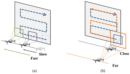
Figure 2.
Impact of UAV flight methods on the area photographed per unit of time: (a) UAV speed; (b) distance from the object.
In Figure 1, the optimal camera settings were identified for UAV flight methods of D = 3 m and v = 0.8 m/s, resulting in a minimum error of 2.1 mm. However, exploring alternative UAV flight methods under different D–v conditions, while maintaining the same area covered per unit of time, could potentially yield lower errors. This highlights the importance of examining various UAV flight methods under identical time constraints.
Figure 3 illustrates the optimization of UAV flight methods. In Figure 3a, the color assigned to each point on the D–v chart illustrates the minimum error achievable for each D–v condition at a given illuminance level (see Figure 1). For instance, a cyan color represents the minimum achievable error of 1.47 mm at D = 3 m, v = 0.3 m/s, and E = 100 lx. The optimal UAV flight method is determined by identifying the points with minimum RMSE values, which are marked as red dots in Figure 3b–e. These points are selected across all D–v conditions that correspond to equivalent A values, as indicated by the dashed lines in the figures.
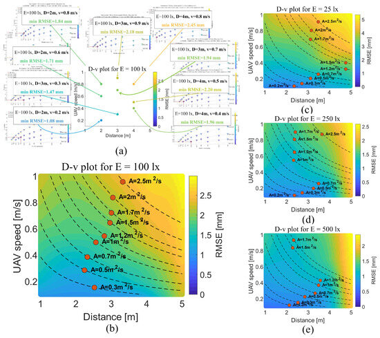
Figure 3.
Optimization of UAV flight methods under E–A constraints. (a) The procedure for generating a full D–v chart. (b) Optimization for E = 100 lx; each dashed line indicates points with identical A, with the red dot on each line indicating the point of minimum error for that specific A constraint. (c) Optimization for E = 25 lx. (d) Optimization for E = 250 lx. (e) Optimization for E = 500 lx.
The relationship between the optimal (D, v) and A is complex, as it is affected by variations in camera settings at each (D, v) point. In Figure 3b, the most favorable D–v condition for A = 0.5 m2/s, D = 2 m, and v = 0.3 m/s leads to a minimum error of 1.25 mm with camera settings of t = 1/100 s, N = 3.5, S = 3200, and p = 1920 px. In contrast, for A = 1.5 m2/s with D = 3 m and v = 0.7 m/s, the minimum error is 1.97 mm using camera settings of t = 1/160 s, N = 2.8, S = 3200, and p = 1920 px. Furthermore, the optimal (D, v) also varies depending on illuminance levels. For example, at E = 100 lx, the optimal UAV flight method for A = 0.5 m2/s is D = 2 m and v = 0.3 m/s (as shown in Figure 3b), whereas at E = 250 lx, it shifts to D = 3 m and v = 0.2 m/s for the same A (as shown in Figure 3d).
2.3. Step-by-Step Process of the OPS Determination
OPS is defined as the combination of the optimal camera settings and the optimal UAV flight methods that minimize error under given illumination and time constraints. The process of determining the OPS consists of four main steps (Figure 4): (1) Measure the illumination level (E) using a lux meter. In the absence of a lux meter, auto-exposure settings can serve as an alternative method to estimate relative brightness levels, although they may lack the absolute accuracy of dedicated illuminance sensors. (2) Calculate the required area to be photographed per unit of time (A); (3) determine the optimal UAV flight methods (D, v); (4) determine the optimal camera settings (N, t, S, p). While Steps 1 and 2 can be performed in any order, Step 3 requires the completion of both Steps 1 and 2, and Step 4 needs Steps 1, 2, and 3 to be completed beforehand. For a measured illuminance of 100 lx, with the requirement to photograph the entire target area of 100 m2 within 4 min, the OPS were identified as follows: flying a drone at D = 2 m with v = 0.3 m/s, combined with camera settings of N = 3.5, t = 1/100 s, S = 3200, and p = 1920 px.
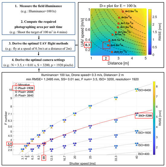
Figure 4.
Flow chart for deriving the OPS for UAV-based SfM–MVS.
A point of potential confusion is that the D–v chart, utilized in Step 3, is derived from analyzing the minimum camera setting values under various E–D–v conditions, as detailed in Step 4. Nevertheless, determining the optimal UAV flight methods must precede the selection of optimal camera settings, as the latter is influenced by the former. It is important to note that the optimal UAV flight methods identified in Step 3 are only effective when combined with the optimal camera settings identified in Step 4. This dependency highlights the intricate relationship between UAV flight methods and camera settings in minimizing error.
3. Application of the OPS
This section presents examples of OPS applications and evaluates their effectiveness. Point clouds generated employing the OPS were compared with those obtained employing arbitrary photography settings (APS). The APS were not chosen freely but were selected from camera settings that satisfy Equation (2) to ensure adequate image brightness, and from UAV flight methods that were constrained by the same time limitations (Equation (3)). Furthermore, the performance of SfM–MVS utilizing the OPS was compared to LiDAR data acquired from an underground tunnel construction site. This comparison aimed to demonstrate the potential of the OPS in enhancing the performance of SfM–MVS under challenging environmental conditions.
3.1. Comparison Between the OPS and APS Under Laboratory Conditions
An experimental setup was designed in a laboratory to evaluate the error differences between the OPS and APS. A textured reference target was established on a vertical flat wall consisting of three planes, each with 60 cm edge lengths and inclined approximately 27 degrees from the wall (Figure 5). Three LED lamps were placed to ensure uniform diffuse illumination across the target, and their intensity was adjustable to control illuminance levels.
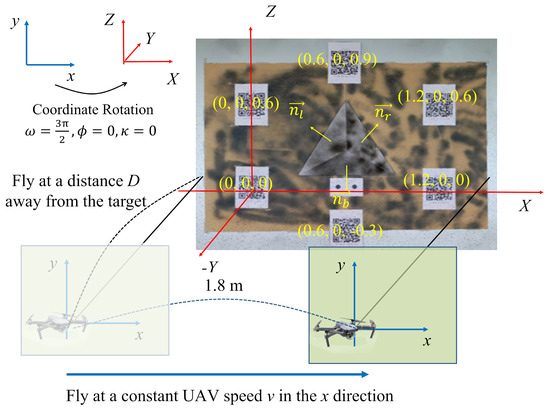
Figure 5.
Flow chart for deriving the OPS for UAV-based SfM–MVS. Experimental setup and axis settings. The normal vector for the left plane is represented as nl = (0.423, 0.876, −0.217), for the right plane as nr = (0.438, 0.869, −0.229), and for the bottom plane as nb = (−0.001, 0.857, 0.516). ω, ϕ, and κ represent the rotation angles around the x-, y-, and z-axes, respectively, between the 2D camera coordinate system and the 3D object coordinate system.
To minimize systematic errors, six QR codes were utilized as GCPs [8,39]. These QR codes were generated using the “ContextCapture Target Creator” feature within Bentley’s ContextCapture software (v10.17.0.39). This feature allows the creation of QR codes embedded with predefined 3D coordinates (x, y, z) in a local coordinate system, specified in meter units. In this study, the QR codes were arranged in a hexagonal layout (Figure 5), and their physical placement was performed using a ruler, ensuring an accuracy within 1 mm. When the images containing these QR codes were processed in ContextCapture, the software automatically recognized the center of each QR code as the predefined coordinates. The detected coordinates exhibited an RMS 3D error of 4.9 mm (ranging from 4.5 to 5.2 mm). This error was primarily attributed to limitations in ruler precision during placement and variations in GSD caused by differences in image resolution and camera distance.
The imagery was captured using a DJI Mavic 2 Pro drone camera, with the onboard gimbal helping to dampen vibrations. A parallel-axis image acquisition scheme was employed, ensuring the camera’s viewing angle remained consistently orthogonal to the target [7]. Instead of taking individual photographs, a video was recorded at 24 fps in a single take, and frames were later extracted from the video. During the video capture, the UAV maintained a constant horizontal flight speed, ensuring that the extracted frames were sequential with uniform baseline distances. To prevent systematic errors due to insufficient image overlap, 20 frames were selected [7,38], with the total distance from the center of the first frame to the center of the last frame measuring 1.8 m.
The experiment involved capturing the target using the OPS and two APS under specific constraints of illuminance (E = 100 lx) and a combined factor of distance and velocity (D × v = 1.8 m2/s), which, considering the FOV of the camera, corresponded to A ≅ 1.4 m2/s. Following the proposed methodology (Figure 4), the OPS were determined, and as previously mentioned, the APS were selected based on camera settings and UAV flight methods that satisfied these constraints. Details of these photography settings are provided in Table 2.
Table 2.
The photography settings utilized for the laboratory experiment. Each setting was repeated 5 times, resulting in a total of 15 shots.
For point cloud generation, Bentley’s ContextCapture software was utilized, and the camera calibration was fixed to specified values during the SfM–MVS procedure [16]. To avoid potential smoothing effects that could occur during 3D mesh production [45], the final outputs were produced in 3D point cloud format (LAS format) rather than 3D mesh models. The generated 3D point clouds were then registered to a predefined object coordinate system using the open-source 3D point-cloud processing software CloudCompare v2.12 alpha, ensuring that the data from different settings could be accurately compared and analyzed.
Due to the challenges in accurately identifying the reference point locations of distorted points [1], direct measurement of point-to-point errors is difficult. Instead, we measured the distances from the point cloud to the planes of the reference target (denoted as εplane), which are straightforward to measure, and converted these values to PP-type RMSE (εpoint). The conversion from εplane to εpoint is based on Equation (4) and can be applied when the reference target has a planar shape [30].
where dxk and dyk represent errors on the image plane, while r1 and r2 are the column vectors of the rotation matrix that converts 2D image coordinates to 3D object coordinates. Additionally, n denotes the normal vector of the reference target plane (Figure 5). The comparison results of εpoint for the OPS and two APS are presented in Section 4.1.1.
3.2. Comparison Between the OPS and APS Under Field Conditions
The effectiveness of the OPS was validated through a field experiment conducted at Mt. Gwanak, Seoul, Republic of Korea. The site features a well-exposed rock mass outcrop (Figure 6) composed of Jurassic-age granite bedrock. The joint planes, primarily oriented in the southeast and northeast directions, consist of smooth, planar surfaces characteristic of tensile fracturing. Additionally, previous studies utilizing LiDAR surveys at the same site have been reported [48].
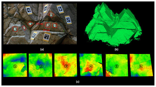
Figure 6.
(a) An image of the outcrop rock mass located at Mt. Gwanak, Seoul, Republic of Korea. (b) Reference model scanned with the SCANTECH KSCAN Magic laser scanner with a GSD of 1 mm. (c) Reference models of each joint plane, rescanned with a finer GSD of 0.1 mm. Joint planes are numbered from 1 to 6 for indexing purposes.
The site features a rock mass outcrop approximately 3 × 2.5 m in size. We designated six joint planes as targets, each measuring 15 × 15 cm, with their indices displayed in Figure 6. Instead of creating a separate 3D model for each joint plane, we surveyed the entire site and then extracted the six joint planes from the complete 3D model. The reference 3D model was captured using a high-precision handheld laser scanner, the SCANTECH KSCAN Magic (SCANTECH (HANGZHOU) CO., LTD., Hangzhou, China; Table 3), which offers an accuracy of 0.05 mm and a GSD of 0.05 mm. To ensure high accuracy, calibration markers were attached to the target surface, which partially obstructed some sections of the rock face. The entire site was first scanned with a GSD of 1 mm. Subsequently, only the region of interest—the six joint planes and their vicinities—was rescanned at a finer GSD of 0.1 mm to minimize the scanning time. However, despite the scanning area covering only 7.5 m2, the scanning process required seven hours, making it impractical for routine on-site surveys.
Table 3.
SCANTECH KSCAN-Magic laser scanner specification (https://www.3d-scantech.com/product/kscan-magic-composite-3d-scanner/, accessed on 2 March 2025).
For the SfM–MVS process, we attached six April codes uniformly around the target region and used them as GCPs to minimize systematic errors [8,39]. The distances between the April codes were measured and input into ContextCapture software, which automatically recognized the codes and provided absolute scale information. The target joint planes were captured under two different illuminance constraints (E = 50, 1500 lx) and one time constraint (A = 0.3 m2/s). These targets were located in an open-air environment, where illuminance was indirectly controlled by adjusting the time or weather conditions of the survey. For instance, 50 lx corresponds to low brightness and similar post-sunset conditions, while 1500 lx represents intermediate brightness, typical of a cloudy day. Brighter conditions, such as those on a sunny day, were deliberately avoided, as non-diffuse illumination (e.g., shadowed areas) could introduce systematic errors. The time constraint (A = 0.3 m2/s) reflects realistic conditions found in tunnel construction site surveys, where rock faces measuring 50–200 m2 must be surveyed within 3–10 min.
We used a camera mounted on the DJI Mavic 2 Pro drone and employed a parallel-axis image acquisition scheme. A single video was recorded per shot while the drone maintained a constant horizontal flight speed. For 50 lx, we captured four videos, with each OPS and one APS repeated twice. For 1500 lx, we recorded eight videos, repeating the OPS and three APS twice each. Details of these photography settings are provided in Table 4. From each video, 50–60 frames were extracted and processed using ContextCapture software to generate 3D point clouds of the rock mass.
Table 4.
The photography settings utilized for the outcrop rock mass survey include settings #1 and #3 as the OPS, and the other settings as the APS. Each setting was repeated twice, resulting in a total of 12 shots.
The error correction method used for the indoor target (detailed in Equation (4)) was feasible because the target consisted of flat planes. However, this method could not be applied to the non-flat geometry of the target joint planes. Consequently, alternative quantitative indicators relevant to error assessment were measured [49]: The cloud-to-mesh (C2M) distance and the multiscale model-to-model cloud comparison (M3C2) distance [50]. In this study, point clouds generated using SfM–MVS were compared against a reference 3D model produced by laser scanning. The standard deviation (std) of the C2M and M3C2 distances (stdC2M and stdM3C2, respectively) served as the quality indicator for the point clouds, with calculations performed using CloudCompare software (Figure 7). Approximately 30 visually corresponding feature points between the reference model and the point clouds were identified initially. The models were then coarsely aligned based on these feature points, followed by a more precise alignment using the iterative closest point (ICP) algorithm. From the 3D models, we extracted six joint planes, each measuring 15 × 15 cm. The “compute cloud/mesh distance” function in the software was used to calculate the stdC2M for each joint plane under each photography setting (Figure 7d,e). Similarly, the “M3C2 distance” function in the software was used to calculate the stdM3C2 with the default parameter settings utilized. The comparison results for the stdC2M and stdM3C2 between the OPS and APS are presented in Section 4.1.2.
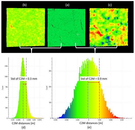
Figure 7.
Example of calculating the stdC2M distances. Colors represent the C2M distances to the reference model. The same procedure was conducted for calculating the stdM3C2 distances: (a) Reference model of joint plane #2; (b) point cloud generated using SfM–MVS with settings #3; (c) point cloud generated using SfM–MVS with settings #4; (d) histogram of C2M distances for settings #3, with a resulting stdC2M of 0.3 mm; (e) histogram of C2M distances for settings #4, with a resulting stdC2M of 0.9 mm.
3.3. Comparison with LiDAR Data
Underground tunnel construction sites feature a low-light environment, and the surveying time is often limited due to ongoing construction activities. Moreover, the Global Navigation Satellite System (GNSS) is typically unavailable in tunnels, further complicating the surveying process. To evaluate the SfM–MVS method under such challenging conditions, we implemented SfM–MVS using the OPS and conducted a comparative analysis with LiDAR. This comparison was conducted at an underground tunnel construction site in Yeoju-si, Republic of Korea, where a surveying team used a LiDAR instrument to scan the tunnel face. As shown in Figure 8, the target rock face area was approximately 70 m2. With the help of field lighting (Figure 8a), the illuminance in the area was approximately 25 lx.
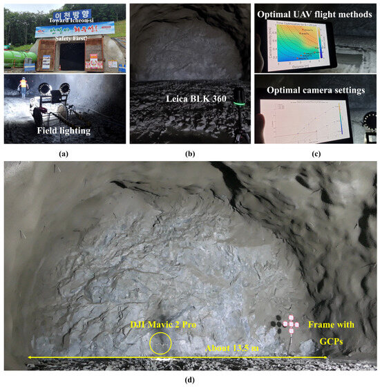
Figure 8.
Field application of SfM–MVS using the OPS at an underground tunnel construction site in Yeoju-si, Republic of Korea: (a) Entrance of the tunnel and field lighting inside; (b) the Leica BLK 360 LiDAR used by the site surveying team; (c) derivation of the OPS for the site; (d) the target rock face and DJI Mavic 2 Pro used in the survey. A frame with GCPs was placed in front of the tunnel face.
The surveying team utilized a Leica BLK360 imaging laser scanner (Leica Geosystems AG, Heerbrugg, Switzerland; Figure 8b), with its specifications detailed in Table 5. It is important to distinguish between the ranging accuracy, which refers to errors in the direction of the laser beam, and 3D point accuracy. The error term in this study corresponds specifically to the 3D point accuracy listed in Table 5. The LiDAR instrument was positioned 10 m away from the tunnel face, and the scanning process took approximately 5 min, which is a typical duration for surveying in tunnel construction sites. The laser-scanned data were then post-processed using Leica Cyclone REGISTER 360 software v2022.1.0 to remove outlier points and refine the dataset.
Table 5.
Leica BLK360 imaging laser scanner specifications (https://leica-geosystems.com/products/laser-scanners/scanners/blk360 accessed on 2 March 2025).
Since the field survey team operated the LiDAR instrument for 5 min, the required time constraint was calculated as A = 70 m2/4 min, allowing for a tolerance period to accommodate the approach and retreat of the drone. Under the constraints of E = 25 lx and A = 0.3 m2/s, the OPS were determined as follows (Figure 8c): N = 2.8, t = 1/40 s, S = 3200, p = 1920 px, D = 3 m, and v = 0.2 m/s. The overall shooting method remained consistent with the previous sections. However, one notable difference from the previous sections was the deployment and distribution of GCPs. Although it was not feasible to place GCPs evenly along the tunnel face due to safety concerns and restricted accessibility, an independent frame was positioned in front of the tunnel face, equipped with five GCP QR codes (Figure 8d). These QR-coded GCPs were utilized to scale the reconstructed models and minimize systematic errors.
Additionally, the DJI Mavic 2 Pro drone camera could not capture the entire height from the floor to the ceiling (approximately 6.4 m) within its FOV when positioned 3 m away. As a result, the drone had to fly a zig-zag path (refer to Figure 2), which required acceleration and deceleration at both ends. Nonetheless, the majority of the shooting was conducted at a uniform drone speed, and only the frames captured during this uniform flight speed were utilized for analysis.
Unlike the validation described in Section 3.1 or Section 3.2, obtaining a reference model for the tunnel face was not feasible due to time limitations. Instead, we compared the point clouds generated by both methods using quantitative indices such as point resolution and idealistic accuracy, and qualitative indices like joint expression capability. The results of these comparisons are presented in Section 4.2.
4. Results
Section 2 outlined the procedure for deriving the OPS under illuminance and time constraints. To highlight the importance of the OPS, we compared the quality of point clouds obtained using the OPS with those obtained using the APS (Section 3.1), with detailed results presented in Section 4.1. Furthermore, to demonstrate the potential of the SfM–MVS method when utilizing the OPS, we conducted a comparative analysis of point cloud quality between SfM–MVS and LiDAR in an underground tunnel site (Section 3.2), where both lighting conditions and surveying time were limited. The results of this comparison are detailed in Section 4.2.
4.1. Effectiveness of the OPS
In Section 3.1, we evaluated the effectiveness of the OPS by comparing the quality of the point clouds obtained using the OPS and APS. First, the error levels in the point cloud of an indoor reference target, which consisted of flat planes, were assessed, and then the stdC2M distances for the joint planes on a rock mass outcrop in Mt. Gwanak were compared.
4.1.1. Point Cloud Errors for the Indoor Reference Target
We generated 3D point clouds of an indoor reference target using the OPS and two APS under E = 100 lx and A = 1.4 m2/s, with five repetitions for each setting. The camera orientation and lens correction parameters were well calibrated, resulting in an average reprojection error of less than 1 px during the SfM procedure [39]—OPS = 0.67–0.7 px, APS#1 = 0.68–0.69 px, and APS#2 = 0.65–0.66 px.
Figure 9 illustrates the point cloud error levels for the reference. A significant difference in error levels was observed between the OPS and APS. The mean error level for the OPS (red dots in Figure 9) was 2.59 mm, while the APS results showed notably higher errors: 7.58 mm for APS#1 (cyan squares in Figure 9) and 8.67 mm for APS#2 (green diamonds in Figure 9). The improvement in error levels when using the OPS was expected, as it represents the minimum error achievable with photography settings derived from the error pre-determination model developed by Leem et al. [30], which has demonstrated high predictive performance (note the alignment between the predicted and observed RMSEs in Figure 9). Furthermore, severe distortion in the representation of flat planes was observed in the APS-generated point clouds, as shown in the side views of Figure 9. Notably, without modifying the existing illuminance and time constraints, substantially better point cloud quality could be achieved simply by adjusting the camera settings and UAV flight methods.
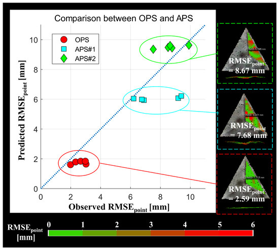
Figure 9.
Comparison between the OPS and APS under E = 100 lx and A = 1.4 m2/s (D × v = 1.8 m2/s) constraints. The side views on the right are vertically exaggerated to help the reader’s understanding.
4.1.2. StdC2M Distances for the Joint Planes on an Outdoor Rock Mass
We generated 3D models of an outdoor rock mass using both laser scanning and SfM–MVS. The laser-scanned model served as the reference, and we measured the stdC2M and the stdM3C2 between the reference model and those generated using SfM–MVS. In total, 12 shots were taken, including four for the OPS and eight for the APS. Additionally, the camera orientation and lens correction parameters for the SfM–MVS were well calibrated, with reprojection errors ranging from a minimum of 0.43 px to a maximum of 0.67 px. Since the mean values of C2M or M3C2 were significantly lower than the std values (maximum mean of C2M: 0.038 mm, minimum stdC2M: 3.01 mm; maximum mean of M3C2: 0.057 mm, minimum stdM3C2: 3.04 mm), it can be inferred that the SfM–MVS-generated models were well registered with the reference model.
The stdC2M and stdM3C2 values of the OPS and APS are listed in Table 6 and Table 7, respectively, with their comparison illustrated in Figure 10. In the figure, red dots represent the std values for the OPS, while black dots indicate the std values for the APS. It is evident that the red dots consistently lie below the black dots under both 50 and 1500 lx conditions. With the exception of two cases for stdC2M (joint planes #4 and #5, E = 1500 lx), where the APS achieved the second lowest stdC2M, the lowest and second lowest stdC2M and stdM3C2 values were obtained using the OPS in all other cases. This result suggests that the OPS can generate 3D models that more closely resemble the reference than those created using the APS, thereby indicating that the OPS produced more accurate 3D models.
Table 6.
StdC2M for each photography setting across joint planes #1 to #6, listed in millimeter units. The lowest and second-lowest stdC2M values for each plane are highlighted in bold.
Table 7.
StdM3C2 for each photography setting across joint planes #1 to #6, listed in millimeter units. The lowest and second-lowest stdM3C2 values for each plane are highlighted in bold.
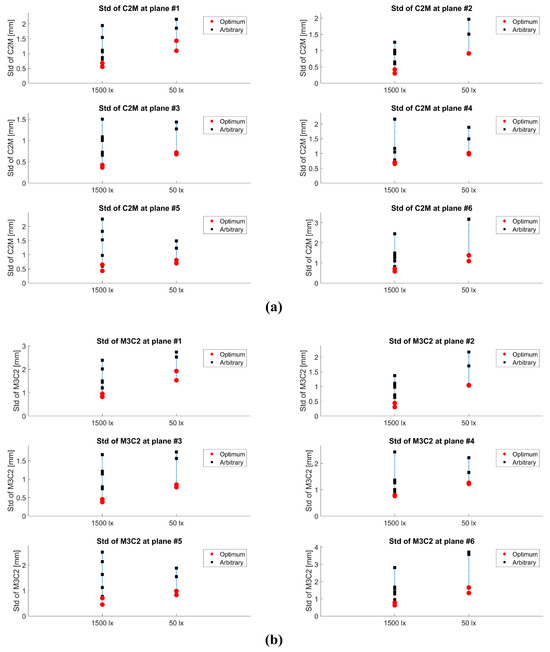
Figure 10.
Comparison of std values for joint planes #1 to #6. Red dots represent the std values for the OPS, and black dots represent the std values for the APS: (a) StdC2M comparison; (b) stdM3C2 comparison.
4.2. The Potential of SfM–MVS Utilizing OPS for Enhanced 3D Modeling
In Section 3.3, we generated the point cloud of an underground tunnel rock face using both SfM–MVS with OPS and LiDAR. During the SfM process, the reprojection error was measured at 0.54 px, confirming the calibration accuracy. Although the OPS were determined with a time constraint of 4 min, allowing for drone approach and retreat as well as acceleration and deceleration phases, the actual shooting time was extended to 5 min, matching the duration required for LiDAR operations.
The LiDAR-generated point cloud is displayed in Figure 11a. The surveying team operated the LiDAR instrument to collect data over a 360-degree range, capturing a total of 12,100,000 points. However, the point resolution for the tunnel face was relatively low, at approximately 1,700,000 points, equivalent to 150 pts/m2. This lower point density resulted from the chosen scanning approach, where the surveying team conducted a full 360-degree scan instead of restricting data collection to the tunnel face. Although the instrument is capable of achieving higher resolutions, the limited shooting time of 5 min constrained the resolution of the LiDAR-generated point cloud, as LiDAR collects discrete point samples rather than capturing continuous surface data [51]. As a result of the active nature of laser scanning [51], intensity data were captured, offering some insights into the surface characteristics. However, this method was ineffective in capturing the texture of the rock mass, even though texture is a crucial factor in rock characterization. According to its specifications (Table 5), the LiDAR method would have resulted in a point cloud error of 6 mm when measured from a distance of 10 m. While higher-end LiDAR units could achieve greater point density and accuracy within the same time frame, this would come at the cost of higher equipment expenses.
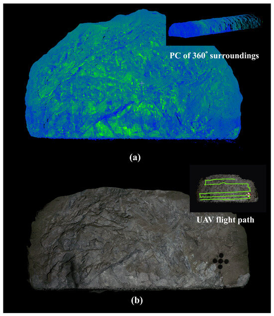
Figure 11.
Point clouds generated by LiDAR and SfM–MVS with OPS: (a) point cloud generated by LiDAR; (b) point cloud generated by SfM–MVS utilizing OPS. The image acquisition trajectories (UAV flight path) are illustrated in the upper right section.
SfM–MVS generated a high-resolution point cloud of the tunnel face, containing approximately 35,100,000 points (670 pts/m), which increased to 39,700,000 points when including the surrounding area. This resolution is approximately 20 times higher than that achieved by LiDAR, as illustrated in Figure 11b. The significant contrast in point counts mainly stems from whether the instrument only targets the tunnel face. When considering the total number of points generated, the difference narrows to approximately 3.3 times. Although additional time is required to generate 3D point clouds, the duration varies based on computational power, resolution, and the number of images used. Since LiDAR data also require post-processing, our focus was on the potential to generate high-resolution 3D models within the allocated field shooting time. Since SfM–MVS is based on photographic images, it effectively captures the texture of the rock mass, though it lacks the ability to obtain intensity data like LiDAR. The passive nature of photographic images allows SfM–MVS to achieve high-resolution data over a broad area within a short shooting period [51]. When utilizing OPS, the SfM–MVS method would likely result in a point cloud error of 2 mm under the constraints of E = 100 lx and A = 0.3 m2/s (refer to Section 2.1).
In addition to quantitative indices, we qualitatively compared the point clouds from both methods. Given that the target area was a tunnel construction site, we focused on the capability of each method to express joint planes and joint traces, which are critical for rock mass stability analysis. Figure 12a presents the comparison of joint plane expression capabilities. Both methods successfully depicted the normal vectors of joint planes within a five-degree deviation, which is better than typical human bias. However, both methods exhibited point resolutions lower than the commonly referenced laboratory values of 1000 pts/m [52] to 10,000 pts/m [53] used for measuring surface roughness. However, due to its lower resolution, LiDAR had more significant issues with underestimating the joint roughness compared to SfM–MVS [54].
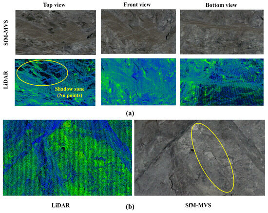
Figure 12.
Comparison of rock mass characterization capabilities between SfM–MVS and LiDAR: (a) joint plane expression capabilities; (b) joint trace expression capabilities.
Shadow zones (yellow ellipse in Figure 12a), areas where no points are recorded, appeared in the LiDAR data due to the use of a terrestrial laser scanner (TLS). Since TLS emits light from a fixed position, the light often fails to reach areas obscured from its direct line of sight, resulting in shadow zones. These absences of points can complicate the recognition of joint planes and their orientations during data analysis. In contrast, dark regions appeared in the SfM–MVS point cloud; however, unlike in LiDAR data, dark-colored points were recorded in these areas. This difference arises because SfM–MVS captures images from multiple viewpoints. While these dark-colored points may be subject to potential systematic errors due to low saturation, they still provide useful information for detecting plane existence and determining orientation. It is important to note that the dark regions in the SfM–MVS data are not equivalent to the shadow zones found in LiDAR data. While LiDAR combined with UAV technology (ULS) may mitigate shadow zone issues, it introduces other problems, including reduced accuracy and resolution, particularly in GNSS-denied environments [1].
Figure 12b presents a comparison of the joint trace expression capabilities. Joint traces vary in aperture from sub-millimeter to several millimeters. While LiDAR produced a point cloud that was overly sparse to effectively depict the joint traces, SfM–MVS was able to represent them up to 2 mm. Beyond resolution, the texture data captured by SfM–MVS proved advantageous in depicting joint traces, which appeared as dark-colored points (yellow ellipse in Figure 12b). The overall performance comparison between the two methods is summarized in Table 8.
Table 8.
Performance comparison between SfM-MVS utilizing the OPS and LiDAR at the Yeoju-si tunnel site.
5. Discussion
Although the quality of input images in the SfM–MVS procedure significantly influences the resulting 3D model accuracy, limited research has been conducted on optimizing both camera settings and UAV flight methods in an integrated manner. In contrast, this study introduced a simultaneous multi-parameter optimization framework that jointly considers the effects of camera settings, flight methods, and environmental conditions (i.e., illumination and time) on reconstruction accuracy. By systematically analyzing the influence of each contributing factor on reconstruction error, the proposed method identifies an optimal combination of photography settings that minimizes overall error, resulting in a globally optimal configuration.
5.1. Robustness of the OPS Derivation Procedure
In this study, we introduced a procedure to determine the OPS under illuminance and time constraints and validated its significance through a comparison with APS and LiDAR. Nonetheless, practical limitations may sometimes prevent the application of the derived OPS due to the limited availability of several factors such as UAV speed, distance, shutter speed, or resolution. For example, UAV speed and distance may be constrained by speed regulations, physical performance limitations, or altitude restrictions. These factors then act as upper or lower bounds for UAV speed and distance. Despite these constraints, a sub-optimal D–v combination can still be determined within the restricted D–v zone, as long as this feasible D–v combination meets the required A. For instance, if the minimum v is restricted to 0.6 m/s, one cannot use the optimal UAV flight method of v = 0.5 m/s and D = 2.5 m when A = 1 m2/s is required, as shown in Figure 3. In such cases, an alternative approach could be to adopt the second-best UAV flight method, which might involve approximately v = 0.6 m/s and D = 2 m, though this may result in a slightly higher error.
However, this represents an ideal scenario, and in practice, it is necessary to introduce the concept of a safety factor. For instance, drone battery performance can significantly influence UAV flight methods. Battery efficiency is closely linked to UAV speed, and in the case of large-scale sites, battery replacement must also be considered when designing an optimal flight strategy. Quantifying battery efficiency is challenging due to its strong dependency on hardware specifications and external environmental factors such as temperature and wind. Since the primary objective of this study was to propose a practical optimization strategy for UAV-based 3D reconstruction, battery performance considerations were not included in the optimization framework. Nevertheless, to ensure more stable flights and reliable image acquisition, particularly for large-scale surveys, future studies should explore the integration of a safety factor into the optimization of camera settings and UAV flight paths.
Occasionally, images captured under certain conditions may exhibit periodic noise, particularly under artificial lighting such as the LED strobe lights commonly used in underground mines or tunnels. This phenomenon often occurs when the camera’s rolling shutter fails to synchronize with oscillating light sources. Although the negative effects of periodic noise were not specifically evaluated in this study, they can be mitigated by adjusting the photography settings. If images captured using the OPS display periodic noise, users can attempt alternative settings with varying shutter speeds to eliminate the noise, albeit with a potentially higher error margin. For example, if the optimal camera settings shown in Figure 1 result in periodic noise, alternative settings like N = 3.2, t = 1/120 s, and S = 3200 or N = 2.8, t = 1/80 s, and S = 1600 can be tested. If these adjustments do not display periodic noise, they can be adopted despite the slightly increased error. If not, further adjustments should be explored until the issue is resolved.
The resolution of the resultant point cloud is crucial for analyses such as surface roughness measurements. For instance, a resolution ranging from 1000 pts/m [52] to 10,000 pts/m [53] is typically required to accurately measure the surface roughness in laboratory settings. The maximum resolution of a point cloud is achieved at the ideal GSD, which involves deriving a point from each image pixel. Thus, the sampling distance of the resultant point cloud, in meter units, is approximately (D × d)/(f × p), where d and f are generally fixed. Therefore, the resolution is primarily influenced by D and p.
Figure 13 illustrates the change in OPS when an additional GSD constraint is considered. Under E = 100 lx, D = 5 m, and v = 0.2 m/s, the optimal camera settings without the GSD constraint are t = 1/80 s, N = 2.8, S = 1600, and p = 1920, which achieve an ideal GSD of 3.3 mm and a minimum error of 2.3 mm (Figure 13a). When GSD is set to be less than 2 mm, settings that do not meet this requirement—including the previously optimal settings—are excluded (Figure 13c). The new alternative optimal camera settings in this case are t = 1/40 s, N = 2.8, S = 800, and p = 3840, resulting in a slightly higher minimum error of 2.5 mm. Considering that the resolution constraint increases the minimum achievable error, the revised settings still minimize the error while satisfying the resolution requirement. With these new E–D–v charts (note Figure 3a), it is possible to complete the new D–v chart for UAV flight method optimization (Figure 13d). It shows that regions with relatively far distances (D ≥ 4 m) are strongly affected by the GSD constraint (compare Figure 13b,d), which significantly impacts the selection of optimal UAV flight methods, particularly in higher A values.
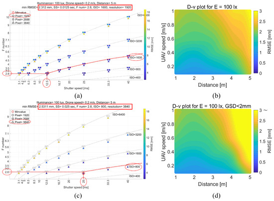
Figure 13.
Comparison of the OPS considering the GSD constraint: (a) the E–D–v chart under E = 100 lx, v = 0.2 m/s, and D = 5 m; (b) the D–v chart for E = 100 lx, identical to Figure 3b; (c) the new E–D–v chart with a GSD constraint of 2 mm; (d) the new D–v chart for E = 100 lx, reflecting the GSD constraint.
We introduced a procedure for determining the OPS for UAV-based SfM–MVS with parallel image acquisition. However, establishing the OPS for still imaging is beyond the scope of this study, as convergent acquisition schemes may offer better accuracy for still images [7]. Additionally, when considering time constraints, it is important to account for the acceleration or deceleration between still photography locations, which can vary significantly based on the physical performance of the camera platform. Nonetheless, since motion blur is not a concern in still images, a slower shutter speed can be used. This allows for a higher SNR in the image, making the prevention of out-of-focus blur the top priority. Therefore, we recommend setting the highest possible F-number, then the lowest ISO, and finally the slowest shutter speed that still maintains appropriate image brightness (Equation (2)).
This study assumed uniform photography settings across the entire image set. Consequently, the performance of the OPS might be compromised when using mixed image sets to generate a point cloud. For instance, if the target area includes both brightly and darkly illuminated areas, such as shadows, a separate OPS would be required for each lighting condition. This would result in a transition zone where images used for 3D reconstruction are captured with different settings. The performance in this transition zone could be diminished due to the inconsistent distortions across image sets. A study on orthophotos by Aasen et al. [3] noted that details in overlapping images tend to blend, rather than selecting the best details from each. Similarly, we anticipate that errors in the transition zone may average between the errors observed in the brightly and darkly lit regions.
Another challenge is when the surveyed area exhibits significant terrain variation, making it difficult to maintain a uniform distance from the target. In such cases, it is challenging to clearly define the distance to the target, or multiple distances may coexist. Similar to the transition zone observed under mixed lighting conditions, it becomes impossible to optimize the photography settings using a single OPS. A practical solution to overcome this is to increase the minimum distance for the OPS analysis area, setting it significantly larger than the terrain variation (sub-optimal OPS selection), where the impact of height differences can be neglected. However, identifying a minimum distance that sufficiently mitigates the effects of terrain variation requires further research.
UAV-based image acquisition inherently involves minor vibrations during flight, and although gimbals are employed to stabilize the camera, complete elimination of vibrational motion is not achievable. At higher flight speeds, motion blur typically dominates image degradation, rendering vibration-induced blur largely negligible. However, when UAVs operate at sufficiently low speeds, vibration blur becomes significant. This introduces a trade-off in flight speed selection: reducing speed to improve image sharpness inadvertently increases susceptibility to vibration-induced distortions. The magnitude of the vibration blur is influenced by various factors, including drone hardware specifications, environmental conditions (e.g., wind), and the effectiveness of internal damping mechanisms. Due to the stochastic nature of these factors, quantifying vibration blur is challenging. Since the objective of this study was to propose a practical optimization scheme for photographic settings, vibration blur was not explicitly considered in this study. Nevertheless, for more robust image acquisition strategies—particularly in low-speed UAV operations where vibration effects are more pronounced—future research should explore integrating vibration effects into the optimization of photography settings.
5.2. Sensitivity of the OPS
In Section 4, we demonstrated the effectiveness and potential of the OPS. When the SfM–MVS utilized the OPS, it achieved significant improvements in point cloud quality compared to the APS, without requiring additional lighting or extra time. However, it is crucial to use the optimal camera settings in conjunction with the optimal UAV flight methods, as the lowest error is achieved only when both are applied together. If only partial settings are implemented, such as using only the optimal UAV flight method while selecting camera settings arbitrarily, the combination is no longer optimal, and alternative settings may produce better results. Since camera settings are less likely to be adjusted during image acquisition, it is essential to meticulously maintain the UAV flight method through precise UAV path programming to preserve the effectiveness of the OPS.
In Figure 14, we demonstrate the variation in optimal camera settings based on UAV speeds (0.1, 0.5, and 0.9 m/s) and distances (1–9 m) under specific illuminance levels (600, 770, 970, and 1550 lx). The figure illustrates trends in camera settings adjustments according to UAV flight methods (D, v). Along the lines representing constant UAV speeds (colored red, green, and blue in Figure 14), one trend observed is the decrease in the F-number at larger distances. As the distance increases, motion blur in the image decreases, shifting the priority to reducing out-of-focus blur by lowering the F-number. Another trend is the need for faster shutter speeds at higher UAV speeds for the same distance, moving from red to green and then from green to blue in Figure 14. This adjustment is necessary to reduce motion blur, thus taking precedence over reducing the F-number at higher UAV speeds. Once the maximum aperture (or minimum F-number) is reached, using a slower shutter speed becomes the only option. Importantly, the selection of optimal camera settings is more critical at close distances and slow UAV speeds and becomes less sensitive at greater distances and faster UAV speeds. Therefore, precise maintenance of the UAV flight method is crucial when operating under short time constraints.
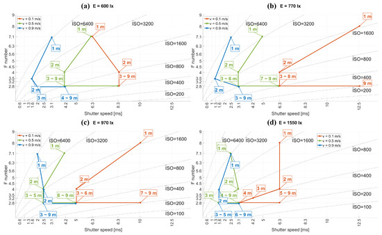
Figure 14.
The sensitivity of selecting optimal camera settings for UAVs varies with changes in speed (0.1, 0.5, and 0.9 m/s), distance (1–9 m), and illuminance (600, 770, 970, and 1550 lx). Subfigures (a–d) correspond to illuminance levels of 600, 770, 970, and 1550 lx, respectively. Each point on the chart represents the optimal camera settings under specific E–D–v conditions.
The variation in optimal camera settings also correlates with illumination, though no clear relationship between reducing the F-number and using faster shutter speeds is evident when illumination changes. However, a consistent trend is observed in the camera settings moving toward the lower left of the charts from Figure 14a–d, despite varying illuminance intervals (ΔE = 170, 200, and 480 lx). For instance, at D = 1 m and v = 0.5 m/s (top points on the green lines), the F-number (N) decreased from 6.3 to 5 (a reduction to 0.8 times the original) when the illumination increased from 600 to 770 lx (ΔE = 170 lx; from Figure 14a,b). Meanwhile, N decreased from 4.2 to 2.5 (a reduction of 0.6 times the original) when the illumination jumped from 970 to 1550 lx (ΔE = 480 lx; from Figure 14c,d). Despite the near tripling in illuminance change, the alteration in camera settings was relatively minor. This indicates that the selection of optimal camera settings is particularly sensitive under low illumination conditions, similar to the sensitivity observed under limited time constraints. The balance between error minimization and sensitivity under varying conditions warrants further investigation. Consequently, extra caution is advised when employing the OPS under low illuminance and short time constraints.
Concerns have been raised about the sufficiency of SfM–MVS-generated point clouds in underground tunnels, where limited lighting and constrained surveying time might distort the captured images [29]. Traditionally, LiDAR has been used for 3D rock mass modeling in such underground spaces, despite its high capital costs, issues with shadow zones, lack of texture detail, and lengthy surveying times. However, when SfM–MVS is utilized with OPS, it shows potential for more effectively characterizing underground rock masses by generating high-quality 3D point clouds at a lower cost (refer to Table 8). Previous studies [1,6,7] have noted the superior performance of SfM–MVS compared to LiDAR, and our findings reinforce this advantage in challenging environments characterized by low lighting and limited time. The purpose of this study was not to claim the outright superiority of SfM–MVS over LiDAR but to demonstrate that SfM–MVS can achieve sufficient performance even in challenging environments. As discussed, each method has its own advantages and limitations, and they should ideally be used in a complementary manner.
Certain challenges may arise when applying UAV-derived SfM–MVS in underground spaces. For instance, a single UAV may not satisfy the time constraints due to ongoing construction activities. Operating multiple UAVs simultaneously could be a viable solution, as the cost of moderate UAVs is relatively low compared to LiDAR and other laser scanning methods. Similarly, the accuracy of the resultant point cloud could be improved with the use of multiple UAVs. For example, as shown in Figure 3, using a single UAV under a time constraint of A = 1 m2/s might achieve a minimum error of approximately 1.7 mm. However, by deploying two UAVs simultaneously, where each UAV covers half of the target area and operates under a time constraint of A = 0.5 m2/s, the minimum error could be reduced to approximately 1.2 mm.
Excessively low illuminance conditions in underground tunnels pose a significant challenge. In such cases, no camera settings may achieve adequate image brightness (Equation (2)), and the impact of read or dark current noise becomes more pronounced. Addressing this lack of light with field lighting alone may not be feasible, as it is difficult to increase the illumination across an entire rock face in an underground tunnel. A more practical solution might involve equipping UAVs with their own lighting sources to illuminate the specific areas being photographed. However, to avoid systematic errors, the lighting must be homogeneous across the scene and capable of covering a larger area than the camera’s FOV. Furthermore, the distance from the target affects the illumination intensity, influencing the selection of OPS. Future research should explore this relationship further and its impact on determining OPS.
6. Conclusions
Based on the error prediction model developed in our previous work [30], we identified the optimal photography settings that minimize error under specific illuminance and time constraints. The efficacy of the OPS was validated by comparing the point cloud quality obtained from both an indoor reference target and an outdoor rock mass, using optimal versus arbitrary photography settings. The use of OPS enabled the generation of higher-quality point clouds without requiring increased illumination or additional surveying time.
Furthermore, we demonstrated the potential of SfM–MVS, utilizing the OPS, at an underground tunnel construction site by comparing its performance with the LiDAR method. Given the low illuminance and limited surveying time typical of such environments, which are generally challenging for photography, SfM–MVS with the OPS showed the potential to be more effective than LiDAR, offering higher accuracy and resolution at a lower cost.
Author Contributions
Conceptualization, J.L.; methodology, J.L.; validation, J.L., S.M. and I.-S.K.; investigation, J.L. and D.-H.Y.; resources, I.-S.K. and D.-H.Y.; writing—original draft preparation, J.L., S.M., I.-S.K., Y.S. and J.J.; visualization, J.L. and S.M.; supervision, J.-J.S. and J.J.; project administration, J.-J.S.; funding acquisition, J.-J.S.; software, J.L. and S.M. All authors have read and agreed to the published version of the manuscript.
Funding
This research was supported by the Energy & Mineral Resources Development Association of Korea (EMRD) funded by the Korea government (MOTIE) (grant no. 2021060003, Training Program for Specialists in Smart Mining), and by the Korea Institute of Energy Technology Evaluation and Planning (KETEP) grant funded by the Korea government (MOTIE) (grant no. 20214000000500, Training program of CCUS for the green growth).
Data Availability Statement
The data that support the findings of this study are available from the author, J. L., upon reasonable request. A derivation of OPS has been developed as an app and can be accessed at the following repository: https://github.com/sooyalim/Optimal-Photographing-Settings-OPS-, accessed on 2 March 2025.
Conflicts of Interest
The authors declare no conflicts of interest.
Abbreviations and Symbols
The following abbreviations and symbols are used in this manuscript:
| Abbreviations | |
| SfM | Structure from motion |
| MVS | Multiview stereo |
| LiDAR | Light Detection and Ranging |
| DEM | Digital elevation model |
| UAV | Unmanned aerial vehicle |
| PP | Point-to-point |
| PR | Point-to-raster |
| RR | Raster-to-raster |
| TS | Total station |
| dGPS | Differential global positioning system |
| RMSE | Root mean squared error |
| ME | Mean error |
| MAE | Mean absolute error |
| OPS | Optimal photography settings |
| APS | Arbitrary photography settings |
| ISO | International Organization for Standardization |
| SNR | Signal-to-noise ratio |
| BA | Bundle adjustment |
| GCP | Ground control point |
| FOV | Field of view |
| GSD | Ground sampling distance |
| C2M | Cloud-to-mesh |
| M3C2 | Multiscale model-to-model cloud comparison |
| stdC2M | Standard deviation of the C2M distances |
| stdM3C2 | Standard deviation of the M3C2 distances |
| ICP | Iterative closest point |
| GNSS | Global Navigation Satellite System |
| Symbols | |
| t | Camera shutter speed |
| N | Camera F-number |
| S | Camera ISO value |
| p | Camera pixel resolution |
| D | Distance from the target |
| v | UAV or camera platform speed |
| d | Camera sensor size |
| f | Camera focal length |
| ε3D | Errors in SfM–MVS-generated point clouds |
| ε2D | Image errors |
| εplane | Point-to-plane-type RMSE |
| εpoint | Point-to-point-type RMSE, equivalent to ε3D |
| s | Scaling factor |
| E | Illumination |
| M | Maximum template size |
| Q | Nosie sensitivity coefficient |
| A | Area photographed per unit of time |
Appendix A
This section provides a brief summary of the theoretical background for the error predetermination for each photography setting [30]. Equation (1) suggests that the error present in the image is propagated to the resulting point cloud, where it is amplified by the scaling factor s. The error within the pixel domain of the image can be quantified using Equation (A1) [30].
where the indices i and j represent the pixel coordinates within an image and P((i,j)∣(x,y)) denotes the probability that a point (x,y), where x and y are within the range [−0.5,0.5], is expected to be observed at the pixel location (0,0) but is instead observed at a different pixel location (i,j) due to distortion effects. This probability is determined by the extent of distortion within the pixel domain, represented by Δx and Δy, which arise from various sources such as motion blur, out-of-focus blur, and noise.
The magnitude of motion blur, denoted as B, is determined using Equation (A2), while the distortion effects caused by motion blur, represented by Δxmb and Δymb, are calculated using Equation (A3) [30].
where d stands for the sensor size, U denotes a uniform probability density distribution, and Trap refers to a trapezoidal-shaped probability density distribution. The influence of the maximum template size M utilized in the MVS algorithm was analyzed by Leem et al. [30], highlighting its role in mitigating the motion blur distortion when B exceeds M.
The level of out-of-focus blur, represented by σob, is determined using Equation (A4), while the distortion effects resulting from out-of-focus blur, denoted as Δxob and Δyob, are calculated using Equation (A5) [30].
where the notation N stands for a normal probability density distribution, and H denotes the focus distance, which, for this work, was set to the hyperfocal distance. This setting ensures that the camera maintains sharp focus from the hyperfocal distance to infinity, optimizing the depth of field for the broadest range of clear vision.
The noise-to-signal ratio or the reciprocal of SNR (signal-to-noise ratio), represented by σn, is derived from Equation (A6), while the distortion effects caused by noise, denoted as Δxn and Δyn, are calculated using Equation (A7) [30].
where E stands for the level of illumination and Q denotes the noise sensitivity coefficient, which varies with the type of camera used. The probability P((i,j)∣(x,y)) can then be determined through Monte Carlo simulations, incorporating the distortion effects caused by motion blur (Equation (A3)), out-of-focus blur (Equation (A5)), and noise (Equation (A7)).
References
- Smith, M.W.; Carrivick, J.L.; Quincey, D.J. Structure from motion photogrammetry in physical geography. Prog. Phys. Geogr. 2016, 40, 247–275. [Google Scholar] [CrossRef]
- Kovanič, Ľ.; Peťovský, P.; Topitzer, B.; Blišťan, P. Spatial Analysis of Point Clouds Obtained by SfM Photogrammetry and the TLS Method—Study in Quarry Environment. Land 2024, 13, 614. [Google Scholar] [CrossRef]
- Aasen, H.; Burkart, A.; Bolten, A.; Bareth, G. Generating 3D hyperspectral information with lightweight UAV snapshot cameras for vegetation monitoring: From camera calibration to quality assurance. ISPRS J. Photogramm. Remote Sens. 2015, 108, 245–259. [Google Scholar] [CrossRef]
- Reinprecht, V.; Kieffer, D.S. Application of UAV Photogrammetry and Multispectral Image Analysis for Identifying Land Use and Vegetation Cover Succession in Former Mining Areas. Remote Sen. 2025, 17, 405. [Google Scholar] [CrossRef]
- Micheletti, N.; Chandler, J.H.; Lane, S.N. Investigating the geomorphological potential of freely available and accessible structure-from-motion photogrammetry using a smartphone. Earth Surf. Process. Landf. 2015, 40, 473–486. [Google Scholar] [CrossRef]
- Smith, M.W.; Vericat, D. From experimental plots to experimental landscapes: Topography, erosion and deposition in sub-humid badlands from structure-from-motion photogrammetry. Earth Surf. Process. Landf. 2015, 40, 1656–1671. [Google Scholar] [CrossRef]
- Eltner, A.; Kaiser, A.; Castillo, C.; Rock, G.; Neugirg, F.; Abellán, A. Image-based surface reconstruction in geomorphometry—Merits, limits and developments. Earth Surf. Dyn. 2016, 4, 359–389. [Google Scholar] [CrossRef]
- Tonkin, T.N.; Midgley, N.G. Ground-control networks for image based surface reconstruction: An investigation of optimum survey designs using UAV derived imagery and structure-from-motion photogrammetry. Remote Sens. 2016, 8, 786. [Google Scholar] [CrossRef]
- James, M.R.; Chandler, J.H.; Eltner, A.; Fraser, C.; Miller, P.E.; Mills, J.P.; Noble, T.; Robson, S.; Lane, S.N. Guidelines on the use of structure-from-motion photogrammetry in geomorphic research. Earth Surf. Process. Landf. 2019, 44, 2081–2084. [Google Scholar] [CrossRef]
- Wheaton, J.M.; Brasington, J.; Darby, S.E.; Sear, D.A. Accounting for uncertainty in DEMs from repeat topographic surveys: Improved sediment budgets. Earth Surf. Process. Landf. 2010, 35, 136–156. [Google Scholar] [CrossRef]
- Bakker, M.; Lane, S.N. Archival photogrammetric analysis of river–floodplain systems using structure from motion (SfM) methods. Earth Surf. Process. Landf. 2017, 42, 1274–1286. [Google Scholar] [CrossRef]
- Vollgger, S.A.; Cruden, A.R. Mapping folds and fractures in basement and cover rocks using UAV photogrammetry, Cape Liptrap and Cape Paterson, Victoria, Australia. J. Struct. Geol. 2016, 85, 168–187. [Google Scholar] [CrossRef]
- Becker, R.E.; Galayda, L.J.; MacLaughlin, M.M. Digital photogrammetry software comparison for rock mass characterization. In Proceedings of the 52nd US Rock Mechanics/Geomechanics Symposium, Seattle, WA, USA, 17–20 June 2018. [Google Scholar]
- Zhang, Y.; Yue, P.; Zhang, G.; Guan, T.; Lv, M.; Zhong, D. Augmented reality mapping of rock mass discontinuities and rockfall susceptibility based on unmanned aerial vehicle photogrammetry. Remote Sens. 2019, 11, 1311. [Google Scholar] [CrossRef]
- Javadnejad, F.; Slocum, R.K.; Gillins, D.T.; Olsen, M.J.; Parrish, C.E. Dense point cloud quality factor as proxy for accuracy assessment of image-based 3D reconstruction. J. Surv. Eng. 2021, 147, 04020021. [Google Scholar] [CrossRef]
- Wenzel, K.; Rothermel, M.; Fritsch, D.; Haala, N. IMAGE ACQUISTION AND MODEL SELECTION FOR MULTI-VIEW. Int. Arch. Photogramm. Remote Sens. Spatial Inf. Sci. 2013, XL–5/W1, 251–258. [Google Scholar] [CrossRef]
- Rangelov, D.; Waanders, S.; Waanders, K.; Keulen, M.V.; Miltchev, R. Impact of camera settings on 3D Reconstruction quality: Insights from NeRF and Gaussian Splatting. Remote Sens. 2024, 24, 7594. [Google Scholar] [CrossRef]
- Dunford, R.; Michel, K.; Gagnage, M.; Piégay, H.; Trémelo, M.-L. Potential and constraints of unmanned aerial vehicle technology for the characterization of Mediterranean riparian forest. Int. J. Remote Sens. 2009, 30, 4915–4935. [Google Scholar] [CrossRef]
- Čerňava, J.; Chudý, F.; Tunák, D.; Saloň, Š.; Vyhnáliková, Z. The vertical accuracy of digital terrain models derived from the close-range photogrammetry point cloud using different methods of interpolation and resolutions. Cent. Eur. For. J. 2019, 65, 198–205. [Google Scholar] [CrossRef]
- O’Connor, J.; Smith, M.J.; James, M.R. Cameras and settings for aerial surveys in the geosciences: Optimising image data. Prog. Phys. Geogr. 2017, 41, 325–344. [Google Scholar] [CrossRef]
- Roncella, R.; Bruno, N.; Diotri, F.; Thoeni, K.; Giacomini, A. Photogrammetric Digital Surface Model Reconstruction in Extreme Low-Light Environments. Remote Sens. 2021, 13, 1261. [Google Scholar] [CrossRef]
- Burdziakowski, P.; Bobkowska, K. UAV Photogrammetry under Poor Lighting Conditions-Accuracy Considerations. Sensors 2021, 21, 3531. [Google Scholar] [CrossRef] [PubMed]
- Slaker, B.A.; Mohamed, K.M. A practical application of photogrammetry to performing rib characterization measurements in an underground coal mine using a DSLR camera. Int. J. Min. Sci. Technol. 2017, 27, 83–90. [Google Scholar] [CrossRef] [PubMed]
- García-Luna, R.; Senent, S.; Jurado-Piña, R.; Jimenez, R. Structure from motion photogrammetry to characterize underground rock masses: Experiences from two real tunnels. Tunn. Undergr. Space Technol. 2019, 83, 262–273. [Google Scholar] [CrossRef]
- Li, J.; Guan, J.; Chen, X.; Xi, J. Adaptive optimal exposure selection based on time cost function for 3D reconstruction of high dynamic range surfaces. Meas. Sci. Technol. 2023, 34, 125018. [Google Scholar] [CrossRef]
- Kim, J.-H.; Sung, S.-M. Quality Analysis of Unmanned Aerial Vehicle Images Using a Resolution Target. Appl. Sci. 2024, 14, 2154. [Google Scholar] [CrossRef]
- Abed, F.M.; Noori, A.M.; Al-Saedi, A.S.J. Optimizing Application of UAV-Based SfM Photogrammetric 3D Mapping in Urban Areas. Iraqi J. Sci. 2024, 65, 2958–2975. [Google Scholar] [CrossRef]
- Young, D.J.N.; Koontz, M.J.; Weeks, J. Optimizing aerial imagery collection and processing parameters for drone-based individual tree mapping in structurally complex conifer forests. Methods Ecol. Evol. 2022, 13, 1447–1463. [Google Scholar] [CrossRef]
- Korea Institute of Construction Technology (KICT). Final Report on the Development of Online Rock Mass Classification Technology and Operation Model Through Digital Mapping in Tunnel Construction; National Library of Korea: Seoul, Republic of Korea, 2017. [CrossRef]
- Leem, J.; Kim, J.; Kang, I.S.; Choi, J.; Song, J.J.; Mehrishal, S.; Shao, Y. Practical error prediction in UAV imagery-based 3D reconstruction: Assessing the impact of image quality factors. Int. J. Remote Sens. 2025, 46, 1000–1030. [Google Scholar] [CrossRef]
- International Organization for Standardization. Photography—General Purpose Photographic Exposure Meters (Photoelectric Type)—Guide to Product Specification. 1974. Available online: https://www.iso.org/standard/7690.html (accessed on 19 March 2025).
- Zhou, Z.; Pain, B.; Fossum, E.R. Frame-transfer CMOS active pixel sensor with pixel binning. IEEE Trans. Electron Devices 1997, 44, 1764–1768. [Google Scholar] [CrossRef]
- Lowe, D.G. Object recognition from local scale-invariant features. In Proceedings of the 7th IEEE International Conference on Computer Vision, Kerkyra, Greece, 20–27 September 1999. [Google Scholar] [CrossRef]
- Bay, H.; Ess, A.; Tuytelaars, T.; Van Gool, L. Speeded-up robust features (SURF). Comput. Vis. Image Underst. 2008, 110, 346–359. [Google Scholar] [CrossRef]
- Fischler, M.A.; Bolles, R.C. Random sample consensus: A paradigm for model fitting with applications to image analysis and automated cartography. Commun. ACM 1981, 24, 381–395. [Google Scholar] [CrossRef]
- Torr, P.H.S.; Zisserman, A. MLESAC: A new robust estimator with application to estimating image geometry. Comput. Vis. Image Underst. 2000, 78, 138–156. [Google Scholar] [CrossRef]
- Ballard, D.H.; Brown, C.M. Computer Vision; Prentice-Hall, Inc.: Englewood Cliffs, NJ, USA, 1982. [Google Scholar]
- Dai, F.; Feng, Y.; Hough, R. Photogrammetric error sources and impacts on modeling and surveying in construction engineering applications. Vis. Eng. 2014, 2, 2. [Google Scholar] [CrossRef]
- Piermattei, L.; Carturan, L.; Guarnieri, A. Use of terrestrial photogrammetry based on structure-from-motion for mass balance estimation of a small glacier in the Italian alps. Earth Surf. Process. Landf. 2015, 40, 1791–1802. [Google Scholar] [CrossRef]
- Ren, C.; Jiao, Y.; Liu, Y.; Shang, H. Optimal camera focal length detection method for GPS-supported bundle adjustment in UAV photogrammetry. Measurement 2024, 228, 114329. [Google Scholar] [CrossRef]
- Tan, C.; Chen, Z.; Chen, Z.; Liao, A.; Zeng, X.; Cao, J. Accuracy analysis of UAV aerial photogrammetry based on RTK mode, flight altitude, and number of GCPs. Meas. Sci. Technol. 2024, 35, 106310. [Google Scholar] [CrossRef]
- Luo, W.; Shao, M.; Che, X.; Hesp, P.A.; Bryant, R.G.; Yan, C.; Xing, Z. Optimization of UAVs-SfM data collection in aeolian landform morphodynamics: A case study from the Gonghe Basin, China. Earth Surf. Process. Landf. 2020, 45, 3293–3312. [Google Scholar] [CrossRef]
- Muhammad, M.; Tahar, K.N. Comprehensive Analysis of UAV Flight Parameters for High Resolution Topographic Mapping. IOP Conf. Ser. Earth Environ. Sci. 2021, 767, 012001. [Google Scholar] [CrossRef]
- De Lima, R.S.; Lang, M.; Burnside, N.G.; Peciña, M.V.; Arumäe, T.; Laarmann, D.; Ward, R.D.; Vain, A.; Sepp, K. An Evaluation of the Effects of UAS Flight Parameters on Digital Aerial Photogrammetry Processing and Dense-Cloud Production Quality in a Scots Pine Forest. Remote Sens. 2021, 13, 1121. [Google Scholar] [CrossRef]
- Paixão, A.; Muralha, J.; Resende, R.; Fortunato, E. Close-range photogrammetry for 3D rock joint roughness evaluation. Rock Mech. Rock Eng. 2022, 55, 3213–3233. [Google Scholar] [CrossRef]
- Furukawa, Y.; Ponce, J. Accurate, dense, and robust multiview stereopsis. IEEE Trans. Pattern Anal. Mach. Intell. 2010, 32, 1362–1376. [Google Scholar] [CrossRef] [PubMed]
- An, P.; Fang, K.; Jiang, Q.; Zhang, H.; Zhang, Y. Measurement of rock joint surfaces by using smartphone structure from motion (SfM) photogrammetry. Sensors 2021, 21, 922. [Google Scholar] [CrossRef] [PubMed]
- Lee, S.; Jeon, S. Estimating Rock Mass Joint Roughness Using Terrestrial Laser Scanner and Artificial Neural Network. In Proceedings of the 56th U.S. Rock Mechanics/Geomechanics Symposium, Santa Fe, NM, USA, 26 June 2022. [Google Scholar] [CrossRef]
- Huang, H.; Ye, Z.; Zhang, C.; Yue, Y.; Cui, C.; Hammad, A. Adaptive Cloud-to-Cloud (AC2C) Comparison Method for Photogrammetric Point Cloud Error Estimation Considering Theoretical Error Space. Remote Sens. 2022, 14, 4289. [Google Scholar] [CrossRef]
- Lague, D.; Brodu, N.; Leroux, J. Accurate 3D comparison of complex topography with terrestrial laser scanner: Application to the Rangitikei canyon (NZ). ISPRS J. Photogramm. Remote Sens. 2013, 82, 10–26. [Google Scholar] [CrossRef]
- Baltsavias, E.P. A comparison between photogrammetry and laser scanning. ISPRS J. Photogramm. Remote Sens. 1999, 54, 83–94. [Google Scholar] [CrossRef]
- Ge, Y.; Kulatilake, P.H.; Tang, H.; Xiong, C. Investigation of natural rock joint roughness. Comput. Geotech. 2014, 55, 290–305. [Google Scholar] [CrossRef]
- Park, J.W.; Lee, Y.K.; Song, J.J.; Choi, B.H. A constitutive model for shear behavior of rock joints based on three-dimensional quantification of joint roughness. Rock Mech. Rock Eng. 2013, 46, 1513–1537. [Google Scholar] [CrossRef]
- Barton, N.; Wang, C.; Yong, R. Advances in joint roughness coefficient (JRC) and its engineering applications. J. Rock Mech. Geotech. Eng. 2023, 15, 3352–3379. [Google Scholar] [CrossRef]
Disclaimer/Publisher’s Note: The statements, opinions and data contained in all publications are solely those of the individual author(s) and contributor(s) and not of MDPI and/or the editor(s). MDPI and/or the editor(s) disclaim responsibility for any injury to people or property resulting from any ideas, methods, instructions or products referred to in the content. |
© 2025 by the authors. Licensee MDPI, Basel, Switzerland. This article is an open access article distributed under the terms and conditions of the Creative Commons Attribution (CC BY) license (https://creativecommons.org/licenses/by/4.0/).