
Advancing ALS Applications with Large-Scale Pre-Training: Framework, Dataset, and Downstream Assessment


Abstract
1. Introduction
- We propose a simple and general framework for large-scale ALS dataset construction that maximizes land cover and terrain diversity while ensuring flexible control over dataset size.
- We construct a large-scale dataset for SSL on ALS point clouds.
- We pre-train and fine-tune models on the constructed dataset and conduct extensive experiments to evaluate the effectiveness of the proposed framework, the quality of the dataset, and the performance of the pre-trained models. Additionally, to assess performance in recognizing different terrain types, we create a terrain scene recognition dataset derived from an existing dataset originally developed for ground filtering.
2. Related Work
2.1. Pre-Training and Fine-Tuning Paradigms Applied to Satellite Remote Sensing
2.2. Datasets for 3D Geospatial Applications
2.3. SSL Methods for 3D Point Clouds
2.3.1. SSL Methods for General 3D Point Clouds
2.3.2. SSL Methods for ALS 3D Point Clouds
3. Framework and Instantiation
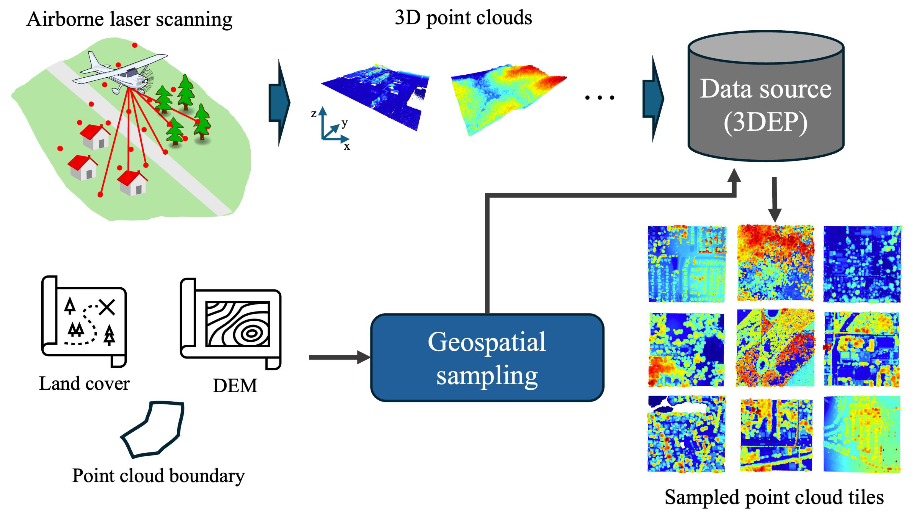
3.1. Framework Design
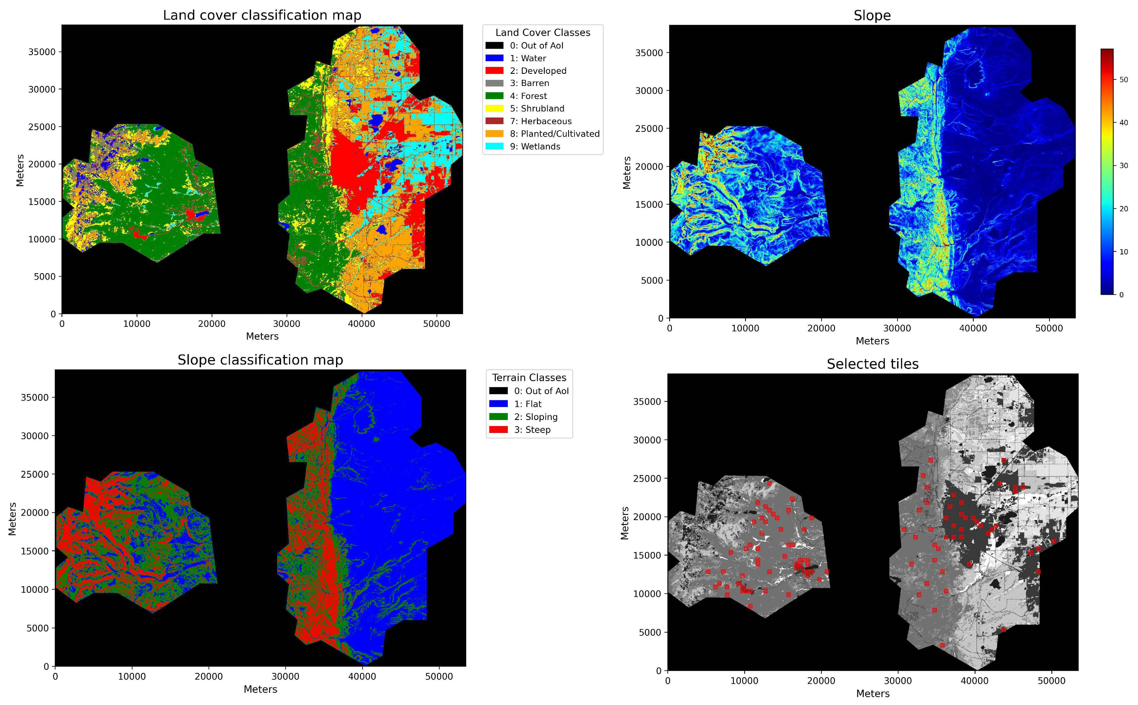
3.1.1. Land Cover and Terrain Information
3.1.2. Joint Land Cover–Terrain Inverse Probability Sampling
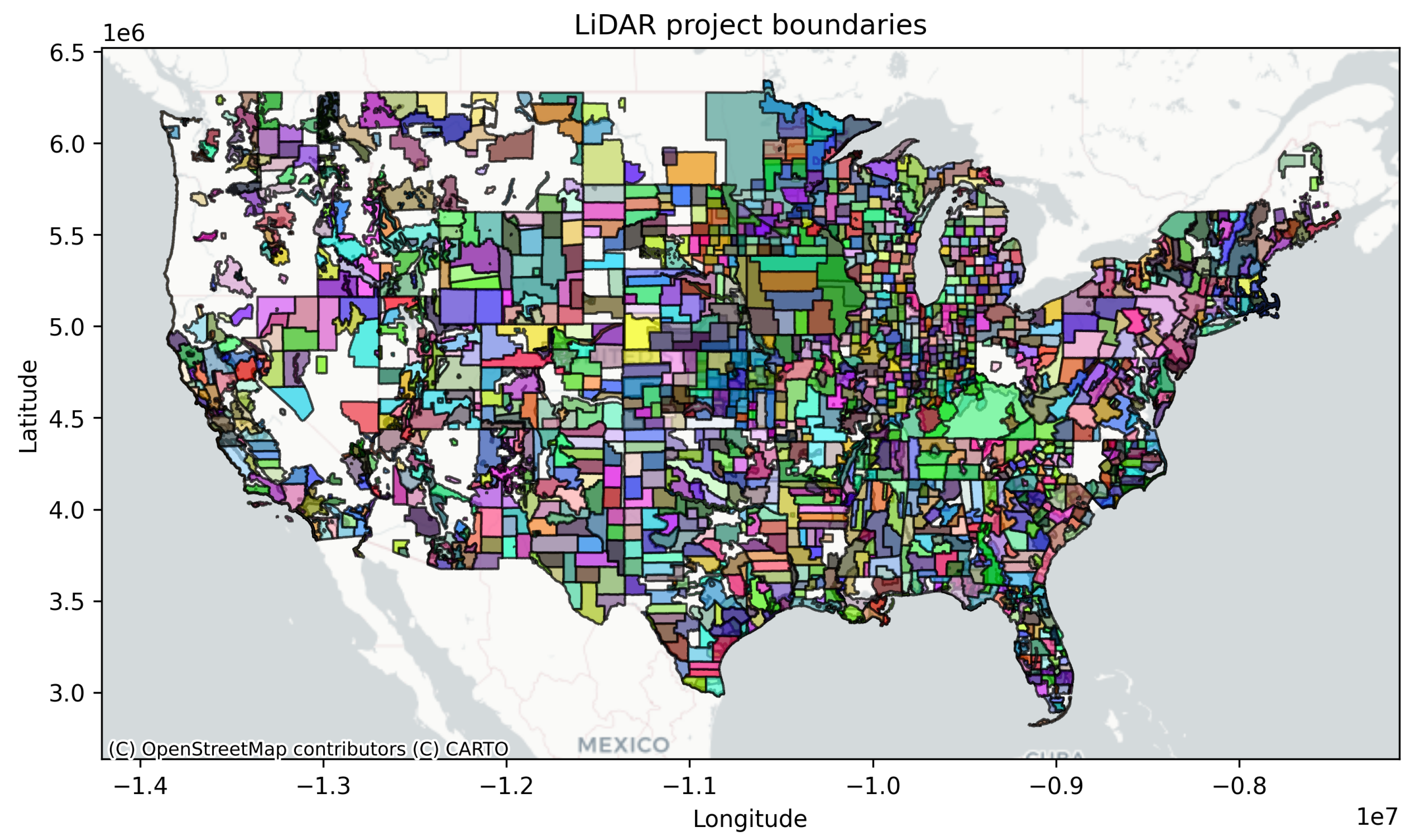
3.2. Data Source
3.2.1. LiDAR Point Cloud
3.2.2. Land Cover and Terrain Information
3.3. Framework Instantiation
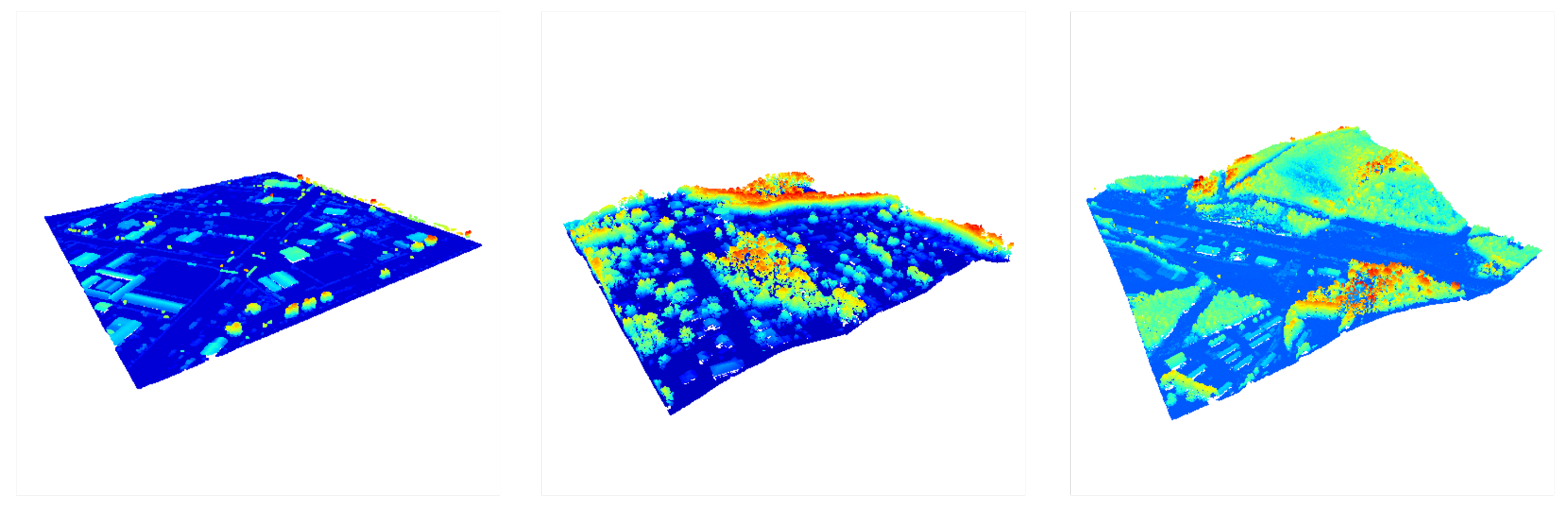
3.3.1. Data Processing and Sampling Details
3.3.2. Dataset Statistics and Comparison
4. Dataset Validation
4.1. Point Density
4.2. Ground Point Standard Deviation
4.3. Return Characteristics
5. Experiments
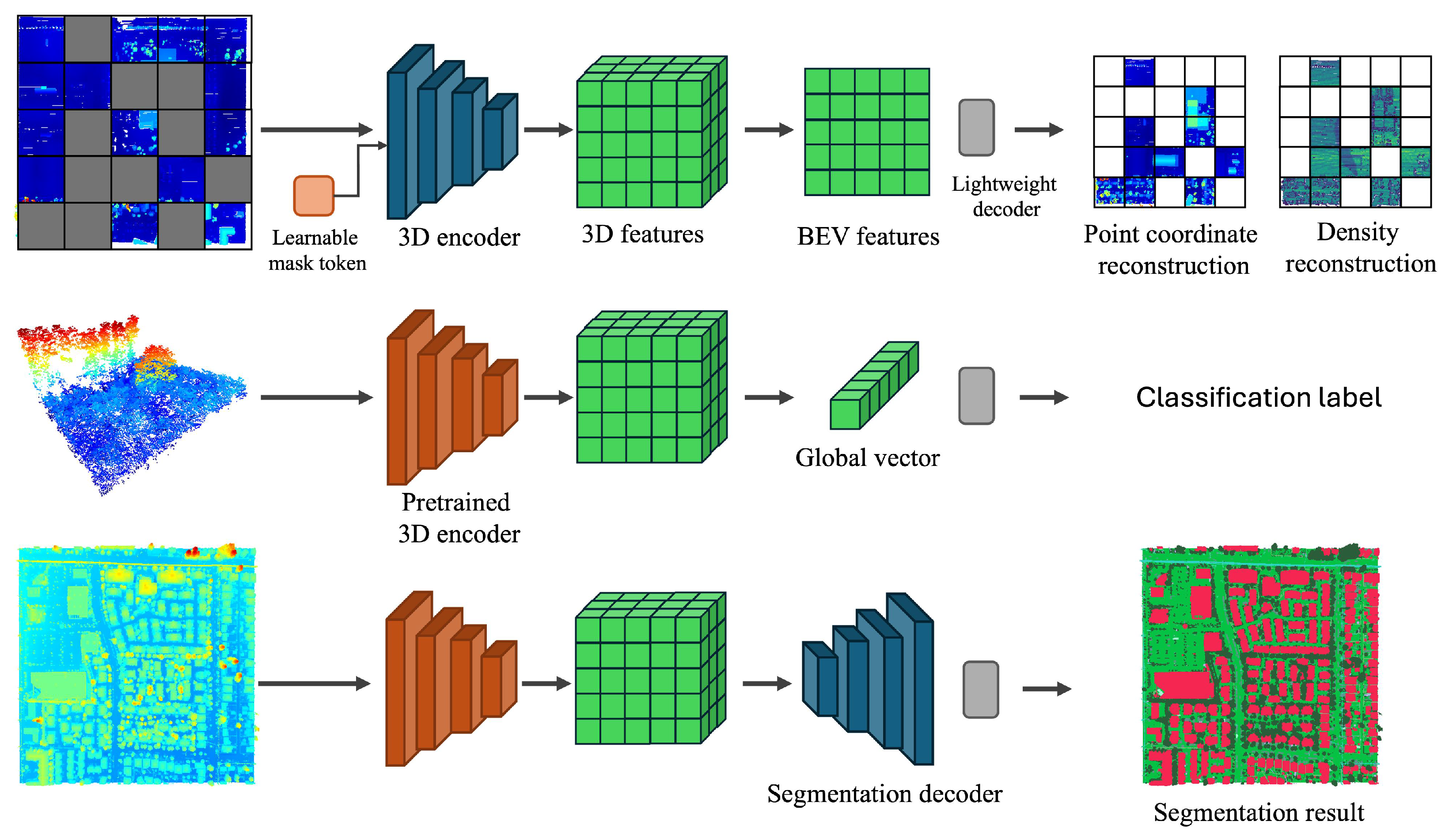
5.1. Model Architecture and Pre-Training
5.1.1. Model Description
5.1.2. Implementation Details for Pre-Training
5.2. Task
5.2.1. Tree Species Classification
5.2.2. Terrain Scene Recognition
5.2.3. Point Cloud Semantic Segmentation
5.3. Evaluation Metrics
6. Results
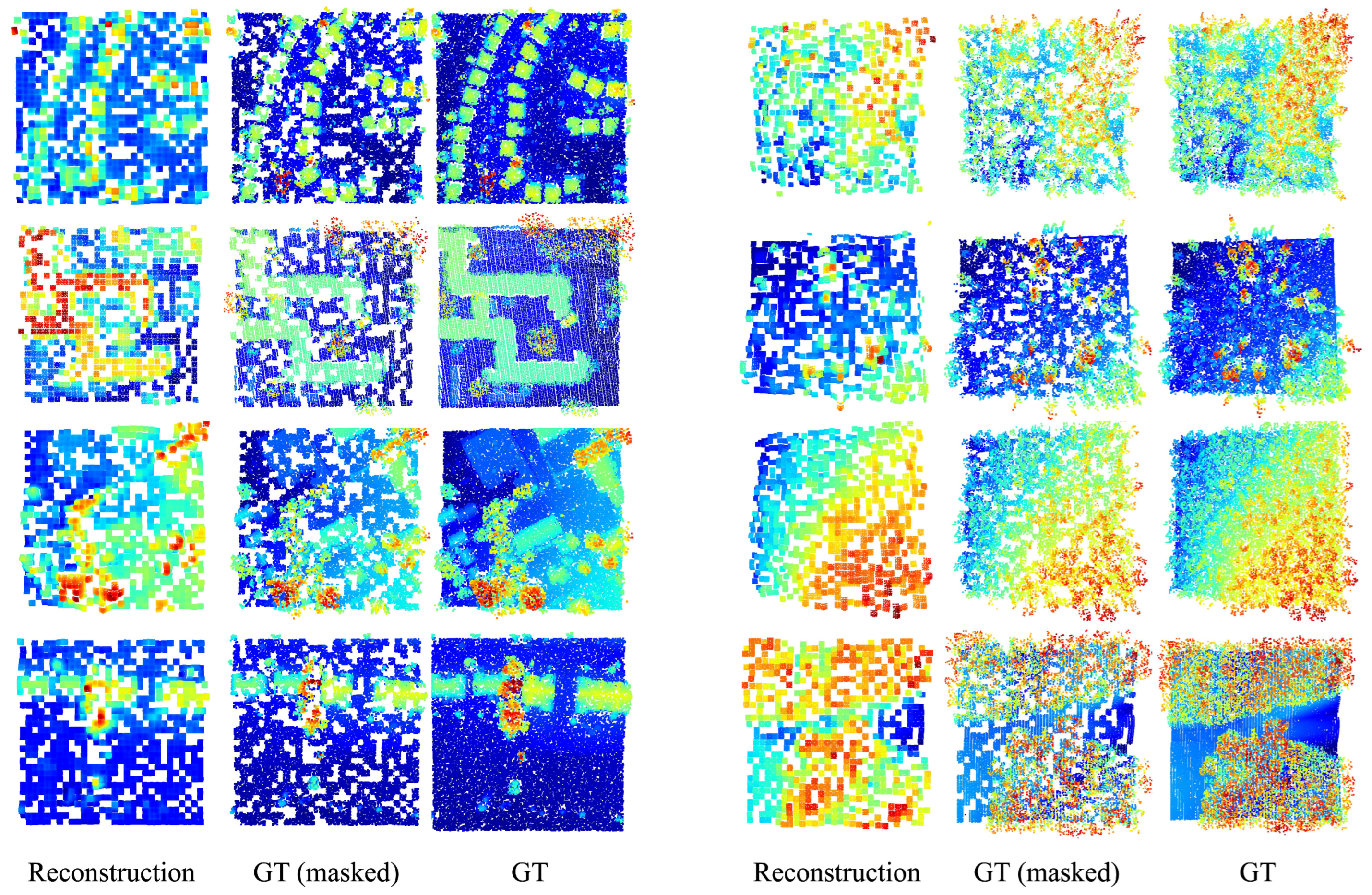
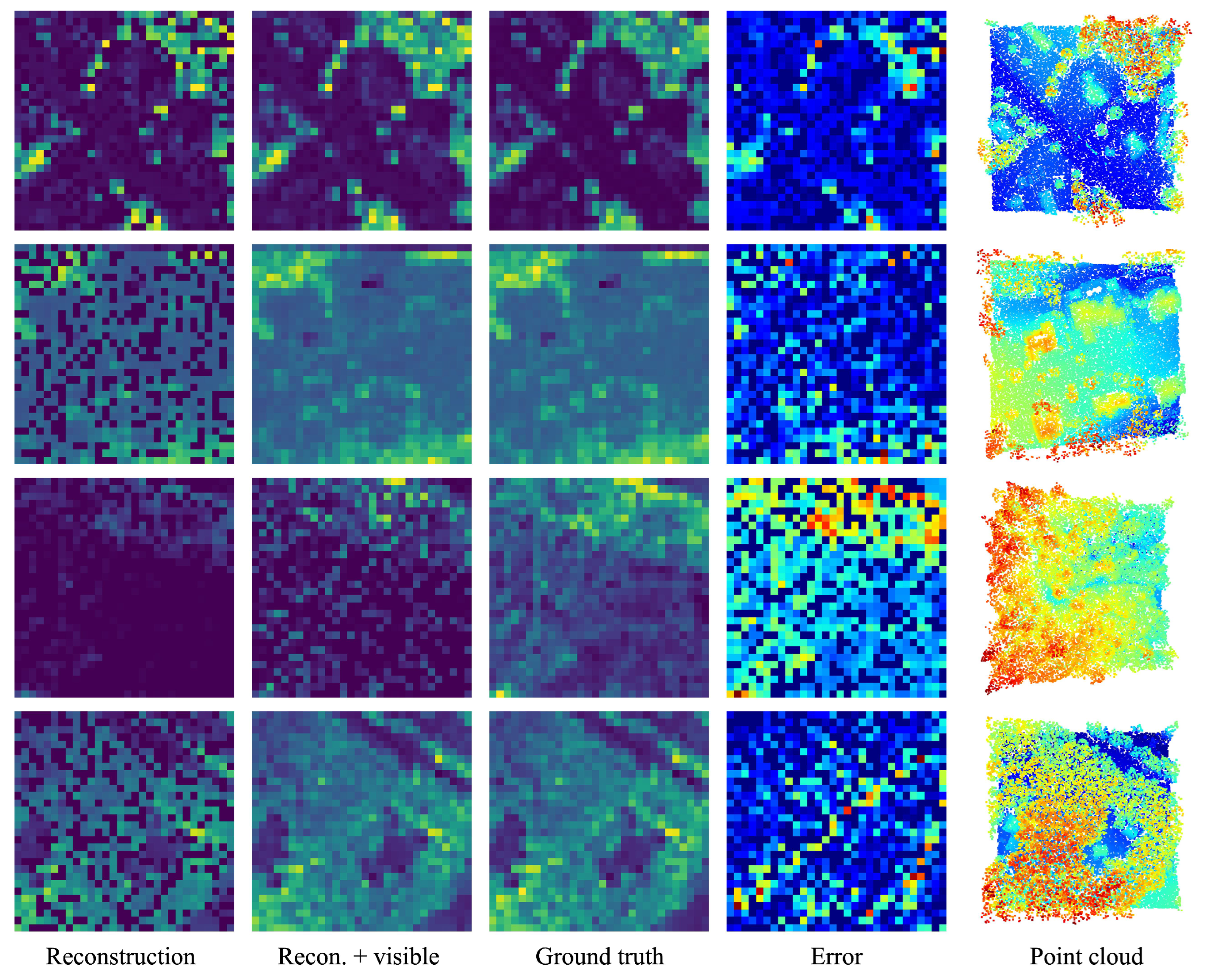
6.1. Pre-Training Results
6.2. Downstream Application Results
6.2.1. Tree Species Classification
6.2.2. Terrain Scene Recognition
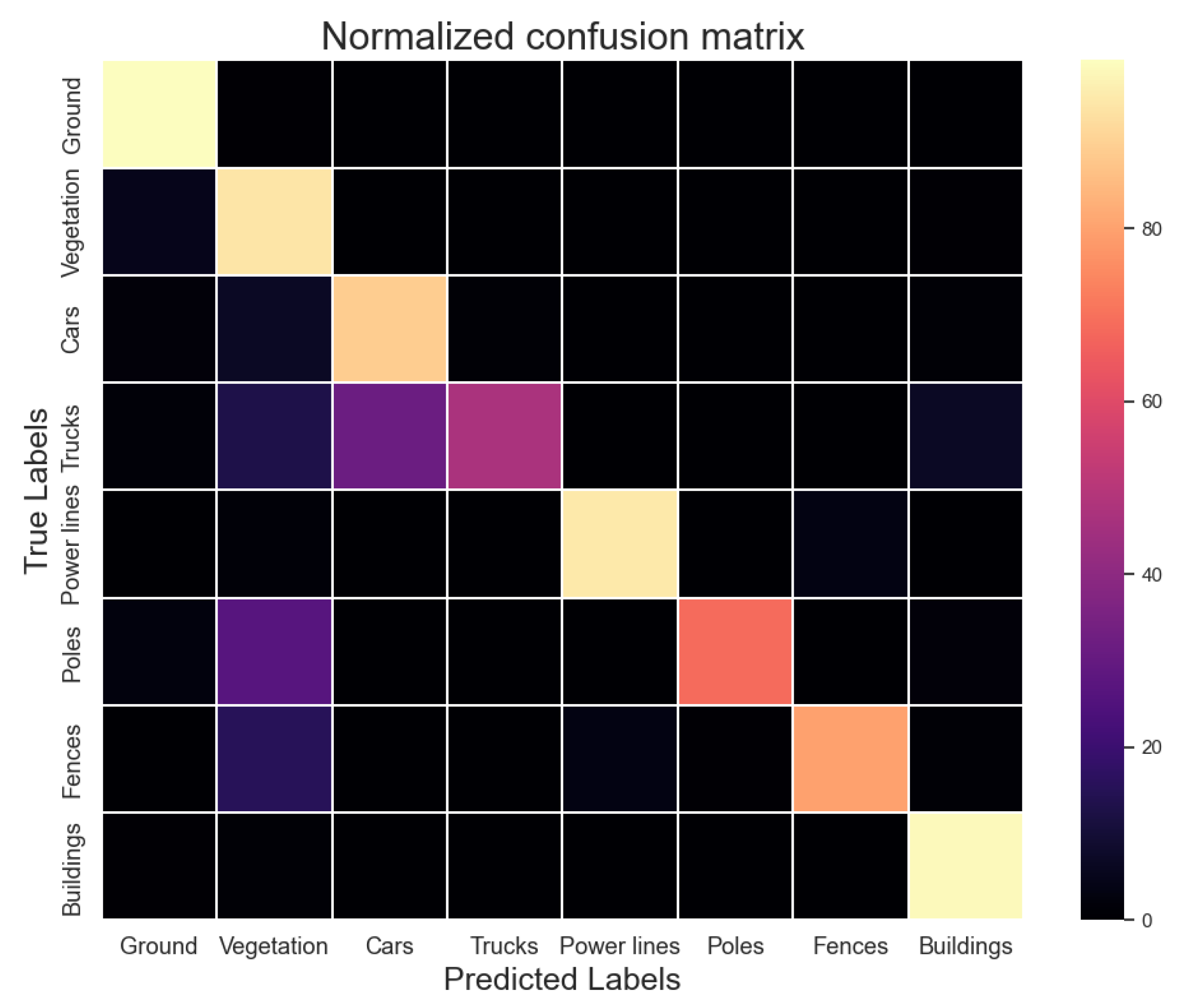
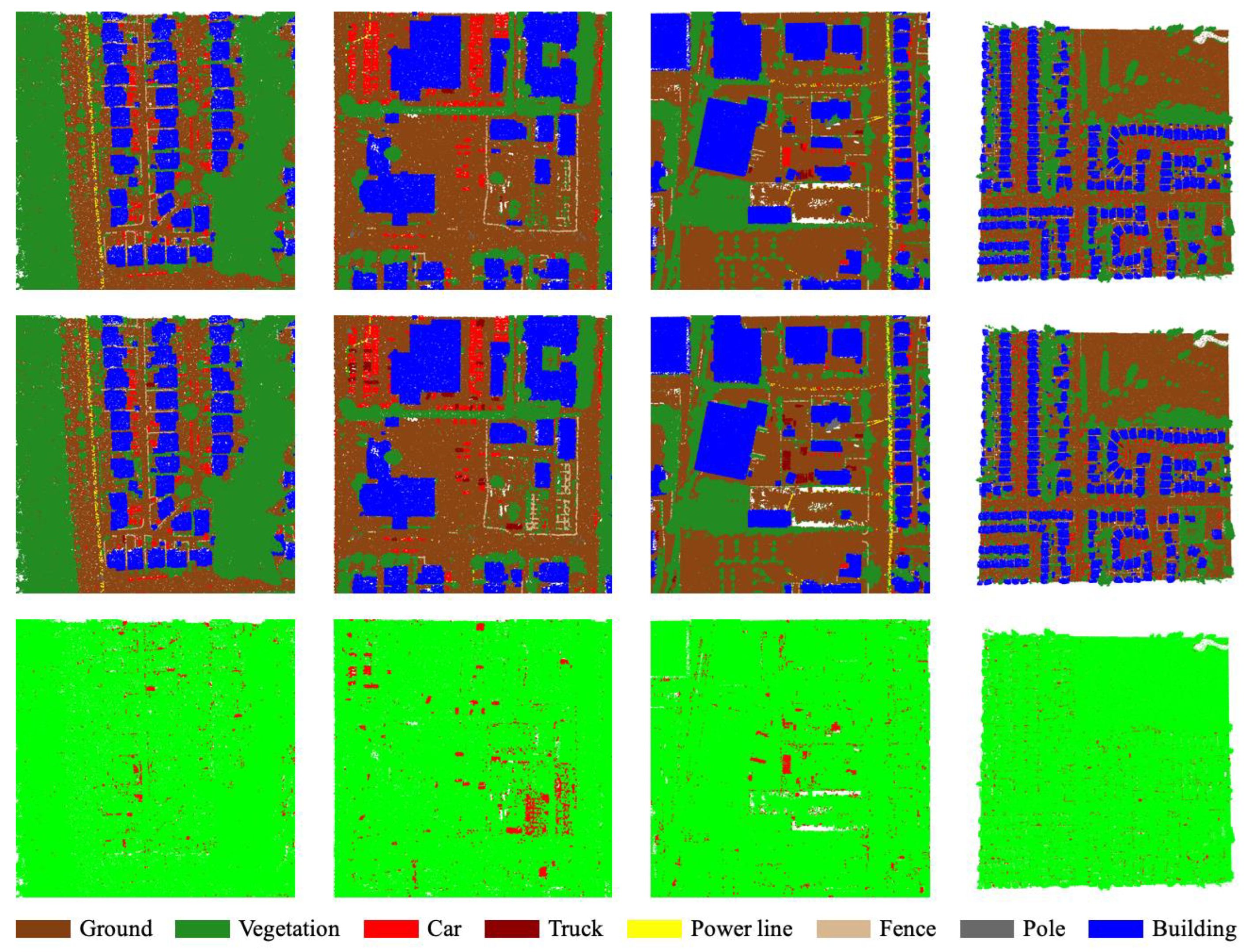
6.2.3. Point Cloud Semantic Segmentation for Developed Areas
7. Conclusions
Author Contributions
Funding
Data Availability Statement
Acknowledgments
Conflicts of Interest
References
- Qin, N.; Tan, W.; Ma, L.; Zhang, D.; Li, J. OpenGF: An ultra-large-scale ground filtering dataset built upon open ALS point clouds around the world. In Proceedings of the IEEE/CVF Conference on Computer Vision and Pattern Recognition, Virtual, 19–25 June 2021; pp. 1082–1091. [Google Scholar]
- Gaydon, C.; Roche, F. PureForest: A Large-scale Aerial Lidar and Aerial Imagery Dataset for Tree Species Classification in Monospecific Forests. arXiv 2024, arXiv:2404.12064. [Google Scholar]
- Varney, N.; Asari, V.K.; Graehling, Q. DALES: A large-scale aerial LiDAR data set for semantic segmentation. In Proceedings of the IEEE/CVF Conference on Computer Vision and Pattern Recognition Workshops, Virtual, 14–19 June 2020; pp. 186–187. [Google Scholar]
- Xiu, H.; Liu, X.; Wang, W.; Kim, K.S.; Shinohara, T.; Chang, Q.; Matsuoka, M. DS-Net: A dedicated approach for collapsed building detection from post-event airborne point clouds. Int. J. Appl. Earth Obs. Geoinf. 2023, 116, 103150. [Google Scholar] [CrossRef]
- Brown, T.; Mann, B.; Ryder, N.; Subbiah, M.; Kaplan, J.D.; Dhariwal, P.; Neelakantan, A.; Shyam, P.; Sastry, G.; Askell, A.; et al. Language models are few-shot learners. Adv. Neural Inf. Process. Syst. 2020, 33, 1877–1901. [Google Scholar]
- Radford, A.; Kim, J.W.; Hallacy, C.; Ramesh, A.; Goh, G.; Agarwal, S.; Sastry, G.; Askell, A.; Mishkin, P.; Clark, J.; et al. Learning transferable visual models from natural language supervision. In Proceedings of the International Conference on Machine Learning, PMLR, Virtual, 18–24 July 2021; pp. 8748–8763. [Google Scholar]
- Bommasani, R.; Hudson, D.A.; Adeli, E.; Altman, R.; Arora, S.; von Arx, S.; Bernstein, M.S.; Bohg, J.; Bosselut, A.; Brunskill, E.; et al. On the opportunities and risks of foundation models. arXiv 2021, arXiv:2108.07258. [Google Scholar]
- Guo, X.; Lao, J.; Dang, B.; Zhang, Y.; Yu, L.; Ru, L.; Zhong, L.; Huang, Z.; Wu, K.; Hu, D.; et al. Skysense: A multi-modal remote sensing foundation model towards universal interpretation for earth observation imagery. In Proceedings of the IEEE/CVF Conference on Computer Vision and Pattern Recognition, Seattle, WA, USA, 17–21 June 2024; pp. 27672–27683. [Google Scholar]
- Mendieta, M.; Han, B.; Shi, X.; Zhu, Y.; Chen, C. Towards geospatial foundation models via continual pretraining. In Proceedings of the IEEE/CVF International Conference on Computer Vision, Paris, France, 2–6 October 2023; pp. 16806–16816. [Google Scholar]
- Hong, D.; Zhang, B.; Li, X.; Li, Y.; Li, C.; Yao, J.; Yokoya, N.; Li, H.; Ghamisi, P.; Jia, X.; et al. SpectralGPT: Spectral remote sensing foundation model. IEEE Trans. Pattern Anal. Mach. Intell. 2024, 46, 5227–5244. [Google Scholar] [CrossRef]
- Stoker, J.; Miller, B. The accuracy and consistency of 3d elevation program data: A systematic analysis. Remote Sens. 2022, 14, 940. [Google Scholar] [CrossRef]
- Actueel Hoogtebestand Nederland. Actueel Hoogtebestand Nederland (AHN), n.d. Available online: https://www.ahn.nl/ (accessed on 26 December 2024).
- Lin, Z.; Wang, Y.; Qi, S.; Dong, N.; Yang, M.H. BEV-MAE: Bird’s Eye View Masked Autoencoders for Point Cloud Pre-training in Autonomous Driving Scenarios. In Proceedings of the AAAI Conference on Artificial Intelligence, Vancouver, BC, Canada, 20–27 February 2024; Volume 38, pp. 3531–3539. [Google Scholar]
- Liu, H.; Li, C.; Wu, Q.; Lee, Y.J. Visual instruction tuning. Adv. Neural Inf. Process. Syst. 2024, 36. [Google Scholar]
- Ayush, K.; Uzkent, B.; Meng, C.; Tanmay, K.; Burke, M.; Lobell, D.; Ermon, S. Geography-aware self-supervised learning. In Proceedings of the IEEE/CVF International Conference on Computer Vision, Virtual, 11–17 October 2021; pp. 10181–10190. [Google Scholar]
- Manas, O.; Lacoste, A.; Giró-i Nieto, X.; Vazquez, D.; Rodriguez, P. Seasonal contrast: Unsupervised pre-training from uncurated remote sensing data. In Proceedings of the IEEE/CVF International Conference on Computer Vision, virtual, 11–17 October 2021; pp. 9414–9423. [Google Scholar]
- Mall, U.; Hariharan, B.; Bala, K. Change-aware sampling and contrastive learning for satellite images. In Proceedings of the IEEE/CVF Conference on Computer Vision and Pattern Recognition, Vancouver, BC, Canada, 18–22 June 2023; pp. 5261–5270. [Google Scholar]
- Chen, X.; Fan, H.; Girshick, R.; He, K. Improved baselines with momentum contrastive learning. arXiv 2020, arXiv:2003.04297. [Google Scholar]
- He, K.; Chen, X.; Xie, S.; Li, Y.; Dollár, P.; Girshick, R. Masked autoencoders are scalable vision learners. In Proceedings of the IEEE/CVF Conference on Computer Vision and Pattern Recognition, New Orleans, LA, USA, 19–24 June 2022; pp. 16000–16009. [Google Scholar]
- Cong, Y.; Khanna, S.; Meng, C.; Liu, P.; Rozi, E.; He, Y.; Burke, M.; Lobell, D.; Ermon, S. Satmae: Pre-training transformers for temporal and multi-spectral satellite imagery. Adv. Neural Inf. Process. Syst. 2022, 35, 197–211. [Google Scholar]
- Sun, X.; Wang, P.; Lu, W.; Zhu, Z.; Lu, X.; He, Q.; Li, J.; Rong, X.; Yang, Z.; Chang, H.; et al. RingMo: A remote sensing foundation model with masked image modeling. IEEE Trans. Geosci. Remote Sens. 2022, 61, 1–22. [Google Scholar] [CrossRef]
- Deng, J.; Dong, W.; Socher, R.; Li, L.J.; Li, K.; Fei-Fei, L. Imagenet: A large-scale hierarchical image database. In Proceedings of the 2009 IEEE Conference on Computer Vision and Pattern Recognition, Miami, FL, USA, 20–25 June 2009; IEEE: Piscataway, NJ, USA, 2009; pp. 248–255. [Google Scholar]
- Han, B.; Zhang, S.; Shi, X.; Reichstein, M. Bridging remote sensors with multisensor geospatial foundation models. In Proceedings of the IEEE/CVF Conference on Computer Vision and Pattern Recognition, Seattle, WA, USA, 17–21 June 2024; pp. 27852–27862. [Google Scholar]
- Liu, F.; Chen, D.; Guan, Z.; Zhou, X.; Zhu, J.; Ye, Q.; Fu, L.; Zhou, J. Remoteclip: A vision language foundation model for remote sensing. IEEE Trans. Geosci. Remote Sens. 2024, 62, 5622216. [Google Scholar] [CrossRef]
- Wang, Z.; Prabha, R.; Huang, T.; Wu, J.; Rajagopal, R. Skyscript: A large and semantically diverse vision-language dataset for remote sensing. In Proceedings of the AAAI Conference on Artificial Intelligence, Vancouver, BC, Canada, 20–27 February 2024; Volume 38, pp. 5805–5813. [Google Scholar]
- Mall, U.; Phoo, C.P.; Liu, M.K.; Vondrick, C.; Hariharan, B.; Bala, K. Remote sensing vision-language foundation models without annotations via ground remote alignment. arXiv 2023, arXiv:2312.06960. [Google Scholar]
- Kuckreja, K.; Danish, M.S.; Naseer, M.; Das, A.; Khan, S.; Khan, F.S. Geochat: Grounded large vision-language model for remote sensing. In Proceedings of the IEEE/CVF Conference on Computer Vision and Pattern Recognition, Seattle, WA, USA, 17–21 June 2024; pp. 27831–27840. [Google Scholar]
- Liu, H.; Li, C.; Li, Y.; Lee, Y.J. Improved baselines with visual instruction tuning. In Proceedings of the IEEE/CVF Conference on Computer Vision and Pattern Recognition, Seattle, WA, USA, 17–21 June 2024; pp. 26296–26306. [Google Scholar]
- Li, X.; Li, C.; Tong, Z.; Lim, A.; Yuan, J.; Wu, Y.; Tang, J.; Huang, R. Campus3d: A photogrammetry point cloud benchmark for hierarchical understanding of outdoor scene. In Proceedings of the 28th ACM International Conference on Multimedia, Seattle, WA, USA, 12–16 October 2020; pp. 238–246. [Google Scholar]
- Hu, Q.; Yang, B.; Khalid, S.; Xiao, W.; Trigoni, N.; Markham, A. Sensaturban: Learning semantics from urban-scale photogrammetric point clouds. Int. J. Comput. Vis. 2022, 130, 316–343. [Google Scholar] [CrossRef]
- Li, M.; Wu, Y.; Yeh, A.G.; Xue, F. HRHD-HK: A benchmark dataset of high-rise and high-density urban scenes for 3D semantic segmentation of photogrammetric point clouds. In Proceedings of the 2023 IEEE International Conference on Image Processing Challenges and Workshops (ICIPCW), Kuala Lumpur, Malaysia, 8–11 October 2023; Volume 1, pp. 3714–3718. [Google Scholar]
- Chen, M.; Hu, Q.; Yu, Z.; Thomas, H.; Feng, A.; Hou, Y.; McCullough, K.; Ren, F.; Soibelman, L. Stpls3d: A large-scale synthetic and real aerial photogrammetry 3d point cloud dataset. arXiv 2022, arXiv:2203.09065. [Google Scholar]
- Hackel, T.; Savinov, N.; Ladicky, L.; Wegner, J.D.; Schindler, K.; Pollefeys, M. Semantic3d. net: A new large-scale point cloud classification benchmark. arXiv 2017, arXiv:1704.03847. [Google Scholar]
- Roynard, X.; Deschaud, J.E.; Goulette, F. Paris-Lille-3D: A large and high-quality ground-truth urban point cloud dataset for automatic segmentation and classification. Int. J. Robot. Res. 2018, 37, 545–557. [Google Scholar] [CrossRef]
- Behley, J.; Garbade, M.; Milioto, A.; Quenzel, J.; Behnke, S.; Stachniss, C.; Gall, J. Semantickitti: A dataset for semantic scene understanding of lidar sequences. In Proceedings of the IEEE/CVF International Conference on Computer Vision, Seoul, Republic of Korea, 27 October–2 November 2019; pp. 9297–9307. [Google Scholar]
- Tan, W.; Qin, N.; Ma, L.; Li, Y.; Du, J.; Cai, G.; Yang, K.; Li, J. Toronto-3D: A large-scale mobile LiDAR dataset for semantic segmentation of urban roadways. In Proceedings of the IEEE/CVF Conference on Computer Vision and Pattern Recognition Workshops, Seattle, WA, USA, 14–19 June 2020; pp. 202–203. [Google Scholar]
- Rottensteiner, F.; Sohn, G.; Gerke, M.; Wegner, J.D.; Breitkopf, U.; Jung, J. Results of the ISPRS benchmark on urban object detection and 3D building reconstruction. ISPRS J. Photogramm. Remote Sens. 2014, 93, 256–271. [Google Scholar] [CrossRef]
- Zolanvari, S.; Ruano, S.; Rana, A.; Cummins, A.; Da Silva, R.E.; Rahbar, M.; Smolic, A. DublinCity: Annotated LiDAR point cloud and its applications. arXiv 2019, arXiv:1909.03613. [Google Scholar]
- Ye, Z.; Xu, Y.; Huang, R.; Tong, X.; Li, X.; Liu, X.; Luan, K.; Hoegner, L.; Stilla, U. Lasdu: A large-scale aerial lidar dataset for semantic labeling in dense urban areas. ISPRS Int. J. -Geo-Inf. 2020, 9, 450. [Google Scholar] [CrossRef]
- Devlin, J. Bert: Pre-training of deep bidirectional transformers for language understanding. arXiv 2018, arXiv:1810.04805. [Google Scholar]
- Yu, X.; Tang, L.; Rao, Y.; Huang, T.; Zhou, J.; Lu, J. Point-bert: Pre-training 3d point cloud transformers with masked point modeling. In Proceedings of the IEEE/CVF Conference on Computer Vision and Pattern Recognition, New Orleans, LA, USA, 19–24 June 2022; pp. 19313–19322. [Google Scholar]
- Fu, K.; Gao, P.; Liu, S.; Qu, L.; Gao, L.; Wang, M. Pos-bert: Point cloud one-stage bert pre-training. Expert Syst. Appl. 2024, 240, 122563. [Google Scholar] [CrossRef]
- Fu, K.; Yuan, M.; Liu, S.; Wang, M. Boosting point-bert by multi-choice tokens. IEEE Trans. Circuits Syst. Video Technol. 2023, 34, 438–447. [Google Scholar] [CrossRef]
- Rolfe, J.T. Discrete Variational Autoencoders. arXiv 2017, arXiv:1609.02200. [Google Scholar]
- Pang, Y.; Wang, W.; Tay, F.E.; Liu, W.; Tian, Y.; Yuan, L. Masked autoencoders for point cloud self-supervised learning. In Proceedings of the European Conference on Computer Vision, Tel Aviv, Israel, 23–27 October 2022; Springer: Berlin/Heidelberg, Germany, 2022; pp. 604–621. [Google Scholar]
- Liu, H.; Cai, M.; Lee, Y.J. Masked discrimination for self-supervised learning on point clouds. In Proceedings of the European Conference on Computer Vision, Tel Aviv, Israel, 23–27 October 2022; Springer: Berlin/Heidelberg, Germany, 2022; pp. 657–675. [Google Scholar]
- Zhang, R.; Guo, Z.; Gao, P.; Fang, R.; Zhao, B.; Wang, D.; Qiao, Y.; Li, H. Point-m2ae: Multi-scale masked autoencoders for hierarchical point cloud pre-training. Adv. Neural Inf. Process. Syst. 2022, 35, 27061–27074. [Google Scholar]
- Chen, G.; Wang, M.; Yang, Y.; Yu, K.; Yuan, L.; Yue, Y. Pointgpt: Auto-regressively generative pre-training from point clouds. Adv. Neural Inf. Process. Syst. 2023, 36, 29667–29679. [Google Scholar]
- Yan, S.; Yang, Y.; Guo, Y.; Pan, H.; Wang, P.s.; Tong, X.; Liu, Y.; Huang, Q. 3d feature prediction for masked-autoencoder-based point cloud pretraining. arXiv 2023, arXiv:2304.06911. [Google Scholar]
- Zhang, R.; Wang, L.; Qiao, Y.; Gao, P.; Li, H. Learning 3d representations from 2d pre-trained models via image-to-point masked autoencoders. In Proceedings of the IEEE/CVF Conference on Computer Vision and Pattern Recognition, Vancouver, BC, Canada, 18–22 June 2023; pp. 21769–21780. [Google Scholar]
- Guo, Z.; Zhang, R.; Qiu, L.; Li, X.; Heng, P.A. Joint-mae: 2D-3D joint masked autoencoders for 3d point cloud pre-training. arXiv 2023, arXiv:2302.14007. [Google Scholar]
- Qi, Z.; Dong, R.; Fan, G.; Ge, Z.; Zhang, X.; Ma, K.; Yi, L. Contrast with reconstruct: Contrastive 3d representation learning guided by generative pretraining. In Proceedings of the International Conference on Machine Learning, PMLR, Honolulu, HI, USA, 23–29 July 2023; pp. 28223–28243. [Google Scholar]
- Hess, G.; Jaxing, J.; Svensson, E.; Hagerman, D.; Petersson, C.; Svensson, L. Masked autoencoder for self-supervised pre-training on lidar point clouds. In Proceedings of the IEEE/CVF Winter Conference on Applications of Computer Vision, Waikoloa, HI, USA, 3–7 January 2023; pp. 350–359. [Google Scholar]
- Tian, X.; Ran, H.; Wang, Y.; Zhao, H. Geomae: Masked geometric target prediction for self-supervised point cloud pre-training. In Proceedings of the IEEE/CVF Conference on Computer Vision and Pattern Recognition, Vancouver, BC, Canada, 18–22 June 2023; pp. 13570–13580. [Google Scholar]
- Yang, H.; He, T.; Liu, J.; Chen, H.; Wu, B.; Lin, B.; He, X.; Ouyang, W. GD-MAE: Generative decoder for MAE pre-training on lidar point clouds. In Proceedings of the PIEEE/CVF Conference on Computer Vision and Pattern Recognition, Vancouver, BC, Canada, 18–22 June 2023; pp. 9403–9414. [Google Scholar]
- Carós, M.; Just, A.; Seguí, S.; Vitrià, J. Self-Supervised Pre-Training Boosts Semantic Scene Segmentation on LiDAR data. In Proceedings of the 2023 18th International Conference on Machine Vision and Applications (MVA), Hamamatsu, Japan, 23–25 July 2023; IEEE: Piscataway, NJ, USA, 2023; pp. 1–6. [Google Scholar]
- Zbontar, J.; Jing, L.; Misra, I.; LeCun, Y.; Deny, S. Barlow twins: Self-supervised learning via redundancy reduction. In Proceedings of the International Conference on Machine Learning, PMLR, Virtual Event, 18–24 July 2021; pp. 12310–12320. [Google Scholar]
- de Gélis, I.; Saha, S.; Shahzad, M.; Corpetti, T.; Lefèvre, S.; Zhu, X.X. Deep unsupervised learning for 3d als point clouds change detection. ISPRS Open J. Photogramm. Remote Sens. 2023, 9, 100044. [Google Scholar] [CrossRef]
- Yang, H.; Huang, S.; Wang, R.; Wang, X. Self-Supervised Pre-Training for 3D Roof Reconstruction on LiDAR Data. IEEE Geosci. Remote Sens. Lett. 2024, 21, 6500405. [Google Scholar]
- Zhang, Y.; Yao, J.; Zhang, R.; Wang, X.; Chen, S.; Fu, H. HAVANA: Hard Negative Sample-Aware Self-Supervised Contrastive Learning for Airborne Laser Scanning Point Cloud Semantic Segmentation. Remote Sens. 2024, 16, 485. [Google Scholar] [CrossRef]
- U.S. Geological Survey. What is 3DEP? 2024. Available online: https://www.usgs.gov/3d-elevation-program/what-3dep (accessed on 2 December 2024).
- U.S. Geological Survey. USGS 3DEP LiDAR Point Clouds. 2024. Available online: https://registry.opendata.aws/usgs-lidar/ (accessed on 2 December 2024).
- Wickham, J.; Stehman, S.V.; Sorenson, D.G.; Gass, L.; Dewitz, J.A. Thematic accuracy assessment of the NLCD 2019 land cover for the conterminous United States. Gisci. Remote Sens. 2023, 60, 2181143. [Google Scholar] [CrossRef] [PubMed]
- Multi-Resolution Land Characteristics (MRLC) Consortium. National Land Cover Database Class Legend and Description. 2024. Available online: https://www.mrlc.gov/data/legends/national-land-cover-database-class-legend-and-description (accessed on 3 December 2024).
- Pamela, P.; Yukni, A.; Imam, S.A.; Kartiko, R.D. The selective causative factors on landslide susceptibility assessment: Case study Takengon, Aceh, Indonesia. In Proceedings of the AIP Conference Proceedings, Maharashtra, India, 5–6 July 2018; AIP Publishing: Melville, NY, USA, 2018; Volume 1987. [Google Scholar]
- Chegini, T.; Li, H.Y.; Leung, L.R. HyRiver: Hydroclimate Data Retriever. J. Open Source Softw. 2021, 6, 1–3. [Google Scholar] [CrossRef]
- U.S. Geological Survey. Thematic Accuracy Assessment of NLCD 2019 Land Cover for the Conterminous United States. 2024. Available online: https://www.usgs.gov/publications/thematic-accuracy-assessment-nlcd-2019-land-cover-conterminous-united-states (accessed on 2 December 2024).
- Melekhov, I.; Umashankar, A.; Kim, H.J.; Serkov, V.; Argyle, D. ECLAIR: A High-Fidelity Aerial LiDAR Dataset for Semantic Segmentation. In Proceedings of the IEEE/CVF Conference on Computer Vision and Pattern Recognition, Seattle, WA, USA, 17–21 June 2024; pp. 7627–7637. [Google Scholar]
- Graves, S.; Marconi, S. IDTReeS 2020 Competition Data. 2020. Available online: https://zenodo.org/records/3700197 (accessed on 23 May 2025).
- Sithole, G.; Vosselman, G. Experimental comparison of filter algorithms for bare-Earth extraction from airborne laser scanning point clouds. ISPRS J. Photogramm. Remote Sens. 2004, 59, 85–101. [Google Scholar] [CrossRef]
- Graham, B.; Engelcke, M.; Van Der Maaten, L. 3d semantic segmentation with submanifold sparse convolutional networks. In Proceedings of the IEEE Conference on Computer Vision and Pattern Recognition, Salt Lake City, UT, USA, 18–22 June 2018; pp. 9224–9232. [Google Scholar]
- Choy, C.; Gwak, J.; Savarese, S. 4D spatio-temporal convnets: Minkowski convolutional neural networks. In Proceedings of the IEEE/CVF Conference on Computer Vision and Pattern Recognition, Long Beach, CA, USA, 16–20 June 2019; pp. 3075–3084. [Google Scholar]
- Qin, N.; Hu, X.; Dai, H. Deep fusion of multi-view and multimodal representation of ALS point cloud for 3D terrain scene recognition. ISPRS J. Photogramm. Remote Sens. 2018, 143, 205–212. [Google Scholar] [CrossRef]
- Ronneberger, O.; Fischer, P.; Brox, T. U-net: Convolutional networks for biomedical image segmentation. In Proceedings of the Medical Image Computing and Computer-Assisted Intervention—MICCAI 2015: 18th International Conference, Munich, Germany, 5–9 October 2015; Proceedings, Part III 18. Springer: Berlin/Heidelberg, Germany, 2015; pp. 234–241. [Google Scholar]
- Qi, C.R.; Su, H.; Mo, K.; Guibas, L.J. Pointnet: Deep learning on point sets for 3d classification and segmentation. In Proceedings of the IEEE Conference on Computer Vision and Pattern Recognition, Honolulu, HI, USA, 21–26 July 2017; pp. 652–660. [Google Scholar]
- Qi, C.R.; Yi, L.; Su, H.; Guibas, L.J. Pointnet++: Deep hierarchical feature learning on point sets in a metric space. Adv. Neural Inf. Process. Syst. 2017, 5105–5114. [Google Scholar]
- Chen, Y.; Liu, J.; Zhang, X.; Qi, X.; Jia, J. VoxelNeXt: Fully Sparse VoxelNet for 3D Object Detection and Tracking. In Proceedings of the IEEE/CVF Conference on Computer Vision and Pattern Recognition, Vancouver, BC, Canada, 18–22 June 2023. [Google Scholar]
- Thomas, H.; Qi, C.R.; Deschaud, J.E.; Marcotegui, B.; Goulette, F.; Guibas, L.J. Kpconv: Flexible and deformable convolution for point clouds. In Proceedings of the IEEE/CVF International Conference on Computer Vision, Long Beach, CA, USA, 16–20 June 2019; pp. 6411–6420. [Google Scholar]
- Hu, Q.; Yang, B.; Xie, L.; Rosa, S.; Guo, Y.; Wang, Z.; Trigoni, N.; Markham, A. Randla-net: Efficient semantic segmentation of large-scale point clouds. In Proceedings of the IEEE/CVF Conference on Computer Vision and Pattern Recognition, Virtual, 14–19 June 2020; pp. 11108–11117. [Google Scholar]
- Yoo, S.; Jeong, Y.; Jameela, M.; Sohn, G. Human vision based 3d point cloud semantic segmentation of large-scale outdoor scenes. In Proceedings of the IEEE/CVF Conference on Computer Vision and Pattern Recognition, Vancouver, BC, Canada, 18–22 June 2023; pp. 6577–6586. [Google Scholar]
- Tukra, S.; Hoffman, F.; Chatfield, K. Improving visual representation learning through perceptual understanding. In Proceedings of the IEEE/CVF Conference on Computer Vision and Pattern Recognition, Vancouver, BC, Canada, 18–22 June 2023; pp. 14486–14495. [Google Scholar]
- Reed, C.J.; Gupta, R.; Li, S.; Brockman, S.; Funk, C.; Clipp, B.; Keutzer, K.; Candido, S.; Uyttendaele, M.; Darrell, T. Scale-mae: A scale-aware masked autoencoder for multiscale geospatial representation learning. In Proceedings of the IEEE/CVF International Conference on Computer Vision, Vancouver, BC, Canada, 18–22 June 2023; pp. 4088–4099. [Google Scholar]

| Level I Class | Level II Class |
|---|---|
| Water | Open Water |
| Perennial Ice/Snow | |
| Developed | Developed, Open Space |
| Developed, Low Intensity | |
| Developed, Medium Intensity | |
| Developed, High Intensity | |
| Barren | Barren Land (Rock/Sand/Clay) |
| Forest | Deciduous Forest |
| Evergreen Forest | |
| Mixed Forest | |
| Shrubland | Dwarf Scrub (Alaska only) |
| Shrub/Scrub | |
| Herbaceous | Grassland/Herbaceous |
| Sedge/Herbaceous (Alaska only) | |
| Lichens (Alaska only) | |
| Moss (Alaska only) | |
| Planted/Cultivated | Pasture/Hay |
| Cultivated Crops | |
| Wetlands | Woody Wetlands |
| Emergent Herbaceous Wetlands |
| Slope Class | Degree | Percentage |
|---|---|---|
| Flat | 0–5° | 0–8.7% |
| Sloped | 5–17° | 8.7–30.6% |
| Steep | ≥17° | ≥30.6% |
| Developed | Forest | All | |
|---|---|---|---|
| Flat | 28,523 | 18,071 | 46,594 |
| Sloped | 3774 | 16,021 | 19,795 |
| Steep | 308 | 7065 | 7373 |
| All | 32,605 | 41,157 | 73,762 |
| Dataset | Year | Coverage | # Points | Land Cover Type |
|---|---|---|---|---|
| ISPRS [37] | 2014 | – | 1.2 M | Developed |
| DublinCity [38] | 2019 | 260 M | Developed | |
| LASDU [39] | 2020 | 3.12 M | Developed | |
| DALES [3] | 2020 | 505 M | Developed | |
| ECLAIR [68] | 2024 | 582 M | Developed | |
| IDTReeS [69] | 2021 | 0.02 M | Forest | |
| PureForest [2] | 2024 | 15 B | Forest | |
| ISPRS filtertest [70] | – | 0.4 M | Developed, Forest | |
| OpenGF [1] | 2021 | 542.1 M | Developed, Forest | |
| 3DEP (Ours) | - | 17,691 | 184 B | Developed, Forest |
| Developed | Forest | All | |
|---|---|---|---|
| Flat | 7.7/9.9 | 11.1/15.3 | 9.0/12.4 |
| Sloped | 11.2/16.0 | 11.9/15.5 | 11.8/15.6 |
| Steep | 28.0/39.6 | 18.0/19.2 | 18.4/20.5 |
| All | 8.2/11.6 | 12.6/16.3 | 10.7/14.6 |
| Developed | Forest | All | |
|---|---|---|---|
| Flat | 2.5/3.4 | 4.9/4.1 | 3.5/3.8 |
| Sloped | 12.7/6.1 | 14.7/8.7 | 14.4/8.3 |
| Steep | 36.1/18.8 | 43.6/19.1 | 43.3/19.1 |
| All | 4.0/6.1 | 15.3/16.8 | 10.4/14.4 |
| Return Number | Sum Point Count | Percent (%) of Total |
|---|---|---|
| Single | 13,036,774,317 | 67.92 |
| First | 15,495,147,301 | 80.73 |
| First of many | 2,446,338,594 | 12.74 |
| Second | 2,491,508,834 | 12.98 |
| Third | 839,493,704 | 4.37 |
| Fourth | 255,303,252 | 1.33 |
| Fifth | 71,200,968 | 0.37 |
| Sixth | 28,103,502 | 0.15 |
| Seventh | 14,103,705 | 0.07 |
| Last | 15,594,824,929 | 81.24 |
| Last of many | 2,559,449,009 | 13.33 |
| Return Number | Sum Point Count | Percen (%) of Total |
|---|---|---|
| Single | 27,509,188,124 | 49.32 |
| First | 38,520,832,462 | 69.07 |
| First of Many | 10,992,636,342 | 19.71 |
| Second | 11,082,071,467 | 19.87 |
| Third | 4,272,395,407 | 7.66 |
| Fourth | 1,369,446,735 | 2.46 |
| Fifth | 364,742,990 | 0.65 |
| Sixth | 115,577,887 | 0.21 |
| Seventh | 47,218,274 | 0.08 |
| Last | 38,817,185,224 | 69.60 |
| Last of Many | 11,310,467,287 | 20.28 |
| Method | mIoU (%) | OA (%) |
|---|---|---|
| Lidar (Baseline) [2] | 55.1 | 80.3 |
| Lidar + RGBI [2] | 53.6 | 79.1 |
| Lidar + Elevation [2] | 57.2 | 83.6 |
| Aerial Imagery [2] | 50.0 | 73.1 |
| BEV-MAE (Scratch) | 72.2 | 86.8 |
| BEV-MAE (Ours) | 75.6 | 87.1 |
| Category | # Tiles | Lidar (Baseline) | Scratch | Ours |
|---|---|---|---|---|
| Deciduous oak | 48,055 | 73.4 | 78.3 | 78.5 |
| Evergreen oak | 22,361 | 59.4 | 63.2 | 63.7 |
| Beech | 12,670 | 88.8 | 93.1 | 92.2 |
| Chestnut | 3684 | 56.5 | 65.6 | 62.0 |
| Black locust | 2303 | 58.1 | 73.7 | 82.2 |
| Maritime pine | 7568 | 62.9 | 96.2 | 97.5 |
| Scotch pine | 18,265 | 58.6 | 86.7 | 88.2 |
| Black pine | 7226 | 46.2 | 74.3 | 79.0 |
| Aleppo pine | 4699 | 39.3 | 87.9 | 93.7 |
| Fir | 840 | 0.0 | 0.0 | 0.0 |
| Spruce | 4074 | 85.8 | 94.2 | 93.3 |
| Larch | 3294 | 50.6 | 81.7 | 85.6 |
| Douglas | 530 | 36.5 | 78.8 | 93.3 |
| Mean | – | 55.1 | 74.9 | 77.6 |
| Method | mIoU (%) | OA (%) |
|---|---|---|
| PointNet [75] | 65.0 | 77.6 |
| PointNet++ [76] | 87.6 | 93.1 |
| VoxelNeXt [77] | 86.6 | 92.6 |
| BEV-MAE (Scratch) | 86.6 | 92.6 |
| BEV-MAE (Ours) | 87.4 | 93.1 |
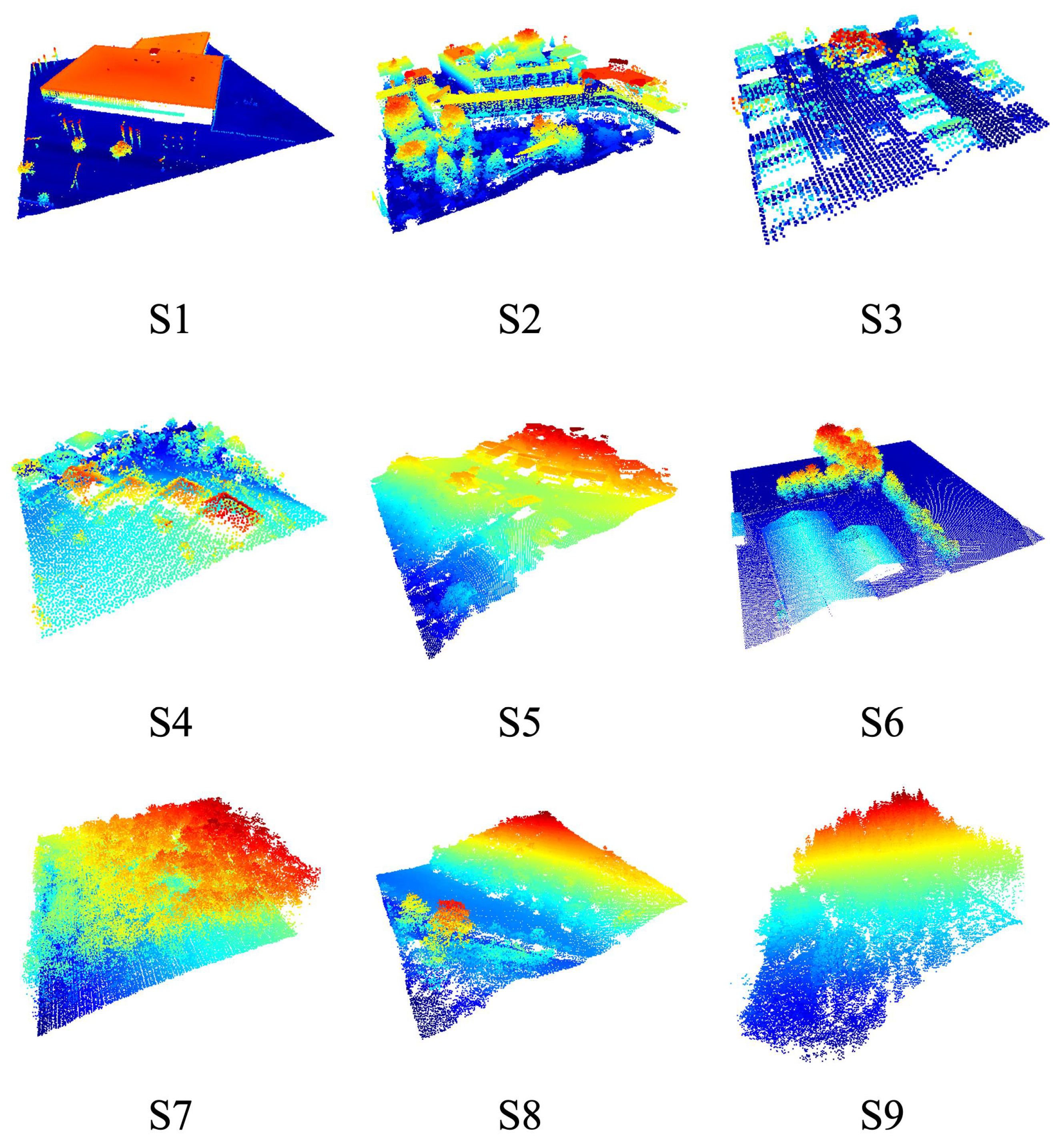
| Metropolis | Small City | Village | Mountain | |||||||
|---|---|---|---|---|---|---|---|---|---|---|
| S1 | S2 | S3 | S4 | S5 | S6 | S7 | S8 | S9 | Mean | |
| PointNet | 42.6 | 65.1 | 69.5 | 50.0 | 97.4 | 64.4 | 89.5 | 62.7 | 70.1 | 67.9 |
| PointNet++ | 77.9 | 76.5 | 98.7 | 93.6 | 100.0 | 92.5 | 100.0 | 78.7 | 82.4 | 88.9 |
| VoxelNeXt | 74.1 | 80.5 | 98.7 | 86.8 | 100.0 | 86.1 | 100.0 | 80.3 | 84.3 | 87.8 |
| BEV-MAE (Scratch) | 75.0 | 81.7 | 97.3 | 93.4 | 100.0 | 89.3 | 98.7 | 77.3 | 80.6 | 88.2 |
| BEV-MAE (Ours) | 77.8 | 81.2 | 97.3 | 90.8 | 100.0 | 90.4 | 100.0 | 81.6 | 85.2 | 89.4 |
| Method | mIoU (%) | OA (%) |
|---|---|---|
| PointNet++ [76] | 68.3 | 95.7 |
| KPConv [78] | 81.1 | 97.8 |
| RandLA [79] | 79.3 | 97.1 |
| EyeNet [80] | 79.6 | 97.2 |
| BEV-MAE (Scratch) | 77.9 | 97.3 |
| BEV-MAE (OpenGF [1]) | 77.3 | 97.2 |
| BEV-MAE (Random, 10 samples/project) | 77.6 | 97.3 |
| BEV-MAE (Random, 20 samples/project) | 77.8 | 97.2 |
| BEV-MAE (Random, 40 samples/project) | 77.7 | 97.3 |
| BEV-MAE (Ours, 10 samples/project) | 77.7 | 97.3 |
| BEV-MAE (Ours, 20 samples/project) | 78.0 | 97.3 |
| BEV-MAE (Ours, 40 samples/project) | 78.2 | 97.3 |
Disclaimer/Publisher’s Note: The statements, opinions and data contained in all publications are solely those of the individual author(s) and contributor(s) and not of MDPI and/or the editor(s). MDPI and/or the editor(s) disclaim responsibility for any injury to people or property resulting from any ideas, methods, instructions or products referred to in the content. |
© 2025 by the authors. Licensee MDPI, Basel, Switzerland. This article is an open access article distributed under the terms and conditions of the Creative Commons Attribution (CC BY) license (https://creativecommons.org/licenses/by/4.0/).
Share and Cite
Xiu, H.; Liu, X.; Kim, T.; Kim, K.-S. Advancing ALS Applications with Large-Scale Pre-Training: Framework, Dataset, and Downstream Assessment. Remote Sens. 2025, 17, 1859. https://doi.org/10.3390/rs17111859
Xiu H, Liu X, Kim T, Kim K-S. Advancing ALS Applications with Large-Scale Pre-Training: Framework, Dataset, and Downstream Assessment. Remote Sensing. 2025; 17(11):1859. https://doi.org/10.3390/rs17111859
Chicago/Turabian StyleXiu, Haoyi, Xin Liu, Taehoon Kim, and Kyoung-Sook Kim. 2025. "Advancing ALS Applications with Large-Scale Pre-Training: Framework, Dataset, and Downstream Assessment" Remote Sensing 17, no. 11: 1859. https://doi.org/10.3390/rs17111859
APA StyleXiu, H., Liu, X., Kim, T., & Kim, K.-S. (2025). Advancing ALS Applications with Large-Scale Pre-Training: Framework, Dataset, and Downstream Assessment. Remote Sensing, 17(11), 1859. https://doi.org/10.3390/rs17111859