


Sea Ice Concentration Manifestation in Radar Signal at Low Incidence Angles Depending on Wind Speed


Abstract

1. Introduction
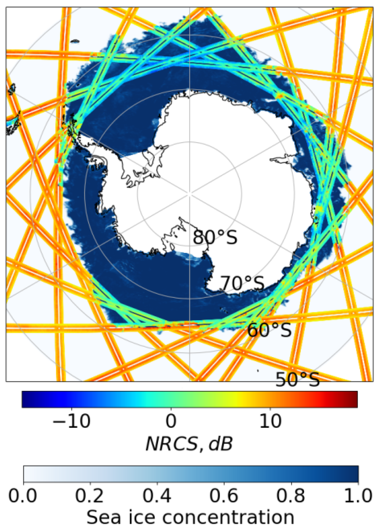
2. Data
3. Parameterization of NRCS Depending on Sea Ice Concentration and Wind Speed
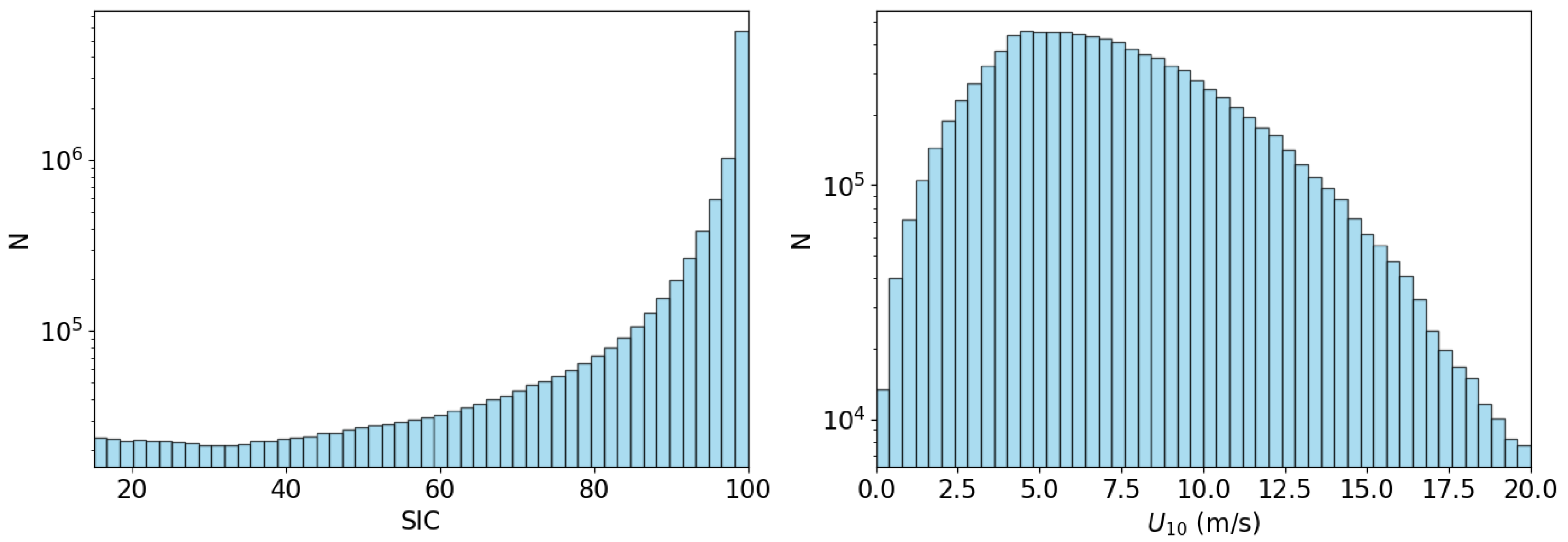
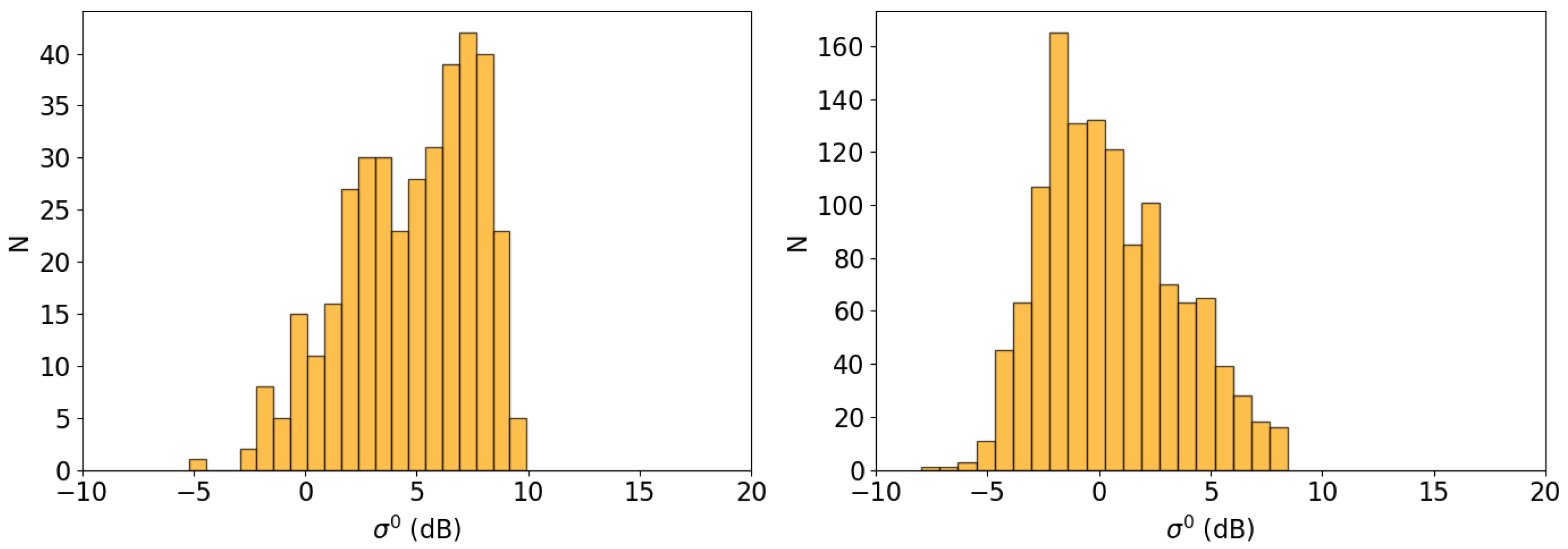
3.1. Binning Procedure
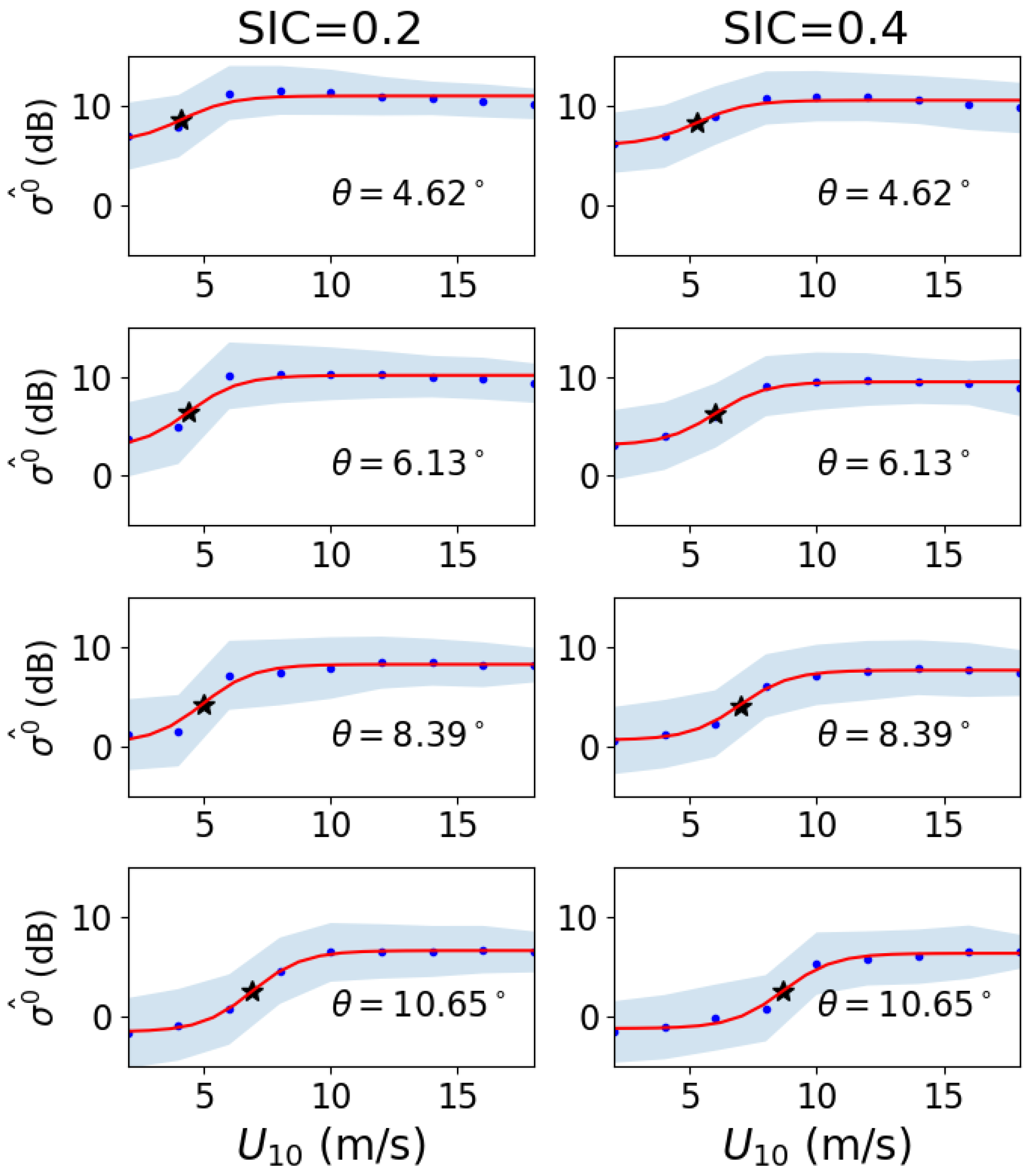
3.2. NRCS Dependence on Wind Speed and SIC
4. Results and Discussion
- The errors of mismatch of SIC and radar data: within one antenna footprint, various sea ice concentrations can be present;
- The sea ice concentration product is obtained from radiometer data, and the influence of the atmosphere may cause errors in defining this parameter;
- Wind speed is obtained from the reanalysis dataset, and these values may differ from real measurements; however, at this moment, reanalysis is the only source of information about wind speed over sea ice cover: remote sensing methods tuned for a water surface do not work there;
- Numerous factors regarding ice properties are not taken into account: the temperature of water and ice, the presence and conditions of snow cover, sea ice types, the size of sea ice floes [21], the relief of ice cover, ice thickness and salinity, etc.
5. Conclusions
Author Contributions
Funding
Data Availability Statement
Acknowledgments
Conflicts of Interest
Abbreviations
| AMSR-2 | Advanced Microwave Scanning Radiometer 2 |
| DPR | Dual-Frequency Precipitation Radar |
| GANAL | Japanese Global Analysis Model Data |
| GPM | Global Precipitation Measurements |
| NRCS | Normalized Radar Cross-Section |
| SIC | Sea Ice Concentration |
| SWIM | Sea Wave Investigation and Measurement |
| CFOSAT | Chinese–French Oceanic Satellite |
Appendix A

| Incidence Angle | a | b | c | d | e | f | g |
|---|---|---|---|---|---|---|---|
| 4.62° | 7.42 | 2.89 | 5.71 | 4.60 | 0.33 | 5.52 | 0.49 |
| 5.37° | 8.48 | 2.74 | 4.99 | 5.07 | −0.60 | 7.46 | 0.66 |
| 6.13° | 7.55 | 3.40 | 4.50 | 6.82 | −1.47 | 8.38 | 0.67 |
| 7.63° | 5.58 | 5.66 | 4.03 | 5.33 | −2.53 | 8.61 | 0.55 |
| 6.88° | 6.80 | 4.57 | 3.96 | 6.51 | −2.04 | 9.15 | 0.67 |
| 8.39° | 6.10 | 5.94 | 3.67 | 6.14 | −3.21 | 9.48 | 0.67 |
| 9.14° | 5.06 | 5.65 | 3.52 | 5.82 | −3.65 | 9.67 | 0.71 |
| 9.89° | 8.60 | 5.34 | 3.44 | 4.18 | −3.93 | 9.67 | 0.78 |
| 10.65° | 8.52 | 5.64 | 3.25 | 6.34 | −4.57 | 9.74 | 0.74 |
References
- Ivanova, N.; Johannessen, O.M.; Pedersen, L.T.; Tonboe, R.T. Retrieval of Arctic Sea Ice Parameters by Satellite Passive Microwave Sensors: A Comparison of Eleven Sea Ice Concentration Algorithms. IEEE Trans. Geosci. Remote Sens. 2014, 52, 7233–7246. [Google Scholar] [CrossRef]
- Spreen, G.; Kaleschke, L.; Heygster, G. Sea ice remote sensing using AMSR-E 89-GHz channels. J. Geophys. Res. Ocean. 2008, 113, 1–14. [Google Scholar] [CrossRef]
- Mäkynen, M.; Kern, S.; Tonboe, R. Evaluation of Microwave Radiometer Sea Ice Concentration Products over the Baltic Sea. Remote Sens. 2024, 16, 4430. [Google Scholar] [CrossRef]
- Naoki, K.; Ukita, J.; Nishio, F.; Nakayama, M.; Comiso, J.C.; Gasiewski, A. Thin sea ice thickness as inferred from passive microwave and in situ observations. J. Geophys. Res. Ocean. 2008, 113, C02S16. [Google Scholar] [CrossRef]
- Soriot, C.; Prigent, C.; Jimenez, C.; Frappart, F. Arctic Sea Ice Thickness Estimation From Passive Microwave Satellite Observations Between 1.4 and 36 GHz. Earth Space Sci. 2023, 10, e2022EA002542. [Google Scholar] [CrossRef]
- Lee, S.M.; Sohn, B.J.; Kim, S.J. Differentiating between first-year and multiyear sea ice in the Arctic using microwave-retrieved ice emissivities. J. Geophys. Res. Atmos. 2017, 122, 5097–5112. [Google Scholar] [CrossRef]
- Lindell, D.B.; Long, D.G. Multiyear Arctic Sea Ice Classification Using OSCAT and QuikSCAT. IEEE Trans. Geosci. Remote Sens. 2016, 54, 167–175. [Google Scholar] [CrossRef]
- Gao, X.; Pang, X.; Ji, Q. Sea ice classification in the Weddell Sea based on scatterometer data. Adv. Polar. Sci. 2017, 28, 196–203. [Google Scholar] [CrossRef]
- Laxon, S.; Peacock, N.; Smith, D. High interannual variability of sea ice thickness in the Arctic region. Nature 2003, 425, 947–950. [Google Scholar] [CrossRef]
- Pang, C.; Li, L.; Zhan, L.; Chen, H.; Shi, Y. Estimation of Arctic Sea Ice Thickness Using HY-2B Altimeter Data. Remote Sens. 2024, 16, 4565. [Google Scholar] [CrossRef]
- Horvat, C.; Buckley, E.; Stewart, M.; Yoosiri, P.; Wilhelmus, M.M. Linear Ice Fraction: Sea Ice Concentration Estimates from the ICESat-2 Laser Altimeter. EGUsphere 2023, 2023, 1–18. [Google Scholar] [CrossRef]
- Collard, F.; Marié, L.; Nouguier, F.; Kleinherenbrink, M.; Ehlers, F.; Ardhuin, F. Wind-Wave Attenuation in Arctic Sea Ice: A Discussion of Remote Sensing Capabilities. J. Geophys. Res. Ocean. 2022, 127, e2022JC018654. [Google Scholar] [CrossRef]
- Wadhams, P.; Squire, V.A.; Goodman, D.J.; Cowan, A.M.; Moore, S.C. The attenuation rates of ocean waves in the marginal ice zone. J. Geophys. Res. Ocean. 1988, 93, 6799–6818. [Google Scholar] [CrossRef]
- Huang, B.Q.; Li, X.M. Wave Attenuation by Sea Ice in the Arctic Marginal Ice Zone Observed by Spaceborne SAR. Geophys. Res. Lett. 2023, 50, e2023GL105059. [Google Scholar] [CrossRef]
- Panfilova, M.; Karaev, V. Sea Ice Detection by an Unsupervised Method Using Ku- and Ka-Band Radar Data at Low Incidence Angles: First Results. Remote Sens. 2023, 15, 3530. [Google Scholar] [CrossRef]
- Panfilova, M.; Karaev, V. Sea Ice Detection Method Using the Dependence of the Radar Cross-Section on the Incidence Angle. Remote Sens. 2024, 16, 859. [Google Scholar] [CrossRef]
- Chu, X.; He, Y.; Karaev, V.Y. Relationships Between Ku-Band Radar Backscatter and Integrated Wind and Wave Parameters at Low Incidence Angles. IEEE Trans. Geosci. Remote Sens. 2012, 50, 4599–4609. [Google Scholar] [CrossRef]
- Hauser, D.; Tourain, C.; Hermozo, L.; Alraddawi, D.; Aouf, L.; Chapron, B.; Dalphinet, A.; Delaye, L.; Dalila, M.; Dormy, E.; et al. New Observations From the SWIM Radar On-Board CFOSAT: Instrument Validation and Ocean Wave Measurement Assessment. IEEE Trans. Geosci. Remote Sens. 2021, 59, 5–26. [Google Scholar] [CrossRef]
- Ebuchi, N.; Graber, H.C. Directivity of wind vectors derived from the ERS-1/AMI scatterometer. J. Geophys. Res. Ocean. 1998, 103, 7787–7797. [Google Scholar] [CrossRef]
- Hossan, A.; Jones, W.L. Ku- and Ka-Band Ocean Surface Radar Backscatter Model Functions at Low-Incidence Angles Using Full-Swath GPM DPR Data. Remote Sens. 2021, 13, 1569. [Google Scholar] [CrossRef]
- Hwang, B.; Wilkinson, J.; Maksym, T.; Graber, H.C.; Schweiger, A.; Horvat, C.; Perovich, D.K.; Arntsen, A.E.; Stanton, T.P.; Ren, J.; et al. Winter-to-summer transition of Arctic sea ice breakup and floe size distribution in the Beaufort Sea. Elem. Sci. Anthr. 2017, 5, 40. [Google Scholar] [CrossRef]
- Stroeve, J.; Nandan, V.; Willatt, R.; Dadic, R.; Rostosky, P.; Gallagher, M.; Mallett, R.; Barrett, A.; Hendricks, S.; Tonboe, R.; et al. Rain on snow (ROS) understudied in sea ice remote sensing: A multi-sensor analysis of ROS during MOSAiC (Multidisciplinary drifting Observatory for the Study of Arctic Climate). Cryosphere 2022, 16, 4223–4250. [Google Scholar] [CrossRef]
- Alekseeva, T.; Tikhonov, V.; Frolov, S.; Repina, I.; Raev, M.; Sokolova, J.; Sharkov, E.; Afanasieva, E.; Serovetnikov, S. Comparison of Arctic Sea Ice Concentrations from the NASA Team, ASI, and VASIA2 Algorithms with Summer and Winter Ship Data. Remote Sens. 2019, 11, 2481. [Google Scholar] [CrossRef]
- Long, D.; Donelan, M.; Freilich, V.; Masuko, H.; Piersin, W.; Plant, W.; Weissman, D.; Wentz, F. Current Progress in Ku-band Model Functions; Technical Report MERS 96-002; Bringham Young University: Provo, UT, USA, 1996. [Google Scholar]
- Sergeev, D.A.; Kandaurov, A.A.; Troitskaya, Y.I. Investigation of the Pancake Ice Influence on the Wind–Wave Interaction Within Laboratory Modeling. In Conference the Physical and Mathematical Modeling of Earth and Environment Processes—2022; Karev, V.I., Ed.; Springer: Cham, Switzerland, 2023; pp. 257–261. [Google Scholar]
- Ban, W.; Zhang, L.; Zhang, X.; Nie, H.; Chen, X.; Chen, X. Wind-Concerned Sea Ice Detection and Concentration Retrieval From GNSS-R Data Using a Modified Convolutional Neural Network. IEEE J. Sel. Top. Appl. Earth Obs. Remote Sens. 2025, 18, 9755–9763. [Google Scholar] [CrossRef]
Disclaimer/Publisher’s Note: The statements, opinions and data contained in all publications are solely those of the individual author(s) and contributor(s) and not of MDPI and/or the editor(s). MDPI and/or the editor(s) disclaim responsibility for any injury to people or property resulting from any ideas, methods, instructions or products referred to in the content. |
© 2025 by the authors. Licensee MDPI, Basel, Switzerland. This article is an open access article distributed under the terms and conditions of the Creative Commons Attribution (CC BY) license (https://creativecommons.org/licenses/by/4.0/).
Share and Cite
Panfilova, M.; Karaev, V. Sea Ice Concentration Manifestation in Radar Signal at Low Incidence Angles Depending on Wind Speed. Remote Sens. 2025, 17, 1858. https://doi.org/10.3390/rs17111858
Panfilova M, Karaev V. Sea Ice Concentration Manifestation in Radar Signal at Low Incidence Angles Depending on Wind Speed. Remote Sensing. 2025; 17(11):1858. https://doi.org/10.3390/rs17111858
Chicago/Turabian StylePanfilova, Maria, and Vladimir Karaev. 2025. "Sea Ice Concentration Manifestation in Radar Signal at Low Incidence Angles Depending on Wind Speed" Remote Sensing 17, no. 11: 1858. https://doi.org/10.3390/rs17111858
APA StylePanfilova, M., & Karaev, V. (2025). Sea Ice Concentration Manifestation in Radar Signal at Low Incidence Angles Depending on Wind Speed. Remote Sensing, 17(11), 1858. https://doi.org/10.3390/rs17111858