Abstract
Weather forecasting is essential for agriculture, yet current methods often lack the localized accuracy required to manage extreme weather events and optimize irrigation. The MAGDA Horizon Europe/EUSPA project addresses this gap by developing a modular system that integrates novel European space-based, airborne, and ground-based technologies. Unlike conventional forecasting systems, MAGDA enables precise, field-level predictions through the integration of cutting-edge technologies: Meteodrones provide vertical atmospheric profiles where traditional data are sparse; GNSS-reflectometry offers real-time soil moisture insights; and all observations feed into convection-permitting models for accurate nowcasting of extreme events. By combining satellite data, GNSS, Meteodrones, and high-resolution meteorological models, MAGDA enhances agricultural and water management with precise, tailored forecasts. Climate change is intensifying extreme weather events such as heavy rainfall, hail, and droughts, threatening both crop yields and water resources. Improving forecast reliability requires better observational data to refine initial atmospheric conditions. Recent advancements in assimilating reflectivity and in situ observations into high-resolution NWMs show promise, particularly for convective weather. Experiments using Sentinel and GNSS-derived data have further improved severe weather prediction. MAGDA employs a high-resolution cloud-resolving model and integrates GNSS, radar, weather stations, and Meteodrones to provide comprehensive atmospheric insights. These enhanced forecasts support both irrigation management and extreme weather warnings, delivered through a Farm Management System to assist farmers. As climate change increases the frequency of floods and droughts, MAGDA’s integration of high-resolution, multi-source observational technologies, including GNSS-reflectometry and drone-based atmospheric profiling, is crucial for ensuring sustainable agriculture and efficient water resource management.
1. Introduction
Based on six international datasets, 2024 was confirmed by the World Meteorological Organization (WMO) as the warmest year on record. The global average surface temperature reached 1.55 °C above the 1850–1900 average [1]. The decade from 2015 to 2024 was the warmest on record, and climatic extremes have become increasingly frequent and intense.
Climate change is fundamentally reshaping agricultural systems by altering temperature regimes, precipitation patterns, and the availability of water resources [2]. Rising global temperatures have intensified evaporation rates, reduced soil moisture retention, and increased the frequency and severity of extreme weather events, such as heatwaves, droughts, and heavy precipitation. These changes pose significant risks to crop yields, irrigation practices, and food security, forcing the agricultural sector to adapt rapidly to evolving environmental conditions to tackle crop damage [3,4,5,6].
One of the most pressing challenges is precipitation variability, which has led to prolonged droughts in some regions and excessive rainfall in others. Southern Europe has experienced below-average rainfall, exacerbating drought conditions and increasing stress on water resources, while Northern Europe has faced above-average precipitation, leading to flooding, soil erosion, and reduced agricultural productivity.
Moreover, a crucial consequence of climate change is the decline in snow water volume, which impacts seasonal water availability for agriculture, as snow buffers winter precipitation into summer melt, when water demand peaks while precipitation declines [7,8,9]. These fluctuations create unstable growing conditions during the crop season, making it difficult for farmers to plan irrigation schedules and crop cycles effectively.
The Food and Agriculture Organization (FAO) of the United Nations reports that around 70% of global water use is attributed to agriculture. Furthermore, by 2030, irrigation water withdrawal is expected to grow by about 14%, according to the FAO irrigated area forecast [10]. This highlights the growing importance of optimizing irrigation water usage in addressing the challenges of increasing water scarcity [11].
The unpredictability of water availability due to climate variability increases the demand for advanced decision-support tools to optimize water distribution and minimize waste. Recent projections indicate that climate change could lead to yield reductions of up to 22% for grain maize in Europe, with Southern regions being particularly affected [12]. Wheat yields in Southern Europe are expected to decrease by up to 49%, while Northern Europe may experience some compensatory benefits from increasing atmospheric CO2 levels and altered precipitation regimes [12]. Adaptation measures such as crop variety changes, enhanced irrigation techniques, and soil management could mitigate losses, but sustainable water limits may restrict large-scale expansion. Additionally, extreme weather events, including heatwaves and heavy rainfall, could impact both crop yields and soil conditions, posing further challenges for farmers [12,13,14].
Modern technologies have significantly improved irrigation water management over recent decades, addressing water scarcity challenges through mechanical, electrical, and software advancements [15,16]. These innovations enable precise control over water distribution and support optimized allocation at larger scales.
Irrigation scheduling determines the optimal timing and volume of water application. Over the past two decades, various Decision Support Systems for Irrigation Scheduling (IS-DSS) have been developed to assist farmers and managers [17,18,19]. These systems integrate Earth Observation (EO) techniques for crop monitoring [20,21,22,23,24], weather forecasts [25,26,27,28,29,30], soil water balance models [31,32], and machine learning [15,16,33], offering a combined approach to efficient irrigation planning. Each of these methodologies presents specific advantages and limitations, requiring a combined approach to maximize efficiency in irrigation planning, as demonstrated in the MOSES project [34], and highlighting the need for systems that can more accurately forecast high-impact weather events affecting crops [35,36,37].
In this context, the MAGDA (Meteorological Assimilation from Galileo and Drones for Agriculture) project delivers a highly innovative approach to precision irrigation, addressing key challenges in climate-resilient agriculture. By integrating real-time atmospheric data from GNSS signals, drone-based meteorological profiling, Copernicus Earth Observation data, ground-based radar, and in situ sensors, MAGDA creates a dynamic, data-driven framework for weather and irrigation forecasting. The system significantly improves short- and very short-term predictions, enabling farm-specific adaptive water management strategies. Using cost-efficient GNSS stations and Meteodrones for high-resolution atmospheric profiling, MAGDA overcomes limitations of defining initial conditions for numerical weather prediction models and contributes to enhancing weather forecasts. Its irrigation advisory service integrates the SPHY hydrological model, offering accurate water balance simulations, while severe weather forecasts are generated using high-resolution numerical weather prediction models assimilating various types of observations. Furthermore, MAGDA delivers its insights through developer-friendly APIs for seamless integration into Farm Management Systems, making advanced, hyper-local weather and irrigation data accessible and actionable for end-users. Through this combination of multi-source data assimilation, predictive modeling, and user-oriented services, MAGDA provides a novel, operational solution that enhances resilience and efficiency in agricultural water management. It represents a step forward for precision irrigation by combining high-resolution, multi-source datasets, real-time monitoring, and predictive analytics, ensuring sustainable agricultural water management and improved extreme weather forecasting under climate change conditions.
This paper is structured as follows: Section 2 describes the materials and methods, MAGDA demonstrator sites, and the advanced observation technologies deployed, including GNSS, Meteodrones, in situ sensors, and satellite data. It also outlines the forecasting models, the integration of MAGDA services into Farm Management Systems, and the validation methods used for meteorological and hydrological assessments. Section 3 presents the results, followed by a discussion in Section 4 and final conclusions in Section 5.
2. Materials and Methods
2.1. MAGDA Demonstrator Sites
The MAGDA project is being tested across three demonstrator sites strategically selected in different agricultural regions of Europe. These sites, located in Italy, France, and Romania, encompass diverse climatic conditions, soil types, and crop types, allowing for the evaluation of MAGDA’s integrated system in a variety of agricultural contexts (Figure 1). Each site is characterized by distinct crop water requirements, irrigation methods, and vulnerability to climate variability, providing a comprehensive assessment of MAGDA’s flexibility and performance.

Figure 1.
MAGDA project sites location and crop types with an example of the deployed sensors.
2.1.1. Italy–Fruit Orchards
The first demonstrator site is situated in the Cuneo province, in the Piedmont region of northern Italy, one of the most significant fruit-producing areas in the country. The region specializes in the cultivation of apples, peaches, kiwis, plums, cherries, almonds, and hazelnuts. Farmers in this area rely on both natural rainfall and irrigation systems, which vary from traditional drip irrigation to more advanced precision techniques.
The primary objective at this site is to improve short-term rainfall forecasting and optimize water resource management for fruit orchards. The MAGDA system integrates GNSS receivers, Meteodrones, and in situ sensors to measure soil moisture, atmospheric water vapor, temperature, and precipitation. This information helps farmers make data-driven irrigation decisions, reducing water waste while ensuring optimal conditions for crop growth.
Several farms within a 4.5–7 km radius have been equipped with MAGDA sensors, strategically positioned to monitor microclimatic variations. These data points are also used for assimilation into weather models, particularly for forecasting localized thunderstorms and hail events, which represent a major risk factor for fruit production.
2.1.2. France–Vineyards
The second demonstrator site is located in Burgundy, France, particularly in the Beaune Valley, a globally renowned wine-producing region. The test site includes vineyards owned by Maison Louis Jadot, a prestigious winery producing high-quality wines. Burgundy’s vineyards are highly sensitive to temperature fluctuations, frost events, drought stress, and extreme rainfall, all of which can impact grape quality and yield.
MAGDA’s deployment in Burgundy focuses on climate adaptation for viticulture, using an array of GNSS sensors, Meteodrones, and in situ weather monitoring stations installed across different vineyard locations. These sensors track air and soil temperature, humidity, wind speed, and solar radiation, helping viticulturists anticipate weather-related risks and optimize vineyard management strategies.
MAGDA’s implementation in Burgundy is designed to enhance extreme weather anticipation, particularly for convective storms and hail events, although the countermeasures currently available to vineyard managers remain only partially effective. Among the strategies currently in use at Maison Louis Jadot and its network of vineyard growers are field candles and heating wires for late frost, as well as chimney networks for hail protection.
Another key priority for stakeholders is improving the usability of meteorological data for decision-making. While growers currently rely on an existing forecasting portal, they find the data difficult to interpret and not always reliable. There is strong interest in more actionable and accessible weather insights, which aligns closely with MAGDA’s interoperability and dashboard tasks.
Although vineyards in Burgundy do not require irrigation infrastructure, there is a strong demand for better water status monitoring at the vineyard level. Understanding soil moisture conditions can inform adaptive soil management practices, helping growers optimize grape production. The transition from macro-level weather insights to localized, field-specific data is a critical step in improving climate resilience in viticulture, and MAGDA’s sensor network is designed to support this shift.
2.1.3. Romania–Cereal and Oilseed Farming
The third demonstrator site is located in Brăila County, Romania, within the Danube River floodplain and the Bărăgan Plain, which is the most fertile agricultural area in Eastern Europe. This region supports large-scale industrial farming of summer crops, including corn, sunflower, soybean, wheat, and barley. Farmers in Brăila face significant challenges related to water availability, soil moisture variability, and extreme weather events such as droughts and floods.
The MAGDA test site in Brăila consists of three sensor deployment areas: one within the Embanked Great Island of the Danube River and two further inland in the Bărăgan Plain. These locations have been selected to assess spatial variability in soil moisture and crop water requirements.
MAGDA’s real-time data assimilation system aims to improve irrigation planning by integrating satellite-derived soil moisture data, in situ GNSS reflections, and atmospheric observations from Meteodrones. By correlating historical precipitation data with current field conditions, the system helps agricultural stakeholders optimize their irrigation schedules and prepare for extreme weather events, ensuring better crop resilience and resource efficiency.
2.2. Data-Collecting Sensors Used in the Project: GNSS, Meteodrones, In Situ Sensors, Sentinel
The observation system developed within the MAGDA project integrates GNSS receivers, Meteodrones, in situ meteorological and soil sensors, and Copernicus Sentinel satellite data, forming a multi-platform, high-resolution monitoring network. This system is designed to improve the accuracy of numerical weather prediction (NWP) models and hydrological simulations by providing continuous, multi-source observational data.
In addition to leveraging pre-existing observation networks—including weather radars, meteorological stations, and permanent GNSS networks—MAGDA has deployed new observational assets directly within agricultural fields of interest. The installation of low-cost GNSS receivers, Meteodrones, and in situ metIS sensor hubs enables localized, high-resolution environmental monitoring, improving the characterization of key meteorological and hydrological variables. The newly deployed sensors are integrated with existing data sources through dedicated assimilation and processing frameworks, ensuring a synergistic use of satellite, airborne, and ground-based observations.
2.2.1. Gnss-Based Atmospheric and Soil Moisture Observations
GNSS data are used to retrieve tropospheric delay parameters for atmospheric water vapor estimation, as well as soil moisture content via GNSS-Reflectometry (GNSS-R). The MAGDA project utilizes a combination of permanent GNSS networks—such as the European Permanent Network (EPN)—and newly installed GNSS receivers at agricultural demonstration sites to provide high-resolution data.
The primary meteorological parameter derived from GNSS is Zenith Total Delay (ZTD), computed using Precise Point Positioning (PPP) algorithms [38], which represent the total atmospheric delay experienced by GNSS signals due to refraction by water vapor and dry air. In the MAGDA project, ZTD is assimilated into the WRF model (WRFDA), where it helps improve short-term weather forecasts by refining atmospheric moisture fields [39]. The assimilation of ZTD allows for a direct constraint on atmospheric humidity, reducing errors in water vapor estimation and improving forecast skill, particularly in convective events.
For soil moisture estimation, GNSS-R techniques analyze signal-to-noise ratio (SNR) interference patterns from dual-frequency GNSS receivers, enabling the retrieval of surface soil moisture variability [40]. The integration of GNSS-R soil moisture retrievals with Sentinel-derived soil moisture products and in situ soil sensors provides a multi-source validation framework for hydrological modeling.
2.2.2. Meteodrones for High-Resolution Vertical Profiling
Meteodrones were strategically deployed in agricultural regions to complement radiosonde observations and ground-based meteorological station networks, offering high-resolution vertical atmospheric profiling. The Meteodrone MM-670 is equipped with high-precision sensors for temperature, relative humidity, and pressure. Wind speed and direction are computed from the attitude of the Meteodrone. Meteodrones can operate in wind speeds of up to 90 km/h, withstand moderate rain, and fly through fog and clouds under icing conditions thanks to their integrated de-icing system.
The Meteodrones are pre-programmed to perform a straight vertical ascent/descent at a constant climb rate of 10 m/s up to a maximum altitude of 6000 m (AMSL). A typical flight profile takes 22 min. However, custom flights are also possible. The flights are controlled by an onboard autopilot system. The flights in Italy were conducted on-site by a pilot using a mobile drone system, while the flights in France and Romania were operated remotely from Meteomatics’ headquarters in St. Gallen, Switzerland, using a Meteobase. The Meteobase serves as a ground station for remote Meteodrone operations, enabling the automated launch and landing of Meteodrones.
Meteodrone flights were conducted at all demonstration sites (Italy, France, and Romania), providing detailed vertical profiles of atmospheric stability, boundary layer processes, and moisture transport. The collected data were integrated into WRF simulations, ensuring a coherent assimilation strategy alongside GNSS-ZTD and in situ temperature/humidity data.
2.2.3. In Situ Meteorological and Soil Sensors
The MAGDA project deployed metIS hubs as part of its in situ sensor network to enhance localized environmental monitoring in agricultural areas. These hubs were specifically designed to provide high-frequency meteorological and soil measurements and were deployed across the demonstration sites. The metIS hubs integrate various sensor configurations, including air temperature and humidity sensors, anemometers, rain gauges, soil moisture probes, and leaf wetness sensors, making them a versatile solution for both meteorological and agronomic monitoring.
The hubs were deployed in two configurations: as standard weather stations, and as in-crop sensors placed directly within cultivated fields to provide more representative environmental data. The weather station configuration included wind speed, rainfall, air temperature, humidity, and soil temperature and moisture sensors, while the in-crop configuration focused on leaf wetness duration and soil properties relevant to precision agriculture.
Data from the metIS hubs were transmitted every 15 min via cellular networks, initially using 2G connectivity, which was later upgraded to LTE-M to improve data transmission reliability, particularly in rural areas where network coverage was initially problematic. These data were processed and stored in the CAP 2020 infrastructure and made accessible to the MAGDA forecasting system through a structured API, ensuring seamless integration with numerical weather prediction (NWP) and hydrological models.
The validation of the metIS hub measurements was conducted by comparing their outputs with data from existing meteorological station networks, Sentinel satellite observations, and GNSS-Reflectometry (GNSS-R) soil moisture retrievals. This multi-source validation framework ensured that the hubs provided accurate and reliable environmental data, thus enhancing the representation of small-scale meteorological and soil moisture variations essential for agricultural decision-making.
The modular and easy-to-deploy nature of the metIS hubs allowed MAGDA project partners to install them efficiently across different demonstration sites, reducing setup costs while significantly enhancing localized meteorological monitoring capabilities. Their integration into the broader observation network, alongside GNSS, Meteodrones, and Sentinel, further strengthened the multi-scale, high-resolution monitoring strategy adopted within the project, providing valuable input for improved weather forecasting, hydrological modeling, and agricultural risk assessment.
2.2.4. Copernicus Sentinel Earth Observation Data
The Copernicus Sentinel satellite constellation, developed by the European Space Agency (ESA), provides high-resolution Earth observation data that are critical to environmental monitoring, land surface characterization, and hydrological modeling. The MAGDA project integrates data from Sentinel-1, Sentinel-2, and Sentinel-3, leveraging their complementary capabilities to retrieve key parameters such as soil moisture, land cover, vegetation indices, and land surface temperature (LST).
Sentinel-1, a synthetic aperture radar (SAR) mission, is particularly valuable for all-weather soil moisture estimation. Unlike optical sensors, SAR data acquisition is unaffected by cloud cover and sunlight availability, making it suitable for continuous soil moisture monitoring. Within the MAGDA framework, Sentinel-1 backscatter coefficients are processed to derive surface soil moisture variability, complementing GNSS-Reflectometry (GNSS-R) and in situ soil moisture sensors. The integration of Sentinel-1 data enables frequent and high-resolution monitoring of soil moisture conditions, which is critical for hydrological applications.
Sentinel-2, a multi-spectral imaging mission, provides high-resolution optical data for vegetation monitoring, agricultural land use classification, and water stress assessment. The project utilizes the Normalized Difference Vegetation Index (NDVI) and the Moisture Stress Index (MSI) to evaluate crop health and irrigation needs. NDVI is calculated using the near-infrared (NIR) and red spectral bands to assess vegetation vigor, with values ranging from −1 (water bodies) to 1 (dense vegetation). The MSI, derived from the shortwave infrared (SWIR) and NIR bands, provides a quantitative estimate of vegetation moisture stress, where higher values indicate greater water stress. These vegetation indices are processed at 10 m spatial resolution and analyzed for the period from 2015 to the present, ensuring a long-term perspective on crop conditions.
Sentinel-3, specifically its Sea and Land Surface Temperature Radiometer (SLSTR), provides Land Surface Temperature (LST) products at a 1 km resolution with a daily frequency of four observations (two from Sentinel-3A and two from Sentinel-3B). LST is a critical variable for evapotranspiration (ET) estimation, an essential component of the agricultural water balance and drought assessment. The MAGDA project processes actual evapotranspiration using the Sen-ET SNAP plugin, developed by EOatDHI (Hørsholm, Denmark) in the Sen-ET project (https://www.esa-sen4et.org/) and financed by ESA. It is a model based on the Two-Source Energy Balance (TSEB) approach [41]. This methodology integrates solar radiation flux, latent heat flux, and atmospheric parameters to compute actual evapotranspiration (ETdaily), which is crucial for precision irrigation and water resource management.
The integration of Sentinel-derived products with in situ observations and numerical weather prediction (NWP) models ensures that remote sensing datasets are properly validated and assimilated. The Sentinel datasets were assessed for temporal and spatial alignment with key weather events, ensuring that their outputs could be effectively incorporated into MAGDA’s forecasting and hydrological modeling framework. However, the feasibility of operational integration is influenced by satellite revisit times, particularly for real-time monitoring of fast-developing weather phenomena. This limitation is addressed through continuous in situ monitoring of soil moisture, which offers high temporal resolution. By integrating Sentinel-derived products with in situ data, it is possible to bridge the spatial and temporal gaps inherent to each monitoring approach, thereby enhancing high-resolution environmental analysis within MAGDA.
2.3. Forecasting Models
2.3.1. Meteorological Model Setup
The meteorological model used in the MAGDA project is based on the Weather Research and Forecasting (WRF) system [42], configured to simulate atmospheric conditions over the selected study areas. The model was implemented with two domain configurations: one covering Italy and France, and the other focused on Romania. Each configuration consists of three nested domains with spatial resolutions of 22.5 km, 7.5 km, and 2.5 km (Figure 2A,B).
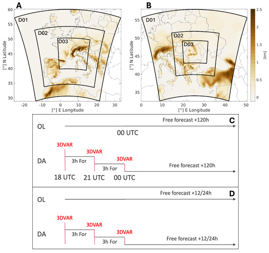
Figure 2.
MAGDA domain configuration and data assimilation setup. (A) shows the three nested WRF domains used for the Italian and French demonstrator sites, and (B) for the Romanian site. The outermost domain (D01) covers approximately 30–60°N and 20°W–30°E in (A), and 30–60°N and 0–50°E in (B), with a horizontal resolution of 22.5 km. The intermediate domain (D02) spans roughly 35–55°N and 10–20°E in (A), and 35–55°N and 10–40°E in (B), at 7.5 km resolution. The innermost domain (D03) focuses on the pilot areas, ranging from approximately 39°N to 50°N and 0° to 15°E in (A), and from 42°N to 48°N and 20°E to 30°E in (B), with 2.5 km resolution. Latitude and longitude tick labels are shown for both panels. (C) illustrates the forecast configuration for hydrological and irrigation applications, where 3DVAR assimilation is applied at 18:00, 21:00, and 00:00 UTC, followed by a 120-h free forecast starting at 00:00 UTC. (D) presents the rapid-update scheme adopted for convective storm forecasting, involving 3-hourly 3DVAR cycles and a 12–24-h forecast horizon to enhance short-term storm prediction.
The model employs physical parameterization schemes validated in prior studies on similar meteorological events [39,43,44,45,46]. The schemes adopted for the WRF-OL (Open Loop, without assimilation) and WRF-DA (Data Assimilation) simulations include the WSM6 microphysics scheme [47], the YSU planetary boundary layer scheme [48], the RRTMG longwave and shortwave radiation schemes [49], and the RUC land surface model [50]. Cumulus parameterization is explicitly applied in the innermost domain (D03). These parameterizations were selected for their ability to accurately reproduce the regional meteorological conditions relevant to the project. The YSU scheme ensures a realistic representation of vertical mixing, while the WSM6 scheme simulates mixed-phase cloud processes, thereby improving precipitation forecasts.
Data assimilation was performed using a three-dimensional variational (3DVAR) approach available in WRFDA [51], incorporating an outer-loop procedure [52]. This iterative process updates the analysis field, allowing previously rejected observations to be assimilated in subsequent cycles. The number of outer loops was determined via sensitivity tests on selected use cases balancing computational cost and the number of assimilated observations. Three outer loops were found to offer an optimal trade-off, significantly improving the analysis while maintaining reasonable computational demand. This setup is consistent with CIMA’s operational meteorological forecasting chains, including those used for nowcasting [53,54], and ensures progressive refinement of the background field through each assimilation cycle.
The background error covariance matrix (B matrix) was computed using the NMC method [55], applied to July 2020 forecasts with 24-h and 12-h lead times at 00:00 UTC. Differences between t + 24 and t + 12 forecasts for the same initialization time were used to derive domain-specific error statistics, enabling seasonally adjusted background error estimates for each simulation period.
Two forecasting strategies were implemented to support hydrological and convective storm applications. For hydrological and irrigation use cases, a 120-h (5-day) forecast is initialized daily at 00:00 UTC, assimilating observations at 18:00, 21:00, and 00:00 UTC (Figure 2C). The impact of assimilation is primarily evaluated within the first 24 h, while the full forecast provides input to the hydrological model. For convective storm nowcasting, a rapid-update cycle was adopted, featuring a 3-hourly 3DVAR assimilation and a 12-h forecast horizon (Figure 2D).
The main objective of the MAGDA project was to design a forecasting chain with a high degree of operational readiness by the end of the project. For this reason, the configuration of the assimilation cycles was not exploratory, but instead built upon a robust foundation of prior research, consolidated over time through multiple peer-reviewed publications, applications across various contexts, and several years of experience in operational forecasting environments [39,45,46,53,54,56,57,58,59,60].
2.3.2. Agrohydrological Model Setup
The irrigation advisory service of MAGDA rests on the SPHY model [61], whose irrigation module has been improved and adapted for delivering short-term and mid-term forecasts (up to 5 days ahead) of Irrigation Water Requirements (Figure 3).
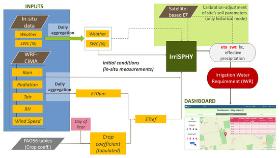
Figure 3.
Flowchart of the MAGDA irrigation advisory service.
Irrigation Water Requirement (IWR) is defined here as the supplemental water needed to meet crop water demand that is not fulfilled by rainfall and existing soil moisture. IWR is computed as:
where ETc is the crop reference evapotranspiration under non-stress conditions, and Etc,act is the actual crop evapotranspiration. Peff is the effective precipitation, and ETsm is the fraction of the soil water content at the root-zone that is taken by crops for evapotranspiration (also known as the Root Zone Water Supply). The component is the total of water available from rainfall and soil moisture that is used at each timestep to meet the crop water requirement. Under stress conditions for which rainfall and soil moisture stored in the root-zone () do not match the crop water requirements (ETc), the component may be similar to the crop evapotranspiration computed by using satellite-based evapotranspiration methods.
Conceptually, the SPHY model used in MAGDA adopts a simplified 1D leaky-bucket approach, which simulates the dynamics of soil water content in the root-zone domain by considering the main inflows (rainfall) and outflows (interception, actual evapotranspiration, and drainage) that account in the soil–crop–atmosphere continuum (Figure 4A).
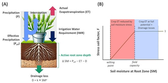
Figure 4.
Conceptual flowchart of the MAGDA irrigation advisory service: (A) Main inflow and outflow fluxes simulated in the root-zone domain, (B) Subdomains of flux simulation based on the actual soil moisture content in the root-zone and the soil moisture at the wilting point and field capacity.
The water balance in the root-zone domain is computed as:
being SM the soil moisture in the root zone in water depth, Inf is the fraction of the rainfall that infiltrates into the root zone after canopy interception is discounted, D is the volume of water outflowing the root zone due to vertical or lateral drainage, and ET is the actual evapotranspiration.
Drainage is computed using a power–law relationship:
where EWC (mm/day) refers to the Excess Water Content or amount of water that exceeds the soil’s field capacity after accounting for precipitation inflows within the root zone (saturation-excess approach). Parameters k and p define the soil drainable-water retention curve of a soil, with k being the diffusivity coefficient (mm2/day) and p the moisture diffusivity exponent (dimensionless). The impact of different values in p and k controls how drainable water is retained in the root zone, and therefore the intrinsic capacity of the soil to buffer the onset of plant water stress and hence the need for irrigation. Both parameters can be empirically calibrated from the decay of the soil moisture observed in the root zone profile immediately after rainfall events, when drainage may account for this and evapotranspiration losses are minimal. When soil moisture data is not available, typical values from literature can be adopted. Although the impact of different k-p paired values may have a critical impact on the generation of drainage and the onset of dryness conditions, this effect can be abruptly reduced when conditions for the generation of drainage are not met. Conditions for drainage generation in our analysis were only met in 2% of all the simulation runs due to the combination of (a) initial conditions with very dry soils very far from the field capacity), (b) small-size rainfall events (less than 25 mm) that were not enough for reaching the field capacity of the soils, and (c) an irrigation strategy which aims to meet crop water requirements at each timestep instead of filling the soil bucket up to the field capacity. Due to the difficulties found in calibrating the k-p parameters and considering the boundary conditions of our study, typical values of 0.2 for k and 1.5 for p were adopted.
Actual evapotranspiration from the root-zone domain ( in Equation (1)) is estimated using the FAO56 algorithm [62] and incorporates a stress factor () when soil moisture levels fall between the wilting point (wp) and field capacity (fc) (Figure 4B). ranges from 0, when soil moisture is lower than the wilting point, to 1 when soil moisture exceeds the field capacity. Both soil parameters, wp and fc, can be set up based on laboratory analyses or derived from pedotransfer functions if data on soil texture and organic matter content are known.
is crop reference evapotranspiration computed according to the Penman–Monteith–FAO equation [63]. is the crop coefficient under optimal or non-stress conditions.
In this study, SPHY was set up and tested in the SCDAB and Tetto-Bernardo pilot sites, assuming the general parameters listed in (Table 1)). For Kc values, the 4-stage growth model suggested by the FAO Irrigation and Drainage Paper No. 24 [64] was adopted. In both pilot sites, the crop season was split into initial, development, middle, and end stages; each one characterized by a particular length and a tabulated or expert-based crop coefficient Kc (see (Table 2)). The starting and ending dates for each stage of the crop were calculated once the planting date was fixed.

Table 1.
Site parameters used in the irrigation advisory service.
Table 2.
Duration of crop development stages and crop coefficients for maize-grain (SCDAB) and apple (Tetto-Bernardo) crops.
2.3.3. Weather Forcings and Forecasting Windows
The SPHY model was forced using weather forecasts generated with and without assimilation. Forecasts without data assimilation (OL) do not include MAGDA system data from in situ sensors, GNSS, and/or Meteodrones. This configuration is considered in this study as the benchmark for comparison purposes. DA forecasts assimilate diverse data sources, depending on availability: radar data, GNSS data, in situ temperature measurements, and data retrieved from Meteodrones.
The impact of assimilation is expected to be more relevant during the first 12 to 24 h after the assimilation of in situ data, and progressively decreases as the forecast window extends. The magnitude of this impact may vary across test cases, depending on factors such as the quantity and type of observations available, atmospheric conditions at assimilation time, and event typology. Differences in IWR forecasts between OL and DA products highlight the potential advantages of using data assimilation in terms of water savings and more accurate irrigation quota adjustments.
To account for spatial variability and uncertainty in weather forecasts, SPHY was forced with an ensemble of 49 forecast paired-value vectors of precipitation and reference evapotranspiration. Each member represents forecast trajectories generated within a bounding box of 21 km × 21 km area (7 × 7 grid points in the forecast mesh). The final recommendation of irrigation at each pilot site is delivered as the mean value of all IWR figures simulated in the ensemble.
The demonstrator was run on the SCDAB (Romania) Tetto-Bernardo (Italy) pilot sites during different testing periods throughout the summer and autumn of 2024. In selecting the dates, priority was given to the occurrence of rainfall events and to periods with the highest availability of MAGDA data from GNSS, Meteodrone flights, and/or field-scale weather and soil moisture sensors. The final selected dates are reported in Table 3. In order to comply with the user requirements previously surveyed among farmers and stakeholders, IWR forecasts were generated/updated with a frequency of 2 days, starting in our analysis from the beginning of each testing period. For comparison purposes between OL and DA, and short-term and medium-term forecast outcomes, results in Section 3 are delivered as the average of all the IWR retrieved in a common period of 5–6 days.
Table 3.
Forecasting time windows tested per pilot site and total rainfall measured.
2.4. Farm Management System Integration
Farm Management Systems (FMS) represent a technological evolution in agriculture, providing farmers with advanced tools to optimize the management of their farms. These systems integrate agro-meteorological data, soil and crop information, and predictive models to guide agronomic decisions in real time.
The benefits are substantial: increased production efficiency, reduced operational costs, and minimized environmental impact through targeted use of resources such as water and agrochemicals. Moreover, FMS can enhance product traceability and quality, two aspects that are increasingly demanded by environmentally and socially conscious consumers.
2.4.1. A Variety of End Users
Potential end users of MAGDA outputs vary significantly across the different demonstration sites and regions of Europe. From the small clos in Burgundy to the large agricultural fields in Romania, there is a common interest in enhanced extreme weather forecasts and decision-supporting data.
End users include not only farmers but also agricultural advisors, operating at various scales. The demonstration sites also host a variety of crops: vineyards in France and orchards in Italy, which are perennial crops, and cereals in Romania.
The impacts of extreme events differ between perennial and annual crops. For instance, frost or hail can affect both the current and subsequent year’s yields in vineyards and orchards, while extreme heat can result in permanent damage to trees and vines. Hydric stress primarily affects orchards and cereals, where precise irrigation recommendations based on reliable forecasts can significantly improve water management practices.
This context led MAGDA’s partners to develop both an API and a dashboard to provide access to the data collected and generated by the system, paving the way for seamless integration into Farm Management Systems.
2.4.2. The Challenging Task of FMS Interoperability
The integration of data generated by the infrastructure developed during this project, which includes meteorological and agro-meteorological information to enhance crop management, poses significant challenges when attempting to interface with third-party systems such as Farm Management Systems (FMS). These challenges stem primarily from the proprietary nature of these systems, which often require custom development efforts by their publishers to enable compatibility with external data sources.
However, these publishers are typically reluctant to invest in such developments unless there is substantial demand and pressure from their user base. This creates a bottleneck for the adoption of innovative data-driven solutions in agricultural management, as the value of integrating these new data streams is often not immediately recognized or prioritized by the FMS providers.
To address this issue and ensure the usability of the project’s outputs across diverse systems, we adopted an open API (Application Programming Interface) approach. By providing an open API, the results and insights generated through the project can be made accessible to any third-party system willing to integrate them, without requiring proprietary developments from the FMS providers themselves.
This approach not only removes the dependency on specific publishers but also empowers end users and stakeholders to leverage the data in ways that suit their unique requirements.
The dashboard itself is designed to meet the need for accessible, actionable data from the MAGDA infrastructure. It also uses MAGDA’s API and demonstrates the interest of MAGDA to the end user, using visualizations for both raw in situ sensor data and model outputs.
Dashboard components can also be embedded within third-party systems, such as graphs integrated into extranets, thus facilitating interoperability and wider adoption.
2.4.3. Functionalities of the Dashboard
We aimed to provide a simple yet powerful dashboard, capable of displaying data from MAGDA’s infrastructure in a comprehensive and user-friendly way (Table A1). The dashboard was made accessible to MAGDA’s stakeholders throughout the entire project via four successive versions, each incorporating additional features.
Initial feature prioritization was based on interviews with key users and resulted in a first version offering basic data visualization, alert functions, and the ability to group sensors into specialized categories. During the project, field demonstrations of the dashboard (in France, Italy, and Romania) were conducted to collect feedback and fine-tune specific functionalities, including enhanced display customization for different user needs.
An additional objective was to ensure that the dashboard could highlight the differences between forecasts produced with and without assimilation of MAGDA sensor data. This was particularly useful for demonstration purposes during selected extreme weather events captured throughout the operational phase of the project.
2.5. Validation Methods
2.5.1. Meteorological Validation
The meteorological validation of the WRF model in the MAGDA project was conducted using the MODE (Method for Object-Based Diagnostic Evaluation) technique, an object-oriented verification method designed to assess spatial agreement between forecasted and observed precipitation fields. This approach provides diagnostic insights that are more directly interpretable than traditional grid-point verification techniques, making it particularly useful for evaluating high-resolution numerical weather prediction (NWP) models [65,66,67].
MODE identifies precipitation objects in both forecast and observation fields, characterizing their attributes such as area, centroid position, orientation, intersection, and intensity ratio [68]. Key spatial attributes include rainfall extent characteristics such as area ratio and intersection area, and spatial relationships such as centroid distance and angle difference. These descriptors quantify the shape, orientation, and spatial alignment of forecasted versus observed features. The primary statistical indices used for evaluation were the Frequency Bias Index (FBIAS), the Probability of Detection (POD), the Critical Success Index (CSI), and the False Alarm Rate (FAR) [67].
The assimilation analysis of 2mT, ZTD, and reflectivity was summarized using a boxplot approach to assess improvements at each assimilation cycle across different variables. Boxplots provide a visual representation of the distribution of bias and standard deviation, offering a statistical summary to evaluate how assimilation impacts model accuracy by examining changes in central tendency, variability, and outliers. The boxplot includes the first quartile (Q1), third quartile (Q3), and interquartile range (IQR = Q3 − Q1). The whiskers extend based on 1.5 · IQR, with the actual length depending on data distribution. The upper whisker reaches the largest value within Q3 + 1.5 · IQR, and the lower whisker extends to the smallest value within Q1 − 1.5 · IQR. Outliers are represented as dots beyond this range.
This method effectively evaluates the impact of data assimilation on forecast uncertainty: a reduction in the spread of the box or whiskers indicates decreased variability, and a shift in the median toward zero suggests improved bias. Outliers highlight specific cases where assimilation has a localized effect, either correcting or amplifying forecast errors.
2.5.2. Hydrological Validation: Comparison of Outcomes with Traditional Methods
As part of an intercomparison analysis or model validation exercise, recommendations of irrigation from SPHY have been compared against quotas of irrigation applied at the SCDAB pilot site during the 2024 crop season. Irrigation at SCDAB is applied according to the ICITID Baneasa-Giurgiu method [69], a traditional method widely used in the region. This method rests on monthly mean values of potential evapotranspiration derived from the Thornthwaite method, crop-specific coefficients previously adjusted for the typical crops in the region (maize, sunflower, soybean, and wheat), and in situ soil moisture measurements. The method provides the time and amount of irrigation to be applied in the loamy soils of the Braila region based on the Management Allowed Depletion (MAD) concept. MAD is defined in this method as the difference between the field capacity and the wilting point. For irrigated maize, the method states 50% of the MAD as the threshold for applying irrigation. When soil moisture is below this threshold, irrigation for applying is the total volume of water needed to reach the field capacity of the soil. Theoretical recommendations for irrigation are finally adjusted to the particular and complex irrigation system of the Braila county, where irrigation is applied less often but with high quotas per irrigation. During the 2024 summer season, maize was irrigated five times between May and August, accounting for a total of 2250 m3/ha. The ICITID method does not take into account precipitation forecast or in situ meteorological forcings. In order to compare this traditional method with SPHY outcomes, irrigation quotas actually applied in SCDAB were scaled to daily values to cover the same testing forecasting windows simulated in this study.
3. Results
3.1. Meteorological Forecasting and Assimilation Performances
A preliminary analysis was conducted to evaluate the model’s performance and determine the optimal setup to be applied in the demonstrator phase. Specifically, six case studies (two for each site of interest) were selected to assess the impact of data assimilation under different meteorological conditions. For each case, forecast model runs were validated against radar data corrected with rain gauge measurements, and rainfall verification was performed over various accumulation periods—6 h, 12 h, and 24 h—depending on the event type and agricultural needs. The MODE software (v. 9.1) was used to identify and match observed and forecasted precipitation patterns, followed by the calculation of relevant statistical indices. This preliminary analysis enabled the identification of the most suitable model configuration for subsequent application in the demonstrator phase. The results confirmed that data assimilation significantly improves the accuracy of short-term precipitation forecasts, particularly in terms of spatial alignment and peak intensity, while still providing a positive, though reduced, effect on 24-h forecasts. This supports its operational relevance.
This section presents only the results from the demonstrator phase, which leveraged the validated setup to highlight the overall added value of the forecasting approach developed within the project. Two distinct demonstrator types were implemented, each addressing specific practical applications. The first focused on irrigation advice, aiming to improve water management in agriculture by enhancing forecasts of key variables such as temperature, humidity, and rainfall—critical parameters for informed irrigation decisions and crop health. The second demonstrator targeted forecasting of extreme weather events, particularly localized convective storms such as summer thunderstorms. Given their short duration, high intensity, and spatial variability, these events pose significant forecasting challenges. In particular, the French demonstrator applied advanced data assimilation techniques to improve the short-term prediction of convective storms, thereby supporting disaster management and early warning systems. In both demonstrators, all available sensor data from various sources were assimilated to maximize forecast reliability and operational relevance.
Within the MAGDA framework, which integrates both irrigation management and extreme weather forecasting demonstrators, different validation strategies were adopted according to the objectives of each case. For the irrigation-focused demonstrators, rainfall validation was delegated to the hydrological component, as the hydrological and irrigation models provide a direct assessment of how rainfall localization and intensity affect water resource management. This approach aligns with previous studies, where hydrological output was used as an indirect validation tool to assess the impact of meteorological forecasts on outcomes relevant to end users [45,54]. Accordingly, validation in these demonstrators focuses on the contribution of data assimilation, particularly from project-specific sensors integrated into existing networks, to improved model state and forecast performance for agriculturally relevant variables during the summer season.
Conversely, for the French demonstrator, which specifically targets short-term forecasting of summer convective events in a nowcasting framework, a direct validation of precipitation forecasts was performed. This approach was intended to highlight the value of data assimilation in improving convective event predictions, where its impact is most relevant for timely risk mitigation.
During the demonstrator phase, specific periods and events were selected across the three pilot sites to evaluate the impact of data assimilation under operational conditions. For the Italian site, one time window from 20 to 24 June 2024 was analyzed, focusing on hydrological and irrigation advisory services. In Romania, four different time windows corresponding to various stages of the 2024 summer crop season were selected: 29 June–3 July, 22–26 July, 4–8 August, and 6–11 September, all related to irrigation management needs. For the French site, the selected time window of 18–19 June 2024 featured a convective event characterized by notable spatial variability in rainfall intensity, elevated atmospheric moisture, and the availability of Meteodrone profiles, making it a representative case for testing improvements in short-term convective forecasting.
3.1.1. Irrigation-Focused Demonstrators
The Romanian and Italian demonstrators were designed to improve irrigation management by incorporating data assimilation techniques into weather forecasting. In the Romanian demonstrator, the data assimilation process involved assimilating 2mT observations from the national network, radar reflectivity, ZTD data from GNSS stations, and Meteodrone data when available. The same data were assimilated in the Italian demonstrator, except for Meteodrone data, which were not available during the study period. The results obtained from a meteorological and assimilation perspective were similar at both sites; therefore, the outcomes are presented jointly in the following discussion.
As a first evaluation, the bias and standard deviation values for 2mT, ZTD, and radar reflectivity were analyzed across the three assimilation cycles, providing insights into forecast error propagation throughout the assimilation process (Appendix A.2).
To provide an overall assessment of the impact of data assimilation in the Romanian demonstrator, Figure 5 summarizes the performance of key variables by comparing the background forecast (BF) and the analysis (DA) against observations. The evaluation focuses on three variables: 2-m temperature (2mT), radar reflectivity, and GNSS-derived Zenith Total Delay (ZTD), analyzed across multiple assimilation cycles.
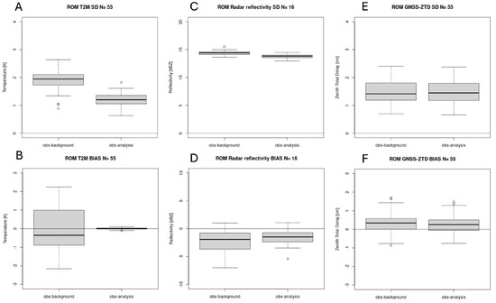
Figure 5.
Boxplots showing the standard deviation (SD) and bias of residuals for 2-meter temperature (2mT, A,B), radar reflectivity (C,D), and GNSS-derived Zenith Total Delay (ZTD, E,F) over multiple assimilation cycles in the Romanian demonstrator. Results compare the background forecast (obs-background) and the analysis (obs-analysis) residuals against observations.
For near-surface temperature, the results show a clear and substantial improvement after assimilation. Both the standard deviation and bias of 2mT (Figure 5A,B) residuals are significantly reduced in the analysis compared to the background forecast, confirming that assimilation effectively corrects temperature errors and stabilizes the forecast near the surface.
In the case of radar reflectivity (Figure 5C,D), the impact of assimilation is more moderate. The analysis shows a slight reduction in bias, indicating that the assimilation process helps to nudge the model towards better agreement with observed convective structures. However, the standard deviation remains largely unchanged. This behavior is expected, considering the high inherent variability and noise of radar observations, as well as the limited number of cases available, which constrain the potential for noticeable improvements in the spread of errors.
Regarding GNSS-ZTD (Figure 5E,F), assimilation leads to a slight reduction in bias, bringing the model’s representation of atmospheric water vapor closer to observations. However, the improvement remains within the observational error margin of approximately 1.5 cm, which is already accounted for in the 3D-Var assimilation scheme. Moreover, since the analyzed period did not include particularly intense meteorological events, the background forecast already provided an adequate representation of the vapor field, thus limiting the potential for further correction through assimilation.
In the Romanian demonstrator, vertical profiles collected by weather drones (Meteodrones) were assimilated whenever available, with the objective of assessing their contribution to improving the model’s representation of key atmospheric variables such as temperature, dew point temperature, wind speed, and wind direction. In total, eight assimilation cycles involving drone data were analyzed, corresponding to eight distinct time instances under different meteorological conditions. These profiles provided high-resolution information in the lower and middle troposphere, where traditional observations are typically sparse, making them particularly valuable for short-term forecast improvements. For an evaluation of the impact of cycling assimilation, see Appendix A.1.
Across all cases, the general trend confirms that the data assimilation (DA) step consistently improves the model state compared to both the background forecast (BF), which includes observations from previous cycles but not the most recent ones, and the open-loop (OL) simulation without any assimilation. The DA run systematically shows better agreement with observations, especially for thermodynamic variables, indicating the effective integration of drone data into the model.
However, the benefit of assimilation is not uniform across all cases and variables. In several instances, the BF does not significantly outperform the OL simulation, suggesting that the improvement introduced by previous assimilation cycles may dissipate depending on atmospheric dynamics and model characteristics. Additionally, while DA consistently improves temperature and humidity profiles, its impact on wind-related variables, particularly wind speed, exhibits greater variability, with performance depending on specific vertical levels and prevailing meteorological conditions.
Figure 6 provides a detailed example of this behavior, focusing on two consecutive assimilation cycles: 30 June 2024 at 21:00 UTC and 1 July 2024 at 00:00 UTC. The top panels show the detailed vertical profiles of temperature, dew point temperature, wind speed, and wind vector cosine similarity (WCOS), comparing the observations, analysis (DA), and background forecast (BF). In both cycles, the temperature and dew point profiles reveal that DA successfully corrects the biases present in BF, particularly near the surface and around 850–700 hPa.
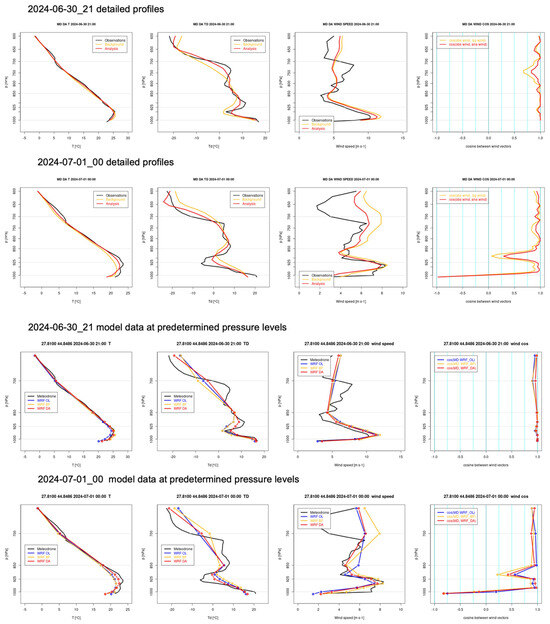
Figure 6.
Detailed vertical profiles (first two rows) of temperature (T, first column), dew point temperature (TD, second column), wind speed (third column), and the cosine of the angle between wind vectors (fourth column). The comparison is made between Meteodrones observations (black), background (orange), and DA analysis (red) to evaluate the impact of data assimilation on atmospheric variables at 21 UTC (first row) and 00 UTC (second row). Last two rows: Comparison of WRF model state in the OL (Open Loop, blue), BF (Background Forecast, orange), and DA (Data Assimilation, red) configurations against Meteodrone observations (black) at predefined pressure levels (dots refers to the model values available at the different pressure levels). The panels show the vertical profiles of temperature (T, first column), dew point temperature (TD, second column), wind speed (third column), and the cosine of the angle between wind vectors (fourth column) at 21 UTC (third row) and 00 UTC (fourth row).
Wind speed, which is generally underestimated by BF, is also better represented in the DA run, though some residual discrepancies persist in certain layers, especially near 850 hPa. The WCOS indicator shows that DA improves the directional agreement of wind vectors with observations, especially in the lower layers, though the improvement is less pronounced in the first cycle.
The lower panels of the figure present the same variables at predetermined pressure levels, adding the OL simulation (blue lines) for a comprehensive comparison. This enables the evaluation of the cumulative effect of assimilation cycles and assesses whether BF shows any improvement over the OL run. For temperature, all three simulations (OL, BF, DA) are relatively close to observations, with DA offering slight refinements, particularly near 925–850 hPa.
Dew point temperature shows a more pronounced improvement in DA, which reduces the dry bias present in OL and BF. Wind speed profiles confirm that OL underestimates wind intensity, BF provides partial correction, and DA yields the best alignment with observations, though discrepancies remain at mid-levels. WCOS similarly shows better agreement in DA, especially below 800 hPa, indicating an improvement in wind direction alignment after assimilation.
3.1.2. Extreme Event Forecasting: Convective Storms
At each site, multiple model runs were performed both with and without data assimilation to evaluate its potential added value in providing farmers with more accurate and precise forecasts. To achieve this, a sensitivity analysis was conducted by adjusting specific parameters within the MODE software to determine the optimal configuration for comparing predicted and observed weather patterns.
The French demonstrator assimilated data from various sources, including 2 m temperature, Zenith Total Delay (ZTD), and Meteodrone observations, to enhance the prediction of convective storms. The assimilation of these observations led to significant improvements in spatial and temporal accuracy, especially regarding the intensity and location of rainfall. By comparing simulations with and without data assimilation, it was found that assimilation improved the model’s ability to predict the evolution of convection, even in cases where storms were not particularly severe. The improved forecasts were particularly valuable for localized storm prediction, as they allowed for more accurate storm tracking and better-informed decision-making regarding disaster response and preparedness.
For the two French cases (18 June 2024 and 19 June 2024), the evaluation focused on the effect of assimilation on convective storm forecasts in the vicinity of the area of interest. These simulations were run in a nowcasting setup, with shorter forecasts initialized closer to the event. For both events, the verification timestep ranged from 12:00 to 24:00 UTC.
It is worth noting that in both cases, the rainfall events were neither particularly intense nor severe, and the recorded precipitation amounts were relatively low: these two days were selected because thunderstorms coincided with the availability of drone data for assimilation.
The analysis focused on lower precipitation thresholds, not exceeding 15 mm. This choice was made because setting a higher threshold would have limited the identification of sufficiently relevant objects in the verification process, thereby reducing the effectiveness of the evaluation.
In the first French case (18 June 2024), a threshold of 5 mm/12 h was adopted due to the low event intensity. Figure 7 (top) shows the objects recognized by MODE—both observed and forecasted. The left columns display WRF OL objects, while the right columns show WRF DA objects, for the 5 mm/12 h threshold. Blue contours represent observed objects; brown areas indicate forecasted objects; the red dot marks the Beaune site. Data assimilation notably improved the model’s performance, especially in terms of spatial pattern alignment, across all evaluated precipitation thresholds.
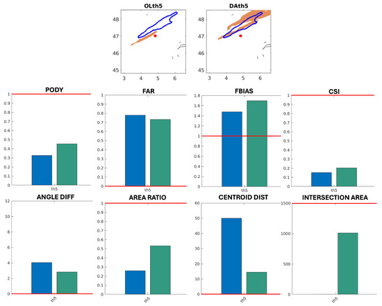
Figure 7.
Graphical representation of MODE output: on the top WRF OL (left column) and WRF DA (right column) for thresholds 5 mm/12 h where blue line contours represent observation objects, brown patterns represent forecasted objects, the red dot represents Beaune site; in the middle are plotted main statistical indices with the red lines the best scores for each index; on the bottom are plotted main parameters with the red lines the best scores for each index.
An examination of the statistical indices reveals that DA achieves a slightly higher Critical Success Index (CSI) than OL, indicating a better match between predicted and observed events. CSI excludes correct negatives and focuses solely on relevant forecasts, being sensitive to hits and penalizing both missed events and false alarms without distinguishing the source of error.
Both OL and DA exhibit a general overestimation of precipitation; however, DA slightly amplifies this tendency, as reflected by a higher FBIAS. This also impacts the POD index, with DA showing a higher value than OL—indicating that a greater fraction of observed events is correctly predicted. Additionally, DA presents a slightly lower FAR, indicating fewer false alarms.
Finally, the bottom panels of Figure 7 display the main MODE-derived attributes, comparing WRF OL (blue bars) and WRF DA (green bars). These confirm the superior spatial consistency of the DA run.
More specifically, the attribute “angle diff”, which measures the difference in orientation between forecasted and observed objects, is smaller in the DA run, indicating better alignment. Moreover, the “area ratio”, which quantifies overprediction or underprediction of spatial extent, the “intersection area”, which captures the overlap between forecast and observation, and the “centroid dist”, which measures spatial displacement, all confirm the superior performance of DA over OL.
Moving on to the second case study in France (20240619), it is evident that the afternoon thunderstorms were slightly more intense and widespread in the areas surrounding the site of interest.
Both model simulations, with and without data assimilation, successfully captured the spatial distribution and precipitation peaks. As a result, precipitation validation was conducted for two thresholds: 10 mm and 15 mm/12 h.
Figure 8 (top) displays the objects identified by MODE, both observed and predicted, offering a graphical representation of the MODE output. The left columns display the objects for WRF OL, while the right columns show WRF DA for the 10 mm and 15 mm/12 h thresholds. In the figure, blue contour lines represent observed objects, brown areas indicate forecasted objects, and the red dot marks the Beaune site.
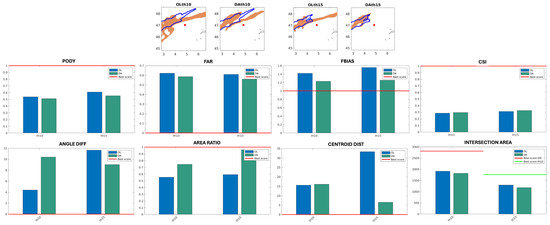
Figure 8.
Graphical representation by MODE output: (top) WRF OL and WRF DA for thresholds 10 mm and 15 mm/12h where blue line contours represent observation objects, brown patterns represent forecasted objects, the red dot represents Beaune site; (middle) are plotted main statistical indices with the red lines the best scores for each index; (bottom) are plotted main parameters with the red lines the best scores for each index.
A visual inspection reveals that both model runs accurately predicted the location of observed objects. However, DA demonstrates greater precision compared to OL, along with improved accuracy in terms of agreement between the forecast and actual observations.
Additionally, the figure presents statistical indices computed using MODE. These show that while both runs overestimate precipitation at both thresholds, data assimilation helps to slightly reduce this overestimation.
Since the PODY, FAR, and FBIAS indices should be interpreted together, it can be observed that in the OL run, where precipitation is more strongly overestimated, the probability of correctly predicting “yes” events is higher, resulting in a slightly greater PODY compared to DA. However, this also leads to a higher number of false alarms, as indicated by the greater FAR value for OL relative to DA.
Moreover, the CSI index, which measures the agreement between forecast and observed “yes” events, is very similar for both runs and thresholds, with a slight improvement in DA. Overall, DA improves spatial accuracy by refining feature localization and reducing overestimation compared to OL. While OL exhibits a higher Probability of Detection (PODY), it also has a higher False Alarm Ratio (FAR), meaning it tends to overpredict precipitation, leading to rainfall forecasts where none occurred. DA, although more conservative, reduces false alarms and produces a more realistic precipitation field, balancing detection capability with improved precision.
Finally, the bottom panels of Figure 8 show the main MODE-derived spatial attributes, comparing WRF OL (blue bars) and WRF DA (green bars). It is observed that the intersection area, representing the overlapping region between observed and forecasted objects, is very similar in both OL and DA, with a slight deterioration for DA.
However, looking at the area ratio, defined as the area of the predicted object divided by the area of the observed object and serving as an indicator of overestimation or underestimation, a clear improvement in DA is evident for both thresholds.
Again, considering the attribute “angle diff”, which indicates the angular difference between the axes of the forecasted and observed objects, DA performs better at the 15 mm threshold, while OL shows a smaller angle difference at 10 mm. This suggests that at 10 mm, the OL forecasted object is more aligned in orientation with the observed object, whereas at 15 mm, DA achieves better angular alignment.
Finally, regarding centroid distance—which quantifies the spatial displacement between the centroids of forecasted and observed objects, results are comparable between OL and DA at the 10 mm threshold, while DA shows a significantly smaller displacement at 15 mm. This indicates that at higher intensities, DA better captures the correct location of precipitation features.
3.2. Irrigation Advice Results from Agro-Hydrological Modeling
The irrigation advisory service of MAGDA provides farmers with forecasts of daily Irrigation Water Requirements (IWR) in m3/ha/day for short-term (2-day ahead) and medium-term (5-day ahead) forecast windows. Although sub-daily resolution may be of high interest under certain circumstances, this temporal resolution for outcomes was not explicitly requested by local farmers during the earlier phases of the research in which they were surveyed regarding their specific needs. According to the MAGDA irrigation approach adopted, IWR estimates represent the supplementary water that farmers may apply as irrigation to meet the crop’s daily water needs, based on weather forcings, crop development stage, and current soil moisture levels in the root zone.
Table 4 and Table 5 present irrigation recommendations—i.e., IWR values—issued at the SCDAB and Tetto-Bernardo pilot sites for the selected testing periods. The relative contribution of IWR to the crop reference evapotranspiration (IWR/ ratio) is also reported for comparison purposes.
Table 4.
Short-term forecasts of precipitation (), crop reference evapotranspiration (), and Irrigation Water Requirement (IWR) derived from different weather forecast products (DA and OL) at different testing dates and sites. IWR and in m3/ha/day. Total rainfall in the period measured at the site () and forecasted () are in mm.
Table 5.
Medium-term forecasts of precipitation (), crop reference evapotranspiration (), and Irrigation Water Requirement (IWR) derived from different weather forecast products (DA and OL) at different testing dates and sites. IWR and in m3/ha/day. Total rainfall in the period measured at the site () and forecasted () are in mm.
In SCDAB, with a higher sample size of forecasts than in Tetto-Bernardo, estimates of IWR and IWR/ ratios derived from weather forecasts with data assimilation (DA) were consistently higher than those retrieved for the benchmark case (OL) for both forecast windows. However, in Tetto-Bernardo, no clear difference was observed during the single testing period evaluated.
The results show that, in the SCDAB testing site, short-term (2-day ahead) forecasts of IWR and IWR/ were consistently higher than in medium-term (5-day ahead) forecasts (0.32–0.23 vs. 0.29–0.19, for DA-OL configurations, respectively) in the SCDAB testing site. No differences were detected in the Tetto-Bernardo site.
Recommendations for irrigation derived using the long-term DA forecast were in the same order of magnitude as irrigation quotas actually applied at the farm level following the traditional ICITID method (Table 6). Although not fully comparable due to the large conceptual differences between methods, in general, the ICITID method provided recommendations 35% lower than the MAGDA solution. These differences highlight the importance of accurately simulating the soil moisture dynamics and the climate forcings that control the water balance in the atmosphere-crop-soil continuum. The MAGDA solution may provide a clear advantage against current practices that rest on coarse approaches applied at county and regional scales.
Table 6.
Comparison of recommendations for irrigation derived from SPHY forced with long-term DA forecasts and the irrigation quotas already applied in the SCDAB pilot site in Romania. Precipitation values, Pobs and Pfcast, refer to the total rainfall in the testing period. ETc and IWR values are in m3/ha/day.
3.3. Farm Management System Integration: Communication to End Users
The versatility of the developed dashboard allowed the creation of distinct user accounts tailored to a wide range of user types—farmers or wine producers, cooperatives, advisors, and experts. Data access could be either unrestricted or limited to a specific demo site, depending on the user’s profile. Farmers who agreed to host part of MAGDA’s infrastructure were granted an account with access to all available data for their respective national demonstrator site (Figure 9).

Figure 9.
View of an Italian farmer’s dashboard with access to Meteodrone data and three in-crop in situ sensors.
Available data included Meteodrone flight data, in situ sensor data, forecast model outputs, and agro-hydrological results. Feedback from farmers was collected by Cap 2020 through interviews with users of its in situ sensors in France during the 2023 and 2024 campaigns, conducted independently of MAGDA, including users of the API that allows seamless data integration into third-party systems such as disease modeling applications or farm management software (Figure 10).
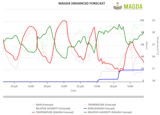
Figure 10.
Numerical weather forecast model using MAGDA’s infrastructure, with comparison to open-loop model forecasts, as displayed to farmers.
In the scope of MAGDA, stakeholders from all demonstrator sites were informed of new functionalities, and meetings were organized accordingly: France (Burgundy) in March 2023 and May 2024, Italy (Piedmont) in January 2025, and Romania (Brăila region) in March 2025. During these meetings, the functionalities of the dashboard and API were presented, and questions were answered.
Feedback led to adjustments in the dashboard, including a more efficient display of long time series and the possibility to define user-specific indicators, relatively simple calculations based on available data, adaptable to various crops and user profiles (Figure 11).
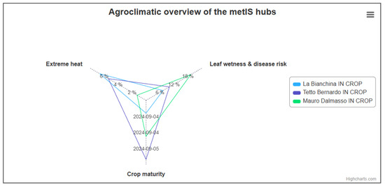
Figure 11.
Simple indicators based on MAGDA data can be customized and displayed by the farmer, e.g., disease risk, crop maturity, or water stress.
4. Discussion
A number of recent studies have investigated the integration of weather forecasts into irrigation scheduling models, highlighting both the benefits and limitations of such approaches. For example, [27] demonstrated that coupling real-time optimization with probabilistic forecasts, even when imperfect, can lead to significant gains in profitability and reductions in water. Likewise, [70] emphasized how forecast confidence, lead time, soil characteristics, and nitrogen availability interact to influence yield and environmental efficiency across different climatic zones. However, these studies are predominantly based on simulation frameworks that may face challenges when applied in operational settings, particularly under variable observational conditions or in areas with heterogeneous agricultural practices.
The MAGDA approach builds upon and extends these efforts by developing and validating an integrated, operational framework that combines high-resolution meteorological forecasting, data assimilation from multi-source sensor networks (GNSS, Meteodrones, in situ, and satellite data), and agro-hydrological modeling tailored to site-specific conditions. In doing so, MAGDA not only addresses the physical accuracy of short- and medium-term forecasts but also enhances their usability through an open-access dashboard and API, enabling direct integration with Farm Management Systems (FMS). This shift toward user-oriented design is crucial for the operational uptake of decision-support tools in agriculture.
Furthermore, while earlier studies such as [71] explored interactive systems where farmers could respond to model recommendations in real-time, MAGDA takes a complementary approach by embedding user feedback into the system design and validation process. This ensures that the forecasts and irrigation advisories are not only technically sound but also aligned with the real needs of diverse stakeholders. The integration of localized observational data and flexible assimilation cycles enables MAGDA to adapt dynamically to different agronomic contexts, offering both robustness and scalability.
Thus, MAGDA’s results offer a foundation for next-generation advisory systems that combine robust modeling with adaptive learning from farmer behavior. Expanding the observational network and further refining assimilation modules may enhance medium- and long-term forecast performance, potentially overcoming some of the limitations of short-term forecasting observed in prior work [27].
From the GNSS sensors’ point of view, PPP-based integrated water-vapor (IWV) retrievals within MAGDA, using both geodetic-grade and low-cost GNSS receivers, confirm the robustness of this technique, in accordance with the work by [72,73,74]. In contrast, deriving soil moisture from GNSS reflectometry proved more challenging: in the MAGDA project, sensors relied solely on low-cost units, and agricultural deployment introduced uneven terrain, seasonal snow cover, and dense, rapidly changing vegetation that limited the usage of SNR-based reflections. Although controlled-environment studies have recently reported encouraging accuracy [75,76,77], MAGDA’s field experience underscores the practical limitations that still constrain large-scale operational use.
- Data assimilation impact: The DA framework showed consistent improvements in model performance, especially for 2-meter temperature (2mT) forecasts. Radar reflectivity and Zenith Total Delay (ZTD) assimilation also improved forecasts, though their benefit was more constrained by observational noise.
- Vertical profiling via drones: The assimilation of eight Meteodrone-based vertical profiles significantly refined thermodynamic fields in the planetary boundary layer and lower troposphere. While improvements in temperature and humidity were consistent, results for wind speed were more variable, underscoring the need for more robust wind-related observational data.
- Convective storm prediction: DA improved key forecast skill metrics for convective storms, such as Probability of Detection (PODY) and False Alarm Ratio (FAR), highlighting better storm localization and reduced false positives.
- Demonstrator-specific outcomes: In the French demonstrator (nowcasting of convective storms), DA notably enhanced spatial accuracy and reduced false alarms. In contrast, in the Romanian and Italian demonstrators focused on irrigation, DA improved model initialization but had a subtler effect on precipitation forecasts due to already moderate rainfall events and longer forecasts losing the assimilation effect that typically influences the first 6–12 h.
- Irrigation strategy refinement: Even when rainfall forecasts were similar between DA and OL runs, DA contributed to more consistent and realistic system states. This led to better-informed irrigation strategies, with potential water savings compared to traditional approaches based only on reference evapotranspiration. A comparison with the ICITID method used operationally at the Romanian pilot site showed that MAGDA’s long-term DA forecasts produced irrigation recommendations of the same order of magnitude. However, the ICITID method provided quotas approximately 35% lower than MAGDA. This discrepancy highlights the value of simulating soil moisture dynamics and climate forcings in a coupled atmosphere–crop–soil framework, offering a potential advantage over coarse, county-scale approaches.
- Sensor-driven initialization: The hydrological models benefited from initialization with in situ soil moisture sensors. Although not formally compared to satellite-based initializations, these site-specific measurements appear more suitable for field-scale applications.
- Update frequency: More frequent forecast updates (every 2 days vs. 5) led to better irrigation efficiency, reinforcing the value of short-term updates in operational advisory systems.
- User engagement and customization: The MAGDA dashboard demonstrated a high degree of operational flexibility and user-centered design. Throughout the project, multiple stakeholder engagement activities—including field demonstrations, user interviews, and national workshops—allowed for iterative refinement of the system. Feedback from farmers, cooperatives, and technical advisors led to improvements such as the display of long time series, the creation of customized indicators (e.g., crop-specific water stress or disease risk), and the simplification of data visualization to enhance usability across different user profiles.
- Alignment with EU policy and strategic integration: MAGDA’s outcomes directly contribute to the broader objectives of the European Green Deal and the Common Agricultural Policy (CAP) by promoting sustainable water management, resilience to climate variability, and resource efficiency. The system’s architecture, featuring an open API and modular services, facilitates interoperability with existing Farm Management Systems (FMS), enabling adoption by both public-sector platforms and commercial agri-tech providers. Furthermore, the project’s clustering efforts and alignment with other EU-funded initiatives have strengthened the strategic visibility and replicability of MAGDA across European agricultural value chains.
- Economic sustainability and exploitation potential: The MAGDA system, as implemented and tested, proved to be an economically sustainable solution for high-value crop contexts, thanks to the scalability of its sensor infrastructure and the modularity of its digital services. The project established the groundwork for both commercial and non-commercial uptake pathways, including precision agriculture solution providers, public authorities responsible for water and risk management, and environmental research institutions. This multi-channel exploitation strategy, coupled with the system’s demonstrated adaptability, increases the potential for long-term operational deployment
5. Conclusions
Climate change and the growing pressure on water resources underscore the urgent need for forecasting systems that are more localized, accurate, and actionable to support decision-making in agriculture. In response to this challenge, the MAGDA project was designed to develop and assess an integrated framework that combines high-resolution numerical weather prediction, advanced data assimilation techniques, field-deployed observational infrastructure (including drone-based atmospheric profiling and in situ soil moisture monitoring), agro-hydrological modeling, and a user-centric digital platform. The overarching goal was not only to enhance the physical accuracy of meteorological forecasts, but also to ensure their direct applicability in operational contexts, such as irrigation scheduling and convective weather risk management, across both farm and regional scales.
The integrated MAGDA system was tested at three pilot sites representing diverse climatic and agricultural conditions across Europe. The results demonstrate that data assimilation notably improves the representation of the atmospheric state, particularly for near-surface thermodynamic variables, leading to more accurate and stable forecasts. The French demonstrator clearly illustrated the added value of assimilation for convective storm prediction, improving both spatial precision and detection capability. In the irrigation-focused demonstrators in Romania and Italy, the assimilation of drone-based and ground-based observations led to improved soil moisture initialization and forecast realism, even under moderate rainfall scenarios where open-loop forecasts were already reasonably accurate. Significantly, the integration of meteorological forecasts with a soil moisture-sensitive crop irrigation model enabled more adaptive and efficient water use strategies than those based on conventional crop reference evapotranspiration alone.
Local, high-resolution observational data proved particularly effective in increasing the field-scale relevance of forecasts, where satellite-derived products often fall short in spatial and temporal specificity. Furthermore, the analysis highlighted the operational advantage of frequent forecast updates (e.g., every two days), which resulted in reduced irrigation requirements without compromising forecast accuracy.
Key contributions of the MAGDA project can be summarized as follows:
- Multi-source assimilation: Integration of GNSS, drone-based profiling, radar, and in situ sensors into a high-resolution forecasting chain.
- Improved forecast accuracy: Enhanced short-term and very-short-term forecasts for both convective events and agricultural variables, particularly near-surface temperature and moisture.
- Agro-hydrological coupling: Operational linkage of weather forecasts with soil-moisture sensitive irrigation modeling (SPHY), enabling site-specific irrigation recommendations.
- Operational dashboards: Development of a user-oriented interface and open APIs for integration with Farm Management Systems.
- Validated impact: Demonstrated improvements in forecast skill, irrigation efficiency, and usability across three European pilot sites with diverse climatic and agricultural conditions.
These findings support the conclusion that co-designed, integrated forecasting systems, combining assimilation, observation, modeling, and stakeholder-oriented interfaces, can effectively bridge the gap between scientific forecasting capabilities and real-world agricultural needs. While further refinement is still needed in background error characterization and observation network optimization, the framework developed through MAGDA lays a solid foundation for operational, climate-resilient agro-meteorological services, offering a cost-effective solution suitable for real-world deployment in diverse agricultural contexts.
Author Contributions
Conceptualization, M.L. and E.R.; methodology, M.L., S.C. and E.R.; software, A.G., A.F., L.H., F.U., Z.C. and J.O.; validation, E.O., A.F.-R. and S.B.; formal analysis, F.R. and I.O.; investigation, M.M.; resources, M.L., D.H. and M.d.K.; data curation, E.R., J.O. and Z.C.; writing—original draft preparation, M.L., S.C., J.O. and A.V.; writing—review and editing, E.R., F.R. and A.V.; visualization, J.O.; supervision, E.R.; project administration, A.G.; funding acquisition, E.R. and M.M. All authors have read and agreed to the published version of the manuscript.
Funding
This research was funded by Horizon Europe/EUSPA through the MAGDA (Meteorological Assimilation from Galileo and Drones for Agriculture) project grant number 101082189.
Data Availability Statement
The datasets presented in this article are not readily available because they include measurements of parameters related to private end-users’ agricultural fields, thus potentially confidential/sensitive. Requests to access the datasets should be directed to the corresponding author.
Acknowledgments
The data and results obtained within the MAGDA project are available upon request for non-commercial purposes.
Conflicts of Interest
Authors Stefano Barindelli, Alessandro Fumagalli, Andrea Gatti, Eugenio Realini were employed by the company Geomatics Research & Development srl. Authors Sergio Contreras, Amelia Fernández-Rodríguez, Martijn de Klerk were employed by the company FutureWater. Authors Lukas Hammerschmidt, Fabiola Ramelliwere employed by the company Meteomatics AG. Authors Damir Haskovic, Aso Validi were employed by the company MINDS & SPARKS GmbH. Author Julien Orensanz was employed by the company CAP2020. The remaining authors declare that the research was conducted in the absence of any commercial or financial relationships that could be construed as a potential conflict of interest.
Abbreviations
The following abbreviations are used in this manuscript:
| 2mT | 2 m Temperature |
| BF | Background Forecast |
| DA | Data Assimilation |
| EPN | European Permanent Network |
| FMS | Farm Management System |
| GNSS | Global Navigation Satellite System |
| NWP | Numerical Weather Prediction |
| OL | Open Loop |
| PPP | Precise Point Positioning |
| ZTD | Zenith Total Delay |
Appendix A
Appendix A.1
Table A1.
Features available in the Farm Management System Dashboard.
Table A1.
Features available in the Farm Management System Dashboard.
| Type of Feature | Description |
|---|---|
| User management | Possibility to easily give access to a subset of data to a given set of users. (i.e., farmers can have access to data on the location of their farm, local advisors on a demo site, MAGDA stakeholders and partners on all demo’s sites data) |
| Summary display | Quick view of all in situ sensors status together with GNSS stations status and Meteodrone status. Last data & alerts for in situ, Meteodrone, hydrological & numerical weather model in a block view. |
| In situ data display | possibility to display in situ sensors data over various time windows. |
| Meteodrone data display | Possibility to display last Meteodrone flight data (vertical profile) |
| Hydrological model results display | Possibility to display useful irrigation advice information on a map based view on the different points of interest of a demo site. |
| Weather numerical model display | Possibility to display different versions of a past forecast (i.e. with full assimilation of sensors or not), together with actual measurements. |
| User indicators | Possibility to define indicators of interest using data from MAGDA’s sensors and models. Indicators is a way to display synthetic decision making data calculated using raw data. They usually are more simple than a model. |
| Data visualization fine tuning | Possibility for the user to select the way data can be displayed, for example when selecting a period of X days between two dates, should the data be displayed as hourly data or daily data. |
| Data download | Possibility for the user to download short or extended periods of data that he wishes to use, in a readable, convenient format. |
| translation | The dashboard should be easy to translate in any language using translation files. |
| Responsive interface | The dashboard should be navigable and easily usable on personal computers, tablets, phones. |
Appendix A.2
In this Appendix, an initial evaluation of the assimilation performance across the assimilation cycles is presented, offering insights into how forecast errors propagate throughout the assimilation process. Since the indices are calculated by comparing observations to the background at each assimilation step, they allow for tracking the evolution of errors as the forecast progresses. The behavior is similar with all variables, thus, only the 2mT will be discussed here for the sake of brevity. The Romanian demonstrator is used because more cases are available on that site, allowing for a wider boxplot statistics, but similar behavior is shown also for the Italian site. The assimilation of 2mT data revealed fluctuations in forecast bias across the assimilation cycles (Figure A1A,B). Initially, a positive bias (−1 °C to −2 °C) in the second cycle, and then returned to positive values (1 °C) by the third cycle. These fluctuations indicate that the assimilation process introduces short-term corrections, which might be refined further to improve consistency. Despite these oscillations in bias, the standard deviation (SD) of temperature remained relatively stable at around 2 °C throughout the assimilation cycles, with only a slight decrease observed at the final cycle, indicating some stabilization. Looking to a specific case taken as an example, it is possible to provide further information on assimilation behavior. Figure A1C illustrates the evolution of 2mT residuals (observations minus background and analysis) over the first 6 h from the initial analysis time, highlighting the effect of the three assimilation cycles. The thick dark line represents the mean residuals, while the thin blue lines indicate the standard deviation. A noticeable reduction in residuals and spread is observed after each assimilation cycle, demonstrating an improvement in forecast accuracy and a decrease in uncertainty. In particular, the distinct discontinuity around hour 3 reflects the direct impact of the second assimilation cycle, which further corrects the forecast and reduces the bias. Moreover, a reduced increase in forecast error is evident between the second and third assimilation cycles compared to the period between the first and second cycles. This behavior indicates not only the corrective effect of cyclic data assimilation on the model state but also its positive role in limiting error propagation in subsequent forecast hours.
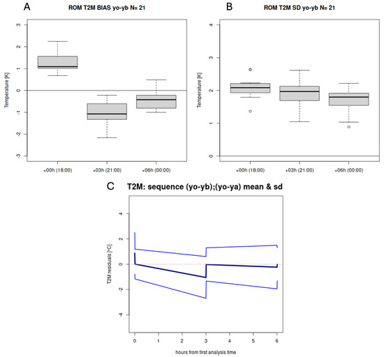
Figure A1.
(A,B): Boxplots of BIAS (A) and Standard Deviation (B) of 2mT assimilation. The boxplots represent the observation-background at each assimilation cycle (18-21-00 UTC). (C): example of mean residuals of observations with respect to the background (yo-yb) and analysis (yo-ya) with associated dispersion.
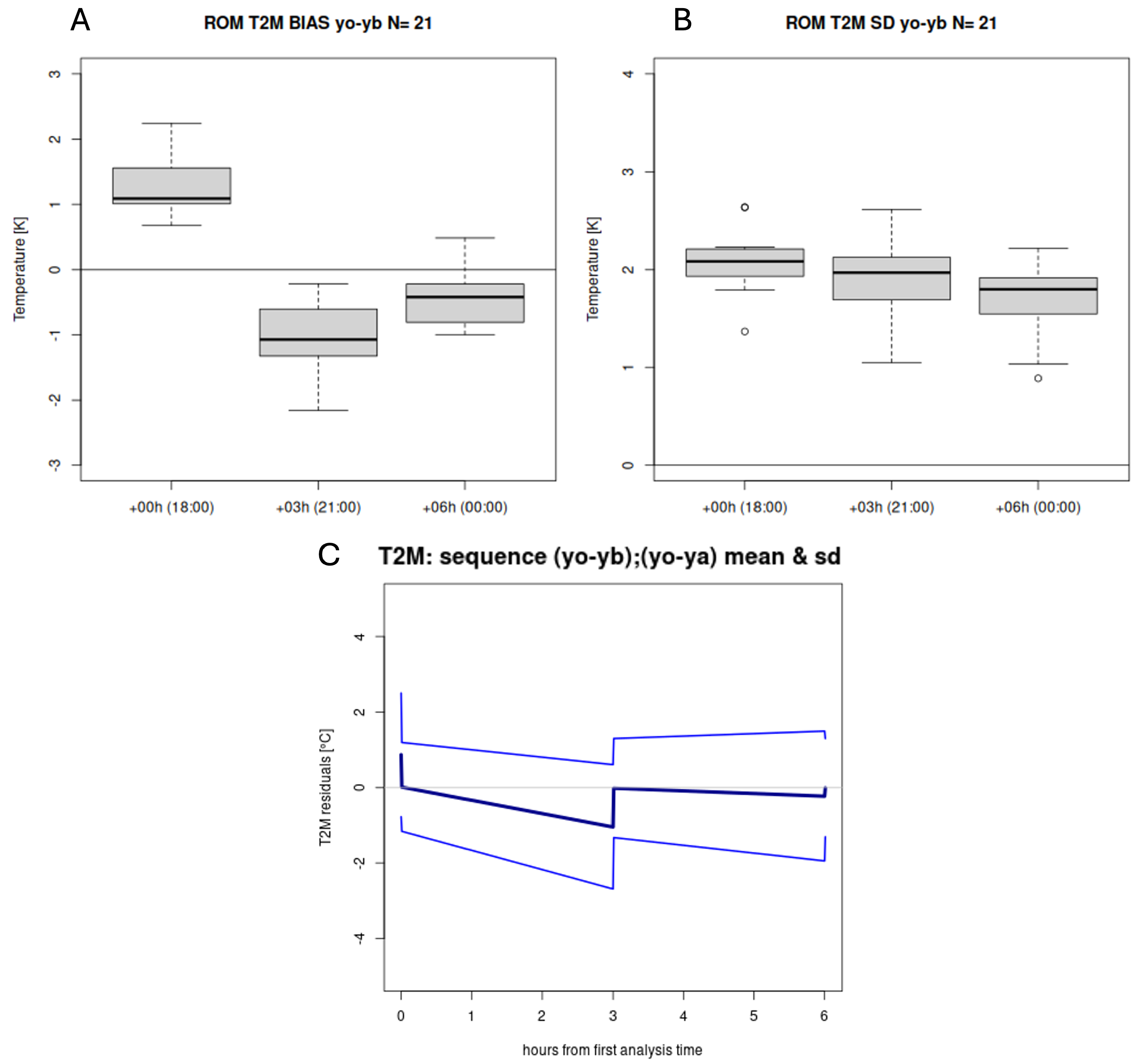
To assess the effectiveness of the cyclic data assimilation approach for the Meteodrones observations, Figure A2 shows the vertical profiles of temperature (T), relative humidity (RH), and wind vector orientation (expressed as cosine similarity) to evaluate the impact of sequential data assimilation using a 3DVar scheme. The comparison is made between the open loop (OL) simulation, which does not assimilate any observations (blue line), and the assimilation runs, which include the assimilation of Meteodrone profiles (black line) with different observation error settings. The left panels display the forecast at 00 UTC after assimilating the first observation profile collected at 21 UTC (red and pink lines), while the right panels show the analysis at 00 UTC after assimilating the second profile collected at 00 UTC. The results highlight how the information from the first assimilation cycle is effectively retained in the model forecast, improving alignment with observations compared to the OL simulation. The subsequent assimilation at 00 UTC further refines the model state, demonstrating a cumulative improvement, particularly visible in relative humidity and wind orientation profiles. The sensitivity test, represented by the red (small error) and pink (large error) lines, indicates that even when assigning a smaller observation error, the assimilation system successfully integrates the observational data without degrading the solution, confirming the robustness of the setup. Overall, the figure demonstrates how cyclic variational assimilation contributes not only to correcting the model state at analysis time but also to reducing forecast errors and preserving improvements across successive assimilation cycles. This evaluation was carried out on a set of cases during the demonstrator phase to verify that such impacts are consistently observed across different situations. Naturally, the degree to which the assimilation effect is retained from one cycle to the next may vary slightly depending on the type of event and the prevailing atmospheric dynamics.
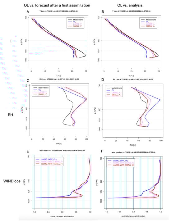
Figure A2.
(A,B): Example of vertical profiles comparing the Open Loop (OL) simulation with forecasts after a first data assimilation (left column: A,C,E) and with the analysis (right column: B,D,F). (A,B) Temperature profiles (T, in °C) as a function of pressure (p, in hPa). (C,D) Relative Humidity profiles (RH, in %) versus pressure. (E,F) wind vector orientation expressed as cosine similarity. Lines represent the Metedrone observations (black), the OL (blue), and different assimilation experiments (red and pink lines show two different simulations performed with different observational errors).
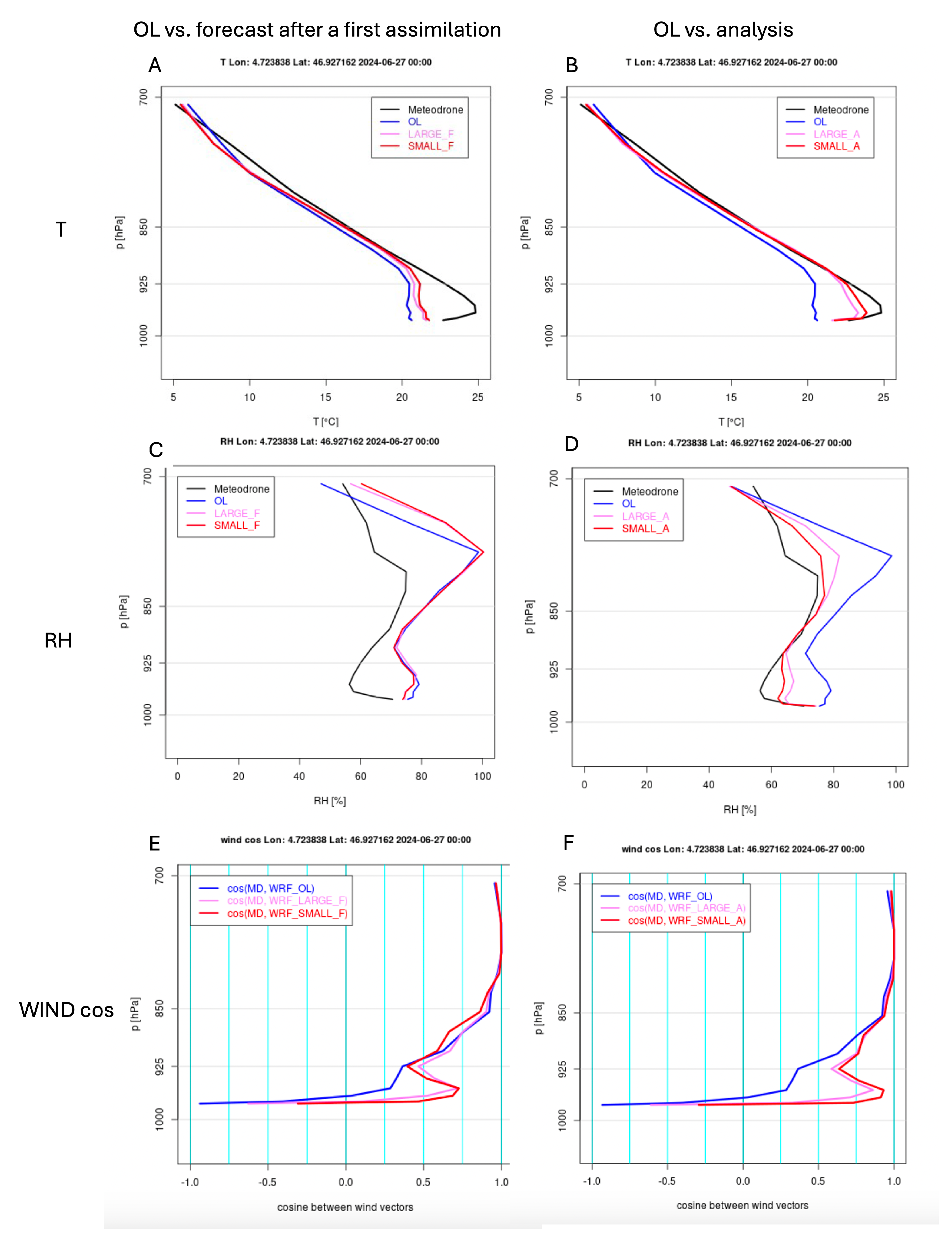
References
- Blanchard-Wrigglesworth, E.; Bilbao, R.; Donohoe, A.; Materia, S. Record warmth of 2023 and 2024 resulted from ENSO transition and Northern Hemisphere absorbed shortwave anomalies. Authorea Prepr. 2025. [Google Scholar] [CrossRef]
- Koech, R.; Langat, P. Improving irrigation water use efficiency: A review of advances, challenges and opportunities in the Australian context. Water 2018, 10, 1771. [Google Scholar] [CrossRef]
- Kleynen, O.; Leemans, V.; Destain, M.F. Development of a multi-spectral vision system for the detection of defects on apples. J. Food Eng. 2005, 69, 41–49. [Google Scholar] [CrossRef]
- Riquelme, M.; Barreiro, P.; Ruiz-Altisent, M.; Valero, C. Olive classification according to external damage using image analysis. J. Food Eng. 2008, 87, 371–379. [Google Scholar] [CrossRef]
- Simon, G. Review on rain induced fruit cracking of sweet cherries (Prunus avium L.), its causes and the possibilities of prevention. Int. J. Hortic. Sci. 2006, 12, 27–35. [Google Scholar] [CrossRef]
- Cutforth, H.W.; McGinn, S.M.; McPhee, K.E.; Miller, P.R. Adaptation of pulse crops to the changing climate of the Northern Great Plains. Agron. J. 2007, 99, 1684–1699. [Google Scholar] [CrossRef]
- Barnett, T.P.; Adam, J.C.; Lettenmaier, D.P. Potential impacts of a warming climate on water availability in snow-dominated regions. Nature 2005, 438, 303–309. [Google Scholar] [CrossRef]
- Bales, R.C.; Molotch, N.P.; Painter, T.H.; Dettinger, M.D.; Rice, R.; Dozier, J. Mountain hydrology of the western United States. Water Resour. Res. 2006, 42. [Google Scholar] [CrossRef]
- Viviroli, D.; Dürr, H.H.; Messerli, B.; Meybeck, M.; Weingartner, R. Mountains of the world, water towers for humanity: Typology, mapping, and global significance. Water Resour. Res. 2007, 43. [Google Scholar] [CrossRef]
- Faurès, J.M.; Hoogeveen, J.; Bruinsma, J. The FAO Irrigated Area Forecast for 2030; FAO: Rome, Italy, 2002; pp. 1–14. [Google Scholar]
- Fouial, A.; Lamaddalena, N.; Rodriguez Diaz, J.A. Generating hydrants’ configurations for efficient analysis and management of pressurized irrigation distribution systems. Water 2020, 12, 204. [Google Scholar] [CrossRef]
- Hristov, J.; Toreti, A.; Pérez Domínguez, I.; Dentener, F.; Fellmann, T.; Elleby, C.; Ceglar, A.; Fumagalli, D.; Niemeyer, S.; Cerrani, I.; et al. Analysis of Climate Change Impacts on EU Agriculture by 2050; Publications Office of the European Union: Luxembourg, 2020. [Google Scholar]
- Southworth, J.; Randolph, J.; Habeck, M.; Doering, O.; Pfeifer, R.; Rao, D.G.; Johnston, J. Consequences of future climate change and changing climate variability on maize yields in the midwestern United States. Agric. Ecosyst. Environ. 2000, 82, 139–158. [Google Scholar] [CrossRef]
- Hatfield, J.L.; Boote, K.J.; Kimball, B.A.; Ziska, L.; Izaurralde, R.C.; Ort, D.; Thomson, A.M.; Wolfe, D. Climate impacts on agriculture: Implications for crop production. Agron. J. 2011, 103, 351–370. [Google Scholar] [CrossRef]
- Cancela, J.J.; González, X.P.; Vilanova, M.; Mirás-Avalos, J.M. Water management using drones and satellites in agriculture. Water 2019, 11, 874. [Google Scholar] [CrossRef]
- Navarro-Hellín, H.; Martinez-del Rincon, J.; Domingo-Miguel, R.; Soto-Valles, F.; Torres-Sánchez, R. A decision support system for managing irrigation in agriculture. Comput. Electron. Agric. 2016, 124, 121–131. [Google Scholar] [CrossRef]
- Rinaldi, M.; He, Z. Decision support systems to manage irrigation in agriculture. Adv. Agron. 2014, 123, 229–279. [Google Scholar]
- Giannakis, E.; Bruggeman, A.; Djuma, H.; Kozyra, J.; Hammer, J. Water pricing and irrigation across Europe: Opportunities and constraints for adopting irrigation scheduling decision support systems. Water Sci. Technol. Water Supply 2016, 16, 245–252. [Google Scholar] [CrossRef]
- Bonfante, A.; Monaco, E.; Manna, P.; De Mascellis, R.; Basile, A.; Buonanno, M.; Cantilena, G.; Esposito, A.; Tedeschi, A.; De Michele, C.; et al. LCIS DSS—An irrigation supporting system for water use efficiency improvement in precision agriculture: A maize case study. Agric. Syst. 2019, 176, 102646. [Google Scholar] [CrossRef]
- D’Urso, G.; Richter, K.; Calera, A.; Osann, M.; Escadafal, R.; Garatuza-Pajan, J.; Hanich, L.; Perdigão, A.; Tapia, J.; Vuolo, F. Earth Observation products for operational irrigation management in the context of the PLEIADeS project. Agric. Water Manag. 2010, 98, 271–282. [Google Scholar] [CrossRef]
- Campos, I.; Neale, C.M.; Calera, A.; Balbontín, C.; González-Piqueras, J. Assessing satellite-based basal crop coefficients for irrigated grapes (Vitis vinifera L.). Agric. Water Manag. 2010, 98, 45–54. [Google Scholar] [CrossRef]
- Galleguillos, M.; Jacob, F.; Prévot, L.; French, A.; Lagacherie, P. Comparison of two temperature differencing methods to estimate daily evapotranspiration over a Mediterranean vineyard watershed from ASTER data. Remote Sens. Environ. 2011, 115, 1326–1340. [Google Scholar] [CrossRef]
- Vanino, S.; Pulighe, G.; Nino, P.; De Michele, C.; Falanga Bolognesi, S.; D’Urso, G. Estimation of evapotranspiration and crop coefficients of tendone vineyards using multi-sensor remote sensing data in a Mediterranean environment. Remote Sens. 2015, 7, 14708–14730. [Google Scholar] [CrossRef]
- Vuolo, F.; Essl, L.; Atzberger, C. Costs and benefits of satellite-based tools for irrigation management. Front. Environ. Sci. 2015, 3, 52. [Google Scholar] [CrossRef]
- Gowing, J.; Ejieji, C. Real-time scheduling of supplemental irrigation for potatoes using a decision model and short-term weather forecasts. Agric. Water Manag. 2001, 47, 137–153. [Google Scholar] [CrossRef]
- Wang, D.; Cai, X. Irrigation scheduling—Role of weather forecasting and farmers’ behavior. J. Water Resour. Plan. Manag. 2009, 135, 364–372. [Google Scholar] [CrossRef]
- Cai, X.; Hejazi, M.I.; Wang, D. Value of probabilistic weather forecasts: Assessment by real-time optimization of irrigation scheduling. J. Water Resour. Plan. Manag. 2011, 137, 391–403. [Google Scholar] [CrossRef]
- Perera, K.C.; Western, A.W.; Robertson, D.E.; George, B.; Nawarathna, B. Ensemble forecasting of short-term system scale irrigation demands using real-time flow data and numerical weather predictions. Water Resour. Res. 2016, 52, 4801–4822. [Google Scholar] [CrossRef]
- Linker, R.; Sylaios, G. Efficient model-based sub-optimal irrigation scheduling using imperfect weather forecasts. Comput. Electron. Agric. 2016, 130, 118–127. [Google Scholar] [CrossRef]
- Cao, J.; Tan, J.; Cui, Y.; Luo, Y. Irrigation scheduling of paddy rice using short-term weather forecast data. Agric. Water Manag. 2019, 213, 714–723. [Google Scholar] [CrossRef]
- Simionesei, L.; Ramos, T.B.; Brito, D.; Jauch, E.; Leitão, P.C.; Almeida, C.; Neves, R. Numerical simulation of soil water dynamics under stationary sprinkler irrigation with Mohid-Land. Irrig. Drain. 2016, 65, 98–111. [Google Scholar] [CrossRef]
- Hassan-Esfahani, L.; Torres-Rua, A.; McKee, M. Assessment of optimal irrigation water allocation for pressurized irrigation system using water balance approach, learning machines, and remotely sensed data. Agric. Water Manag. 2015, 153, 42–50. [Google Scholar] [CrossRef]
- Ukhurebor, K.E.; Adetunji, C.O.; Olugbemi, O.T.; Nwankwo, W.; Olayinka, A.S.; Umezuruike, C.; Hefft, D.I. Precision agriculture: Weather forecasting for future farming. In AI, Edge and IoT-Based Smart Agriculture; Elsevier: Amsterdam, The Netherlands, 2022; pp. 101–121. [Google Scholar]
- Chitu, Z.; Tomei, F.; Villani, G.; Di Felice, A.; Zampelli, G.; Paltineanu, I.C.; Visinescu, I.; Dumitrescu, A.; Bularda, M.; Neagu, D.; et al. Improving Irrigation Scheduling Using MOSES Short-Term Irrigation Forecasts and In Situ Water Resources Measurements on Alluvial Soils of Lower Danube Floodplain, Romania. Water 2020, 12, 520. [Google Scholar] [CrossRef]
- Powell, J.; Reinhard, S. Measuring the effects of extreme weather events on yields. Weather Clim. Extrem. 2016, 12, 69–79. [Google Scholar] [CrossRef]
- Doblas-Reyes, F.; Garcia, A.; Hansen, J.; Mariani, L.; Nain, A.; Ramesh, K.; Venkataraman, R. Weather and climate forecasts for agriculture. Guide Agric. Meteorol. Pract. 2003, 57. Available online: https://citeseerx.ist.psu.edu/document?repid=rep1&type=pdf&doi=adf3379a84f0e48b0a835c783be924078ae421a1 (accessed on 22 May 2025).
- Cogato, A.; Meggio, F.; De Antoni Migliorati, M.; Marinello, F. Extreme weather events in agriculture: A systematic review. Sustainability 2019, 11, 2547. [Google Scholar] [CrossRef]
- Bevis, M.; Businger, S.; Herring, T.A.; Rocken, C.; Anthes, R.A.; Ware, R.H. GPS meteorology: Remote sensing of atmospheric water vapor using the global positioning system. J. Geophys. Res. Atmos. 1992, 97, 15787–15801. [Google Scholar] [CrossRef]
- Lagasio, M.; Parodi, A.; Pulvirenti, L.; Meroni, A.N.; Boni, G.; Pierdicca, N.; Marzano, F.S.; Luini, L.; Venuti, G.; Realini, E.; et al. A synergistic use of a high-resolution numerical weather prediction model and high-resolution Earth observation products to improve precipitation forecast. Remote Sens. 2019, 11, 2387. [Google Scholar] [CrossRef]
- Chew, C.; Small, E.E.; Larson, K.M. An algorithm for soil moisture estimation using GPS-interferometric reflectometry for bare and vegetated soil. GPS Solut. 2016, 20, 525–537. [Google Scholar] [CrossRef]
- Guzinski, R.; Nieto, H.; Sandholt, I.; Karamitilios, G. Modelling high-resolution actual evapotranspiration through Sentinel-2 and Sentinel-3 data fusion. Remote Sens. 2020, 12, 1433. [Google Scholar] [CrossRef]
- Skamarock, W.C.; Klemp, J.B.; Dudhia, J.; Gill, D.O.; Barker, D.M.; Duda, M.; Wang, X.Y.; Wang, W.; Power, J.G. A Description of the Advanced Research WRF Version 3; NCAR Technical Note NCAR/TN-475+STR; National Center for Atmospheric Research: Boulder, CO, USA, 2008; p. 113. [Google Scholar] [CrossRef]
- Fiori, E.; Ferraris, L.; Molini, L.; Siccardi, F.; Kranzlmueller, D.; Parodi, A. Triggering and evolution of a deep convective system in the Mediterranean sea: Modelling and observations at a very fine scale. Q. J. R. Meteorol. Soc. 2017, 143, 927–941. [Google Scholar] [CrossRef]
- Lagasio, M.; Parodi, A.; Procopio, R.; Rachidi, F.; Fiori, E. Lightning potential index performances in multimicrophysical cloud-resolving simulations of a back-building mesoscale convective system: The Genoa 2014 event. J. Geophys. Res. Atmos. 2017, 122, 4238–4257. [Google Scholar] [CrossRef]
- Lagasio, M.; Silvestro, F.; Campo, L.; Parodi, A. Predictive capability of a high-resolution hydrometeorological forecasting framework coupling WRF cycling 3dvar and Continuum. J. Hydrometeorol. 2019, 20, 1307–1337. [Google Scholar] [CrossRef]
- Lagasio, M.; Fagugli, G.; Ferraris, L.; Fiori, E.; Gabellani, S.; Masi, R.; Mazzarella, V.; Milelli, M.; Parodi, A.; Pignone, F.; et al. A Complete meteo/hydro/hydraulic chain application to support early warning and monitoring systems: The Apollo Medicane use case. Remote Sens. 2022, 14, 6348. [Google Scholar] [CrossRef]
- Hong, S.Y.; Lim, J.O.J. The WRF single-moment 6-class microphysics scheme (WSM6). Asia-Pac. J. Atmos. Sci. 2006, 42, 129–151. [Google Scholar]
- Hong, S.Y.; Noh, Y.; Dudhia, J. A new vertical diffusion package with an explicit treatment of entrainment processes. Mon. Weather Rev. 2006, 134, 2318–2341. [Google Scholar] [CrossRef]
- Iacono, M.J.; Delamere, J.S.; Mlawer, E.J.; Shephard, M.W.; Clough, S.A.; Collins, W.D. Radiative forcing by long-lived greenhouse gases: Calculations with the AER radiative transfer models. J. Geophys. Res. Atmos. 2008, 113. [Google Scholar] [CrossRef]
- Smirnova, T.G.; Brown, J.M.; Benjamin, S.G.; Kim, D. Parameterization of cold season processes in the MAPS land-surface scheme. J. Geophys. Res. 2000, 105, 4077–4086. [Google Scholar] [CrossRef]
- Barker, D.; Huang, X.Y.; Liu, Z.; Auligné, T.; Zhang, X.; Rugg, S.; Ajjaji, R.; Bourgeois, A.; Bray, J.; Chen, Y.; et al. The weather research and forecasting model’s community variational/ensemble data assimilation system: WRFDA. Bull. Am. Meteorol. Soc. 2012, 93, 831–843. [Google Scholar] [CrossRef]
- Anderson, E.; Järvinen, H. Variational quality control. Q. J. R. Meteorol. Soc. 1999, 125, 697–722. [Google Scholar] [CrossRef]
- Lagasio, M.; Campo, L.; Milelli, M.; Mazzarella, V.; Poletti, M.L.; Silvestro, F.; Ferraris, L.; Federico, S.; Puca, S.; Parodi, A. SWING, the Score-Weighted Improved NowcastinG algorithm: Description and application. Water 2022, 14, 2131. [Google Scholar] [CrossRef]
- Poletti, M.L.; Lagasio, M.; Parodi, A.; Milelli, M.; Mazzarella, V.; Federico, S.; Campo, L.; Falzacappa, M.; Silvestro, F. Hydrological verification of two rainfall short-term forecasting methods with floods anticipation perspective. J. Hydrometeorol. 2024, 25, 541–561. [Google Scholar] [CrossRef]
- Parrish, D.F.; Derber, J.C. The National Meteorological Center’s spectral statistical-interpolation analysis system. Mon. Weather Rev. 1992, 120, 1747–1763. [Google Scholar] [CrossRef]
- Goga, K.; Pilosu, L.; Parodi, A.; Lagasio, M.; Terzo, O. Performance of wrf cloud resolving simulations with data assimilation on public cloud and hpc environments. In Proceedings of the Complex, Intelligent, and Software Intensive Systems: Proceedings of the 12th International Conference on Complex, Intelligent, and Software Intensive Systems (CISIS-2018), Matsue, Japan, 4–6 July 2018; Springer: Cham, Switzerland, 2019; pp. 161–171. [Google Scholar]
- Burlando, M.; Romanic, D.; Boni, G.; Lagasio, M.; Parodi, A. Investigation of the weather conditions during the collapse of the Morandi Bridge in Genoa on 14 August 2018 using field observations and WRF model. Atmosphere 2020, 11, 724. [Google Scholar] [CrossRef]
- Lagasio, M.; Meroni, A.N.; Boni, G.; Pulvirenti, L.; Monti-Guarnieri, A.; Haagmans, R.; Hobbs, S.; Parodi, A. Meteorological osses for new zenith total delay observations: Impact assessment for the hydroterra geosynchronous satellite on the october 2019 genoa event. Remote Sens. 2020, 12, 3787. [Google Scholar] [CrossRef]
- Mazzarella, V.; Milelli, M.; Lagasio, M.; Federico, S.; Torcasio, R.C.; Biondi, R.; Realini, E.; Llasat, M.C.; Rigo, T.; Esbrí, L.; et al. Is an NWP-based nowcasting system suitable for aviation operations? Remote Sens. 2022, 14, 4440. [Google Scholar] [CrossRef]
- Burlando, M.; Miglietta, M.M.; Avolio, E.; Bechini, R.; Cassola, F.; De Martin, F.; Lagasio, M.; Milelli, M.; Parodi, A.; Romanic, D. The–WIND RISK project: Nowcast and simulation of thunderstorm outflows. Bull. Atmos. Sci. Technol. 2024, 5, 15. [Google Scholar] [CrossRef]
- Terink, W.; Lutz, A.F.; Simons, G.W.H.; Immerzeel, W.W.; Droogers, P. SPHY v2. 0: Spatial processes in hydrology. Geosci. Model Dev. 2015, 8, 2009–2034. [Google Scholar] [CrossRef]
- Pereira, L.S.; Allen, R.G.; Smith, M.; Raes, D. Crop evapotranspiration estimation with FAO56: Past and future. Agric. Water Manag. 2015, 147, 4–20. [Google Scholar] [CrossRef]
- Allen, R.G.; Pereira, L.S.; Raes, D.; Smith, M. Crop Evapotranspiration-Guidelines for Computing Crop Water Requirements; FAO Irrigation and Drainage Paper 56; FAO: Rome, Italy, 1998; Volume 300, D05109. [Google Scholar]
- Doorenbos, J.; Pruitt, W.O.; Aboukhaled, A.; Damagnez, J.; Dastane, N.; Van Den Berg, C.; Rijtema, P.; Ashford, O.; Frere, M.; Land and Water Division. Crop Water Requirements. 1977. Available online: https://openknowledge.fao.org/items/45508438-2894-4c14-ac11-9b00daf78bed (accessed on 22 May 2025).
- Davis, A.C.; Brown, B.; Bullock, R. Object-based verification of precipitation forecasts. Part I: Methodology and application to mesoscale rain areas. Mon. Weather Rev. 2006, 134, 1772–1784. [Google Scholar] [CrossRef]
- Davis, A.C.; Brown, B.; Bullock, R. Object-based verification of precipitation forecasts. Part II: Application to convective rain system. Mon. Weather Rev. 2006, 134, 1785–1795. [Google Scholar] [CrossRef]
- Ebert, E.E. Fuzzy verification of high-resolution gridded forecasts: A review and proposed framework. Meteorol. Appl. 2008, 15, 51–64. [Google Scholar] [CrossRef]
- Davis, C.A.; Brown, B.G.; Bullock, R.; Halley-Gotway, J. The method for object-based diagnostic evaluation (MODE) applied to numerical forecasts from the 2005 NSSL/SPC Spring Program. Weather Forecast. 2009, 24, 1252–1267. [Google Scholar] [CrossRef]
- Grumeza, N.; Klepș, C.; Rădulescu, A.; Renea, Ș.; Popescu, F. Research and results concerning the prognosis and warning of watering on irrigation management in the south eastern part of the country. Prod. Veg. Cereale Plante Teh. 1986, 38, 25–29. [Google Scholar]
- Collins, B.; Lai, Y.; Grewer, U.; Attard, S.; Sexton, J.; Pembleton, K.G. Evaluating the impact of weather forecasts on productivity and environmental footprint of irrigated maize production systems. Sci. Total Environ. 2024, 954, 176368. [Google Scholar] [CrossRef] [PubMed]
- Jamal, A.; Cai, X.; Qiao, X.; Garcia, L.; Wang, J.; Amori, A.; Yang, H. Real-Time Irrigation Scheduling Based on Weather Forecasts, Field Observations, and Human-Machine Interactions. Water Resour. Res. 2023, 59, e2023WR035810. [Google Scholar] [CrossRef]
- Marut, G.; Hadas, T.; Kaplon, J.; Trzcina, E.; Rohm, W. Monitoring the water vapor content at high spatio-temporal resolution using a network of low-cost multi-GNSS receivers. IEEE Trans. Geosci. Remote Sens. 2022, 60, 1–14. [Google Scholar] [CrossRef]
- Barindelli, S.; Realini, E.; Venuti, G.; Fermi, A.; Gatti, A. Detection of water vapor time variations associated with heavy rain in northern Italy by geodetic and low-cost GNSS receivers. Earth Planets Space 2018, 70, 1–18. [Google Scholar] [CrossRef]
- Krietemeyer, A.; Ten Veldhuis, M.c.; Van der Marel, H.; Realini, E.; Van de Giesen, N. Potential of cost-efficient single frequency GNSS receivers for water vapor monitoring. Remote Sens. 2018, 10, 1493. [Google Scholar] [CrossRef]
- He, J.; Zheng, N.; Ding, R.; Liu, X. Soil moisture retrieval using GNSS signal-to-noise ratio data based on an improved optimal arc selection method. GPS Solut. 2025, 29, 27. [Google Scholar] [CrossRef]
- Wei, H.; Yang, X.; Pan, Y.; Shen, F. GNSS-IR soil moisture inversion derived from multi-GNSS and multi-frequency data accounting for vegetation effects. Remote Sens. 2023, 15, 5381. [Google Scholar] [CrossRef]
- Nie, S.; Wang, Y.; Tu, J.; Li, P.; Xu, J.; Li, N.; Wang, M.; Huang, D.; Song, J. Retrieval of soil moisture content based on multisatellite dual-frequency combination multipath errors. Remote Sens. 2022, 14, 3193. [Google Scholar] [CrossRef]
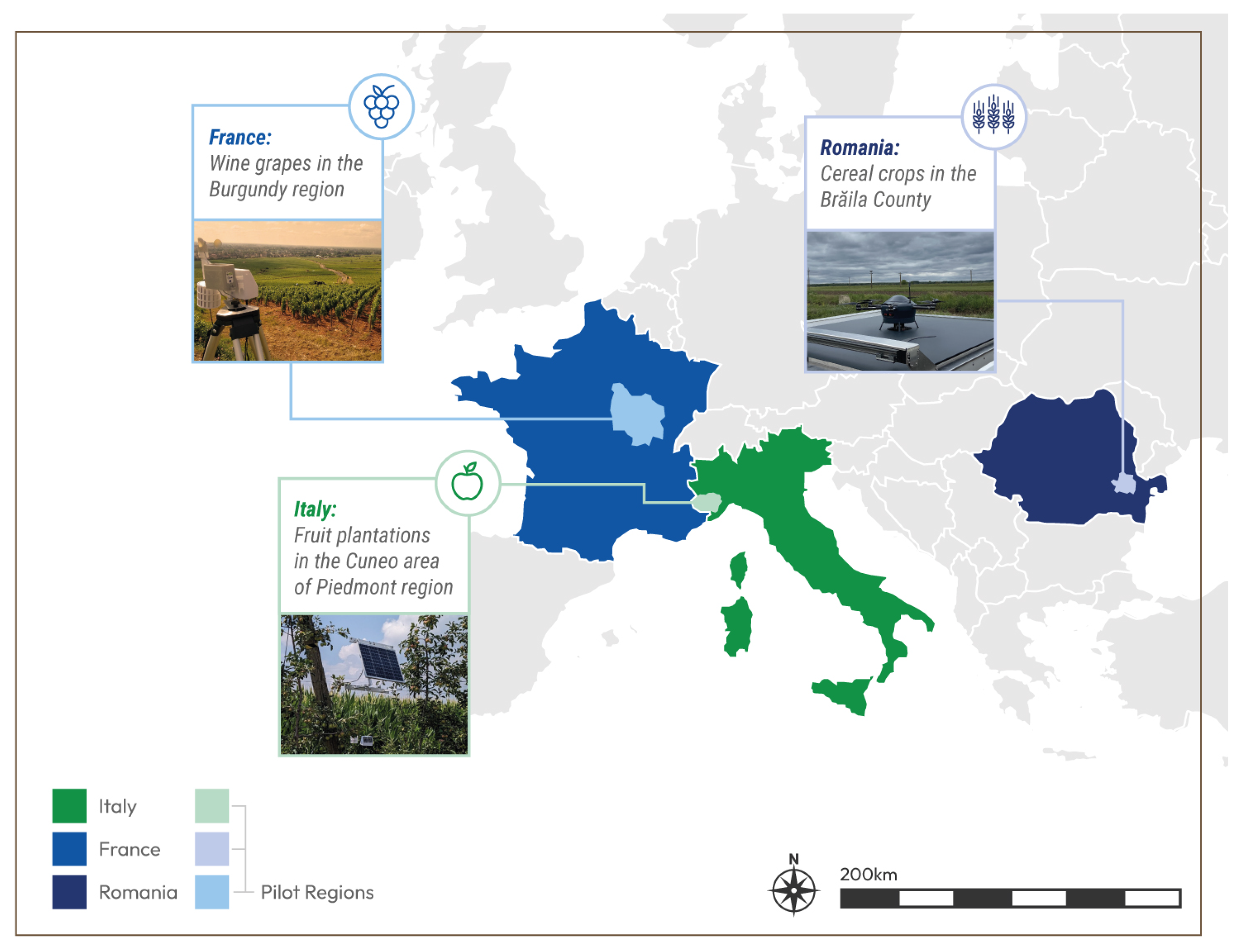
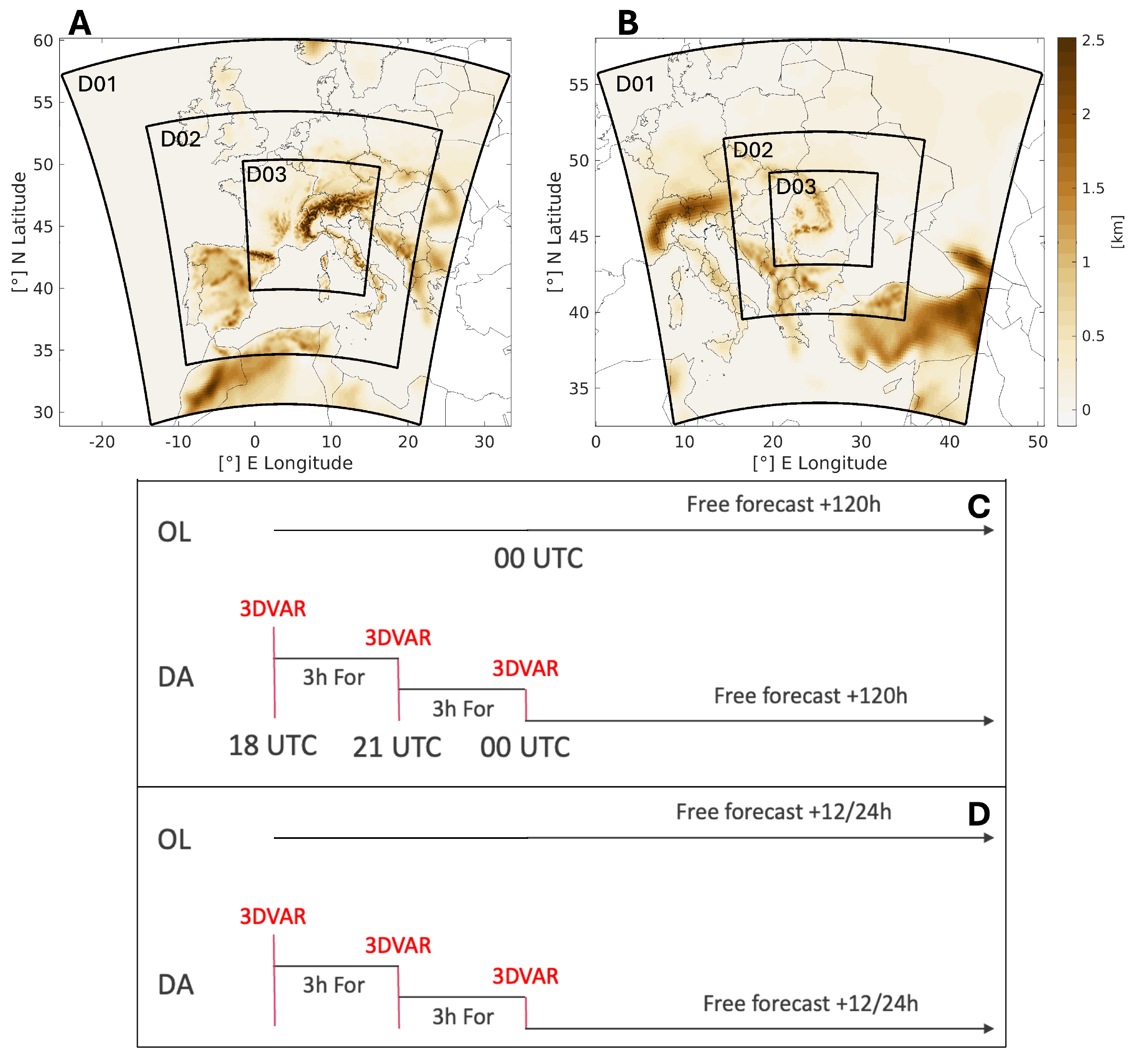

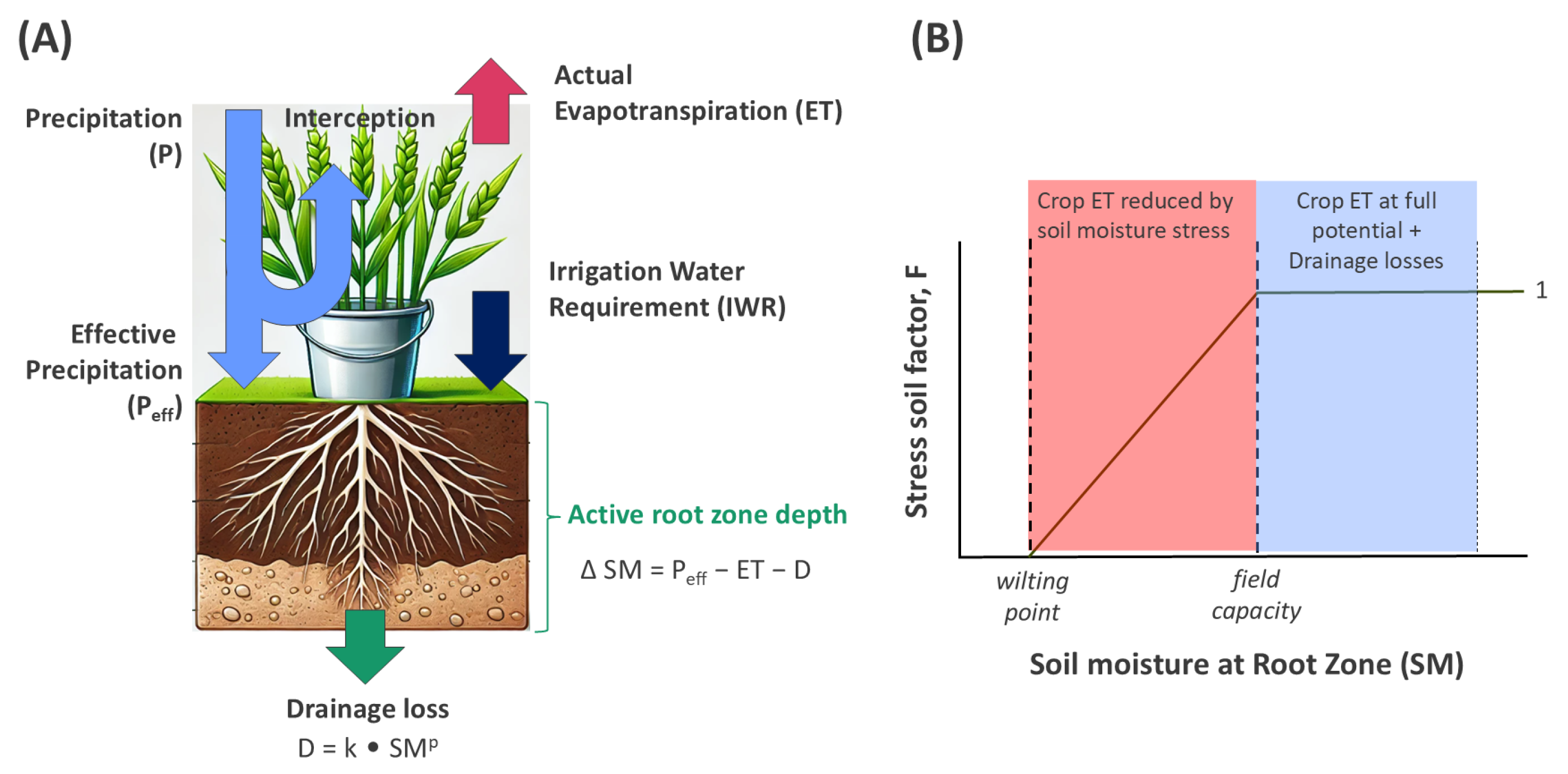
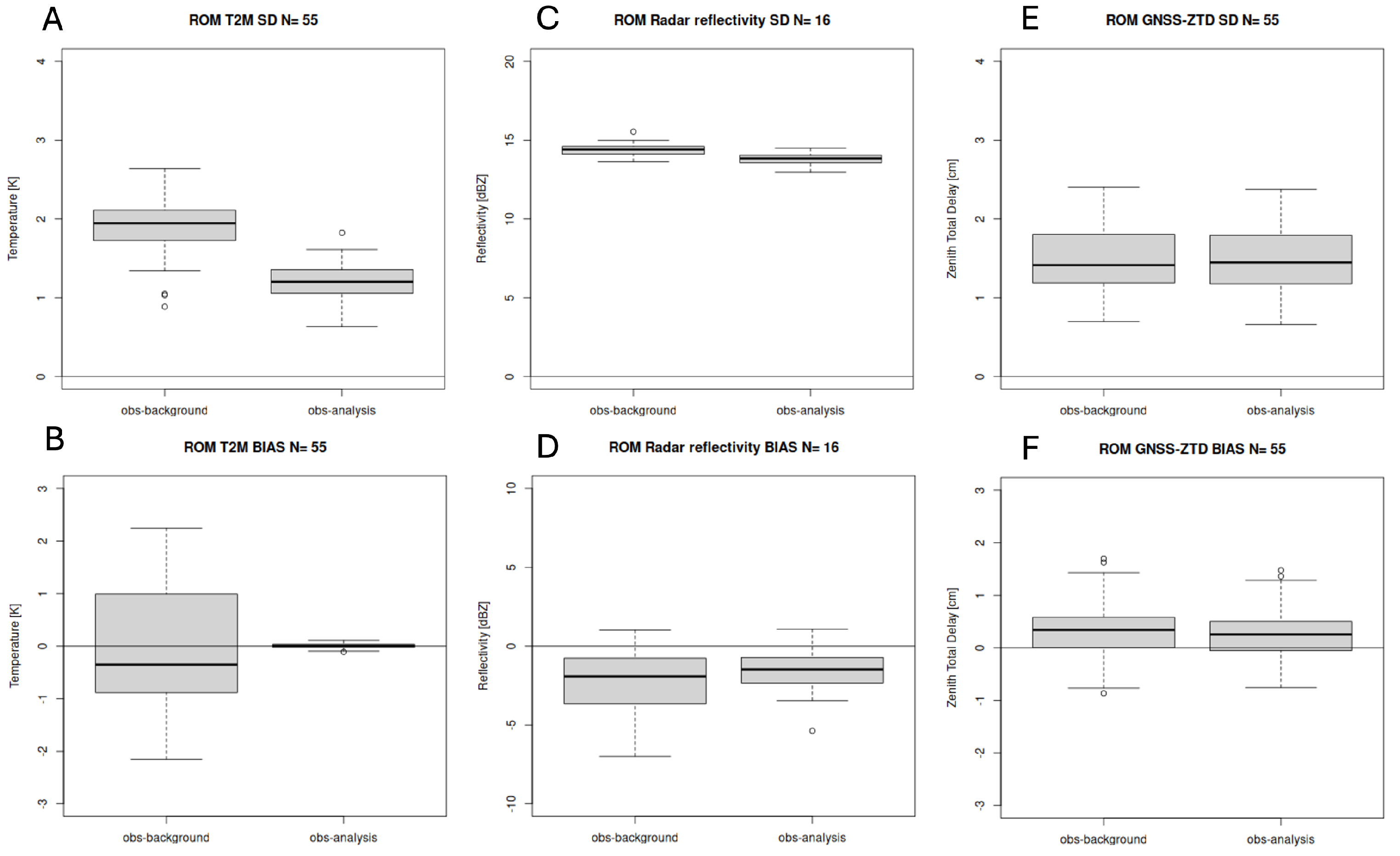
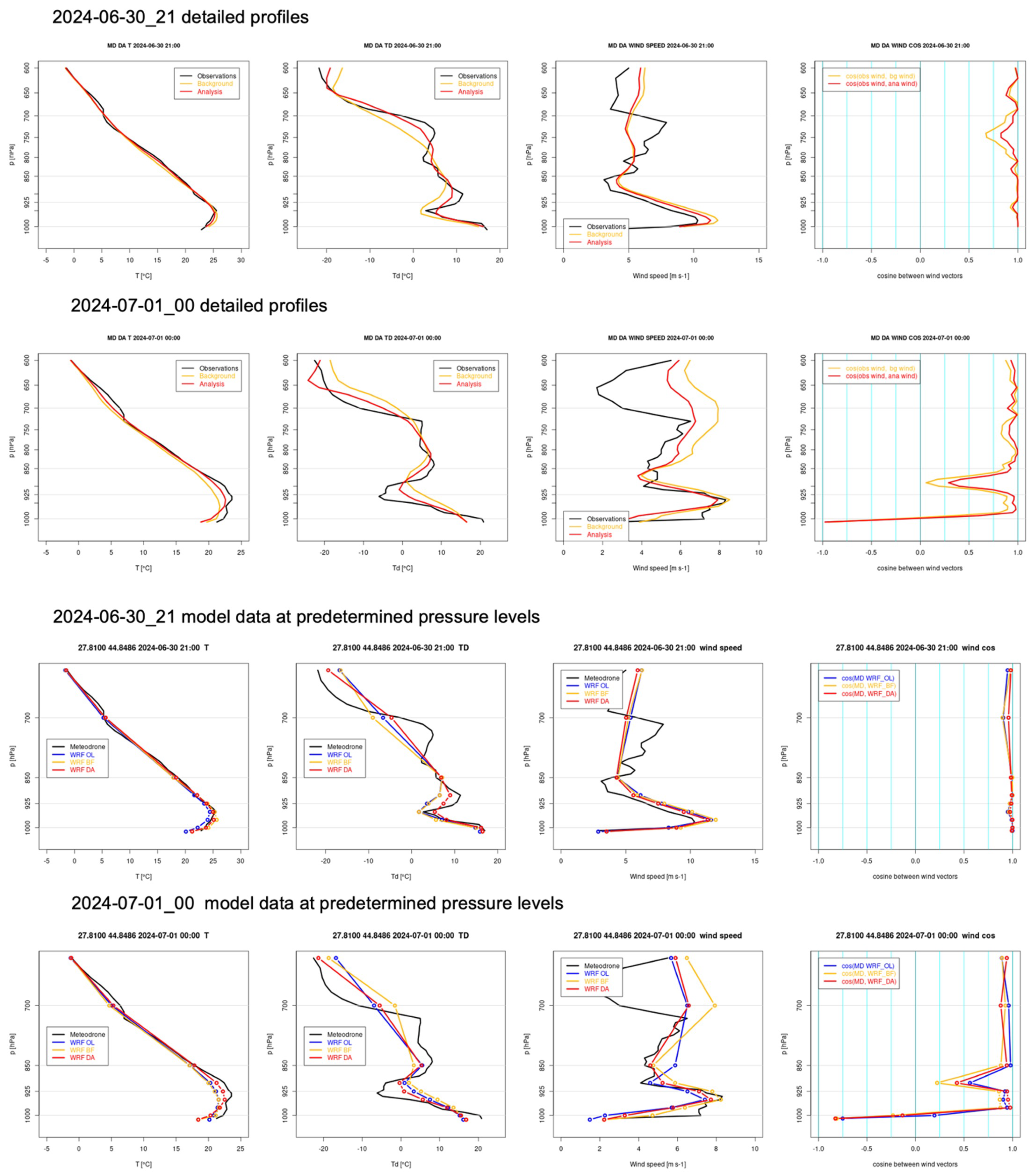
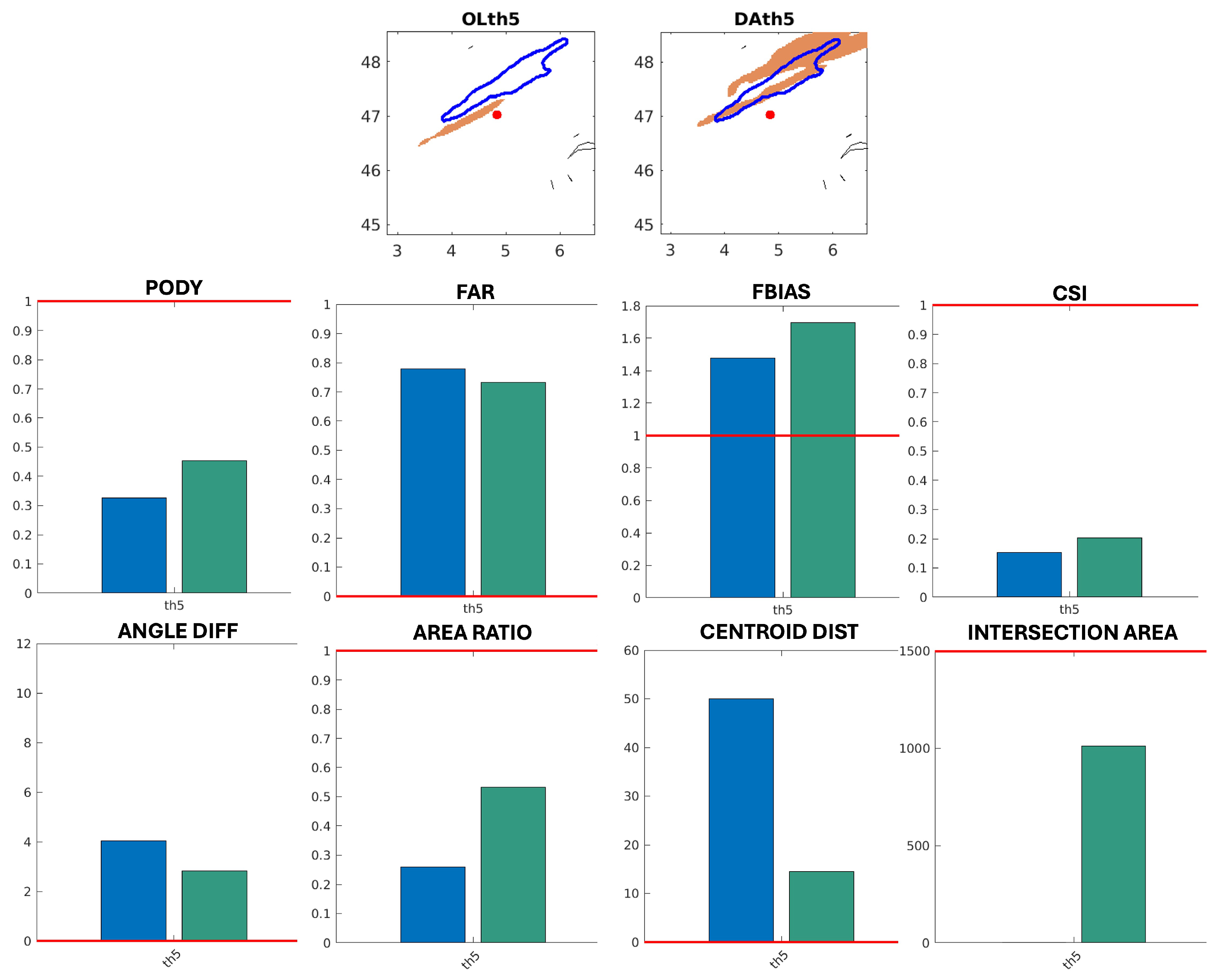

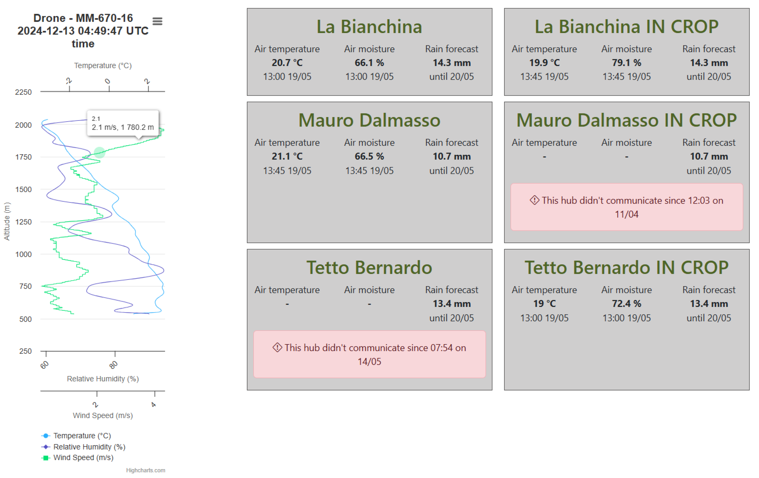
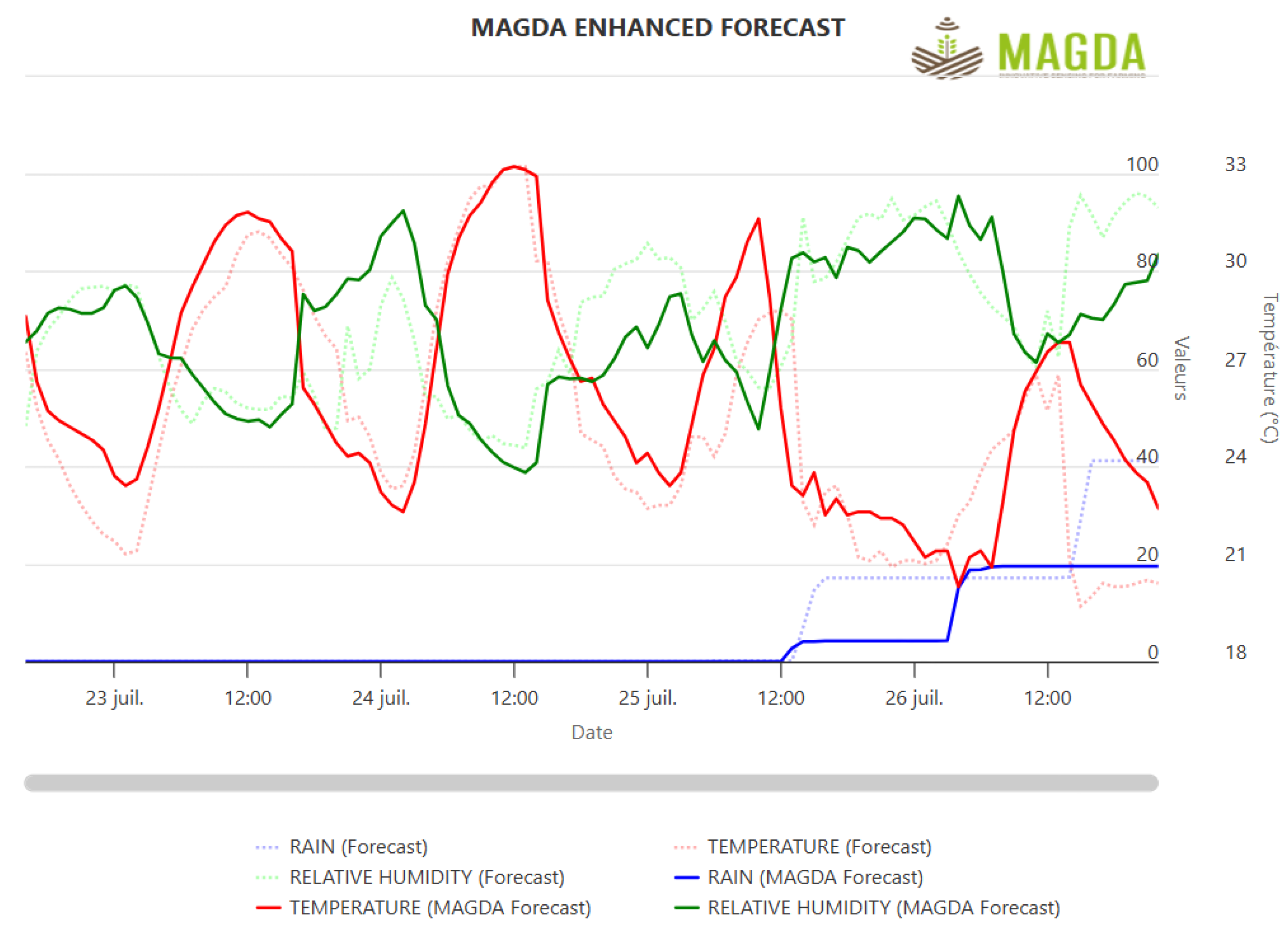
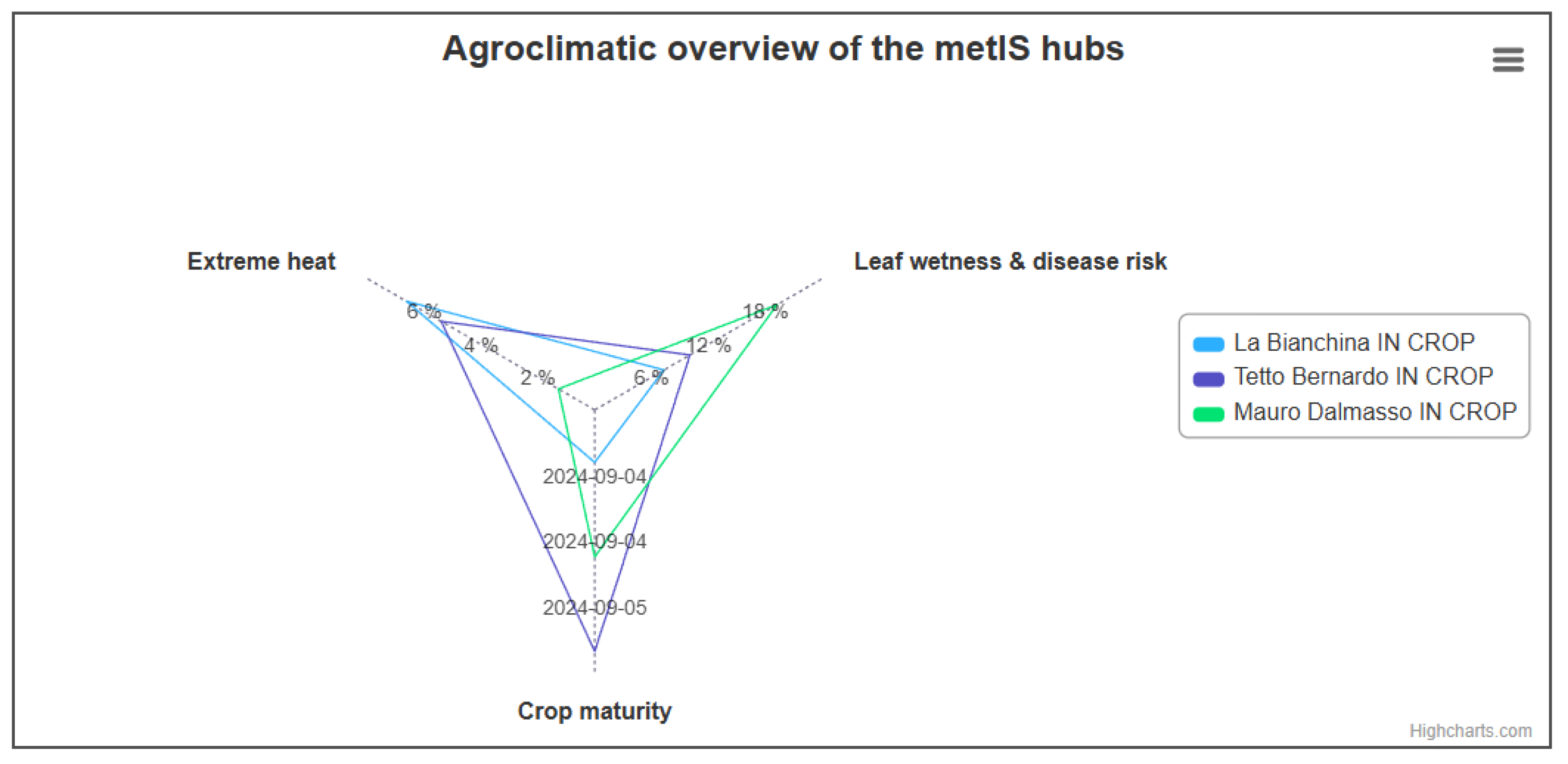
Disclaimer/Publisher’s Note: The statements, opinions and data contained in all publications are solely those of the individual author(s) and contributor(s) and not of MDPI and/or the editor(s). MDPI and/or the editor(s) disclaim responsibility for any injury to people or property resulting from any ideas, methods, instructions or products referred to in the content. |
© 2025 by the authors. Licensee MDPI, Basel, Switzerland. This article is an open access article distributed under the terms and conditions of the Creative Commons Attribution (CC BY) license (https://creativecommons.org/licenses/by/4.0/).