Article

An Assessment of TROPESS CrIS and TROPOMI CO Retrievals and Their Synergies for the 2020 Western U.S. Wildfires

by
Oscar A. Neyra-Nazarrett
1,2,3,
Kazuyuki Miyazaki
2,
Kevin W. Bowman
2,3 and
Pablo E. Saide
1,4,*
1
Institute of the Environment and Sustainability, University of California, Los Angeles, CA 90095, USA
2
NASA Jet Propulsion Laboratory, California Institute of Technology, Pasadena, CA 91109, USA
3
Joint Institute for Regional Earth System Science & Engineering (JIFRESSE), University of California, Los Angeles, CA 90095, USA
4
Department of Atmospheric and Oceanic Sciences, University of California, Los Angeles, CA 90095, USA
*
Author to whom correspondence should be addressed.
Remote Sens. 2025, 17(11), 1854; https://doi.org/10.3390/rs17111854
Submission received: 23 December 2024 / Revised: 13 May 2025 / Accepted: 16 May 2025 / Published: 26 May 2025
(This article belongs to the Section Atmospheric Remote Sensing)

Abstract

:
The 2020 wildfire season in the Western U.S. was historic in its intensity and impact on the land and atmosphere. This study aims to characterize satellite retrievals of carbon monoxide (CO), a tracer of combustion and signature of those fires, from two key satellite instruments: the Cross-track Infrared Sounder (CrIS) and the Tropospheric Monitoring Instrument (TROPOMI). We evaluate them during this event and assess their synergies. These two retrievals are matched temporally, as the host satellites are in tandem orbit and spatially by aggregating TROPOMI to the CrIS resolution. Both instruments show that the Western U.S. displayed significantly higher daily average CO columns compared to the Central and Eastern U.S. during the wildfires. TROPOMI showed up to a factor of two larger daily averages than CrIS during the most intense fire period, likely due to differences in the vertical sensitivity of the two instruments and representative of near-surface CO abundance near the fires. On the other hand, there was excellent agreement between the instruments in downwind free tropospheric plumes (scatter plot slopes of 0.96–0.99), consistent with their vertical sensitivities and indicative of mostly lofted smoke. Temporally, TROPOMI CO column peaks were delayed relative to the Fire Radiative Power (FRP), and CrIS peaks were delayed with respect to TROPOMI, particularly during the intense initial weeks of September, suggesting boundary layer buildup and ventilation. Satellite retrievals were evaluated using ground-based CO column estimates from the Network for the Detection of Atmospheric Composition Change (NDACC) and the Total Carbon Column Observing Network (TCCON), showing Normalized Mean Errors (NMEs) for CrIS and TROPOMI below 32% and 24%, respectively, when compared to all stations studied. While Normalized Mean Bias (NMB) was typically low (absolute value below 15%), there were larger negative biases at Pasadena, likely associated with sharp spatial gradients due to topography and proximity to a large city, which is consistent with previous research. In situ CO profiles from AirCore showed an elevated smoke plume for 15 September 2020, highlighted consistency between TROPOMI and CrIS CO columns for lofted plumes. This study demonstrates that both CrIS and TROPOMI provide complementary information on CO distribution. CrIS’s sensitivity in the middle and lower free troposphere, coupled with TROPOMI’s effectiveness at capturing total columns, offers a more comprehensive view of CO distribution during the wildfires than either retrieval alone. By combining data from both satellites as a ratio, more detailed information about the vertical location of the plumes can potentially be extracted. This approach can enhance air quality models, improve vertical estimation accuracy, and establish a new method for assessing lower tropospheric CO concentrations during significant wildfire events.

1. Introduction

Unlike previous years, the 2020 season generated a record-breaking burned area in the Western U.S., which resulted in strong local, regional, and continental impacts from the smoke emitted [1]. The 2020 season wildfires burned over 10 million acres, which resulted in the largest monthly total Fire Radiative Power over the last 19 years [2]. Climate anomalies were partially responsible for the unusually high wildfire activity and heavy smoke with strong vertical transport [3,4]. Wildfires can generate large amounts of CO due to incomplete fuel combustion happening during biomass burning and due to oxidation of hydrocarbons, making CO a good smoke tracer [5]. Thus, the wildfires of 2020 were a major source of carbon monoxide (CO), resulting in three times larger CO emissions compared to the 2001–2019 average [1].
Satellite retrievals play an essential role in studying global atmospheric composition, as they cover a wide area, complementing the more localized and precise observations of ground-based networks [6]. During the period of global lockdown from COVID-19, satellites remained operational and proved to be an important tool for characterizing the spatiotemporal distribution of gases and aerosols at a global scale [7]. Various satellites have been used to measure CO through the estimation of the radiation they absorb. In the thermal infrared (TIR) spectral regions, these include the Infrared Atmospheric Sounding Interferometer (IASI) [8]; the Tropospheric Emissions Spectrometer (TES) [9]; the Cross-track Infrared Sounder (CrIS) [10,11]; and the Atmospheric Infrared Sounder (AIRS) [12]. Retrieval algorithms typically use optimal estimation approaches to retrieve CO columns from the measured radiances and have shown consistent hemispheric CO variability [13]. The TIR measurements have limited sensitivity to near-surface concentrations in the spectral bands they detect [14]. On the other hand, instruments such as TROPOMI use near-infrared (NIR) channels to derive CO atmospheric columns [15]. In the NIR, TROPOMI is sensitive to the entire column in the troposphere. TIR instruments, such as CrIS, are primarily sensitive to the free lower and middle troposphere above the boundary layer. Using TROPOMI onboard the Sentinel-5P satellite and CrIS onboard the Suomi-NPP satellite, we benefit from their complementary capabilities and their strategic colocation in a tandem orbit on the same satellite train. This offers enhanced synergistic potential and the opportunity for the development of future joint retrievals [16], making them uniquely suitable to our study.
There is limited literature on the joint validation and assessment of the synergistic potential of TROPOMI and CrIS, and there is also a lack of evaluation of these satellite retrievals specifically for strong smoke events. Prior studies have validated CO retrievals from CrIS or TROPOMI by comparing them independently against other satellite datasets [11,13,17,18,19,20], aircraft-based vertical profiles [5,20], and ground measurements [21,22]. These studies generally found that both CrIS and TROPOMI are well correlated with other satellites, airborne data, and ground measurements. For CrIS, comparisons with aircraft profiles showed biases of −0.04% to 0.6% for partial column average volume mixing ratios (VMRs) [11]. As expected, near the surface level, CrIS typically has lower sensitivity, resulting in overestimation in low-concentration conditions and underestimation in higher atmospheric concentration conditions [21], but it can be accounted for with appropriate diagnostics [11]. In multi-satellite instrument comparisons, one study [5] compared TROPOMI CO column data to MOPITT satellite data, finding that TROPOMI CO retrievals over land show an average relative bias of −3.73%, −2.24%, and −3.22% compared to MOPITT’s TIR, NIR, and multispectral products, respectively, and show good agreement in temporal and spatial patterns between them. Another study [20] presented an intercomparison of TROPOMI CO measurements with MOPITT, including validation using vertical profiles from balloon-borne AirCore measurements. It highlighted that TROPOMI can retrieve CO well under both clear and cloudy conditions, with a relative bias and standard deviation of 2.02% in cloudy conditions, after accounting for TROPOMI’s vertical sensitivity to CO. Sha, et al. [23] validated TROPOMI’s CO products over three years using ground-based data from the Total Carbon Column Observing Network (TCCON) and the Infrared Working Group (IRWG) of the Network for the Detection of Atmospheric Composition Change (NDACC), addressing uncertainties in a priori alignment and smoothing. Moreover, TROPOMI retrievals have also been found consistent with atmospheric composition reanalysis [15], further affirming the reliability of TROPOMI CO retrievals.
The concept of “satellite synergy” entails the use of data from multiple satellite sensors to observe attributes of the environment that are not discernible with a single satellite instrument. Joint retrieval, on the other hand, combines spectral radiance measurements from two or more sensors to infer geophysical information, e.g., trace gases, with greater accuracy than either sensor separately. These approaches are based upon optimal estimation, which has been demonstrated to be highly advantageous [12,16,24,25,26,27,28,29,30,31]. One recent study demonstrated the effectiveness of joint retrievals using CrIS-TROPOMI for ozone [24] and theoretically for CO [16]. We study the potential for these synergies for a large wildfire event.
High-intensity wildfire events are an important application of the synergistic capability of TROPOMI and CrIS CO measurements. Our study has two key objectives. First, it aims to understand the underlying differences in the way CrIS and TROPOMI observed CO during megafires to evaluate their synergies. Second, satellite measurements are compared to ground-based reference measurements for cross-validation. This work is organized as follows. In Section 2, we describe the data and method used to homogenize the data from all the instruments. In the Section 3, we present and discuss the results of our study through temporal, spatial, and vertical lenses, and in Section 4, we present the conclusions and future directions of this study.

2. Data and Methods

2.1. Satellite CO Retrievals

In this section, we provide a summary of the features and characteristics of the two satellite CO products we utilized to perform our study. An overview pf the products is provided on Table 1.

2.1.1. CrIS CO

We used CO retrievals from the Cross-track Infrared Sounder (CrIS), a Fourier transform spectrometer (FTS) aboard the Suomi National Polar-Orbiting Partnership (S-NPP) satellite (also referred to as NOAA-19), which has been providing quasi-global daily data since 2015. The data of this instrument were obtained from the NASA TRopospheric Ozone and its Precursors from Earth System Sounding (TROPESS), which employs optimal estimation leveraging the Tropospheric Emission Spectrometer (TES) algorithm [9]. The TROPESS CO CrIS algorithm has been well validated and is in excellent agreement with other sensors [11]. The data were produced operationally at a 0.7-degree resolution to save computational costs. We tested the impact of the resolution on our data by comparing its consistency with reprocessed data of a higher resolution (0.25 degree) for the period of 11–15 September 2020, which displayed the highest CO concentrations in the fire season. We analyzed daily averages for the same geographical region at both resolutions and found that using 0.7-degree resolution provided similar results, as shown in Figure A1.

2.1.2. TROPOMI CO

The other satellite instrument utilized was TROPOMI. It is an imaging spectrometer on board the Sentinel 5P Satellite from the European Space Agency [15]. TROPOMI has a wide swath width of 2600 km, which provides quasi-global daily coverage. It measures radiances in the ultraviolet, visible, and solar-reflected infrared ranges [20]. Its total CO column values are obtained from measurements of infrared radiation in the 2.3 μm spectral band. Both CrIS and TROPOMI have the ability to retrieve CO over land in both clear and cloudy conditions [11,33]. This capability is due to their ability to retrieve parameters such as cloud height and optical thickness concurrently with trace gas columns. The recent operational changes to the Copernicus Sentinel-5P have enhanced the resolution of TROPOMI, providing data at approximately 7 × 5.5 km2 since August 2019, which has been beneficial for our study that utilizes 2020 data.

2.2. Reference Data

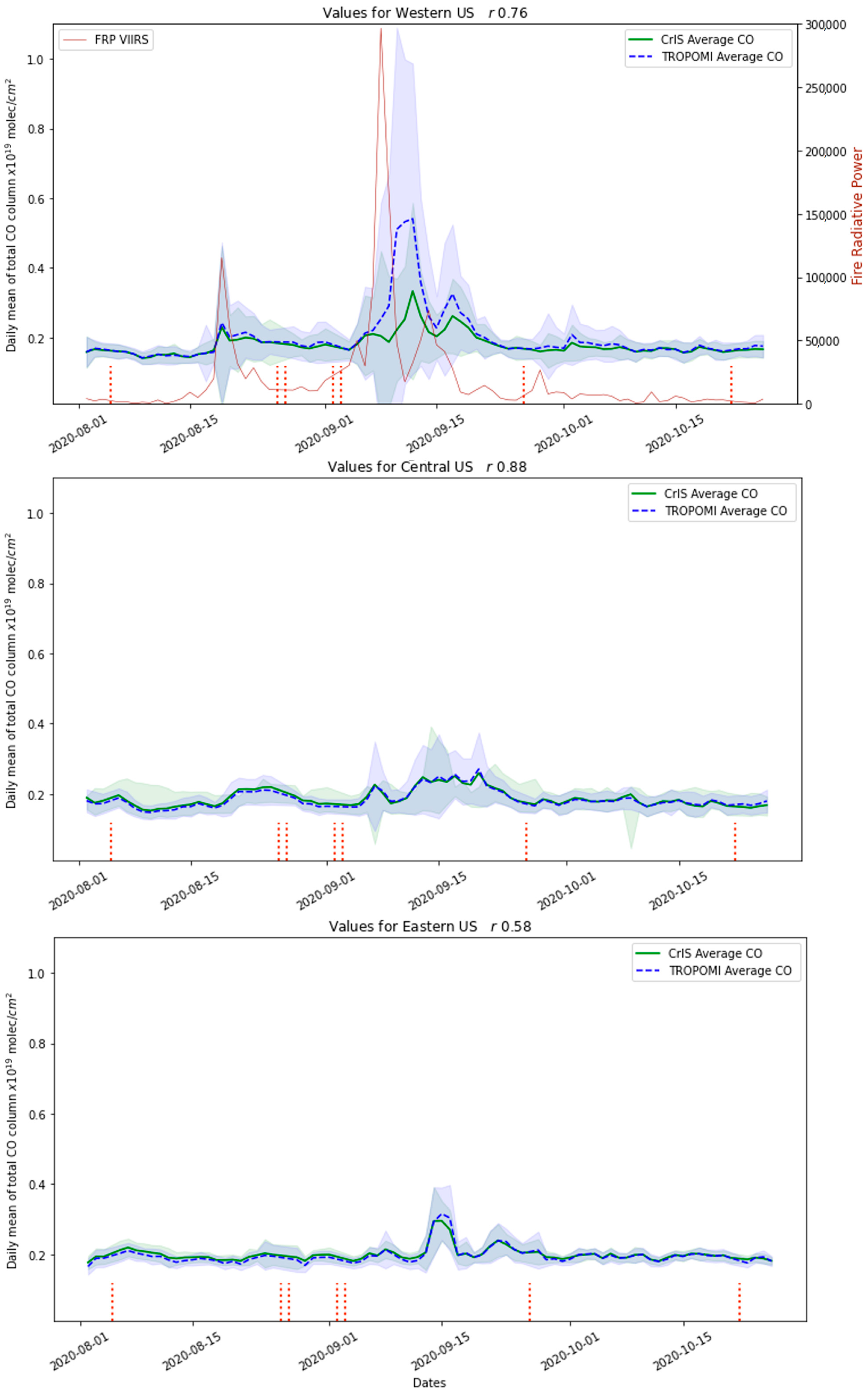
2.2.1. Satellite Fire Radiative Power Retrievals from VIIRS

To track fire activity, we used Fire Radiative Power (FRP) data from the Visible Infrared Imaging Radiometer Suite (VIIRS) instrument carried by the Suomi NPP Satellite. Such an instrument offers the advantage of providing daily globally active fire data [34]. Specifically, we used S-NPP VIIRS with a pixel resolution of 375 m-pixel [35]. Like CrIS, VIIRS is on the S-NPP satellite, and, thus, their measurements are collocated and share the same orbital characteristics, passing over the equator at around 1:30 local time during the descending orbit and at approximately 13:30 local time during the ascending orbit. The Fire Radiative Power (FRP) metric quantifies the total amount of radiant energy released by the fire and is expressed in megawatts (MW) at the pixel level. The product (VNP14IMGTDL_NRT) is available at the Fire Information for Resource Management System (FIRMS) database.
To quantify fire activity, we employed a cumulative estimation of Fire Radiative Power (FRP) using aggregated data over both time and space. We summed up the FRP emitted by fires across broader geographic segments, capturing the total energy output over the study period. The majority of fire activity during this season occurred in the Western U.S., so we limited the FRP data analysis to this region.

2.2.2. Ground-Based TCCON CO Measurements

The TCCON Network is integrated by a ground-based Fourier transform spectrometer (FTS), and it is currently the state-of-the-art reference measurement to validate total column measurements through remote sensing [36]. The FTSs in the TCCON network use direct solar absorption spectra in the NIR spectral range to obtain column-averaged measurements of atmospheric constituents, such as CO2, CH4, and CO [23,37]. TCCON has been effectively used to validate trace gas data products from satellite instruments such as GOSAT, OCO-2, MOPITT, and SCIAMACHY [23].
We use data from three stations located in the states of Oklahoma, California, and Wisconsin (Lamont, Pasadena, and Park Falls, respectively), as outlined in Table 2. These locations were selected to enable a West, Central, and East comparison and to observe how plumes generated in the West evolved chemically as they moved eastward. To evaluate CO column measurements from satellites, we used the official TCCON XCO product, in which wet mole fractions are converted to columns, as outlined in Section 2.4 The TCCON data were obtained directly from https://tccondata.org/ (last access: 18 January 2023).

2.2.3. Ground-Based NDACC-IRWG CO Retrievals

We used data from the Boulder station of the Network for the Detection of Atmospheric Composition Change (NDACC), as provided by Ortega and colleagues. NDACC encompasses more than 20 stations, each outfitted with high-resolution Fourier transform spectrometers. These devices measure solar absorption spectra within the mid-infrared (MIR, 2–14 μm) spectral range [40].
The NDACC retrieves CO measurements in the MIR spectra using three narrow spectral windows in the CO fundamental absorption band [13,21,41]. Because of its rigorous calibration and quality control procedures, long-term and consistent data record, high-quality data, global coverage, traceability to SI standards, and open access to data, NDACC has been extensively used to validate satellite data in prior studies [13,21,22,42,43,44].

2.2.4. CO Vertical Profiles from AirCore

We acquired vertical profiles of CO concentration obtained through the use of the balloon-based AirCore instrument [20,45,46]. Data were acquired for two specific dates: 12 August 2020 and 15 September 2020, with launches conducted in Boulder, Colorado.
The AirCore data were obtained directly from the NOAA Global Monitoring Laboratory site (http://gml.noaa.gov/ccgg/arc/tmp/arcrepo_34Twm7/NOAA_AirCore_data_v20210813.zip, last accessed: 5 January 2022).

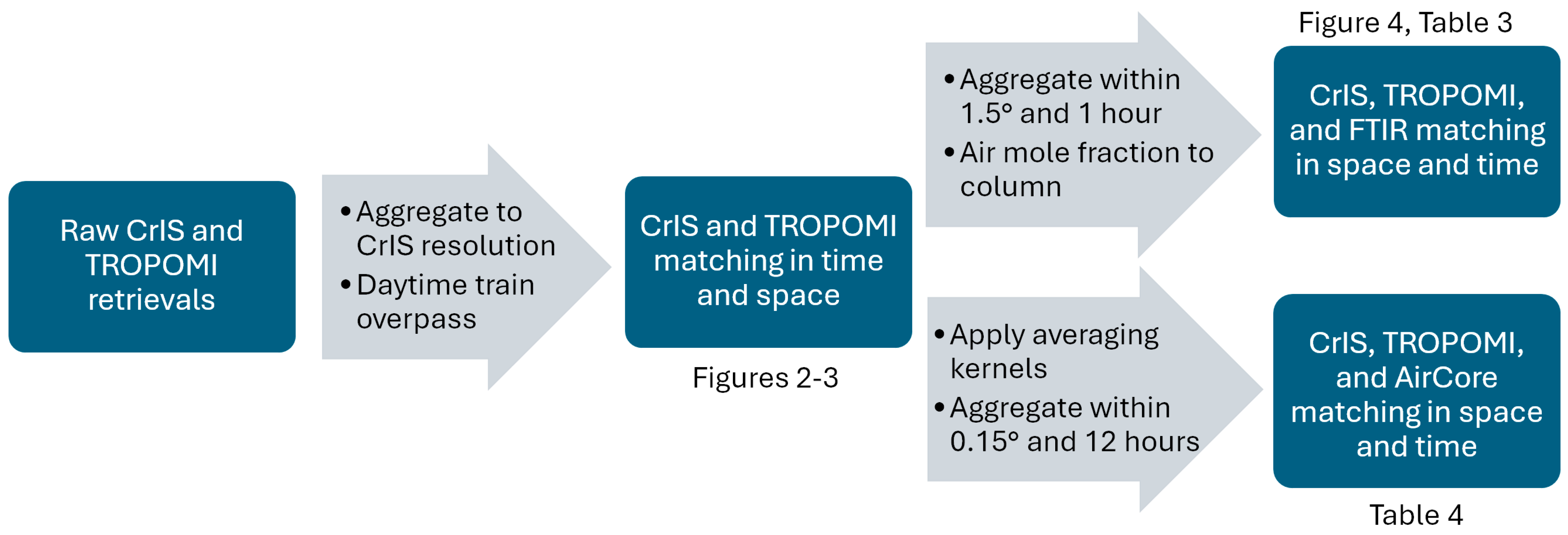
2.3. Collocation of Datasets

To jointly assess and validate CrIS and TROPOMI CO measurements, we matched retrievals in space and time and compared CO column densities obtained from both to each other and to reference assets, as described in the following subsections. A diagram summarizing the matching of the datasets is shown in Figure 1.

2.3.1. Temporal Colocation of Satellites

We used temporal colocation to match TROPOMI and CrIS data, following the methods used in previous studies [47] to ensure sensors observe a similar location at a similar time. Fortunately, S-5P (hosting TROPOMI) and S-NPP (hosting CrIS) are both in a tandem orbit, and, therefore, one satellite overpasses the Earth right before the other, with an equatorial crossing time of roughly 1:30 p.m. local time and an overpass time difference of less than 5 min [48]. Because both sensors are in the same train and have similar swaths, measurements that meet the temporal condition will likely have a match for the spatial criterion.
Despite being in the same train, collocating TROPOMI and CrIS data creates difficulties due to their heterogeneous nature and the spatial and temporal constraints that must be met. To address this, we developed a colocation approach that simplifies data processing. We used TROPOMI data over the continental United States, filtered and organized based on satellite overpass times, and then temporally matched with CrIS daytime retrievals. Hence, we obtained measurements that are both temporally and spatially homogeneous, albeit at varying resolutions.
To ensure the reliability of the data, we established additional filters. We only used daytime data for CrIS (TROPOMI data are daytime only), and quality filters with a minimum threshold of 0.5 were used for each of the two retrievals, “qa_value” for TROPOMI and “Quality” for CrIS, following the recommendations in the data user manuals [32,49].

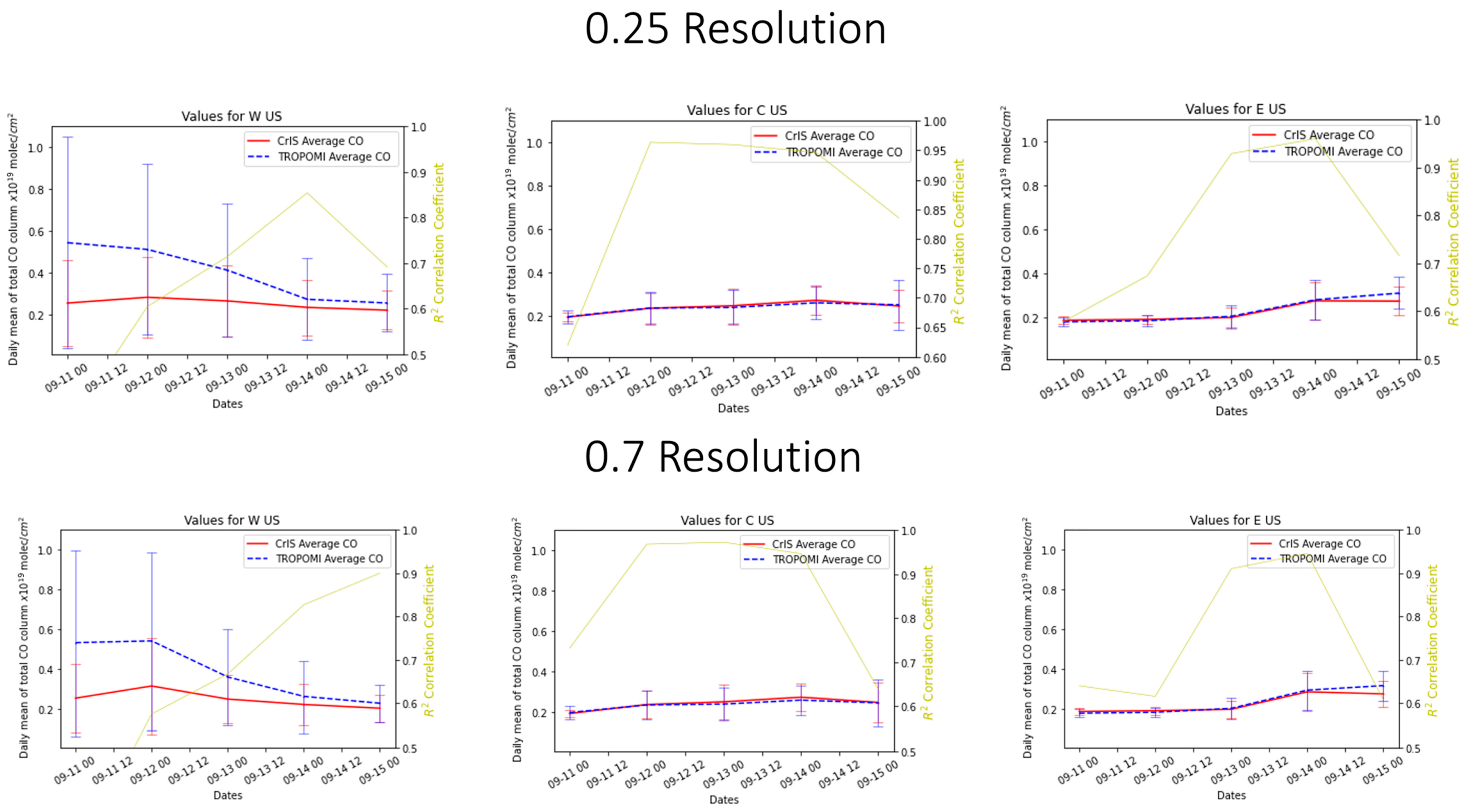
2.3.2. Re-Gridding of Satellite Data

After performing temporal and spatial colocation of the data, we adjusted the resolution to ensure compatibility between the CrIS and TROPOMI datasets. Since CrIS pixels (15 × 15 km collected at 0.25-degree bins) have a larger size and different resolution than TROPOMI pixels (7 km × 3.5 km), TROPOMI was regridded to the CrIS grid by using the center of each CrIS pixel, drawing a square of 0.1° per side around it, and averaging the TROPOMI pixels, the center of which falls within the square. The dataset was then stripped of all CrIS pixels that did not have associated TROPOMI pixels to only keep paired pixels.

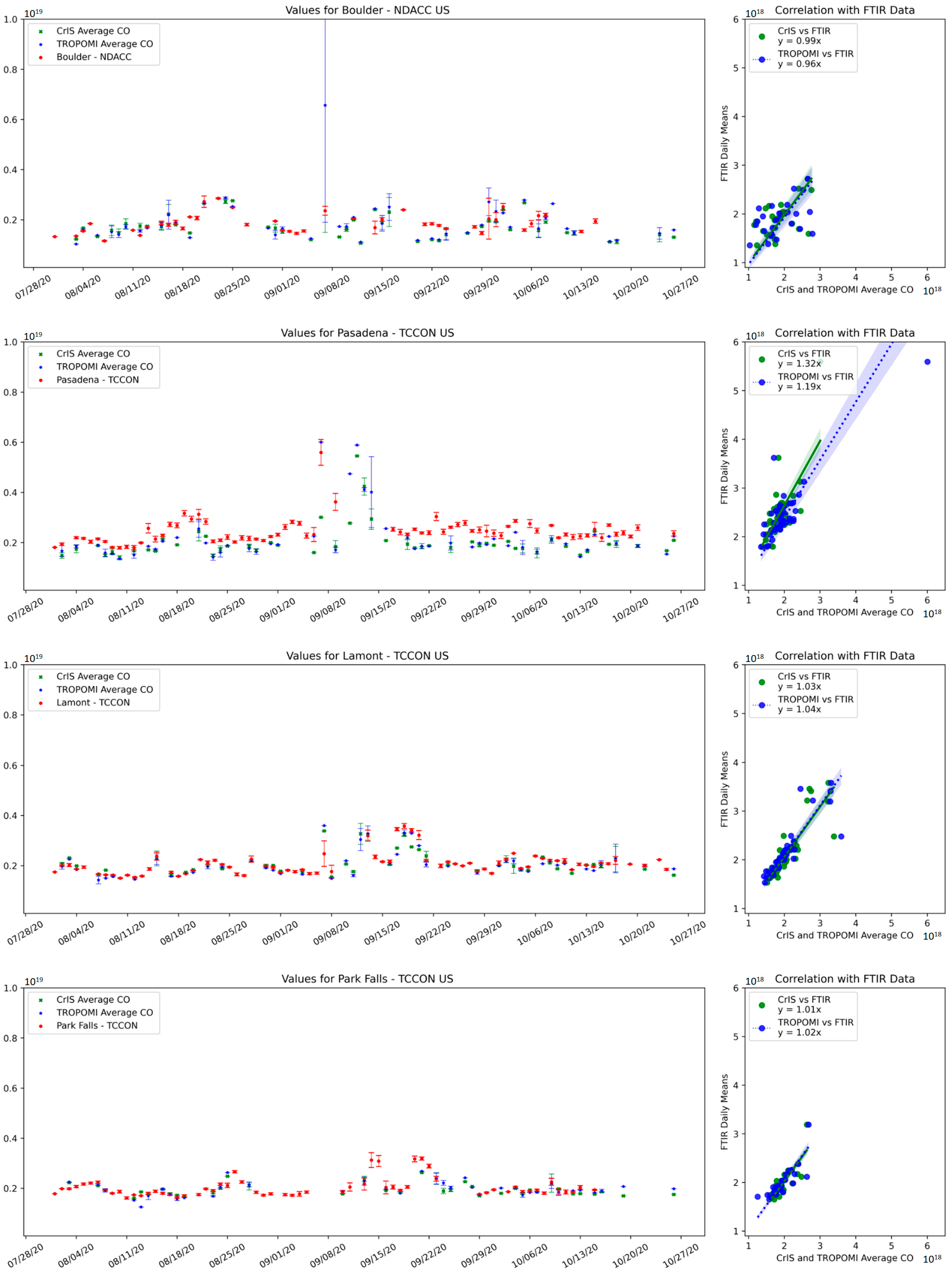
2.4. FTIR Colocation

To verify the accuracy and consistency of our data, we conducted a spatial colocation process whereby we compared the satellite measurements with the ground-based FTIR measurements. For each day, we chose the CrIS and TROPOMI homogenized observations that corresponded to the position of the ground-based reference data. By centering on the FTIR locations, we selected matching daily satellite data within a square centered at the site with a side of 1.5°.
Once we successfully achieved spatial colocation between satellite data and FTIR, we calculated the spatial averages by obtaining an average daily measurement for CrIS and TROPOMI. However, we had multiple daily measurements for FTIR at this stage. Therefore, we filtered the FTIR data to align them temporally with the timing of the satellite retrieval overpassing times, averaging all FTIR retrievals for the corresponding hour. Standard deviation was also calculated and is reported in the plots as error bars. No outliers were removed from the statistics, except for a single day (19 August) on the Boulder station, likely associated with cloudiness (see Section 3.2.1 for details).
The CrIS and TROPOMI column results were then compared directly to the Boulder NDACC data product, as it already provides column estimates [38]. Yet, to align TCCON with the other measurements, units were converted from column-averaged dry-air mole fractions to dry column through a methodology closely aligned to that of previous studies [23,47,50,51]. We calculated the total dry CO column using a method similar to existing methodologies [52]. Specifically, we converted the surface pressure (Ps) from atmospheres of wet air into molecules per cm2, obtained at the lowest vertical level of the prior total air column. Subsequently, we estimated the proportion of this column that represents dry air to determine the dry CO column. This is described by the following equations:
C o l u m n _ C O D r y = C o l u m n _ A i r w e t X C O P e r c e n t _ D r y
which is equivalent to
C o l u m n _ C O D r y = P r i o r _ P S S u r f a c e M W A i r X C O 1 X H 2 O X C O
where
C o l u m n _ C O D r y = the total dry column of carbon monoxide (CO), calculated as the number of CO molecules per cm2.
C o l u m n _ A i r w e t = the total air column, including water vapor, in molecules per cm2, derived from the surface pressure of wet air.
X C O = the volume mixing ratio of CO (unitless).
P e r c e n t _ D r y = the fraction of the total column that represents dry air (unitless), accounting for the removal of water vapor content.
P r i o r _ P S S u r f a c e = the surface pressure of wet air, measured in atmospheres (atm).
M W A i r = the molecular weight of air, accounting for its composition (g mol−1).
X H 2 O = the volume mixing ratio of water vapor in the atmosphere (unitless).

2.5. Collocation to AirCore Data

Besides providing CO columns, TROPOMI and CrIS retrievals include the Averaging Kernels, which provide information on the sensitivity of the measurements to the different pressure/altitude bins, and can be applied to observed or modeled vertical profiles to estimate what the CO column would be under those conditions if it was observed by each satellite instrument [15,49]. We estimated the total CO column from the AirCore data by applying the Averaging Kernels (AKs) of colocated CrIS and TROPOMI retrievals to the AirCore CO profiles. For TROPOMI, we used AK in units of meters derived from a first-order Tikhonov–Phillips regularization on a logarithmic scale [53,54] resulting in a CO column comparable to TROPOMI CO columns. For CrIS, we used Averaging Kernels derived from Optimal Estimation as ln (VMR), resulting in smoothed profiles that take into account the vertical sensitivity of this instrument [11]. The smoothed CO profile was then used to calculate a CO column to compare against the CrIS CO columns.
The colocation criteria required that measurements from the two devices be collected within a time range of 12 h or less and within a geographical proximity of 0.15 degrees or less. We selected a geographical proximity of colocation finer than the 1.5° used when comparing FTIR measurements. As for the day analyzed (Sept 15, see Section 3.2.2), there were strong spatial gradients in the CO retrievals, with the closer proximity being a better representative of smoke. For both CrIS and TROPOMI, we took the average of pixels that satisfied these colocation conditions. To reduce colocation errors, we used high-resolution data processed at a granularity of 0.25 degrees for CrIS and standard high-resolution data for TROPOMI.
We conducted a vertical regridding [47] of the AirCore data to match the levels of CrIS and TROPOMI, using pressure as a reference. Given the initial difference in vertical levels—with AirCore at 521 levels, TROPOMI at 50, and CrIS at 67—this regridding process ensured alignment with TROPOMI and CrIS. It also allowed for the application of Averaging Kernels, harmonizing the AirCore profile with the respective satellite measurement profiles.
In terms of uncertainties of the comparisons, the largest uncertainties are expected to come from time colocation, spatial representativeness (as AirCore is a profile, while satellites measure over their footprints), and uncertainties in the retrievals. AirCore measurements have an accuracy of <10 ppb [55], which is low compared to the values observed (free-tropospheric background of 70–100 ppb with plume peaking > 300 ppb) and, thus, likely do not contribute substantially to the uncertainty of the analysis.

3. Results and Discussion

3.1. Satellite Synergy Evaluation

We compared CO columns from CrIS and TROPOMI after applying the colocation method described earlier (Section 2.3). Figure 2 shows the spatial maps of CO columns observed by the satellites on 12 September 2020 for the continental U.S., which displayed one of the highest daily average CO measurements of the entire fire season. We focused on three regions: the Western, Central, and Eastern U.S. (regions shown in Figure 2). The results show, as expected, that concentrations in the Western U.S. were much higher than in the other two regions. Near the fires, TROPOMI often showed larger values than CrIS (slope of 1.52), and there was large spread in the scatter plots (R2 of 0.32) going from values close to the 1:1 line up to very large TROPOMI CO columns relative to CrIS, which suggests strong CO abundances in the boundary layer. On the other hand, TROPOMI and CrIS retrieval values were generally similar at locations downwind from the fires, with fit and slope remarkably close to unity for the Central and East regions (0.96–0.99) and tighter correlation (R2 of 0.96 and 0.44 for Central and Eastern regions, respectively). This suggests that the TIR and NIR bands provide consistent information about CO when the abundances are localized to the free troposphere, where both instruments are equally sensitive.
The divergence between TROPOMI and CrIS CO close to the fires is explained by the fact that a significant fraction of CO (~50% on average for this day) was present in the lower troposphere, where CrIS has less sensitivity [9,11,16,24]. As for the Central and Eastern U.S., the slopes close to unity imply that the plumes were mostly lofted in the free troposphere.
Figure 3 displays the daily average concentrations for CrIS and TROPOMI in the three regions of interest, including the standard deviation of such measurements for each given day. Such analysis is further complemented with FRP measurements, which were included exclusively for the Western region, given that the majority of the fire activity occurred in this region, and the majority of CO in the Central and Eastern regions was transported from the Western region.
The temporal analysis shows that the Western region experienced much higher average CO concentrations than the Central and Eastern regions of the U.S. Figure 3 further demonstrates that TROPOMI saw on average higher concentrations than CrIS (up to a factor of 2 higher on 11 September) during and following days with higher FRP in the Western U.S. until about 20 September, when values of both instruments converged. This is of particular relevance for the first three weeks of September, for which time TROPOMI shows not only a much higher daily average than CrIS but also a much higher variability. This again implies that for the most intense period, a large fraction of the smoke might have been close to the surface, where CrIS has low sensitivity.
The CrIS and TROPOMI measurements were slightly delayed relative to FRP, as demonstrated by the CO peak for the Western U.S. In fact, the peak CO columns appear a couple of days after the days with higher FRP, and when FRP had the largest decline from its peak. This shift in the peak is likely due to FRP retrievals peaking when the fires reached their maximum activity and smoke accumulated in the planetary boundary layer. Also, as shown in Figure 2, some of the smoke was transported over the ocean and recirculated, which increased the residence time in the region and contributed to the shift.
When the delay of CrIS relative to TROPOMI during the more extreme period (6–15 September) is further evaluated, it can be observed that increases in CrIS retrievals sometimes occur with 1–2-day delays compared to TROPOMI. These delays could be explained by an accumulation of CO in the boundary layer and then subsequent ventilation into the free troposphere, where CrIS is sensitive. Hence, when there is a delay in CrIS matching TROPOMI CO retrievals, it could mean that a larger amount of CO is remaining in the lower troposphere. Conversely, on other days, TROPOMI and CrIS peak at the same time, and the column amounts are closer, which could mean that a substantial amount of CO has moved to the free troposphere, and the near-surface concentrations have substantially diminished. These variations should reflect changes in various factors, including synoptic weather patterns, local atmospheric stability, and the presence of pyro-convection.
In contrast to the Western U.S., CrIS and TROPOMI daily averages track closely for the Central and Eastern U.S. (Figure 3, bottom panels). This agreement implies that a large fraction of the smoke plume was transported through the free troposphere, and thus, both instruments captured it similarly.

3.2. Evaluation Using Ground-Based and AirCore Data

In this section, we compare satellite data against ground-based reference measurements to illustrate and validate our findings. The temporal and spatial variations are compared against those of the TCCON and NDACC stations. The vertical sensitivity of the satellite products is assessed using the AirCore observations.

3.2.1. FTIR/Satellite

Satellite measurements of CO show close agreement with the observations from TCCON and the NDACC at Boulder, Park Falls, and Lamont (Figure 4), with Normalized Mean Bias (NMB) and Normalized Mean Errors (NME) typically below 24% and 32%, respectively, for all the four sites (Table 3). When the satellites were compared to FTIR, it was impressive to observe that CrIS and TROPOMI demonstrate an underestimation of CO columns by approximately 3–4% while maintaining agreement with each other within a margin of about 1%. However, when Pasadena is compared to FTIR, Pasadena appears as an outlier. While the satellites exhibited rapid temporal variations that are consistent with the TCCON observations. (r = 0.74 for CrIS and 0.88 for TROPOMI), they showed lower mean concentrations, which are also reflected in the slope (~1.19 and 1.32, as shown in Figure 4). This inconsistency aligns qualitatively with the existing literature on the subject [23]. The likely cause of the discrepancy between the TCCON and satellite instruments is the site’s location in a major urban basin in Los Angeles, which is continuously affected by the urban plume and is only partially captured by satellites. The plume is diluted in the satellite data, as it includes regions outside the basin.
As shown in Figure 4, there were a limited number of TCCON data retrievals between 9 September and 22 September 2020 for the Pasadena site. However, one example is available for 7 September in Pasadena, where TROPOMI retrievals are within the variability of TCCON, which shows large values (0.5–0.6 × 10¹⁹ molec/cm2), while CrIS is substantially lower (~0.35 × 10¹⁹ molec/cm2). This corroborates the conclusion that TROPOMI captures most of the column, which seems to have a large fraction close to the ground, as CrIS shows much lower values.
The limited number of TCCON data retrievals between 9 September and 22 September was primarily due to the observatory shutting down because of ash from a nearby fire (Bobcat). This situation was exacerbated by the COVID-19 emergency’s measurement constraints. Despite the difficult circumstances, satellites were able to continue functioning and gathering crucial data.
In Boulder, both TROPOMI and CrIS detected an outlier on 19 August, with values of 0.65 × 10¹⁹ and 1 × 10¹⁹ molec/cm2, respectively (excluded in Figure 4). However, the NDACC data for the same day showed much lower CO values (0.2 × 10¹⁹ molec/cm2). While the large satellite CO columns might have been influenced by the regional smoke and nearby fires, NDACC could have missed it, given that it was a cloudy day. This highlights how cloud cover can obscure ground-based measurements and hinder the detection of smoke, which could also be the case for other stations when the plume is already uplifted. To avoid biasing our estimations, the correlation calculations do not include this outlier.

3.2.2. AirCore/Satellite

There were two dates for which AirCore retrieved vertical profiles for the period of this study. These were 12 August 2020 and 15 September 2020. Since the fires ignited with higher intensity during September, the profile retrieved on 15 September 2020 shows an elevated smoke plume reaching 320 ppm CO and distributed between 7 and 10 km and relatively clean lower troposphere otherwise (70–120 ppm). In contrast, for 12 August, there was no clear evidence of a smoke plume (not shown). This is consistent with the Boulder NDACC site (similar location), as 9/15 shows enhanced columns ~2 × 10¹⁸ molec/cm2 that both satellites captured well (Figure 4). CrIS, TROPOMI, and the corresponding AirCore CO column estimates all show similar values for this day (Table 4), with AirCore estimates being slightly lower. This discrepancy could be attributed to the fact that AirCore is a balloon-based instrument that begins measuring once it reaches a specific altitude (~2.5 km in this case), making it unable to capture the full atmospheric profile down to the surface, and also due to time differences, as AirCore profiles are launched around noon local time versus the afternoon overpass of S-NPP and S5-P.
Considering TROPOMI’s enhanced sensitivity across the vertical distribution of CO, particularly near the surface, and CrIS’s high sensitivity in the lower and middle free troposphere but reduced effectiveness near the surface, using a ratio of CrIS to TROPOMI column measurements emerges as a promising method for determining the vertical placement of CO and other gases and aerosols associated with smoke. This approach capitalizes on the strengths of both instruments.

4. Conclusions and Future Directions

To understand the differences in how CrIS and TROPOMI detected carbon monoxide levels during the 2020 wildfires, we evaluated how satellite measurements compared against ground-based references to better understand their spatial, temporal, and vertical differences.
The differences between CrIS and TROPOMI satellite retrievals near the fires and downwind were captured by contrasting data from the Western U.S. with those from the Central and Eastern regions. While there was a good correlation between TROPOMI and CrIS measurements far from the source regions, there were differences in the satellite retrievals closer to the fire, reflecting near-surface CO accumulation. This is consistent with theoretical calculations of the Averaging Kernels for CrIS and TROPOMI [16,24,56]. Given the synergies between these products, future work should move toward operational implementation of joint TROPOMI-CrIS retrievals that provide further information on the vertical distribution of smoke.
A significant difference in average CO concentrations between the Western U.S. and the Central and Eastern regions was found during periods of high Fire Radiative Power (FRP). Particularly in the first three weeks of September, TROPOMI consistently reported higher concentrations than CrIS in the Western U.S., with daily average values up to a factor of 2 times higher, suggesting substantial CO abundances near the surface, where CrIS has lower sensitivity. Meanwhile, the Central and Eastern U.S. closely tracked daily averages between CrIS and TROPOMI, indicating a similar capture of smoke transport through the free troposphere by both instruments. Interestingly, both CrIS and TROPOMI measurements exhibited a delay relative to FRP, with the CO peak appearing a few days after the peak FRP days, likely due to smoke accumulation. The delay in CO enhancements was more pronounced in CrIS retrievals, appearing sometimes 1–2 days later than TROPOMI’s, likely associated with smoke being transported toward the free troposphere as time progressed. Future work could evaluate whether models driven by FRP emissions can represent this delay or not.
The validation of satellite products was accomplished through a spatiotemporal comparison with FTIR measurements from TCCON and NDACC. Most sites demonstrated strong agreement, as indicated by NMBs and NMEs typically falling below 24% and 32%, respectively. This evaluation demonstrated the ability of TROPOMI to effectively capture the majority of the CO column, particularly close to the ground, when comparing such retrieval to CrIS, which often reported lower column concentrations due to being less sensitive at lower altitudes. Although the satellites were successful in detecting changes in CO columns at Pasadena, they were biased low, which is in line with previous research [23]. Future work could improve retrievals over urban areas, especially those located in complex topography, where the basin shape could be included in the retrieval process to avoid overdiluting the plumes. Due to limited ground-based data, as well as the nearby Bobcat fire and COVID-19 restrictions, validation was difficult between 9 and 22 September over Pasadena. Despite these obstacles, satellites continued to collect critical data. Evaluation using AirCore balloon-borne measurements during a lofted smoke plume event confirmed consistency between TROPOMI and CrIS CO columns for lofted plumes. As TROPOMI captures the entire column and CrIS the lower-middle troposphere, using a ratio of CrIS to TROPOMI columns could be used as a tool to effectively determine smoke vertical placement.
The assessment of accuracy and differences among satellite CO products provides valuable information that contributes to the advancement of applications. In this study, the observed discrepancies in sensitivity lay the groundwork for further investigations using multi-satellite synergies to evaluate air quality models beyond not only for CO but also for other compounds present in smoke. Examining the vertical placement of plumes is crucial, as it plays a significant role in the accurate estimation of smoke impacts. Previous research has already highlighted the substantial uncertainties in models resulting from inaccuracies in estimating injection height [57] and smoke vertical distribution [58], underscoring the necessity for comprehensive studies utilizing multiple satellite datasets. In light of the results of the present study, additional investigation that involves comparisons between the vertical placement information and additional measurements, such as TROPOMI aerosol layer height data, smoke height data obtained from airborne field campaigns, and active satellite retrievals like CALIPSO, has the potential to improve smoke vertical distribution. This study also establishes the basis for evaluating the potential of the synergistic utilization of CrIS and TROPOMI in estimating CO concentrations in the lower troposphere, creating a capability that neither instrument can achieve independently. Furthermore, their use in data assimilation could improve the analysis of the three-dimensional structures of CO for scientific applications, as shown in the assimilation of the MOPITT TIR and NIR products [59].

Author Contributions

Conceptualization, P.E.S., K.W.B. and K.M.; methodology, O.A.N.-N., P.E.S., K.W.B. and K.M.; software, O.A.N.-N.; validation, O.A.N.-N., P.E.S., K.W.B. and K.M.; formal analysis, O.A.N.-N., P.E.S., K.W.B. and K.M.; investigation, O.A.N.-N., P.E.S., K.W.B. and K.M.; data curation, K.W.B. and K.M.; writing—original draft preparation, O.A.N.-N.; writing—review and editing, O.A.N.-N., P.E.S., K.W.B. and K.M.; visualization, O.A.N.-N.; supervision, P.E.S., K.W.B. and K.M.; project administration, P.E.S., K.W.B. and K.M.; funding acquisition, P.E.S., K.W.B. and K.M. All authors have read and agreed to the published version of the manuscript.

Funding

Part of this work was carried out at the Jet Propulsion Laboratory (JPL), California Institute of Technology, under a contract with the National Aeronautics and Space Administration (NASA) (80NM0018D0004). This work was funded by JPL’s Strategic University Research Partnerships (SURP) award number 1686347. We acknowledge the funding support of the National Aeronautics and Space Administration (NASA) Atmospheric Composition: Aura Science Team Program (19-AURAST19-0044), Atmospheric Composition Modeling and Analysis Program (22-ACMAP22-0013), NASA Earth Science U.S. Participating Investigator program (22-EUSPI22-0005), and NASA TRopospheric Ozone and its Precursors from Earth System Sounding (TROPESS). We also acknowledge funding support from the National Science Foundation (NSF), grants 2013461 and 2238338, and from the Anthony and Jeanne Pritzker Family Foundation.

Data Availability Statement

The original data presented in the study are openly available. TROPESS CO CrIS at the Goddard Earth Sciences Data and Information Services Center at https://disc.gsfc.nasa.gov/datasets/TRPSYL2COCRSRS_1/summary (accessed on 22 December 2024). TROPOMI CO data was obtained from the Copernicus Data Space Ecosystem at https://dataspace.copernicus.eu. FRP data (VNP14IMGTDL_NRT) is available at the Fire Information for Resource Management System (FIRMS) database at https://firms.modaps.eosdis.nasa.gov/ (accessed on 22 December 2024). TCCON, NDACC and AirCore data are available from their respective websites (https://tccondata.org/ (accessed on 22 December 2024), https://ndacc.larc.nasa.gov/ (accessed on 22 December 2024) and http://gml.noaa.gov/ (accessed on 22 December 2024), respectively).

Conflicts of Interest

The authors declare no conflict of interest.

Appendix A

Figure A1. A comparison of daily averages for the Western, Central, and Eastern regions from CrIS and TROPOMI using 0.25-degree resolution (top row) and 0.7-degree resolution (bottom row). The left column shows the West, the central column shows the Central U.S., and the rightmost column shows the East. The top row shows high-resolution measurements from CrIS at a resolution of 0.25, and the bottom row shows low-resolution measurements from CrIS.
Remotesensing 17 01854 g0a1

References

  1. Albores, I.S.; Buchholz, R.R.; Ortega, I.; Emmons, L.K.; Hannigan, J.W.; Lacey, F.; Pfister, G.; Tang, W.; Worden, H.M. Continental-scale Atmospheric Impacts of the 2020 Western U.S. Wildfires. Atmos. Environ. 2023, 294, 119436. [Google Scholar] [CrossRef]
  2. Li, Y.; Tong, D.; Ma, S.; Zhang, X.; Kondragunta, S.; Li, F.; Saylor, R. Dominance of Wildfires Impact on Air Quality Exceedances During the 2020 Record-Breaking Wildfire Season in the United States. Geophys. Res. Lett. 2021, 48, e2021GL094908. [Google Scholar] [CrossRef]
  3. Higuera, P.E.; Abatzoglou, J.T. Record-setting climate enabled the extraordinary 2020 fire season in the western United States. Glob. Change Biol. 2021, 27, 1–2. [Google Scholar] [CrossRef] [PubMed]
  4. Ye, X.; Deshler, M.; Lyapustin, A.; Wang, Y.; Kondragunta, S.; Saide, P. Assessment of Satellite AOD during the 2020 Wildfire Season in the Western U.S. Remote Sens. 2022, 14, 6113. [Google Scholar] [CrossRef]
  5. Martínez-Alonso, S.; Deeter, M.; Worden, H.; Borsdorff, T.; Aben, I.; Commane, R.; Daube, B.; Francis, G.; George, M.; Landgraf, J.; et al. 1.5 years of TROPOMI CO measurements: Comparisons to MOPITT and ATom. Atmos. Meas. Tech. 2020, 13, 4841–4864. [Google Scholar] [CrossRef]
  6. Timofeev, Y.M.; Nerobelov, G.M. Satellite Investigations of the Atmospheric Gas Composition. Izv. Atmos. Ocean. Phys. 2024, 60, 660–688. [Google Scholar] [CrossRef]
  7. Laughner, J.L.; Neu, J.L.; Schimel, D.; Wennberg, P.O.; Barsanti, K.; Bowman, K.W.; Chatterjee, A.; Croes, B.E.; Fitzmaurice, H.L.; Henze, D.K.; et al. Societal shifts due to COVID-19 reveal large-scale complexities and feedbacks between atmospheric chemistry and climate change. Proc. Natl. Acad. Sci. USA 2021, 118, e2109481118. [Google Scholar] [CrossRef]
  8. Clerbaux, C.; Boynard, A.; Clarisse, L.; George, M.; Hadji-Lazaro, J.; Herbin, H.; Hurtmans, D.; Pommier, M.; Razavi, A.; Turquety, S.; et al. Monitoring of atmospheric composition using the thermal infrared IASI/MetOp sounder. Atmos. Chem. Phys. 2009, 9, 6041–6054. [Google Scholar] [CrossRef]
  9. Bowman, K.W.; Rodgers, C.D.; Kulawik, S.S.; Worden, J.; Sarkissian, E.; Osterman, G.; Steck, T.; Ming, L.; Eldering, A.; Shephard, M.; et al. Tropospheric emission spectrometer: Retrieval method and error analysis. IEEE Trans. Geosci. Remote Sens. 2006, 44, 1297–1307. [Google Scholar] [CrossRef]
  10. Bloom, H.J. The Cross-track Infrared Sounder (CrIS): A sensor for operational meteorological remote sensing. In Proceedings of the IGARSS 2001. Scanning the Present and Resolving the Future. Proceedings. IEEE 2001 International Geoscience and Remote Sensing Symposium (Cat. No.01CH37217), Sydney, NSW, Australia, 9–13 July 2001; Volume1343, pp. 1341–1343. [Google Scholar]
  11. Worden, H.M.; Francis, G.L.; Kulawik, S.S.; Bowman, K.W.; Cady-Pereira, K.; Fu, D.; Hegarty, J.D.; Kantchev, V.; Luo, M.; Payne, V.H.; et al. TROPESS/CrIS carbon monoxide profile validation with NOAA GML and ATom in situ aircraft observations. Atmos. Meas. Tech. 2022, 15, 5383–5398. [Google Scholar] [CrossRef]
  12. Fu, D.; Kulawik, S.S.; Miyazaki, K.; Bowman, K.W.; Worden, J.R.; Eldering, A.; Livesey, N.J.; Teixeira, J.; Irion, F.W.; Herman, R.L.; et al. Retrievals of tropospheric ozone profiles from the synergism of AIRS and OMI: Methodology and validation. Atmos. Meas. Tech. 2018, 11, 5587–5605. [Google Scholar] [CrossRef]
  13. Buchholz, R.R.; Deeter, M.N.; Worden, H.M.; Gille, J.; Edwards, D.P.; Hannigan, J.W.; Jones, N.B.; Paton-Walsh, C.; Griffith, D.W.T.; Smale, D.; et al. Validation of MOPITT carbon monoxide using ground-based Fourier transform infrared spectrometer data from NDACC. Atmos. Meas. Tech. 2017, 10, 1927–1956. [Google Scholar] [CrossRef]
  14. Bowman, K.W.; Steck, T.; Worden, H.M.; Worden, J.; Clough, S.; Rodgers, C. Capturing time and vertical variability of tropospheric ozone: A study using TES nadir retrievals. J. Geophys. Res. Atmos. 2002, 107, ACH 21-1–ACH 21-11. [Google Scholar] [CrossRef]
  15. Borsdorff, T.; Aan de Brugh, J.; Hu, H.; Aben, I.; Hasekamp, O.; Landgraf, J. Measuring Carbon Monoxide with TROPOMI: First Results and a Comparison with ECMWF-IFS Analysis Data. Geophys. Res. Lett. 2018, 45, 2826–2832. [Google Scholar] [CrossRef]
  16. Fu, D.; Bowman, K.W.; Worden, H.M.; Natraj, V.; Worden, J.R.; Yu, S.; Veefkind, P.; Aben, I.; Landgraf, J.; Strow, L.; et al. High-resolution tropospheric carbon monoxide profiles retrieved from CrIS and TROPOMI. Atmos. Meas. Tech. 2016, 9, 2567–2579. [Google Scholar] [CrossRef]
  17. Worden, H.M.; Deeter, M.N.; Frankenberg, C.; George, M.; Nichitiu, F.; Worden, J.; Aben, I.; Bowman, K.W.; Clerbaux, C.; Coheur, P.F.; et al. Decadal record of satellite carbon monoxide observations. Atmos. Chem. Phys. 2013, 13, 837–850. [Google Scholar] [CrossRef]
  18. Martínez-Alonso, S.; Deeter, M.N.; Worden, H.M.; Gille, J.C.; Emmons, L.K.; Pan, L.L.; Park, M.; Manney, G.L.; Bernath, P.F.; Boone, C.D.; et al. Comparison of upper tropospheric carbon monoxide from MOPITT, ACE-FTS, and HIPPO-QCLS. J. Geophys. Res. Atmos. 2014, 119, 14,144–14,164. [Google Scholar] [CrossRef]
  19. George, M.; Clerbaux, C.; Bouarar, I.; Coheur, P.F.; Deeter, M.N.; Edwards, D.P.; Francis, G.; Gille, J.C.; Hadji-Lazaro, J.; Hurtmans, D.; et al. An examination of the long-term CO records from MOPITT and IASI: Comparison of retrieval methodology. Atmos. Meas. Tech. 2015, 8, 4313–4328. [Google Scholar] [CrossRef]
  20. Martinez-Alonso, S.; Aben, I.; Baier, B.C.; Borsdorff, T.; Deeter, M.N.; McKain, K.; Sweeney, C.; Worden, H. Evaluation of MOPITT and TROPOMI carbon monoxide retrievals using AirCore in situ vertical profiles. Atmos. Meas. Tech. Discuss. 2022, 15, 4751–4765. [Google Scholar] [CrossRef]
  21. Dammers, E.; Shephard, M.W.; Palm, M.; Cady-Pereira, K.; Capps, S.; Lutsch, E.; Strong, K.; Hannigan, J.W.; Ortega, I.; Toon, G.C.; et al. Validation of the CrIS fast physical NH3 retrieval with ground-based FTIR. Atmos. Meas. Tech. 2017, 10, 2645–2667. [Google Scholar] [CrossRef]
  22. Hedelius, J.K.; Liu, J.; Oda, T.; Maksyutov, S.; Roehl, C.M.; Iraci, L.T.; Podolske, J.R.; Hillyard, P.W.; Liang, J.; Gurney, K.R.; et al. Southern California megacity CO2, CH4, and CO flux estimates using ground- and space-based remote sensing and a Lagrangian model. Atmos. Chem. Phys. 2018, 18, 16271–16291. [Google Scholar] [CrossRef]
  23. Sha, M.K.; Langerock, B.; Blavier, J.F.L.; Blumenstock, T.; Borsdorff, T.; Buschmann, M.; Dehn, A.; De Mazière, M.; Deutscher, N.M.; Feist, D.G.; et al. Validation of methane and carbon monoxide from Sentinel-5 Precursor using TCCON and NDACC-IRWG stations. Atmos. Meas. Tech. 2021, 14, 6249–6304. [Google Scholar] [CrossRef]
  24. Malina, E.; Bowman, K.W.; Kantchev, V.; Kuai, L.; Kurosu, T.P.; Miyazaki, K.; Natraj, V.; Osterman, G.B.; Oyafuso, F.; Thill, M.D. Joint spectral retrievals of ozone with Suomi NPP CrIS augmented by S5P/TROPOMI. Atmos. Meas. Tech. 2024, 17, 5341–5371. [Google Scholar] [CrossRef]
  25. Mettig, N.; Weber, M.; Rozanov, A.; Burrows, J.P.; Veefkind, P.; Thompson, A.M.; Stauffer, R.M.; Leblanc, T.; Ancellet, G.; Newchurch, M.J.; et al. Combined UV and IR ozone profile retrieval from TROPOMI and CrIS measurements. Atmos. Meas. Tech. 2022, 15, 2955–2978. [Google Scholar] [CrossRef]
  26. Landgraf, J.; Hasekamp, O.P. Retrieval of tropospheric ozone: The synergistic use of thermal infrared emission and ultraviolet reflectivity measurements from space. J. Geophys. Res. Atmos. 2007, 112. [Google Scholar] [CrossRef]
  27. Luo, M.; Read, W.; Kulawik, S.; Worden, J.; Livesey, N.; Bowman, K.; Herman, R. Carbon monoxide (CO) vertical profiles derived from joined TES and MLS measurements. J. Geophys. Res. Atmos. 2013, 118, 10,601–10,613. [Google Scholar] [CrossRef]
  28. Cuesta, J.; Eremenko, M.; Liu, X.; Dufour, G.; Cai, Z.; Höpfner, M.; von Clarmann, T.; Sellitto, P.; Foret, G.; Gaubert, B.; et al. Satellite observation of lowermost tropospheric ozone by multispectral synergism of IASI thermal infrared and GOME-2 ultraviolet measurements over Europe. Atmos. Chem. Phys. 2013, 13, 9675–9693. [Google Scholar] [CrossRef]
  29. Worden, H.M.; Logan, J.A.; Worden, J.R.; Beer, R.; Bowman, K.; Clough, S.A.; Eldering, A.; Fisher, B.M.; Gunson, M.R.; Herman, R.L.; et al. Comparisons of Tropospheric Emission Spectrometer (TES) ozone profiles to ozonesondes: Methods and initial results. J. Geophys. Res. Atmos. 2007, 112. [Google Scholar] [CrossRef]
  30. Worden, J.R.; Turner, A.J.; Bloom, A.; Kulawik, S.S.; Liu, J.; Lee, M.; Weidner, R.; Bowman, K.; Frankenberg, C.; Parker, R.; et al. Quantifying lower tropospheric methane concentrations using GOSAT near-IR and TES thermal IR measurements. Atmos. Meas. Tech. 2015, 8, 3433–3445. [Google Scholar] [CrossRef]
  31. Deeter, M.N.; Martínez-Alonso, S.; Edwards, D.P.; Emmons, L.K.; Gille, J.C.; Worden, H.M.; Sweeney, C.; Pittman, J.V.; Daube, B.C.; Wofsy, S.C. The MOPITT Version 6 product: Algorithm enhancements and validation. Atmos. Meas. Tech. 2014, 7, 3623–3632. [Google Scholar] [CrossRef]
  32. ESA. Copernicus Sentinel-5P (Processed by ESA), TROPOMI Level 2 Carbon Monoxide Total Column Products. Version 02; European Space Agency: Paris, Frence, 2021. [Google Scholar] [CrossRef]
  33. Landgraf, J.; aan de Brugh, J.; Scheepmaker, R.; Borsdorff, T.; Hu, H.; Houweling, S.; Butz, A.; Aben, I.; Hasekamp, O. Carbon monoxide total column retrievals from TROPOMI shortwave infrared measurements. Atmos. Meas. Tech. 2016, 9, 4955–4975. [Google Scholar] [CrossRef]
  34. Csiszar, I.; Wolf, W.; Giglio, L.; Schroeder, W.; Cheng, Z.; NOAA JPSS Program Office. JPSS VIIRS Active Fires (AF) EDR from NDE. 2016. [Google Scholar] [CrossRef]
  35. Wolfe, R.E.; Lin, G.; Nishihama, M.; Tewari, K.P.; Tilton, J.C.; Isaacman, A.R. Suomi NPP VIIRS prelaunch and on-orbit geometric calibration and characterization. J. Geophys. Res. Atmos. 2013, 118, 11,508–11,521. [Google Scholar] [CrossRef]
  36. Laughner, J.L.; Toon, G.C.; Mendonca, J.; Petri, C.; Roche, S.; Wunch, D.; Blavier, J.-F.; Griffith, D.W.; Heikkinen, P.; Keeling, R.F. The total carbon column observing network's GGG2020 data version. Earth Syst. Sci. Data 2024, 16, 2197–2260. [Google Scholar] [CrossRef]
  37. Wunch, D.; Toon, G.C.; Blavier, J.-F.L.; Washenfelder, R.A.; Notholt, J.; Connor, B.J.; Griffith, D.W.T.; Sherlock, V.; Wennberg, P.O. The Total Carbon Column Observing Network. Philos. Trans. R. Soc. A Math. Phys. Eng. Sci. 2011, 369, 2087–2112. [Google Scholar] [CrossRef]
  38. Ortega, I.; Buchholz, R.R.; Hall, E.G.; Hurst, D.F.; Jordan, A.F.; Hannigan, J.W. Tropospheric water vapor profiles obtained with FTIR: Comparison with balloon-borne frost point hygrometers and influence on trace gas retrievals. Atmos. Meas. Tech. 2019, 12, 873–890. [Google Scholar] [CrossRef]
  39. Wennberg, P.; Roehl, C.; Wunch, D.; Blavier, J.; Toon, G.; Allen, N.; Treffers, R.; Laughner, J. TCCON data from Caltech (US), Release GGG2020. R0 (Version R0) [data set], CaltechDATA. 2022. [Google Scholar]
  40. Hannigan, J.W.; Coffey, M.T.; Goldman, A. Semiautonomous FTS Observation System for Remote Sensing of Stratospheric and Tropospheric Gases. J. Atmos. Ocean. Technol. 2009, 26, 1814–1828. [Google Scholar] [CrossRef]
  41. Rinsland, C.P.; Goldman, A.; Hannigan, J.W.; Wood, S.W.; Chiou, L.S.; Mahieu, E. Long-term trends of tropospheric carbon monoxide and hydrogen cyanide from analysis of high resolution infrared solar spectra. J. Quant. Spectrosc. Radiat. Transf. 2007, 104, 40–51. [Google Scholar] [CrossRef]
  42. Olsen, K.S.; Strong, K.; Walker, K.A.; Boone, C.D.; Raspollini, P.; Plieninger, J.; Bader, W.; Conway, S.; Grutter, M.; Hannigan, J.W.; et al. Comparison of the GOSAT TANSO-FTS TIR CH volume mixing ratio vertical profiles with those measured by ACE-FTS, ESA MIPAS, IMK-IAA MIPAS, and 16 NDACC stations. Atmos. Meas. Tech. 2017, 10, 3697–3718. [Google Scholar] [CrossRef]
  43. Hochstaffl, P.; Schreier, F.; Lichtenberg, G.; Garcia, S.G. Validation of Carbon Monoxide Total Columns from SCIAMACHY with NDACC/TCCON Ground-Based Measurements. Remote Sens. 2018, 10, 223. [Google Scholar] [CrossRef]
  44. Borsdorff, T.; García Reynoso, A.; Maldonado, G.; Mar-Morales, B.; Stremme, W.; Grutter, M.; Landgraf, J. Monitoring CO emissions of the metropolis Mexico City using TROPOMI CO observations. Atmos. Chem. Phys. 2020, 20, 15761–15774. [Google Scholar] [CrossRef]
  45. Karion, A.; Sweeney, C.; Tans, P.; Newberger, T. AirCore: An Innovative Atmospheric Sampling System. J. Atmos. Ocean. Technol. 2010, 27, 1839–1853. [Google Scholar] [CrossRef]
  46. Baier, B.; Sweeney, C.; Tans, P.; Newberger, T.; Higgs, J.; Wolter, S. NOAA AirCore atmospheric sampling system profiles (Version 20210813), NOAA Global Monitoring Laboratory [data set]. 2021. [Google Scholar]
  47. Langerock, B.; De Mazière, M.; Hendrick, F.; Vigouroux, C.; Desmet, F.; Dils, B.; Niemeijer, S. Description of algorithms for co-locating and comparing gridded model data with remote-sensing observations. Geosci. Model Dev. 2015, 8, 911–921. [Google Scholar] [CrossRef]
  48. Latsch, M.; Richter, A.; Eskes, H.; Sneep, M.; Wang, P.; Veefkind, P.; Lutz, R.; Loyola, D.; Argyrouli, A.; Valks, P.; et al. Intercomparison of Sentinel-5P TROPOMI cloud products for tropospheric trace gas retrievals. Atmos. Meas. Tech. 2022, 15, 6257–6283. [Google Scholar] [CrossRef]
  49. Bowman, K.W. TROPESS CrIS-SNPP L2 Carbon Monoxide for Reanalysis Stream, Summary Product V1. 2023. [Google Scholar] [CrossRef]
  50. Kiel, M.; Hase, F.; Blumenstock, T.; Kirner, O. Comparison of XCO abundances from the Total Carbon Column Observing Network and the Network for the Detection of Atmospheric Composition Change measured in Karlsruhe. Atmos. Meas. Tech. 2016, 9, 2223–2239. [Google Scholar] [CrossRef]
  51. Yang, Y.; Zhou, M.; Langerock, B.; Sha, M.K.; Hermans, C.; Wang, T.; Ji, D.; Vigouroux, C.; Kumps, N.; Wang, G.; et al. New ground-based Fourier-transform near-infrared solar absorption measurements of XCO2, XCH4 and XCO at Xianghe, China. Earth Syst. Sci. Data 2020, 12, 1679–1696. [Google Scholar] [CrossRef]
  52. Deutscher, N.M.; Griffith, D.W.T.; Bryant, G.W.; Wennberg, P.O.; Toon, G.C.; Washenfelder, R.A.; Keppel-Aleks, G.; Wunch, D.; Yavin, Y.; Allen, N.T.; et al. Total column CO2 measurements at Darwin, Australia &ndash; site description and calibration against in situ aircraft profiles. Atmos. Meas. Tech. 2010, 3, 947–958. [Google Scholar] [CrossRef]
  53. Hase, F.; Hannigan, J.W.; Coffey, M.T.; Goldman, A.; Höpfner, M.; Jones, N.B.; Rinsland, C.P.; Wood, S.W. Intercomparison of retrieval codes used for the analysis of high-resolution, ground-based FTIR measurements. J. Quant. Spectrosc. Radiat. Transf. 2004, 87, 25–52. [Google Scholar] [CrossRef]
  54. Schneider, M.; Hase, F.; Blumenstock, T. Water vapour profiles by ground-based FTIR spectroscopy: Study for an optimised retrieval and its validation. Atmos. Chem. Phys. 2006, 6, 811–830. [Google Scholar] [CrossRef]
  55. Baier, B.C.; Sweeney, C.; Chen, H. Chapter 8—The AirCore atmospheric sampling system. In Field Measurements for Passive Environmental Remote Sensing; Nalli, N.R., Ed.; Elsevier: Amsterdam, The Netherlands, 2023; pp. 139–156. [Google Scholar]
  56. Johnson, B.T.; Shine, K.P.; Forster, P.M. The semi-direct aerosol effect: Impact of absorbing aerosols on marine stratocumulus. Q. J. R. Meteorol. Soc. 2004, 130, 1407–1422. [Google Scholar] [CrossRef]
  57. Thapa, L.H.; Ye, X.; Hair, J.W.; Fenn, M.A.; Shingler, T.; Kondragunta, S.; Ichoku, C.; Dominguez, R.; Ellison, L.; Soja, A.J.; et al. Heat flux assumptions contribute to overestimation of wildfire smoke injection into the free troposphere. Commun. Earth Environ. 2022, 3, 236. [Google Scholar] [CrossRef]
  58. Ye, X.; Saide, P.E.; Hair, J.; Fenn, M.; Shingler, T.; Soja, A.; Gargulinski, E.; Wiggins, E. Assessing Vertical Allocation of Wildfire Smoke Emissions Using Observational Constraints From Airborne Lidar in the Western U.S. J. Geophys. Res. Atmos. 2022, 127, e2022JD036808. [Google Scholar] [CrossRef] [PubMed]
  59. Tang, W.; Gaubert, B.; Emmons, L.; Ziskin, D.; Mao, D.; Edwards, D.; Arellano, A.; Raeder, K.; Anderson, J.; Worden, H. Advantages of assimilating multispectral satellite retrievals of atmospheric composition: A demonstration using MOPITT carbon monoxide products. Atmos. Meas. Tech. 2024, 17, 1941–1963. [Google Scholar] [CrossRef]
Figure 1. Flow diagram showing the process of matching the different CO datasets used in this study. The figures and tables in which these data are used are noted next to each box. More details in Section 2.3.
Remotesensing 17 01854 g001
Figure 2. Left panels: Maps of CrIS high-resolution data (0.25 degrees) and the homogenized version of TROPOMI. The three regions of interest are shown as red squares, and ground-based sites are marked with stars. Right panel: A comparison of measurements for the Western, Central, and Eastern regions of the United States. The black line represents the 1:1 line.
Remotesensing 17 01854 g002
Figure 3. Daily mean measurements obtained from CrIS (green line) and TROPOMI regridded to match CrIS measurements (dotted blue line) for the Western, Central, and Eastern regions. Red dotted lines indicate days with missing data in one of the satellites. Total Fire Radiative Power for the Western U.S. is shown as a red solid line for this region. The shaded areas represent the two standard-deviation envelopes.
Remotesensing 17 01854 g003
Figure 4. Daily averaged homogenized satellite CO column measurements of CrIS and TROPOMI for four FTIR locations in 2020 (Boulder, Pasadena, Lamont, and Park Falls). The right side of each figure displays the correlation of pixels across the fire season with regressions, with an intercept set to zero, and excluding an outlier in Boulder (19 August 2020). See text for details.
Remotesensing 17 01854 g004
Table 1. An overview of the satellite CO products assessed.
DatasetTROPOMICrIS
Equatorial crossing time13:30 LST13:30 LST
Nadir resolution (km)Up to 7 × 5.5 km214 × 14 km2
WavelengthNIR (2.3 µm range)TIR (4.6 µm range)
ProductLevel 2Level 2
Swath Width (km)2600 km2200 km
SatelliteSentinel 5PSuomi-NPP
PriorTM5 modelMUSES-TES
EstimationTikhonov regularizationOptimal Estimation
Reference[32][11]
Table 2. Ground-based Fourier transform spectrometers (FTSs) and corresponding network. Four FTIR sites were used in this study, three of which corresponded to TCCON and one of which corresponded to NDACC.
AttributeBoulderPasadenaLamontPark Falls
Latitude40.04°N34.14°N36.60°N45.95°N
Longitude105.24°W118.13°W97.49°W90.27°W
StateColoradoCaliforniaOklahomaWisconsin
NetworkNDACCTCCONTCCONTCCON
Reference[38][39][39][39]
Table 3. Key statistics of the average colocated satellite retrievals that correspond to each of the ground-based measurements shown in Figure 4. “N” refers to the number of samples, “r” signifies the correlation coefficient, “RMSE” stands for Root Mean Square Error, “Bias” represents the bias, “NME (%)” indicates the Normalized Mean Error in percentage, and “NMB (%)” denotes the Normalized Mean Bias in percentage. The data are organized based on the respective measurement sites and satellite products.
ProductNrRMSEBias (Molec/cm2)NME (%)NMB (%)
Boulder Site—NDACC
CrIS260.371.69 × 10182.88 × 101731.9115.03
TROPOMI260.449.35 × 10171.53 × 101725.307.99
Pasadena Site—TCCON
CrIS440.747.23 × 1017−5.90 × 101723.98−23.98
TROPOMI440.885.74 × 1017−4.75 × 101720.07−19.31
Lamont Site—TCCON
CrIS440.852.65 × 1017−6.54 × 10167.68−3.03
TROPOMI440.872.71 × 1017−9.77 × 10167.79−4.52
Park Falls Site—TCCON
CrIS290.821.69 × 1017−2.49 × 10166.20−1.26
TROPOMI290.811.90 × 1017−4.94 × 10166.59−2.49
Table 4. This table compares the column data from TROPOMI and CrIS for the location of the AirCore launch. It then applies the Averaged Kernels of CrIS and TROPOMI to AirCore to obtain the corresponding column.
TypeTROPOMICrIS
Satellite2.08 × 10182.09 × 1018
AirCore1.83 × 10181.76 × 1018
Disclaimer/Publisher’s Note: The statements, opinions and data contained in all publications are solely those of the individual author(s) and contributor(s) and not of MDPI and/or the editor(s). MDPI and/or the editor(s) disclaim responsibility for any injury to people or property resulting from any ideas, methods, instructions or products referred to in the content.

