Unraveling Phenological Dynamics: Exploring Early Springs, Late Autumns, and Climate Drivers Across Different Vegetation Types in Northeast China

Abstract

Understanding plant phenology dynamics is essential for ecosystem health monitoring and climate change impact assessment. This study generated 4-day, 500 m land surface phenology (LSP) in Northeast China (NEC) from 2001 to 2021 using interpolated and Savitzky–Golay filtered kernel normalized difference vegetation index (kNDVI) derived from MODIS. Spatial patterns, trends, and climate responses of phenology were analyzed across ecoregions and vegetation. Marked spatial heterogeneity was noted: forests showed the earliest start of season (SOS, ~125^th day) and longest growing season (LOS, ~130 days), while shrublands had the latest SOS (~150^th day) and shortest LOS (~96 days). Grasslands exhibited strong east–west gradients in SOS and EOS. From 2001 to 2021, SOS of natural vegetations in NEC advanced by 0.23 d/a, EOS delayed by 0.12 d/a, and LOS extended by 0.38 d/a. Coniferous forests, especially evergreen needle-leaved forests, exhibited opposite trends due to cold-resistant traits and an earlier EOS to avoid leaf cell freezing. Temperature was the main driver of SOS, with spring and winter temperatures influencing 48.8% and 24.2% of the NEC region, respectively. Precipitation mainly affected EOS, especially in grasslands. Drought strongly influences SOS, while precipitation affects EOS. This study integrates high-resolution phenology utilizing the kNDVI with various seasonal climate drivers, offering novel insights into vegetation-specific and ecoregion-based phenological dynamics in the context of climate change.

1. Introduction

Phenology refers to the cyclical biological events [1], while plant phenology encompasses the annual cyclical natural phenomena displayed by plants under the influence of biotic and abiotic factors such as climate, hydrology, and soil. These phenomena include plant germination, leaf unfolding, flowering, leaf coloration, and leaf senescence [2]. Initial observations recorded these events as phenology indicators at individual locations, with varying standards across countries and regions [3]. The advancement of satellite remote sensing has enabled observations to expand from single-point to global scales, leading to the development of land surface phenology (LSP). LSP utilizes near-surface or high-resolution satellite sensors to capture vegetation dynamics by measuring vegetation spectra or reflectance [4]. Key LSP metrics include the start of growing season (SOS), end of growing season (EOS), and length of the growing season (LOS), which are widely used for assessing plant phenology [5]. Through LSP, insights into natural calendars, plant–climate interactions, and carbon–water–energy exchange processes can be gained [6,7], making it crucial for predicting climate change and understanding ecosystems amidst global warming [8,9].

Due to advancements in remote sensing technology, extracting phenological characteristics from remote sensing indices has become less challenging [10]. Commonly used vegetation indices (VIs) for calculating phenology indicators include the normalized difference vegetation index (NDVI), enhanced vegetation index (EVI), leaf area index (LAI), and solar-induced chlorophyll fluorescence (SIF) [11,12,13,14,15]. Despite the NDVI’s widespread use, its performance under certain conditions is suboptimal due to nonlinearity with biophysical parameters of interest and saturation effects for higher vegetation cover area and during the peak of the season. The kernel Normalized Difference Vegetation Index (kNDVI), proposed by Wang [16] has enhanced features, including stronger correlation coefficients with vegetation indicators such as canopy chlorophyll, and provides convenience in monitoring terrestrial ecosystems. Due to the presence of noise (e.g., sensor errors, atmospheric interference, and cloud contamination) and missing imagery, remote sensing image integration methods are utilized to obtain high-quality vegetation index (VI) products, often at the cost of sacrificing temporal resolution. Satellite-derived observation data typically undergo the maximum value composite method to mitigate various types of noise [17]. For example, the MODIS VI product is derived by converting 1-day raw MODIS images into 16-day vegetation index products. This procedure enhances the data’s quality but reduces temporal resolution. To further reduce noise in VI sequences, smoothing is commonly implemented on VI sequences before extracting phenological metrics. The most commonly used methods include logistic models and Savitzky–Golay curve fitting methods [17]. Based on the smoothed VI sequence, phenology indicator extraction can be implemented, primarily employing threshold-based methods such as fixed, dynamic, and multi-threshold approaches, among which the dynamic threshold method has gained popularity due to its adaptability and ability to minimize soil background effects [10,18]. Although the above methods are effective in extracting phenological information, integrating vegetation indices in the presence of noise and missing data reduces the temporal resolution, which is a common issue in phenological studies.

Plant growth and phenology are closely linked to climate factors such as temperature, precipitation, and solar radiation, which in turn impact the variability of phenology [19,20,21]. Temperature and precipitation are widely recognized as the primary drivers affecting LSP [22]. The pattern of SOS advancing as temperatures rise and EOS delaying as precipitation increases has been found in many regions, such as the Qinghai–Tibet Plateau and Northern China [22,23]. Climate indicators derived from temperature and precipitation, among other climate factors, including the Palmer Drought Severity Index (PDSI), potential evapotranspiration (PET), and vapor pressure deficit (VPD), also impact vegetation growth dynamics [24,25,26,27], but their influences on LSP variation have been less extensively explored.

Due to the sensitivity of the mid-to-high latitude regions to climate change, many scholars have studied LSP in high-latitude regions of the Northern Hemisphere to understand phenological responses to global warming [15,28,29]. Northeast China (NEC) is a representative region in this area, encompassing the provinces of Heilongjiang, Jilin, Liaoning, and the eastern portion of Inner Mongolia Autonomous Region. Although grasslands are prevalent in Eastern Inner Mongolia, NEC has the greatest forested area in China [30,31], with diverse forest types exhibiting pronounced seasonal characteristics. Due to its high sensitivity to climate change, the NEC has attracted significant research attention. Numerous scientists have conducted analyses on the NEC to better understand its LSP pattern and trend and how it responds to climate change [22,31,32,33]. Nevertheless, limited research addresses the grassland-dominated eastern area of Inner Mongolia [31,34]. Most research applied data with limited temporal resolution, often ranging from 15-day to 16-day, and failed to account for ecoregions and intricate vegetation types [31,35,36]. Moreover, research has predominantly concentrated on temperature and precipitation while neglecting other pertinent climatic indicators. The response of LSP to a wider array of climate conditions across various vegetation types requires more exploration [37,38].

Therefore, this study examines and compares the patterns, trends, and responses of LSP to various climate factors (i.e., temperature, precipitation, potential evapotranspiration, drought, and vapor pressure deficit) across various ecoregions and vegetation types in NEC from 2001 to 2021, aiming to enhance our understanding of their phenological dynamics in relation to climate change. Our objectives are to (1) extract high-quality 4-day LSP indicators (i.e., SOS, LOS, and EOS) based on kNDVI time series data; (2) analyze and interpret the spatiotemporal trend of the LSP indicators in different ecoregions (i.e., temperate grasslands, cold–temperate deciduous–coniferous forests, temperate coniferous–broad-leaved mixed forests, and warm–temperate deciduous broad-leaved forests) and vegetation types; (3) explore the response of LSP to diverse climate factors in different seasons. By incorporating finer temporal resolution and a wider range of climate variables, this study provides novel insights into interactions between climate change and plant phenology across diverse ecoregions and vegetation types.

2. Materials and Methods

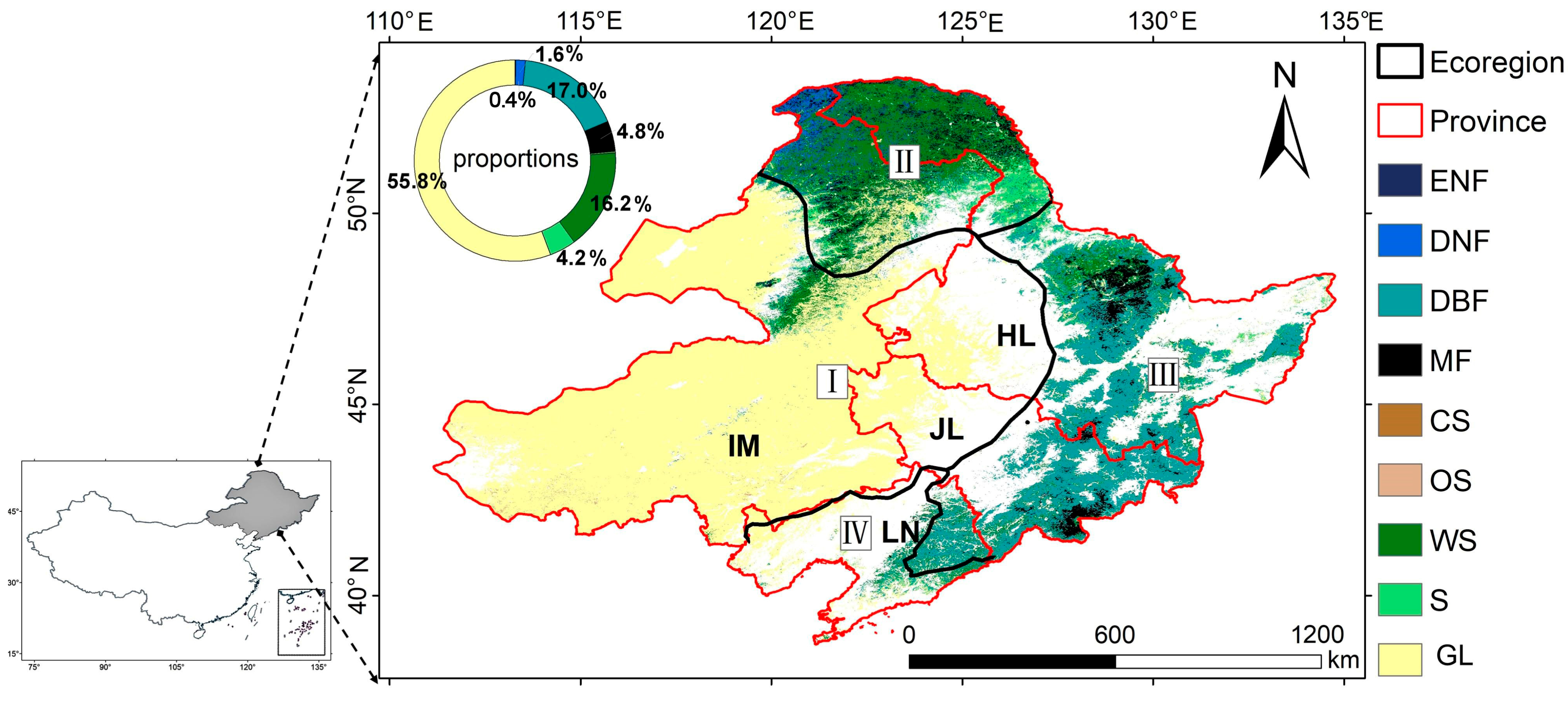
2.1. Study Area

The NEC encompasses the provinces of Heilongjiang, Jilin, Liaoning, and the eastern part of Inner Mongolia Autonomous Region, which includes Hulunbuir City, Xing’an League, Tongliao City, Chifeng City, and Xilin Gol League (Figure 1). The western region of NEC exhibits elevated terrain, with peaks reaching heights of up to 2600 m. NEC spans an expansive area of 1.4 million km² and encompasses China’s most extensive forested areas, particularly in the Greater and Lesser Khingan Mountains. The climate of the region is characterized by cold winters and cool summers, supporting a diverse range of vegetation. The NEC comprises four ecoregions: (I) temperate grasslands; (II) cold–temperate deciduous–coniferous forests; (III) temperate coniferous–broad-leaved mixed forests; and (IV) warm–temperate deciduous broad-leaved forests [39]. Due to its diverse vegetation and pronounced seasonal variations, the NEC serves as an ideal locale for studying plant phenology, particularly in the context of global climate change [31,32].

2.2. Remotely Sensed Data

In this study, the land cover/use data with 500 m resolution from yearly global MODIS product (MCD12Q1.061 https://lpdaac.usgs.gov/products/mcd12q1v061/, accessed on 15 March 2024) were applied to extract vegetation area (including forests and grasslands); the time series of NDVI data from the MODIS VI product (MOD13A1.061 https://lpdaac.usgs.gov/products/mod13a1v061/, accessed on 15 March 2024) with 500 m spatial and 16-day temporal resolution was applied to calculate kNDVI. These datasets can be obtained from NASA Land Processes Distributed Active Archive Center at the United States Geological Survey (USGS) Earth Resources Observation and Science Center (https://lpdaac.usgs.gov/, accessed on 15 March 2024). Because we focus on the phenology of vegetation, including forests and grassland, the nine vegetation types based on the International Geosphere-Biosphere Program (IGBP) [40] classification scheme were selected, including evergreen needleleaf forests (ENFs), deciduous needleleaf forests (DNFs), deciduous broadleaf forests (DBFs), mixed forests (MFs), closed shrublands (CS), open shrublands (OS), woody savannas (WS), savannas (S), and grasslands (GLs). The most abundant vegetation types were GLs (55.8%), DBFs (17.0%), and WS (16.2%).

Since temperature, precipitation, and drought events significantly impact plant phenology [22,38], a total of five climate factors were selected for analysis in this study: temperature (TEM), precipitation (PRE), potential evapotranspiration (PET) from 1 km monthly dataset for China provided by the Peng’s studies [41,42,43]; Palmer drought severity index (PDSI), and vapor pressure deficit (VPD) from TerraClimate global 4 km monthly climate dataset provided by the University of Idaho [44]. To ensure spatial alignment with MODIS-based phenological metrics (500 m), all climate datasets were resampled to 500 m using bilinear interpolation. Initial comparisons indicated that retaining the original 4 km resolution led to mismatches and reduced model performance in pixel-level analysis, supporting the decision to adopt a unified 500 m resolution for all variables. The climate variables used in this study are listed in

Table 1. The details of the climate factors selected in this study.

Name	Description	Units	Spatial Resolution
TEM	Temperature	°C	1 km
PRE	Precipitation	mm	1 km
PET	Potential evapotranspiration	mm	1 km
VPD	Vapor pressure deficit	kPa	4 km
PDSI	Palmer drought severity index	*	4 km

Note: The “*” notation represents “no units”.

. Their average values during the growing season (April to October) are illustrated in Figure 2. These monthly datasets were further seasonally aggregated for subsequent analysis. In addition, elevation data for the NEC were obtained from the CGIAR-CSI SRTM Version 4 dataset, which offers a spatial resolution of 90 m and has been post-processed to fill voids and improve accuracy. The DEM data were resampled to 500 m to match LSP indicators using bilinear interpolation and were categorized into 50 m intervals to analyze phenological changes across elevation gradients.

2.3. Ground-Based Phenological Observation Data

Ground-based phenological observation (GBPO) data were obtained from the National Earth System Science Data Center, National Science & Technology Infrastructure of China (http://www.geodata.cn, accessed on 15 March 2023), covering seven cities in Northeast China (NEC) with varying latitudes, longitudes, and elevations (

Table 2. Ground-based phenological observation data.

Year	City	Province	Latitude	Longitude	SOS	EOS	LOS	Vegetation Types
1974–1996	HH	HL	50.25°N	127.50°E	140	269	130	woody
1966–1996	JMS	HL	46.81°N	130.37°E	129	283	154	woody
1963–2012	HRB	HL	45.77°N	126.64°E	124	275	137	woody
1964–1996	MDJ	HL	44.58°N	129.62°E	125	261	138	woody
2014	HHHT	IM East	43.93°N	116.05°E	100	289	192	herbaceous
1986–2012	CC	JL	43.82°N	125.32°E	121	267	147	woody
1964–2012	SY	LN	41.81°N	123.43°E	116	261	146	woody

Note: HL—Heilongjiang, JL—Jilin, LN—Liaoning, IM East—Inner Mongolia East for province; HH—Heihe, JMS—Jiamusi, HRB—Harbin, MDJ—Mudanjiang, HHHT—Hohhot, CC—Changchun, and SY—Shenyang city.

). Although the number of observation sites is limited, each city contains long-term phenological records across multiple years (e.g., 1963–2012), reflecting average phenological trends rather than a single-year snapshot. The observations include phenological indicators (SOS and EOS) of dominant vegetation species in each city. While some records represent mixed vegetation types and lack consistent species-level classification, site-specific knowledge allows for general classification into woody (e.g., forest, shrubs) and herbaceous (e.g., grassland) categories. This binary grouping was adopted to match the remote sensing–derived land cover classification during LSP threshold calibration.

Although differences in scale and methods exist between ground-based and large-scale remote sensing observations [45], GBPO data remain the most reliable reference for validating phenological metrics. Therefore, this study calculated the multi-year average SOS and EOS values per site as reference points for remote sensing-based LSP extraction.

2.4. Methodology

Figure 3 shows the flowchart of this study. This study consists of three aims: (1) to generate high-quality 4-d LSP indicators and investigate the spatial patterns; (2) to analyze the phenology trends in different vegetation cover types; (3) to explore the response of LSP to climate factors in different seasons.

2.4.1. The Extraction of Phenology Indicators Based on 4-Day kNDVI Sequence

Since the kernel NDVI (kNDVI) demonstrates better performance compared to NDVI with nonlinear and saturation effects [16], the kNDVI was calculated using Equation (1) for phenology indicators extraction.

$$\mathrm{k}\mathrm{N}\mathrm{D}\mathrm{V}\mathrm{I}=\mathrm{t}\mathrm{a}\mathrm{n}\mathrm{h}{\left(\mathrm{N}\mathrm{D}\mathrm{V}\mathrm{I}\right)}^2$$

(1)

To address noise and increase temporal resolution from 16-day to 4-day, we applied linear interpolation and Savitzky–Golay (S-G) filtering to the kNDVI sequence, as shown in Figure 4a,b. We inserted 4-day intervals between the original 16-day kNDVI data points and used linear interpolation to fill these gaps, followed by S-G smoothing [46] for noise reduction and clearer seasonal patterns.

As shown in Figure 4c,d, to extract phenological dates, we adopted a dynamic threshold method based on the temporal curve of the smoothed 4-day kNDVI. In this method, SOS is defined as the date when kNDVI increases past a given percentage of the seasonal amplitude, and EOS is defined as the date when it declines below a corresponding threshold. The seasonal amplitude is calculated as the difference between the annual maximum and minimum kNDVI values. This method captures interannual variations in vegetation dynamics by adapting to each pixel’s own growth curve [10,18].

To determine the optimal dynamic threshold for extracting SOS and EOS, we tested a series of kNDVI thresholds ranging from 10% to 80% of the seasonal amplitude in 5% increments. For each threshold, we extracted the SOS and EOS dates from the smoothed 4-day kNDVI time series. These remotely-sensed dates were then compared against GBPO at corresponding locations and years. The mean absolute error (MAE) and root mean square error (RMSE) were calculated between the extracted and observed SOS/EOS dates for each threshold level. The thresholds yielding the lowest MAE and RMSE were considered optimal and applied in the full-scale extraction of phenological parameters [47,48].

To calibrate these thresholds and assess the accuracy of remote-sensing-based LSP extraction, GBPO data were used. While the classification of vegetation types in this study followed the IGBP scheme, the ground-based observation data lacked consistent species-level labels. Therefore, a simplified classification into woody and herbaceous types was adopted during LSP threshold calibration.

2.4.2. Trend Analysis of LSP Indicators

The Theil–Sen (TS) median slope trend analysis and the Mann–Kendall (M-K) test were used to evaluate long-term trends in LSP indicators (SOS, EOS, LOS) [23,49]. The TS slope reduces the influence of outliers, while the M-K test assesses the significance of trends at the 0.05 confidence level.

Based on the sign of the TS slope and the M-K Z value, phenological trends were classified into five types:

(1)

Significantly delayed or extended (slope > 0 and |Z| > 1.96);

(2)

Slightly delayed or extended (slope > 0 and |Z| ≤ 1.96);

(3)

Significantly advanced or shortened (slope < 0 and |Z| > 1.96);

(4)

Slightly advanced or shortened (slope < 0 and |Z| ≤ 1.96);

(5)

No significant change (slope = 0).

2.4.3. Response of LSP to Climate Factors

• Evaluation of the importance of seasonal climate variables

This study employed the importance scores from the random forest algorithm, a machine learning method that can be used to evaluate variable importance by measuring the increase in prediction error after permuting each variable (i.e., the decrease in mean squared error (MSE) calculation) [50]. This approach allows for quantifying the impact of climate variables on SOS, EOS, and LOS across different seasons to examine the influence and lag effect of climate factors on plant phenology [34]. According to the China Meteorological Administration (https://www.cma.gov.cn/, accessed on 20 April 2023), the seasons were defined as spring (March–May), summer (June–August), autumn (September–November), and winter (December–February) in this study. All the climate variables were resampled to 500 m to match LSP indicators using bilinear interpolation. To avoid the impact of inconsistent units, all the climate variables and LSP indicators were standardized using z-score normalization [51].

• Correlation analysis

To analyze the relationship between climate factors and LSP, this study employs pixel-wise Spearman’s correlation analysis [52] for the phenological indicators (including SOS, EOS, and LOS) and climate factors (including TEM, PRE, PET, VPD, and PDSI) across the different seasons from 2001 to 2021. To ensure the focus on the key climate factors influencing LSP and consider the lag effect, the most critical season was determined by selecting the season with the highest importance score from the random forest analysis for each climate variable. This guarantees that each climate variable in the correlation study coincides with the season having the most significant impact on the phenological indicators.

3. Results

3.1. The Extraction of LSP Indicators Using Optimal Dynamic Thresholds

As described in Section 2.4.1, this study evaluated the accuracy of different threshold levels by comparing the remotely sensed SOS and EOS dates with GBPO and calculated the MAE and RMSE for each threshold to identify the optimal one. Due to the significant difference between grasslands and non-grasslands, this study selected the optimal thresholds of LSP indicators (i.e., SOS and EOS) using GBPO data for grasslands and non-grasslands (including ENFs, DNFs, DBFs, MFs, CS, OS, WS, and S) regions separately. Based on the MAE and RMSE, the optimal thresholds were determined to be 10% for SOS and 15% for EOS in grasslands, and 50% for SOS and 45% for EOS in the non-grassland region (Figure 5). The thresholds were selected based on the lowest error values indicated by the different curves in Figure 5, ensuring that both the total and independent errors for SOS and EOS were considered. Then, the EOS and SOS were extracted using the optimal thresholds based on a 4-day kNDVI sequence for the entire NEC [47,48].

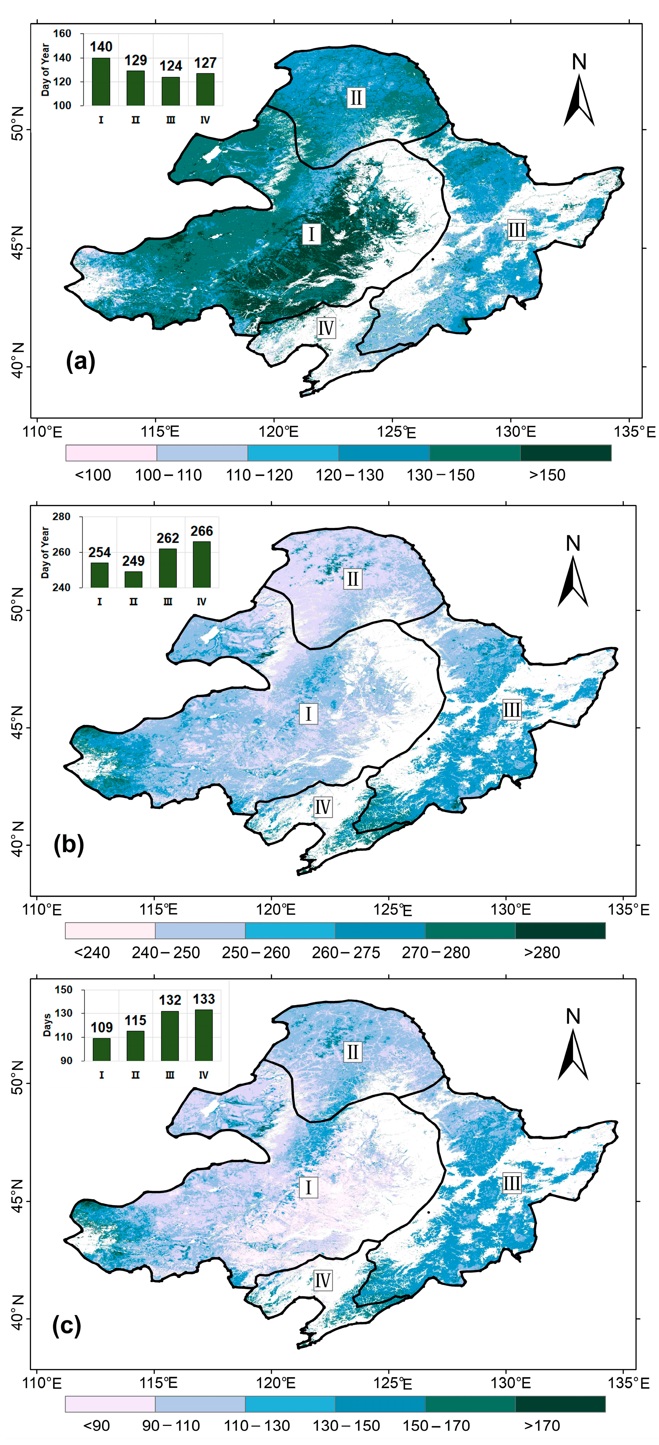
3.2. Spatiotemporal Trend of the LSP Indicators in the NEC

Figure 6a–c depicts the spatial distribution of extracted average phenological indicators from 2001 to 2021. In general, the NEC region exhibits distinct spatial heterogeneity, which is predominantly associated with vegetation types and ecoregions. In the NEC, SOS (Figure 6a) initiates later in grasslands than in forests, with temperate grasslands (ecoregion I) exhibiting the latest SOS (~140^th day), particularly in the eastern areas, showing a clear west-to-east gradient. In contrast, forests in ecoregions III and IV generally have earlier SOS (~125^th day) and smaller spatial variation. For EOS (Figure 6b), cold–temperate deciduous–coniferous forests (ecoregion II) exhibit the earliest EOS (~249^th day), while ecoregions III and IV show relatively later EOS (~260^th day). The EOS in ecoregion I displays an east–west variation, opposite to that of SOS, suggesting climatic control. LOS reflects the joint effects of SOS and EOS (Figure 6c). Ecoregions III and IV exhibit the longest growing seasons (132–133 days), while ecoregion I has the shortest LOS (~109 days), and ecoregion II falls in between (~115 days). This variation highlights the vegetation-type-dependent growing season duration in the NEC.

Figure 7 illustrates phenological differences across vegetation types. Forests (ENFs, DNFs, DBFs, and MFs) show the earliest SOS (~125^th day) and latest EOS (~260^th day), resulting in the longest LOS (~130 days) compared to other vegetation types (i.e., shrublands, savannas, and grassland), except DNFs. DNFs exhibit a slightly earlier EOS (~250^th day), leading to a relatively shorter LOS (~120 days). Shrubs (CS and OS) display the latest SOS (~150^th day) and the shortest LOS (~96 days). Savannas (S and WS) and grasslands (GLs) have intermediate values, with WS exhibiting slightly earlier SOS (~130^th day) and longer LOS (~120 days) than S, likely due to woody cover. Despite similar EOS timing (~250^th day) across most vegetation types, the marked variation in SOS primarily determines the difference in LOS.

Combining the results of Sen’s slope and M-K significance tests, as shown in Figure 8a, we found that for SOS, more than half of the region of NEC exhibited an advancing trend (54%), with 24% showing significant advancement, 34% showing no significant change, and only 12% of the area showing a delaying trend, mainly located in the northwest of the temperate grasslands (ecoregion I). Regarding the EOS shown in Figure 8b, over half of the area showed no significant change (51%), with 41% of the area exhibiting delays and 9% of the area exhibiting advances. The advanced area was mainly distributed in the northern parts of the cold–temperate deciduous–coniferous forests (ecoregion II), while other parts of this ecoregion mostly showed no significant change. As shown in Figure 8c, due to the advance and delay characteristics exhibited by SOS and EOS, respectively, most areas showed an extended trend (65%) for LOS (with 34% and 31% showing significant and slightly extending, respectively) and only 13% showed a shortening trend (with about 1% of the area having significant shortened LOS), mainly located in the northern regions of ecoregions I and II. The characteristics observed in different ecoregions may be related to their complex vegetation types and geographical locations.

The overall trend of the three phenological indicators for different natural vegetation types is very similar (Figure 9a–c). Notably, SOS shows a significant advancing trend, with the highest proportion of advancing SOS found in savannas (63%) and ENFs (62%), with the significant advancement accounting for 36% and 35%, respectively. The largest proportion of delayed SOS is observed in GLs (20%), while the largest proportion of phenologically stable area is observed in MFs (55% of the area shows no significant change). Most vegetation types show no significant change in EOS (especially Savannas), with the unchanged areas exceeding 40% (except for GLs). The primary trend for the length of season (LOS) is an extension, with the largest percentage of extended pixels observed in DBFs (83%), followed by S and ENFs (both at 73%). DBFs have the lowest percentage of shortened LOS, at a mere 2%, whereas GLs have the highest percentage, at 19%.

Figure 10 reveals that the most natural vegetation types show a significant advancement in SOS (about 0.2 days/year), a delay in EOS (about 0.1 days/year), and an extension in LOS (about 0.35 days/year), while shrubs (i.e., CS and OS) have the opposite trend. Coniferous forests (ENFs and DNFs) are a special case: the advancements in SOS are relatively small (less than 0.1 days/year); the EOS of coniferous forests also demonstrates an advancement rather than a delay, with the advancement in ENFs being more significant than that in DNFs. Owing to the advanced EOS, ENFs exhibit a shortening in LOS, while DNFs have the least tendency for LOS extension.

3.3. Response of LSP to Climate Factors

3.3.1. Gradient Relationship Between Elevation and LSP

Since the distribution of precipitation and temperature is closely related to elevation, investigating how LSP changes with elevation can help understand the response of LSP to climate factors [53,54,55]. Since the elevation of different vegetation types in the NEC varies, this study analyzed the gradient relationship between LSP and elevation for forests (including ENFs, DNFs, DBFs, and MFs), shrublands (including CS and OS), savannas (including S and WS), and grasslands separately. Elevation was categorized into 50 m intervals and shown with the mean and standard deviation for each class. According to Figure 11a,c,d, as the elevation increases 100 m, the SOS of forests, savannas, and grasslands delay by 1.2, 1.9, and 0.8 days (r = 0.84, 0.91, 0.40), respectively; the EOS of forests, savannas, and grasslands advance by 0.1, 0.2, and 0.2 days (r = −0.16, −0.39, −0.53), respectively; and the LOS of forests, savannas, and grasslands shortens by 0.1, 2.1, and 1.1 days (r = −0.72, −0.92, −0.51), respectively. On the other hand, the shrublands has the opposite trend (Figure 11b): as the elevation increases 100 m, the SOS advances by 0.8 days (r = −0.59), the EOS delays by 0.7 days (r = 0.61), and the LOS extends by 1.5 days, respectively (r = 0.58).

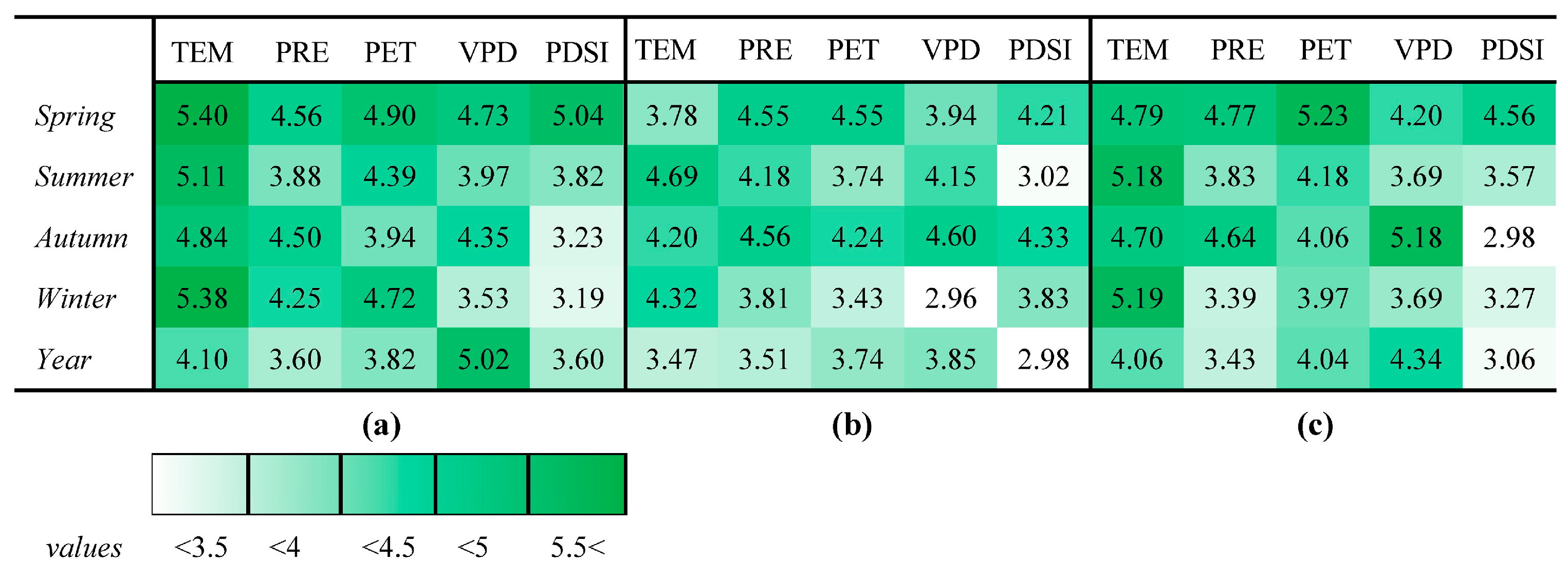
3.3.2. Evaluation of the Importance of Seasonal Climate Variables

The importance scores shown in Figure 12 were derived using the random forest regression models based on the mean decrease in the mean squared error (MSE). For each phenological indicator (SOS, EOS, and LOS), a separate model was built using seasonal climate variables as predictors. The importance scores were calculated using a random forest algorithm between the LSP indices and climate variables (TEM, PRE, PET, VPD, and PDSI) across different seasons. For SOS (see Figure 12a), the most important climate factor in all four seasons is TEM, whereas VPD exhibits stronger importance throughout the year. As for EOS (Figure 12b), PRE and PET in spring, TEM in summer, PDSI in autumn, and the annual average VPD are the most crucial. Regarding LOS (Figure 12c), PRE, PET, and PDSI in spring; TEM in summer and winter; and VPD in autumn are the most significant. It can be observed that the climate variables in different seasons have various impacts on LSP in NEC. Therefore, for different phenological indicators, the most influential seasons for each climate variable are finally selected and presented in

Table 3. Climate variables and their most influential seasons for different phenological indicators.

Variables	SOS	EOS	LOS
TEM	Spring	Summer	Summer
PRE	Spring	Autumn	Spring
PET	Spring	Spring	Spring
VPD	Year	Autumn	Autumn
PDSI	Spring	Autumn	Spring

Note: TEM—temperature, PRE—precipitation, PET—potential evapotranspiration, VPD—vapor pressure deficit, and PDSI—Palmer drought severity index.

. The climatic factors in their most influential seasons selected by the RF model were applied for the subsequent correlation analysis with phenological indicators.

3.3.3. Correlation Analysis

Among the various climatic factors influencing SOS, TEM (Figure 13(a-1)) and PDSI (Figure 13(e-1)) have the largest significant areas (25% and 24%, respectively). SOS is mostly negatively correlated with TEM and PDSI, but TEM shows a positive correlation with SOS in temperate grasslands (ecoregion I); PDSI has a positive correlation with SOS in the southeastern part of the NEC and a negative correlation in ecoregion I. PRE is widely negatively correlated with SOS in ecoregion I (Figure 13(b-1)), while it shows a positive correlation in other regions. The positive correlations between PET (Figure 13(c-1)) and VPD (Figure 13(d-1)) with SOS are also noteworthy, accounting for 84% and 81% of the areas, respectively, mainly distributed in the southwestern and central–northern parts of the NEC.

For EOS, PRE has the most significant impact (Figure 13(b-2)), with a total significant correlation area of 27%, of which 87% is positively correlated, except for cold–temperate deciduous–coniferous forests (ecoregion II). TEM also shows a notable positive correlation with EOS (Figure 13(a-2)), with 75% of the area positively correlated and 89% of the significant correlations being positive. PDSI is also mainly positively correlated with EOS (Figure 13(e-2)), with up to 92% of the significant correlation area being positively correlated. In contrast, VPD has the strongest negative correlation with EOS (Figure 13(d-2)), accounting for 81% of the pixels and 96% of the significant correlation pixels, widely distributed in all regions except the southern part of cold–temperate deciduous–coniferous forests (ecoregion II).

Unlike SOS and EOS, the correlations between LOS and TEM (Figure 13(a-3)) or PRE (Figure 13(b-3)) are not the most prominent, but their positive correlations with LOS can still be observed. PDSI (Figure 13(e-3)) and VPD (Figure 13(d-3)) have the largest significantly correlated areas with LOS, at 22% and 21%, respectively. VPD is mainly negatively correlated with LOS (81% negatively correlated and 96% significantly negatively correlated), mainly distributed in the central and eastern parts of the NEC. PDSI is mainly positively correlated with LOS (77% positively correlated and 94% significantly positively correlated), showing a distinct north–south distribution pattern, with positive correlations mainly in the north and negative correlations mainly in the south. The geographical distribution of the correlation between PET and LOS (Figure 13(c-3)) is opposite to that between PET and SOS (Figure 13(c-1)).

4. Discussion

4.1. Spatial Pattern of LSP in the NEC

This study reveals that the LSP in the NEC demonstrates significant spatial heterogeneity, with clear differences among vegetation types and ecoregions. Forests exhibit an earlier SOS (117–129^th day), a later EOS (251–271^st day), and a longer LOS (122–142 days), while shrubs and grasslands show delayed SOS and shorter LOS.

The phenological indicators for forests in NEC fall within the ranges reported in previous studies [30,56], yet show reduced variability (SOS: 117–129^th day; EOS: 251–271^st day; LOS: 122–142 days), suggesting that the dynamic threshold method based on the kNDVI used here captures more stable phenological characteristics. For example, Hou [30] and Yu and Zhuang [56] reported SOS of forests in NEC ranging from the 110^th to 140^th day and 100^th to 150^th day, respectively, an EOS ranging from the 260^th to 290^th day, and the LOS ranging from 120–160 days and 140–180 days, respectively. Compared to these studies, this work reflects not only narrower ranges but also more consistent spatial patterns across forest types.

Ecoregion-level comparisons also support these patterns. Ecoregion II (cold–temperate deciduous–coniferous forests) exhibits the earliest EOS (252^nd day). Ecoregion I (temperate grasslands) shows a significant east–west variation across all three LSP indicators, with the latest SOS (140^th day), early EOS (255^th day), and shortest LOS (116 days). These differences reflect vegetation-specific phenological responses, possibly driven by regional climatic and topographic factors. For instance, the delayed SOS of grasslands in ecoregion I may be associated with lower spring precipitation (Figure 2c), aligning with prior findings that grassland phenology is sensitive to moisture availability [57].

Elevation further modulates phenological patterns across vegetation types. According to Hopkins’ Bioclimatic Law [54], leaf-out (i.e., SOS) is progressively delayed and leaf senescence (i.e., EOS) is advanced with increasing elevation. For every 100 m increase in elevation, this study found that the change in SOS in forests, savannas, and grasslands is consistent with Hopkins’ Bioclimatic Law. Nevertheless, the delay for SOS in NEC forests (1.2 days) is much shorter compared to the Alps (2.4–3.2 days) but similar to the Qinghai–Tibet Plateau (1.1 days) [58,59].

4.2. Trend of LSP in the NEC

This study revealed that the SOS in the NEC advanced at a rate of 0.23 days per year, the EOS delay rate was 0.12 days per year, and the LOS extended at a rate of 0.38 days per year. These trends were consistent with existing research findings [32,60,61,62] but were not found in the northern parts of temperate grasslands (ecoregion I) and cold–temperate deciduous–coniferous forests (ecoregion II), as shown in Figure 8. Therefore, this study further investigated the LSP trend changes in different natural vegetation types (Figure 10). Except for coniferous forests (including ENFs and DNFs) and shrubs (including CS and OS), all vegetation types showed a significant advancement in SOS (Sen’s slope < −0.1), a delay in EOS (Sen’s slope > 0), and an extension in LOS (Sen’s slope > 0.1) (Figure 10). The trend of slight variation in SOS and a significant advance in EOS was also found in coniferous forests in another East Asian LSP study [20]. The different phenological trends exhibited by coniferous forests are noteworthy and worthy of further exploration. Coniferous forests are typically found in high-latitude regions where climate change is more pronounced than in other regions. Their thick bark helps resist cold and retain moisture, reducing sensitivity to warmth, leading to different LSP trends compared to other forest types [63,64]. Furthermore, ENFs require an earlier EOS for dormancy to prevent leaf cell freezing and dehydration, while DNFs shed leaves to reduce water and nutrient loss, resulting in a later EOS [63,64].

4.3. Response of LSP to Climate Factors

Regarding the response of LSP to climate factors, TEM and PRE are the most critical climate factors for spring and autumn phenology, respectively, which is consistent with previous studies [20,21,22]. But TEM exerts the greatest influence on annual phenology (Figure 12), which may be attributed to the more frequent occurrence of extreme temperatures than extreme precipitation in NEC and the fact that extreme precipitation can lead to changes in temperature [65]. The correlation results show that SOS is negatively correlated with TEM (Figure 13(a-1)), which is consistent with Feng [23] and Tao [22]. Although both PDSI and PRE are related to water, PDSI has a greater impact on spring phenology (SOS), while PRE has a greater impact on autumn phenology (EOS). It is also observed that spring PET has legacy effects on autumn phenology (see Table 3). Liu [66] also emphasized that early-season hydroclimatic conditions can have lasting impacts on vegetation phenology. PDSI is related to both precipitation and evapotranspiration, primarily reflecting long-term changes in soil moisture (soil moisture promotes an earlier SOS), while PRE generally represents short-term external changes (precipitation sustains plant growth, leading to a delayed EOS) [67]. It is also noteworthy that PRE is negatively correlated with EOS only in cold–temperate deciduous–coniferous forests (ecoregion II) (Figure 13(b-2)). This may be because the precipitation cannot be quickly utilized in high-latitude forests, as increasing the evaporation cooling effect would result in local cooling and advancing the EOS [68]. In addition, although rising TEM usually advances SOS, increasing PRE usually delays SOS; this is opposite in temperate grasslands (ecoregion I), which is due to grasslands’ greater sensitivity to precipitation rather than temperature. Ren [69] attributed this phenomenon to the fact that increased rainfall quickly translates into usable water, advancing the SOS, while rising temperatures may lead to drought, subsequently delaying the SOS.

4.4. Limitations and Future Work

This study holds significant implications for analyzing the relationship between plant phenological patterns and climate change in NEC from 2001 to 2021, but it still faces several challenges. First, MODIS only provides data at relatively coarse resolutions of 250 m, 500 m and 1 km [12] (this study chose a 500 m resolution to match the land cover/use data), resulting in the loss of detailed phenological information and the variations in the definitions of phenological indicators obtained from remote sensing and GBPO data [17]. However, validating the remote sensing-derived LSP indicators using in situ field observations is crucial [70]. The gap will be gradually bridged by advances in new satellites with fine-scale spatial and high temporal resolution (such as PlanetScope); unmanned aerial vehicles; and a large number of GBPO networks, including the Pan-European Phenological Network (PEPN), the American Phenological Network National Phenological Network (NPN), and phenological photos from Phenocam [17,70,71,72,73,74]. However, few of these GBPO networks are distributed in Asia, especially in China [75]. The future study will concentrate on conducting high-resolution, fine-scale phenological research by utilizing multi-platform remote sensing data. The aim is to address the limitations of current phenological studies, such as the discrepancies in phenological observations due to the insufficient high spatial and temporal remote sensing data. Second, it should be noted that the phenological DOY values derived from MODIS are based on nominal composite dates and may not represent precise acquisition times [76]. Therefore, this study focuses on the spatial and temporal patterns and gradients of phenology rather than exact day comparisons. While qualitative comparisons of phenological indices across various vegetation types are not affected by temporal uncertainty in composite MODIS data, it remains essential to further evaluate and mitigate the impact of this temporal uncertainty when extracting the absolute phenological Day of Year (DOY) values for each vegetation type. Third, the dynamic threshold method provides optimal thresholds that vary with spatial heterogeneity, influenced by changes in latitude, longitude, and vegetation types [77]. However, this study only set thresholds for grasslands and non-grasslands because validation is limited when setting more thresholds due to limited GBPO records. In the future, the thresholds used to extract the LSP indicators could be optimized according to different forest types if the GBPO records or other phenological observations are sufficient. Hence, it is imperative for future studies to prioritize the examination of the retrieval of detailed phenological indicators by utilizing a combination of multi-platform remote sensing data and optimized thresholds based on forest types or even pixels. Additionally, it is crucial to explore the delayed impact of climatic factors and hydrological factors on phenology [78].

5. Conclusions

This study generated high-quality 4-day LSP indicators and explored the LSP patterns, trends across ecoregions and vegetation types, and responses to seasonal climate factors in NEC from 2001 to 2021. Marked spatial heterogeneity was observed, with forests showing the earliest start of season (SOS) and longest length of season (LOS), while shrublands exhibited the latest SOS and shortest LOS. Grasslands displayed pronounced east–west gradients in SOS and EOS. Over the past two decades, SOS advanced by 0.23 days/year, EOS delayed by 0.12 days/year, and LOS extended by 0.38 days/year. Coniferous forests show opposite trends due to their cold-resistant traits, especially for evergreen needle-leaved forests (ENFs), which require an earlier EOS for dormancy to prevent leaf cell freezing and dehydration. In the NEC, temperature has the greatest influence on LSP; rising temperature will lead to an advancing SOS. However, for temperate grasslands (ecoregion I), which have greater sensitivity to precipitation rather than temperature, increasing rainfall would advance the SOS, but rising temperatures may lead to drought, subsequently delaying the SOS. Drought (e.g., reflected by PDSI) significantly influenced spring phenology, while increased precipitation was associated with earlier EOS in regions where moisture could not be effectively utilized. By integrating high-resolution phenology and diverse seasonal climate factors, this study offers new insights into vegetation-specific and ecoregion-based phenological dynamics under climate change, providing a foundation for future ecological forecasting and adaptive management.

References

1. Lieth, H. Phenology in Productivity Studies. In Analysis of Temperate Forest Ecosystems; Reichle, D.E., Ed.; Springer: Berlin/Heidelberg, Germany, 1973; pp. 29–46. [Google Scholar] [CrossRef]
2. Roetzer, T.; Wittenzeller, M.; Haeckel, H.; Nekovar, J. Phenology in Central Europe—Differences and Trends of Spring Phenophases in Urban and Rural Areas. Int. J. Biometeorol. 2000, 44, 60–66. [Google Scholar] [CrossRef] [PubMed]
3. Richardson, A.D.; Keenan, T.F.; Migliavacca, M.; Ryu, Y.; Sonnentag, O.; Toomey, M. Climate Change, Phenology, and Phenological Control of Vegetation Feedbacks to the Climate System. Agric. For. Meteorol. 2013, 169, 156–173. [Google Scholar] [CrossRef]
4. de Beurs, K.M.; Henebry, G.M. Land Surface Phenology, Climatic Variation, and Institutional Change: Analyzing Agricultural Land Cover Change in Kazakhstan. Remote Sens. Environ. 2004, 89, 497–509. [Google Scholar] [CrossRef]
5. Xu, X.; Zhou, G.; Du, H.; Mao, F.; Xu, L.; Li, X.; Liu, L. Combined MODIS Land Surface Temperature and Greenness Data for Modeling Vegetation Phenology, Physiology, and Gross Primary Production in Terrestrial Ecosystems. Sci. Total Environ. 2020, 726, 137948. [Google Scholar] [CrossRef]
6. Ma, X.; Zhu, X.; Xie, Q.; Jin, J.; Zhou, Y.; Luo, Y.; Liu, Y.; Tian, J.; Zhao, Y. Monitoring Nature’s Calendar from Space: Emerging Topics in Land Surface Phenology and Associated Opportunities for Science Applications. Glob. Change Biol. 2022, 28, 7186–7204. [Google Scholar] [CrossRef]
7. Post, E.; Stenseth, N.C. Climatic Variability, Plant Phenology, and Northern Ungulates. Ecology 1999, 80, 1322–1339. [Google Scholar] [CrossRef]
8. Katal, N.; Rzanny, M.; Mäder, P.; Wäldchen, J. Deep Learning in Plant Phenological Research: A Systematic Literature Review. Front. Plant Sci. 2022, 13, 805738. [Google Scholar] [CrossRef]
9. Zhong, R.; Yan, K.; Gao, S.; Yang, K.; Zhao, S.; Ma, X.; Zhu, P.; Fan, L.; Yin, G. Response of Grassland Growing Season Length to Extreme Climatic Events on the Qinghai-Tibetan Plateau. Sci. Total Environ. 2024, 909, 168488. [Google Scholar] [CrossRef]
10. Jönsson, P.; Eklundh, L. TIMESAT—A Program for Analyzing Time-Series of Satellite Sensor Data. Comput. Geosci. 2004, 30, 833–845. [Google Scholar] [CrossRef]
11. Chang, Q.; Xiao, X.; Jiao, W.; Wu, X.; Doughty, R.; Wang, J.; Du, L.; Zou, Z.; Qin, Y. Assessing Consistency of Spring Phenology of Snow-Covered Forests as Estimated by Vegetation Indices, Gross Primary Production, and Solar-Induced Chlorophyll Fluorescence. Agric. For. Meteorol. 2019, 275, 305–316. [Google Scholar] [CrossRef]
12. Huete, A.; Didan, K.; Miura, T.; Rodriguez, E.P.; Gao, X.; Ferreira, L.G. Overview of the Radiometric and Biophysical Performance of the MODIS Vegetation Indices. Remote Sens. Environ. 2002, 83, 195–213. [Google Scholar] [CrossRef]
13. Myneni, R.B.; Hoffman, S.; Knyazikhin, Y.; Privette, J.L.; Glassy, J.; Tian, Y.; Wang, Y.; Song, X.; Zhang, Y.; Smith, G.R.; et al. Global Products of Vegetation Leaf Area and Fraction Absorbed PAR from Year One of MODIS Data. Remote Sens. Environ. 2002, 83, 214–231. [Google Scholar] [CrossRef]
14. Tucker, C.J. Red and Photographic Infrared Linear Combinations for Monitoring Vegetation. Remote Sens. Environ. 1979, 8, 127–150. [Google Scholar] [CrossRef]
15. Zhou, L.; Zhou, W.; Chen, J.; Xu, X.; Wang, Y.; Zhuang, J.; Chi, Y. Land Surface Phenology Detections from Multi-Source Remote Sensing Indices Capturing Canopy Photosynthesis Phenology across Major Land Cover Types in the Northern Hemisphere. Ecol. Indic. 2022, 135, 108579. [Google Scholar] [CrossRef]
16. Wang, Q.; Moreno-Martínez, Á.; Muñoz-Marí, J.; Campos-Taberner, M.; Camps-Valls, G. Estimation of Vegetation Traits with Kernel NDVI. ISPRS J. Photogramm. Remote Sens. 2023, 195, 408–417. [Google Scholar] [CrossRef]
17. Zeng, L.; Wardlow, B.D.; Xiang, D.; Hu, S.; Li, D. A Review of Vegetation Phenological Metrics Extraction Using Time-Series, Multispectral Satellite Data. Remote Sens. Environ. 2020, 237, 111511. [Google Scholar] [CrossRef]
18. Xia, C. Review of Advances in Vegetation Phenology Monitoring by Remote Sensing. Natl. Remote Sens. Bull. 2013, 17, 1–16. [Google Scholar] [CrossRef]
19. Puchi, P.F.; Castagneri, D.; Rossi, S.; Carrer, M. Wood Anatomical Traits in Black Spruce Reveal Latent Water Constraints on the Boreal Forest. Glob. Change Biol. 2020, 26, 1767–1777. [Google Scholar] [CrossRef]
20. Wang, J.; Meng, S.; Zhu, W.; Xu, Z. Phenological Changes and Their Influencing Factors under the Joint Action of Water and Temperature in Northeast Asia. Remote Sens. 2023, 15, 5298. [Google Scholar] [CrossRef]
21. Yang, Y.; Fan, F. Land Surface Phenology and Its Response to Climate Change in the Guangdong-Hong Kong-Macao Greater Bay Area during 2001–2020. Ecol. Indic. 2023, 154, 110728. [Google Scholar] [CrossRef]
22. Tao, Z.; Wang, H.; Liu, Y.; Xu, Y.; Dai, J. Phenological Response of Different Vegetation Types to Temperature and Precipitation Variations in Northern China during 1982–2012. Int. J. Remote Sens. 2017, 38, 3236–3252. [Google Scholar] [CrossRef]
23. Feng, Z.; Chen, J.; Huang, R.; Yang, Y.; You, H.; Han, X. Spatial and Temporal Variation in Alpine Vegetation Phenology and Its Response to Climatic and Topographic Factors on the Qinghai-Tibet Plateau. Sustainability 2022, 14, 12802. [Google Scholar] [CrossRef]
24. Fang, X.; Zhu, Q.; Chen, H.; Ma, Z.; Wang, W.; Song, X.; Zhao, P.; Peng, C. Analysis of Vegetation Dynamics and Climatic Variability Impacts on Greenness across Canada Using Remotely Sensed Data from 2000 to 2009. J. Appl. Remote Sens. 2014, 8, 083666. [Google Scholar] [CrossRef]
25. Gaertner, B.A.; Zegre, N.; Warner, T.; Fernandez, R.; He, Y.; Merriamb, E.R. Climate, Forest Growing Season, and Evapotranspiration Changes in the Central Appalachian Mountains, USA. Sci. Total Environ. 2019, 650, 1371–1381. [Google Scholar] [CrossRef]
26. Guo, S.; Bai, H.; Huang, X.; Meng, Q.; Zhao, T. Remote Sensing Phenology of Larix chinensis Forest in Response to Climate Change in Qinling Mountains. Chin. J. Ecol. 2019, 38, 1123–1132. Available online: https://www.cje.net.cn/CN/Y2019/V38/I4/1123 (accessed on 15 March 2024). (In Chinese).
27. Kovalskyy, V.; Henebry, G.M. Alternative Methods to Predict Actual Evapotranspiration Illustrate the Importance of Accounting for Phenology—Part 2: The Event Driven Phenology Model. Biogeosciences 2012, 9, 161–177. [Google Scholar] [CrossRef]
28. Huang, J.-G.; Zhang, Y.; Wang, M.; Yu, X.; Deslauriers, A.; Fonti, P.; Liang, E.; Makinen, H.; Oberhuber, W.; Rathgeber, C.B.K.; et al. A Critical Thermal Transition Driving Spring Phenology of Northern Hemisphere Conifers. Glob. Change Biol. 2023, 29, 1606–1617. [Google Scholar] [CrossRef]
29. Ren, S.; Li, Y.; Peichl, M. Diverse Effects of Climate at Different Times on Grassland Phenology in Mid-Latitude of the Northern Hemisphere. Ecol. Indic. 2020, 113, 106260. [Google Scholar] [CrossRef]
30. Hou, X.; Niu, Z.; Gao, S. Phenology of Forest Vegetation in Northeast of China in Ten Years Using Remote Sensing. Spectrosc. Spectr. Anal. 2014, 34, 515–519. [Google Scholar] [CrossRef]
31. Zhang, Y.; Li, L.; Wang, H.; Zhang, Y.; Wang, N.; Chen, J. Land Surface Phenology of Northeast China during 2000–2015: Temporal Changes and Relationships with Climate Changes. Environ. Monit. Assess. 2017, 189, 531. [Google Scholar] [CrossRef]
32. Yu, X.; Wang, Q.; Yan, H.; Wang, Y.; Wen, K.; Zhuang, D.; Wang, Q. Forest Phenology Dynamics and Its Responses to Meteorological Variations in Northeast China. Adv. Meteorol. 2014, 2014, 592106. [Google Scholar] [CrossRef]
33. Yuan, M.; Zhao, L.; Lin, A.; Wang, L.; Li, Q.; She, D.; Qu, S. Impacts of Preseason Drought on Vegetation Spring Phenology across the Northeast China Transect. Sci. Total Environ. 2020, 738, 140297. [Google Scholar] [CrossRef] [PubMed]
34. Wang, C.; Jiang, Q.; Deng, X.; Lv, K.; Zhang, Z. Spatio-Temporal Evolution, Future Trend and Phenology Regularity of Net Primary Productivity of Forests in Northeast China. Remote Sens. 2020, 12, 3670. [Google Scholar] [CrossRef]
35. Shen, X.; Liu, B.; Henderson, M.; Wang, L.; Jiang, M.; Lu, X. Vegetation Greening, Extended Growing Seasons, and Temperature Feedbacks in Warming Temperate Grasslands of China. J. Clim. 2022, 35, 5103–5117. [Google Scholar] [CrossRef]
36. Wu, R.; Zhang, H.; Zhao, J.; Yu, S.; Guo, X.; Hong, Y.; Deng, G.; Li, H. Promote the Advance of the Start of the Growing Season from Combined Effects of Climate Change and Wildfire. Ecol. Indic. 2021, 125, 107483. [Google Scholar] [CrossRef]
37. Meng, F.; Zhou, Y.; Cui, S.; Wang, Q.; Tsechoe, D.; Wang, S. Effects of Climate Changes on Plant Phenology at High-Latitude and Alpine Regions. J. Univ. Chin. Acad. Sci. 2017, 34, 498–507. Available online: http://journal.ucas.ac.cn/EN/10.7523/j.issn.2095-6134.2017.04.012 (accessed on 15 March 2024).
38. Wang, J.; Zhou, T.; Peng, P. Phenology Response to Climatic Dynamic across China’s Grasslands from 1985 to 2010. ISPRS Int. J. Geo-Inf. 2018, 7, 290. [Google Scholar] [CrossRef]
39. Su, Y.; Guo, Q.; Hu, T.; Guan, H.; Jin, S.; An, S.; Chen, X.; Guo, K.; Hao, Z.; Hu, Y.; et al. An Updated Vegetation Map of China (1:1000000). Sci. Bull. 2020, 65, 1125–1136. [Google Scholar] [CrossRef]
40. Friedl, M.; Sulla-Menashe, D. MODIS/Terra+Aqua Land Cover Type Yearly L3 Global 500m SIN Grid V061. NASA LP DAAC. 2022. Available online: https://lpdaac.usgs.gov/products/mcd12q1v061/ (accessed on 15 March 2024).
41. Peng, S. 1 km Monthly Potential Evapotranspiration Dataset for China (1901–2023). National Tibetan Plateau/Third Pole Environment Data Center. 2022. Available online: https://data.tpdc.ac.cn/en/data/8b11da09-1a40-4014-bd3d-2b86e6dccad4 (accessed on 15 March 2024).
42. Peng, S. 1-km Monthly Precipitation Dataset for China (1901–2023). National Tibetan Plateau/Third Pole Environment Data Center. 2020. Available online: https://data.tpdc.ac.cn/en/data/faae7605-a0f2-4d18-b28f-5cee413766a2 (accessed on 15 March 2024).
43. Peng, S. 1-km Monthly Mean Temperature Dataset for China (1901–2023). National Tibetan Plateau/Third Pole Environment Data Center. 2019. Available online: https://data.tpdc.ac.cn/en/data/71ab4677-b66c-4fd1-a004-b2a541c4d5bf/ (accessed on 15 March 2024).
44. Abatzoglou, J.T.; Dobrowski, S.Z.; Parks, S.A.; Hegewisch, K.C. TerraClimate, a High-Resolution Global Dataset of Monthly Climate and Climatic Water Balance from 1958–2015. Sci. Data 2018, 5, 170191. [Google Scholar] [CrossRef]
45. Berra, E.F.; Gaulton, R. Remote Sensing of Temperate and Boreal Forest Phenology: A Review of Progress, Challenges and Opportunities in the Intercomparison of In-Situ and Satellite Phenological Metrics. For. Ecol. Manag. 2021, 480, 118663. [Google Scholar] [CrossRef]
46. Savitzky, A.; Golay, M.J.E. Smoothing and Differentiation of Data by Simplified Least Squares Procedures. Anal. Chem. 1964, 36, 1627–1639. [Google Scholar] [CrossRef]
47. Li, J.; Tang, Z.; Deng, G.; Sang, G.; Wang, J. Remote Sensing Monitoring of Grassland Phenological Changes in the Qinghai-Tibetan Plateau During 2001–2020. Res. Soil Water Conserv. 2023, 30, 265–274. (In Chinese) [Google Scholar] [CrossRef]
48. Tian, Y. Multi-Scale Study on the Response of Vegetation Phenology to Climate Change in the Heilongjiang Basin. Ph.D. Thesis, University of Chinese Academy of Sciences (Northeast Institute of Geography and Agroecology, Chinese Academy of Sciences), Changchun, China, 2020. (In Chinese) [Google Scholar] [CrossRef]
49. Tian, Y.; Bai, X.; Wang, S.; Qin, L.; Li, Y. Spatial-Temporal Changes of Vegetation Cover in Guizhou Province, Southern China. Chin. Geogr. Sci. 2017, 27, 25–38. [Google Scholar] [CrossRef]
50. Genuer, R.; Poggi, J.; Tuleau-Malot, C. Variable Selection Using Random Forests. Pattern Recognit. Lett. 2010, 31, 2225–2236. [Google Scholar] [CrossRef]
51. Philipp, M.; Wegmann, M.; Kubert-Flock, C. Quantifying the Response of German Forests to Drought Events via Satellite Imagery. Remote Sens. 2021, 13, 1845. [Google Scholar] [CrossRef]
52. Sedgwick, P. Statistical Question: Spearman’s Rank Correlation Coefficient. BMJ-Br. Med. J. 2014, 349, g7327. [Google Scholar] [CrossRef]
53. Gao, M.; Wang, X.; Meng, F.; Liu, Q.; Li, X.; Zhang, Y.; Piao, S. Three-dimensional change in temperature sensitivity of northern vegetation phenology. Glob. Change Biol. 2020, 26, 5189–5201. [Google Scholar] [CrossRef]
54. Hopkins, A.D. The Bioclimatic Law. J. Wash. Acad. Sci. 1920, 10, 34–40. Available online: https://www.jstor.org/stable/24521154 (accessed on 15 March 2024).
55. Liu, X.; Zhu, X.; Zhu, W.; Pan, Y.; Zhang, C.; Zhang, D. Changes in Spring Phenology in the Three-Rivers Headwater Region from 1999 to 2013. Remote Sens. 2014, 6, 9130–9144. [Google Scholar] [CrossRef]
56. Yu, X.; Zhuang, D. Monitoring Forest Phenophases of Northeast China based on MODIS NDVI Data. Resour. Sci. 2006, 28, 111–117. Available online: https://www.resci.cn/CN/Y2006/V28/I4/111 (accessed on 15 March 2024). (In Chinese).
57. Wei, X.; Xu, M.; Zhao, H.; Liu, X.; Guo, Z.; Li, X.; Zha, T. Exploring Sensitivity of Phenology to Seasonal Climate Differences in Temperate Grasslands of China Based on Normalized Difference Vegetation Index. Land 2024, 13, 399. [Google Scholar] [CrossRef]
58. Pellerin, M.; Delestrade, A.; Mathieu, G.; Rigault, O.; Yoccoz, N.G. Spring tree phenology in the Alps: Effects of air temperature, altitude and local topography. Eur. J. For. Res. 2012, 131, 1957–1965. [Google Scholar] [CrossRef]
59. Shen, M.; Zhang, G.; Cong, N.; Wang, S.; Kong, W.; Piao, S. Increasing altitudinal gradient of spring vegetation phenology during the last decade on the Qinghai-Tibetan Plateau. Agric. For. Meteorol. 2014, 189, 71–80. [Google Scholar] [CrossRef]
60. Chang, S.; He, H.S.; Huang, F.; Krohn, J. Spring temperature and snow cover co-regulate variations of forest phenology in Changbai Mountains, Northeast China. Eur. J. For. Res. 2023, 143, 547–560. [Google Scholar] [CrossRef]
61. Zhang, Y.; Yin, P.; Li, X.; Niu, Q.; Wang, Y.; Cao, W.; Huang, J.; Chen, H.; Yao, X.; Yu, L.; et al. The divergent response of vegetation phenology to urbanization: A case study of Beijing city, China. Sci. Total Environ. 2022, 803, 150079. [Google Scholar] [CrossRef]
62. Zhao, J.; Wang, Y.; Zhang, Z.; Zhang, H.; Guo, X.; Yu, S.; Du, W.; Huang, F. The Variations of Land Surface Phenology in Northeast China and Its Responses to Climate Change from 1982 to 2013. Remote Sens. 2016, 8, 400. [Google Scholar] [CrossRef]
63. Sakai, A.; Larcher, W. Frost Survival of Plants: Responses and Adaptation to Freezing Stress; Springer Science and Business Media: Berlin/Heidelberg, Germany, 2012; Available online: https://link.springer.com/book/10.1007/978-3-642-71745-1 (accessed on 15 March 2024).
64. Tranquillini, W. Physiological Ecology of the Alpine Timberline: Tree Existence at High Altitudes with Special Reference to the European Alps; Springer Science & Business Media: Berlin/Heidelberg, Germany, 2012; Available online: https://link.springer.com/book/10.1007/978-3-642-67107-4 (accessed on 15 March 2024).
65. Zhai, P.; Pan, X. Change in Extreme Temperature and Precipitation over Northern China During the Second Half of the 20th Century. Acta Geogr. Sin. 2003, 58, 1–10. [Google Scholar] [CrossRef]
66. Liu, Y.Y.; van Dijk, A.I.J.M.; de Jeu, R.A.M.; Canadell, J.G.; McCabe, M.F.; Evans, J.P.; Wang, G. Recent reversal in loss of global terrestrial biomass. Nat. Clim. Chang. 2015, 5, 470–474. [Google Scholar] [CrossRef]
67. Cook, B.; Smerdon, J.; Seager, R.; Coats, S. Global warming and 21st century drying. Clim. Dynam. 2014, 43, 2607–2627. [Google Scholar] [CrossRef]
68. Chen, X.; Zhang, Y. Impacts of climate, phenology, elevation and their interactions on the net primary productivity of vegetation in Yunnan, China under global warming. Ecol. Indic. 2023, 154, 110533. [Google Scholar] [CrossRef]
69. Ren, S.; Peichl, M. Enhanced spatiotemporal heterogeneity and the climatic and biotic controls of autumn phenology in northern grasslands. Sci. Total Environ. 2021, 788, 147806. [Google Scholar] [CrossRef] [PubMed]
70. Dronova, I.; Taddeo, S. Remote sensing of phenology: Towards the comprehensive indicators of plant community dynamics from species to regional scales. J. Ecol. 2022, 110, 1460–1484. [Google Scholar] [CrossRef]
71. Mayer, A. Phenology and Citizen Science: Volunteers have documented seasonal events for more than a century, and scientific studies are benefiting from the data. Bioscience 2010, 60, 172–175. [Google Scholar] [CrossRef]
72. Richardson, A.D.; Hufkens, K.; Milliman, T.; Frolking, S. Intercomparison of phenological transition dates derived from the PhenoCam Dataset V1.0 and MODIS satellite remote sensing. Sci. Rep. 2018, 8, 5679. [Google Scholar] [CrossRef]
73. Templ, B.; Koch, E.; Bolmgren, K.; Ungersböck, M.; Paul, A.; Scheifinger, H.; Rutishauser, T.; Busto, M.; Chmielewski, F.-M.; Hájková, L.; et al. Pan European Phenological database (PEP725): A single point of access for European data. Int. J. Biometeorol. 2018, 62, 1109–1113. [Google Scholar] [CrossRef]
74. Wheeler, K.I.; Dietze, M.C. Improving the monitoring of deciduous broadleaf phenology using the Geostationary Operational Environmental Satellite (GOES) 16 and 17. Biogeosciences 2021, 18, 1971–1985. [Google Scholar] [CrossRef]
75. Wei, B.; Wei, J.; Jia, X.; Ye, Z.; Yu, S.; Yin, S. Spatiotemporal Patterns of Land Surface Phenology from 2001 to 2021 in the Agricultural Pastoral Ecotone of Northern China. Sustainability 2023, 15, 5830. [Google Scholar] [CrossRef]
76. Testa, S.; Mondino, E.C.B.; Pedroli, C. Correcting MODIS 16-day composite NDVI time-series with actual acquisition dates. Eur. J. Remote Sens. 2014, 47, 285–305. [Google Scholar] [CrossRef]
77. Zheng, W.; Liu, Y.; Yang, X.; Fan, W. Spatiotemporal Variations of Forest Vegetation Phenology and Its Response to Climate Change in Northeast China. Remote Sens. 2022, 14, 2909. [Google Scholar] [CrossRef]
78. Shen, X.; Shen, M.; Wu, C.; Peñuelas, J.; Ciais, P.; Zhang, J.; Freeman, C.; Palmer, P.I.; Liu, B.; Henderson, M.; et al. Critical role of water conditions in the responses of autumn phenology of marsh wetlands to climate change on the Tibetan Plateau. Glob. Change Biol. 2023, 30, e17097. [Google Scholar] [CrossRef]
Figure 1. Natural vegetation types and ecoregions of NEC (China Map Examination No. is GS (2023) 2767). Note: HL—Heilongjiang Province, JL—Jilin Province, LN—Liaoning Province, IM—East Inner Mongolia East Autonomous Region; natural vegetation types: ENFs—evergreen needleleaf forests, DNFs—deciduous needleleaf forests, DBFs—deciduous broadleaf forests, MFs—mixed forests, CS—closed shrublands, OS—open shrublands, WS—woody savannas, S—savannas, GLs—grasslands; the four ecoregions: I—temperate grasslands, II—cold–temperate deciduous–coniferous forests, III—temperate coniferous–broad-leaved mixed forests, and IV—warm–temperate deciduous broad-leaved forests.
Remotesensing 17 01853 g001
Figure 2. Distribution of elevation and different climate factors in the NEC: (a) DEM, (b) TEM, (c) PRE, (d) PET, (e) VPD, and (f) PDSI. Note: DEM—digital elevation model; TEM—temperature, PRE—precipitation, PET—potential evapotranspiration, VPD—vapor pressure deficit, PDSI—Palmer drought severity index.
Remotesensing 17 01853 g002
Figure 3. The flowchart of this study.
Remotesensing 17 01853 g003
Figure 4. Schematic diagram of (a) interpolation of kNDVI image sets; (b) the comparison of the raw, interpolated, and S-G filtering kNDVI values using one pixel as an example; dynamic threshold method: (c) the thresholds of SOS and EOS for grassland are threshold1 and threshold2, respectively, used as examples; (d) the thresholds of SOS and EOS for non-grasslands are both thresholds, used as examples.
Remotesensing 17 01853 g004
Figure 5. The selections of optimal dynamic thresholds of SOS and EOS for grasslands (a,c) and non-grassland regions (b,d) based on MAE and RMSE. Note: the stacked bar chart shows the total error (height of the bar) and the independent errors for SOS (green) and EOS (blue), with the total height representing the combined error. The thresholds were selected based on the lowest error values indicated by the different curves in the plot. The minimum error thresholds for SOS and EOS are marked by green and blue dashed lines, respectively, to indicate their optimal values.
Remotesensing 17 01853 g005
Figure 6. The spatial distribution of phenology indicators since 2001–2021 (a) average SOS, (b) average EOS, and (c) average LOS. Note: four ecoregions: I—temperate grasslands, II—cold–temperate deciduous–coniferous forests, III—temperate coniferous–broad-leaved mixed forests, and IV—warm–temperate deciduous broad-leaved forests.
Remotesensing 17 01853 g006
Figure 7. Distribution of phenology indicators (i.e., SOS, EOS, and LOS) across natural vegetation types from 2001 to 2021. Note: ENFs—evergreen needleleaf forests, DNFs—deciduous needleleaf forests, DBFs—deciduous broadleaf forests, MFs—mixed forests, CS—closed shrublands, OS—open shrublands, WS—woody savannas, S—savannas, GLs—grasslands.
Remotesensing 17 01853 g007
Figure 8. LSP trend and M-K significance results across ecoregions for (a) SOS, (b) EOS, and (c) LOS. Note: four ecoregions: I—temperate grasslands, II—cold–temperate deciduous–coniferous forests, III—temperate coniferous–broad-leaved mixed forests, and IV—warm–temperate deciduous broad-leaved forests.
Remotesensing 17 01853 g008
Figure 9. LSP trend and M-K significance results across natural vegetation types for (a) SOS, (b) EOS, and (c) LOS. Note: ENFs—evergreen needleleaf forests, DNFs—deciduous needleleaf forests, DBFs—deciduous broadleaf forests, MFs—mixed forests, CS—closed shrublands, OS—open shrublands, WS—woody savannas, S—savannas, GLs—grasslands.
Remotesensing 17 01853 g009
Figure 10. Sen’s results across different natural vegetation types for SOS, EOS, and LOS. Note: ENFs—evergreen needleleaf forests, DNFs—deciduous needleleaf forests, DBFs—deciduous broadleaf forests, MFs—mixed forests, CS—closed shrublands, OS—open shrublands, WS—woody savannas, S—savannas, GLs—grasslands; SE—standard error.
Remotesensing 17 01853 g010
Figure 11. Gradient relationship between elevation and LSP indicators across different natural vegetation types (a) forests, (b) shrublands, (c) savannas, and (d) grasslands. Note: each elevation class is shown with its mean (dots) and standard deviation (error bar).
Remotesensing 17 01853 g011
Figure 12. The importance scores of (a) SOS, (b) EOS, and (c) LOS to climate variables (TEM, PRE, PET, VPD, and PDSI) for different seasons. Note: TEM—temperature, PRE—precipitation, PET—potential evapotranspiration, VPD—vapor pressure deficit, and PDSI—Palmer drought severity index.
Remotesensing 17 01853 g012
Figure 13. Correlation between SOS, EOS, LOS, and climate factors. “a–e” represent TEM, PRE, PET, VPD, and PDSI in different seasons, respectively, and “1–3” represent SOS, EOS, and LOS, respectively. Note: P: positive, N: negative, Sig: correlated at a 95% significance level. The small figures represent significantly correlated areas, with “P*” and “N*” below the small figures indicating the proportions of positive and negative correlations in the significantly correlated areas. TEM—temperature, PRE—precipitation, PET—potential evapotranspiration, VPD—vapor pressure deficit, PDSI—Palmer drought severity index; I—temperate grasslands, II—cold–temperate deciduous–coniferous forests, III—temperate coniferous–broad-leaved mixed forests, and IV—warm–temperate deciduous broad-leaved forests.
Remotesensing 17 01853 g013