Meta-Features Extracted from Use of kNN Regressor to Improve Sugarcane Crop Yield Prediction ^†

Abstract

Accurate crop yield prediction is essential for sugarcane growers, as it enables them to predict harvested biomass, guiding critical decisions regarding acquiring agricultural inputs such as fertilizers and pesticides, the timing and execution of harvest operations, and cane field renewal strategies. This study is based on an experiment conducted by researchers from the Commonwealth Scientific and Industrial Research Organisation (CSIRO), who employed a UAV-mounted LiDAR and multispectral imaging sensors to monitor two sugarcane field trials subjected to varying nitrogen (N) fertilization regimes in the Wet Tropics region of Australia. The predictive performance of models utilizing multispectral features, LiDAR-derived features, and a fusion of both modalities was evaluated against a benchmark model based on the Normalized Difference Vegetation Index (NDVI). This work utilizes the dataset produced by this experiment, incorporating other regressors and features derived from those collected in the field. Typically, crop yield prediction relies on features derived from direct field observations, either gathered through sensor measurements or manual data collection. However, enhancing prediction models by incorporating new features extracted through regressions executed on the original dataset features can potentially improve predictive outcomes. These extracted features, nominated in this work as meta-features (MFs), extracted through regressions with different regressors on original features, and incorporated into the dataset as new feature predictors, can be utilized in further regression analyses to optimize crop yield prediction. This study investigates the potential of generating MFs as an innovation to enhance sugarcane crop yield predictions. MFs were generated based on the values obtained by different regressors applied to the features collected in the field, allowing for evaluating which approaches offered superior predictive performance within the dataset. The kNN meta-regressor outperforms other regressors because it takes advantage of the proximity of MFs, which was checked through a projection where the dispersion of points can be measured. A comparative analysis is presented with a projection based on the Uniform Manifold Approximation and Projection (UMAP) algorithm, showing that MFs had more proximity than the original features when projected, which demonstrates that MFs revealed a clear formation of well-defined clusters, with most points within each group sharing the same color, suggesting greater uniformity in the predicted values. Incorporating these MFs into subsequent regression models demonstrated improved performance, with ${\overline{R}}^2$ values higher than 0.9 for MF Grad Boost M3, MF GradientBoost M5, and all kNN MFs and reduced error margins compared to field-measured yield values. The ${\overline{R}}^2$ values obtained in this work ranged above 0.98 for the AdaBoost meta-regressor applied to MFs, which were obtained from kNN regression on five models created by the researchers of CSIRO, and around 0.99 for the kNN meta-regressor applied to MFs obtained from kNN regression on these five models.

1. Introduction

Sugarcane yield prediction is critical for precision agriculture and provides essential knowledge for informed decision-making. Despite its importance, sugarcane yield prediction is inherently complex due to dependencies on diverse factors, including climate, weather patterns, soil properties, and management practices [1,2,3,4,5,6]. Various features from multiple data sources, such as Vegetative Indices (VIs) from multispectral data and LiDAR, are increasingly leveraged in predictive models to address these complexities. Machine learning regressors have emerged as a key tool for exploring these multifaceted datasets, as they can identify complex patterns and correlations within the data [1].

Nonetheless, the effectiveness of a given regressor varies with a dataset’s characteristics, and the choice of a regressor significantly influences predictive accuracy [7,8]. Consequently, leveraging information generated by multiple regressors, each optimized for different dataset attributes, presents an additional challenge, which demands strategies for integrating findings across model outputs to maximize prediction reliability and precision.

Given the evolution of machine learning models, there are several options for regressors. In [1], a systematic review of crop yield using machine learning has been proposed. The most used were Neural Networks, Linear Regression, Random Forest, Support Vectors, and Gradient Boosting, which were the best for this purpose. Thus, some of them were used in this work. Different regressors can improve the prediction for the dataset modeled with the same independent variables. Furthermore, results presented in [9] demonstrated that green, blue, and NIR spectral bands significantly correlated with biomass parameters, which correspond to crop yield.

Recent developments in crop yield prediction have increasingly adopted MFs and meta-modeling frameworks to improve predictive accuracy and model generalization. This paradigm shift moves beyond conventional approaches, which utilize primary environmental inputs, such as VIs, soil characteristics, and meteorological data, toward methodologies that derive higher-order features from the outputs of predictive models. Meta-features are secondary attributes derived from primary data or model outputs that capture complex, non-linear dependencies, thereby supporting more advanced and robust modeling of crop yield variability.

A notable advancement in this domain is the integration of meta-transformers with temporal graph neural networks. Sarkar et al. [10] proposed a deep learning framework that integrates multimodal data sources, such as RGB, infrared, and multispectral imagery, alongside temporal variables like weather and soil conditions. The model, powered by a meta-transformer, achieved nearly 97% accuracy in crop yield classification, outperforming traditional approaches such as LSTM and convolutional neural networks. This demonstrates the effectiveness of combining multiple data types and time-sequence information to enhance prediction accuracy.

Bansal et al. [11] developed a neural meta-model for winter wheat yield prediction in another study. The model combined outputs from multiple machine learning techniques, including LSTM and weighted regressions, into a unified meta-model. This ensemble strategy improved prediction accuracy (MAE of 0.82 and RMSE of 0.983 tons per hectare), particularly in datasets with heterogeneous conditions. This confirms the utility of meta-modeling in synthesizing predictions from diverse sources for more reliable results.

In addition to point predictions, recent studies have explored using meta-models for probabilistic forecasting. Ermolieva et al. [12] proposed a quantile regression-based framework capable of estimating full probability distributions of crop yields across varying weather and soil conditions.

Another promising direction comes from integrating meta-knowledge and transfer learning. Tunio et al. [13] presented a meta-knowledge-based Bayesian optimization framework designed to automate hyperparameter tuning across heterogeneous datasets. The approach demonstrated strong predictive performance, achieving R² values as high as 0.98, thus underscoring its suitability for scalable deployment across various geographical regions and crop types with limited need for manual calibration.

Together, these studies illustrate that MFs and meta-models enhance prediction accuracy and open new alternatives for reusing existing datasets, reducing the need for additional field surveys, and improving the generalizability of models. These methods offer a practical and flexible way to forecast crop yields, helping farmers and policymakers make better resource use and planning decisions.

This study addresses current limitations in crop yield prediction by introducing a comprehensive and flexible model that integrates diverse data sources, such as VIs derived from multispectral data and LiDAR, alongside multiple machine learning regressors. This process generates MFs by applying various regressors to the original dataset and producing a synthetic dataset composed of the original features and these MFs. This enhanced dataset is utilized in a subsequent training phase with a meta-regressor, offering a holistic approach to crop yield prediction that combines distinct and complementary information streams.

This innovative use of MFs, scarcely explored in the literature [14], has not been applied to crop yield prediction for fusing multiple regressors and data sources. Similar approaches have been adopted in other fields, such as in [15], where MFs derived from multiple regressions are aggregated into a new dataset for prediction in retail time-series forecasting. In that study, an Encoder–Decoder Temporal Convolutional Neural Network (EDTCN) model is employed to extract MFs from each retail time series. In contrast, an Encoder Attention Decoder LSTM (EDALSTM) model captures the MFs of influential factors. An Encoder–Decoder Multilayer Perceptron (EDMLP) model subsequently processes the resulting meta-feature set, forming a final latent space vector that encapsulates essential MFs for each time series.

This work makes an essential contribution by reusing existing data from an original dataset [16] obtained through spectral data collection with MFs extracted from this dataset, which represents what is happening in the field in six different surveys and helps to improve productivity prediction. This is achieved not only through the use of MFs but also through meta-regressors. These meta-regressors are derived from evaluating different regressors in generating predictions, where their results were utilized as MFs. The regressor that produced the most accurate predictions was designated as the meta-regressor, which was then applied to the original features to generate MFs.

kNN directly reflects the quality of sample dispersion, that is, the ability of samples projected into the feature space to distinguish classes (in classification tasks) and values (in regression tasks) [17]. Since the feature space of MFs is expected to be better distributed concerning the regression values, kNN is also likely to be able to produce effective results.

This work aims to show that the crop yield prediction results can be improved by using an AdaBoost regressor over kNN MFs and a kNN regressor over the same MF. This manuscript extends previous work [18], innovating in various relevant aspects. Our approach differs by generating new MFs extracted from the kNN regression regressed by the AdaBoost meta-regressor and the subsequent use of kNN as a meta-regressor applied to all the MFs generated.

2. Materials and Methods

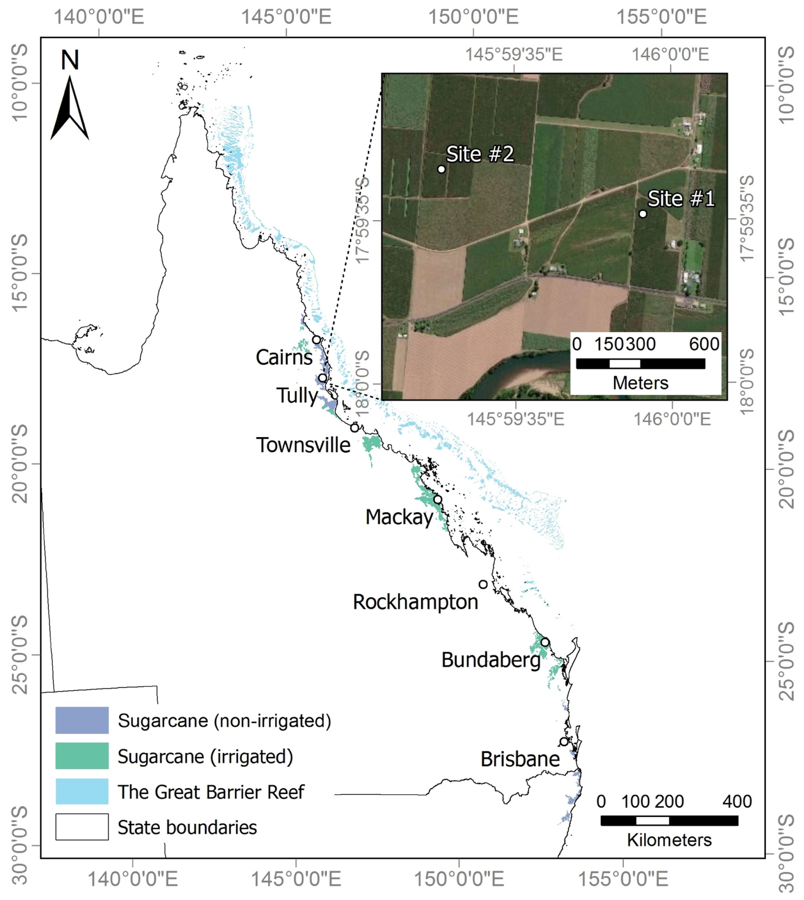
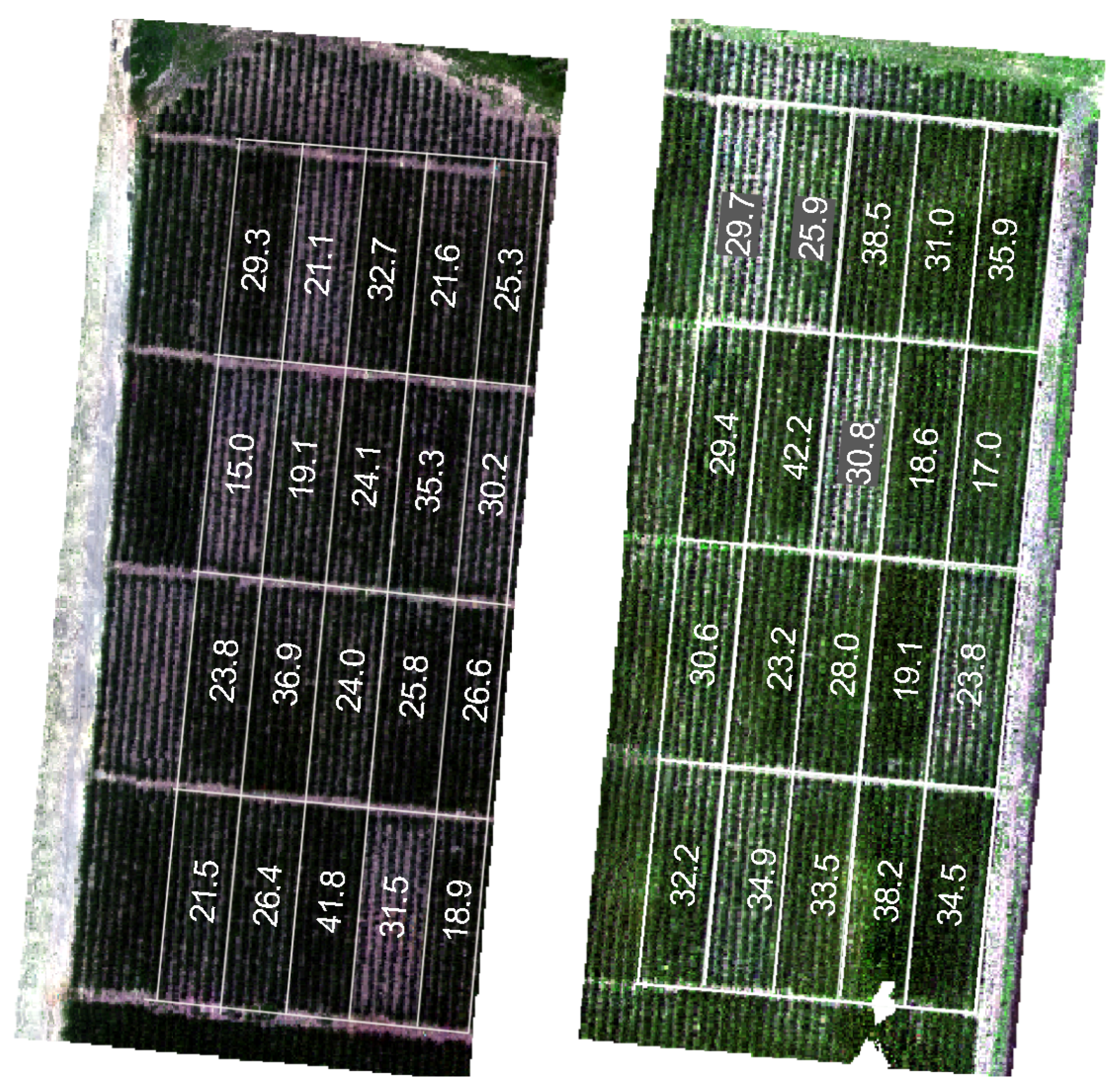
2.1. Study Area

The study area refers to the experiment described in the article written by Shendryk et al. [16], where the data were made available, and consists of two experimental fields, each measuring 1 hectare (ha), located in northeastern Australia (Figure 1). Both sites have an annual rainfall of over 4000 mm between December and March. Each experimental field (Figure 2) has different soil types, with Site #1 having well-drained alluvial soil and Site #2 having poorly drained alluvial soil.

The experimental design contained 5 Nitrogen (N) treatments at rates of 0, 70, 110, 150, and 190 kgN/ha, with four replicates in a Randomized Complete Block Design (Figure 2). Each block was 10 m wide, 30 m long, and had six sugarcane planting rows. The treatments were applied 52 and 55 days after the harvest of the previous crop in Site #1 and Site #2, respectively.

2.2. Dataset

The dataset comprises features from VIs and LiDAR data collected on six surveys. From VIs, at each survey, 70 features based on statistical measures like maximum, minimum, average, standard deviation, and percentiles (

Table 1. Feature names of statistical measures calculated from VIs of multispectral images [16].

Feature	Explanation
max	Maximum value of all pixels within each plot
min	Minimum value of all pixels within each plot
avg	Average value of all pixels within each plot
std	Standard deviation of all pixels within each plot
p25	25th percentile of all pixels within each plot
p50	50th percentile of all pixels within each plot
p75	75th percentile of all pixels within each plot

) calculated over the ten VIs shown in

Table 2. Vegetative indices and their equations based on the bands R: red, G: green, B: blue, NIR: near-infrared, RE: Red-edge.

Name	Equation
Normalized Difference Vegetation Index (NDVI) [19]	(NIR − R)/(NIR + R)
Normalized Difference Red Edge Index (NDRE) [20]	(NIR − RE)/(NIR + RE)
Green NDVI (GNDVI) [21]	(NIR − G)/(NIR + G)
Enhanced Vegetation Index (EVI) [22]	2.5(NIR − R)/(NIR + R) + 6R − 7.5B + 1
Modified Anthocyanin Content Index (MACI) [23]	NIR/G
Optimized Soil Adjusted Vegetation Index (OSAVI) [24]	(1 + 0.16) (NIR − R)/(NIR + R + 0.16)
Simplified Canopy Chlorophyll Content Index (SCCCI) [25]	NDRE/NDVI
Transformed Chlorophyll Absorption and Reflectance Index (TCARI) [26]	3[RE − R − 0.2(RE/G)(RE/R)]/OSAVI
Triangular Greenness Index (TGI) [27]	−0.5[(668 − 475)(R − G) − (668 − 560)(R − B)]
Visible Atmospherically Resistant Index (VARI) [28]	(G × R)/(G + R − B)

were used [16]. While LiDAR data are based on 48 statistical measures described in

Table 3. Feature names of statistical measures calculated from LiDAR data and their descriptions.

Feature	Explanation
max	maximum height
avg	average height
qav	quadratic average height
std	standard deviation of height
ske	height skewness
kur	height kurtosis
p05 to p95	5th to 95th height percentiles (increments of 5 percentiles)
b05 to b95	5th to 95th bicentiles a (increments of 5 percentiles)
d00	number of points between 0 (i.e., ground) and 0.01 m divided by the total number of points
d01 b	the number of points between 0.01 and 0.5 m divided by the total number of points
d02 b	the number of points between 0.5 and 1 m divided by the total number of points
d03 b	the number of points between 1 and 10 m divided by the total number of points

^a: fraction of points between ground and the height percentile. ^b: threshold values for d00, d01, d02, and d03 were defined to represent penetration of laser pulses at different height levels of sugarcane.

[16].

2.3. Proposed Approach

This study focuses on enhancing crop yield prediction for sugarcane using a combination of the VIs extracted from multispectral images, LiDAR data, and advanced regression techniques. Building on the experimental workflow of Shendryk et al. [16], adjustments were made to incorporate MFs derived from regressions based on statistical measures (Table 1 and Table 3) calculated from the features collected on the field (original predictor variables), Principal Component Analysis (PCA) [29], and other regressions. The workflow integrates various machine learning regressors, in addition to Linear Regression (LR), including Support Vector Regressor (SVR), Random Forest (RF), Gradient Boosting (GB), and AdaBoost (AB), along with a meta-regressor approach. These methods were systematically validated using ${\overline{R}}^2$ and RMSE (kg) metrics to assess predictive accuracy and model robustness.

In an attempt to improve the results presented in [16], some of the regressors presented in the sklearn [30] library of the Python 3.10.11 programming language were used:

• SVR: a generalization of Support Vector Machine (SVM) obtained by introducing a $\epsilon$-insensitive region around the function, called a $\epsilon$ tube. This tube reformulates the optimization problem to find the tube that best approximates the continuous-valued function while balancing model complexity and prediction error.
• RF regressor: a meta-estimator that fits some decision trees on multiple subsamples of the dataset and uses the average to improve predictive accuracy and control overfitting.
• GB regressor: estimator that builds an additive model progressively, allowing the optimization of arbitrary differentiable loss functions. At each stage, a regression tree is fitted on the negative gradient of the given loss function.
• AB regressor: is a meta-estimator that starts by fitting a regressor on the original dataset and then fits additional copies of the regressor on the same dataset, but where the weights of the instances are adjusted according to the error of the current prediction.

MFs were generated by transforming predicted values into new inputs for a meta-regressor, with AdaBoost demonstrating superior performance in predicting crop yield. Dimensionality reduction via PCA yielded five principal components, which were further processed to create 25 MFs. Among the tested models, those using the average NDVI (M1) of all pixels within each plot and combined multispectral and LiDAR data (M5) provided the most accurate predictions. All the models are described in

Table 4. Correspondence of models and the features they are based on.

Model	Features
M1	average NDVI (avg NDVI)
M2	maximum NDVI (max NDVI)
M3	Multispectral principal components ( MultispecPCs)
M4	LiDAR principal components (LiDARPCs)
M5	Multispectral + LiDAR principal components (MultispecPCs + LiDARPCs)
MF SVR M1…M5	Meta-feature extracted by SVR on M1…M5
MF RF M1…M5	Meta-feature extracted by RF on M1…M5
MF Grad Boost M1…M5	Meta-feature extracted by Gradient Boosting on M1…M5
MF AdaBoost M1…M5	Meta-feature extracted by AdaBoost on M1…M5
MF Linear Regression M1…M5	Meta-feature extracted by Linear Regression on M1…M5
MF kNN M1…M5	Meta-feature extracted by kNN on M1…M5

. The kNN regressor was also explored for improvements in chronological prediction, leveraging its proximity-based approach to enhance yield prediction. Hyperparameter tuning via Grid Search ensured optimal performance for each regressor, solidifying the workflow’s effectiveness in predicting crop yield.

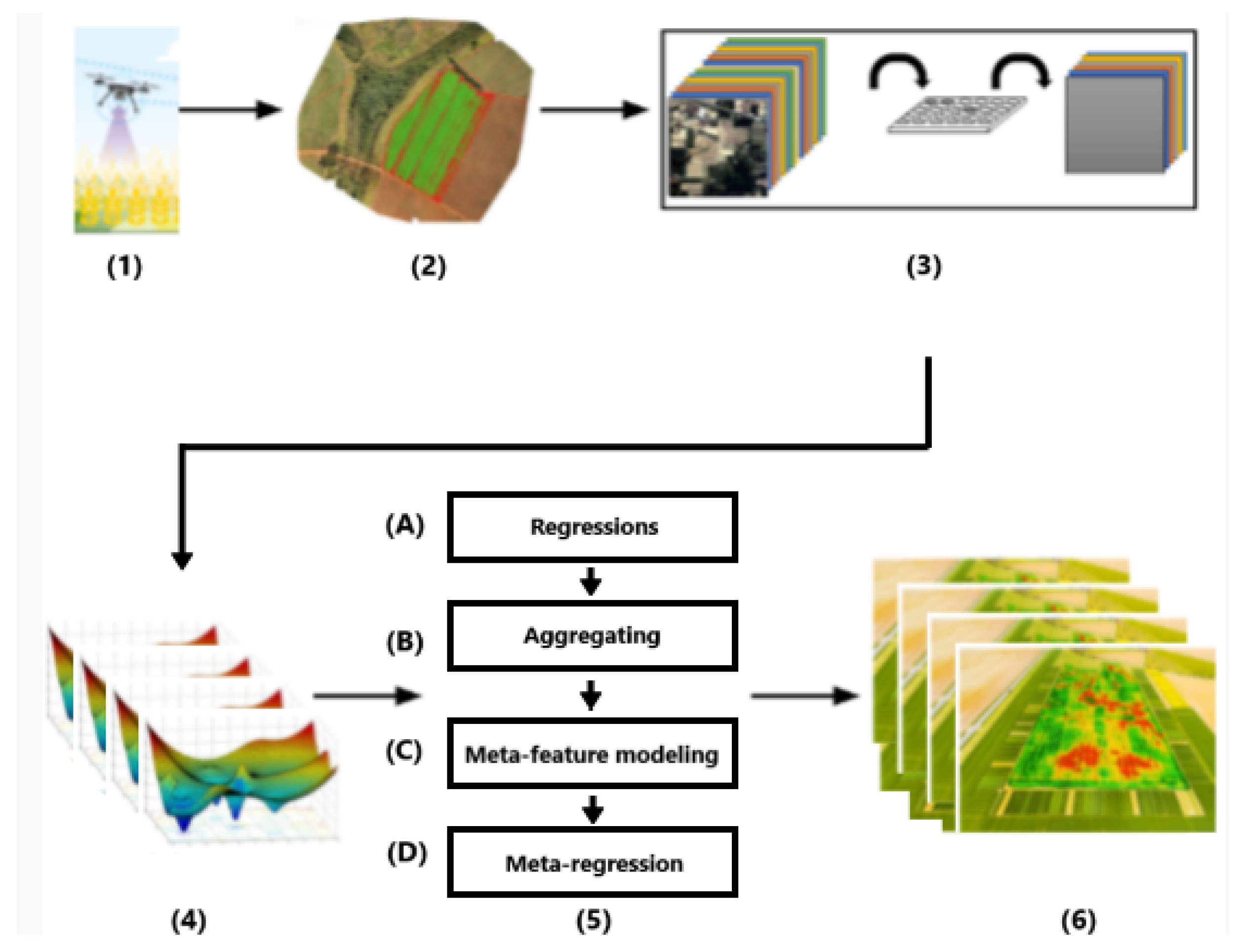
2.3.1. Crop Yield Prediction Workflow

This study was also conducted using the source code and dataset from two experimental sugarcane fields in Australia, made available in [16], which was enriched to incorporate the regressors SVR, RF, GB, and AB for evaluation from a meta-feature perspective. The experimental workflow established in [16] (illustrated in steps 1, 2, 3, 4, and 6 of Figure 3, without multiplicity for steps 4 and 6) was followed, enabling comparisons of results obtained with these regressors against those derived using LR.

2.3.2. Overview of Proposed Meta-Feature Approach

Figure 3, in step 5, illustrates the methodology adopted for incorporating MFs in a classical crop yield prediction workflow. As depicted in steps (1) to (6), the protocol involves capturing multispectral images and LiDAR data across six specific dates and collecting leaf and stalk samples from randomized locations within the experimental fields to assess nitrogen content and biomass levels. VIs were derived from the multispectral images, and statistical measures were calculated (Table 1). Similarly, the LiDAR data provided multiple statistical metrics (Table 3), offering a comprehensive dataset for subsequent analysis.

Let a meta-feature be a new representation of the sample in a new feature space; it can be defined as a vector of $\mathbf{d}$ dimensions (where $\mathbf{d}$ indicates the number of regressors considered), in which each dimension represents the prediction calculated by a regressor. Formally, the meta-feature vector can be defined as follows:

$$\mathbf{m}=\left(f_1\left(\mathbf{x}\right),f_2\left(\mathbf{x}\right),\dots ,f_d\left(\mathbf{x}\right)\right)$$

where

• $\mathbf{m}\in {\mathbb{R}}^d$ is the meta-feature vector;
• d is the number of regressors;
• $f_i\left(\mathbf{x}\right)$ is the prediction of the i-th regressor for the input sample $\mathbf{x}$.

2.3.3. Meta-Feature Modeling

From the original feature set, dimensionality reduction was performed, followed by feature modeling in which the reduced features were processed through various regressors. The predicted values from these regressors were then added to the dataset as MFs, resulting in a new synthetic dataset. Within this dataset, features derived from PCA and the MFs underwent further modeling. They were subsequently input into a meta-regressor, which generated multiple predictions to determine the optimal model, as illustrated in Figure 4.

In Figure 4, five models were selected based on statistical calculations of specific features (average NDVI and maximum NDVI), the principal components (MultispectralPCs and LiDARPCs), and a fusion of these two components (MultispectralPCs + LiDARPCs). These models were processed by each of the five regressors, producing a set of 25 MFs. These MFs were then integrated into the original dataset, and each, along with the five original features, was used as input to the meta-regressor AdaBoost, chosen for its superior ${\overline{R}}^2$ performance in [31], to predict crop yield.

2.3.4. Meta-Regressor by kNN

As an additional attempt to obtain even better performance for the crop yield prediction, the kNN regressor was used to generate other MFs, motivated by the best results achieved in [32,33]. After that, this regressor was applied to all feature models to improve prediction further. It was a form of having almost the exact crop yield on each data collection date.

Applying the kNN algorithm on a dataset directly reflects the quality of sample dispersion within the feature space, which is critical for its ability to distinguish between classes in classification tasks or predict values in regression tasks. The effectiveness of kNN relies on how well the samples are distributed in the feature space, with greater dispersion and distinctiveness typically leading to improved performance.

kNN’s advantage lies in its simplicity and effectiveness. It does not make strong assumptions about the data distribution, making it applicable to various datasets. Moreover, kNN can handle continuous and categorical data, making it versatile for many imputation scenarios. The choice to use kNN for imputation is often driven by the dataset’s nature and the need for a reliable and adaptable imputation method [34].

In the MF context, the feature space is often transformed through prior modeling steps, which can result in a more structured and well-distributed representation related to the original dataset. This enhanced distribution allows kNN to exploit the proximity relationships between samples more effectively, leading to more robust predictions. Furthermore, kNN’s sensitivity to local structures within the dataset makes it particularly suitable for leveraging the improved representation offered by MFs, enabling it to deliver accurate and reliable results.

2.3.5. Grid Search

Grid search optimizes hyperparameters to enhance model performance and systematically explores different values without human bias. This search was applied to select the most relevant hyperparameters for each regressor (SVR, RF, GB, and AB) and achieved optimal regression performance. This exhaustive search method explores a subset of a regressor’s hyperparameter space [35]. The selected hyperparameters for each regressor were used to predict crop yield across six surveys evaluated in [16].

Table 5. Hyperparameters used on each regressor applied.

Regressor	Hyperparameters
SVR	kernel = ’rbf’, C = 10, coef0 = 0.01, degree = 3, gamma = ’scale’
Random Forest	n_estimators = 200, max_features = ’sqrt’, max_depth = 3, random_state = 18
Gradient boosting	learning_rate = 0.01, max_depth = 4, n_estimators = 100, subsample = 0.5
AdaBoost	learning_rate = 0.1, loss = ’exponential’, n_estimators = 50

presents the hyperparameters used and their respective values.

2.4. Experimental Evaluation

2.4.1. Baseline Methods

The regression modeling approach adhered to the methodology outlined in [7], where multiple regressors were evaluated and tuned for optimal performance using the Grid Search algorithm [35] to adjust hyperparameters. A diverse set of regressors was assessed on a dataset comprising two experimental sugarcane fields from Australia, sourced from [16], to predict crop yield for comparative analysis with the Ordinary Least Squares (OLS) method documented in the same study. Prior findings, as presented in [31], indicated that LR did not achieve results as significant as those observed in SVR, RF, GB, and AB, with top-performing values summarized in

Table 6. Summarization of average values of ${\overline{R}}^2$ for the different models obtained from the regressors evaluated in this work.

Regressors	avgNDVI	maxNDVI	LiDARPCs	MultispecPCs	MultispecPCs + LiDARPCs
LR	0.17	0.18	0.40	0.42	0.39
SVR	0.52	0.48	0.63	0.64	0.39
Random Forest	0.52	0.48	0.63	0.62	0.30
Gradient Boosting	0.51	0.49	0.49	0.54	0.00
Ada Boost	0.51	0.50	0.64	0.65	0.50

.

2.4.2. Experimental Protocol

The source code of [16] was modified to incorporate other regressors and compare their results with those obtained using the original dataset. The dataset was then separated into subsets for training and testing at a ratio of 0.8:0.2, respectively.

Contrary to the result of the crop yield predict presented in work [16], it was possible to improve the ${\overline{R}}^2$ (described in Equation (1)) for all samples and all models used in it, except the Random Forest and Gradient Boosting regressors, which did not have good results for the Multispectral + LiDAR model.

$${\overline{R}}^2=1-(1-R^2)\ast ((n-1)/(n-p-1))$$

(1)

where

• R²: R-squared value for a linear regression (described in Equation (2));
• n: sample size used in regression;
• p: number of predictors used in the regression, including the constant.

$$R^2=1-{\displaystyle \frac{{\sum }_{i=1}^n{(y_i-{\widehat{y}}_i)}^2}{{\sum }_{i=1}^n{(y_i-\overline{y})}^2}}$$

(2)

where

• $y_i$: observed value;
• ${\widehat{y}}_i$: predicted value from the model;
• $\overline{y}$: mean of the observed values;
• n: total number of observations.

3. Results

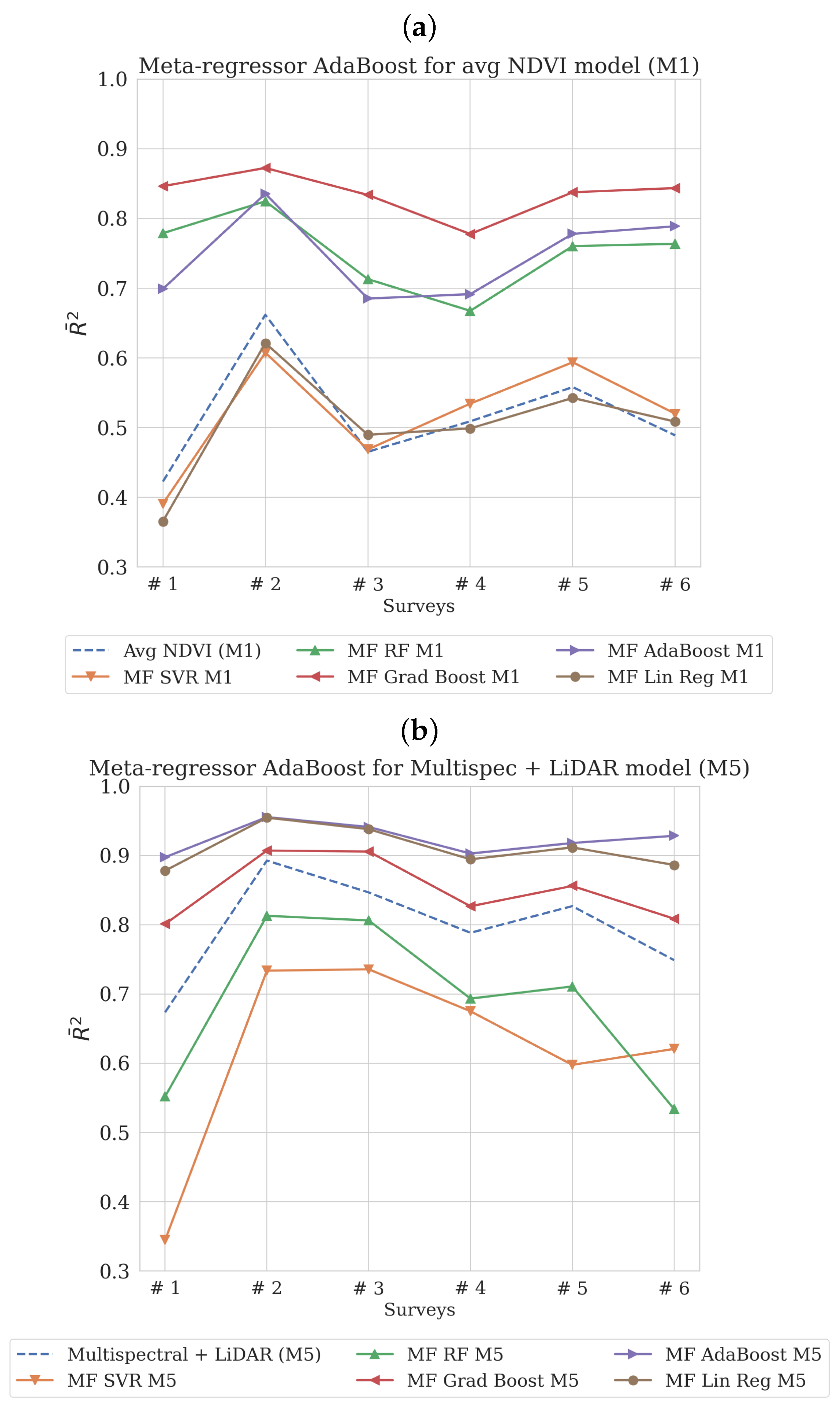
3.1. Prelimenary Results

The MFs are generated by applying each regressor (LR, SVR, RF, GB, and AB) to each model from M1 to M5, as described in Table 4. These regressors were selected based on findings in the literature [36,37]. The combinations of these regressors and features align with models previously used for predictions with the original dataset at [16]. They were already utilized in [31]. This approach yielded even better performance when compared to the original model, with an average ${\overline{R}}^2$ across samples exceeding 0.9, as illustrated in Figure 5a and Figure 5b, respectively for M1 and M5.

After data analysis, the two most effective combinations across the six acquisition dates (surveys), in terms of highest ${\overline{R}}^2$ and lowest RMSE, were identified as Average NDVI (M1) and the combination of Multispectral and LiDAR data (M5), as illustrated in Figure 5. A higher ${\overline{R}}^2$ value indicates a more robust predictive performance, making these combinations the top choices.

The RMSE values (Figure 6a,b, respectively for M1 and M5) calculated for these regressions were consistent with ${\overline{R}}^2$ results across the six dates; a lower RMSE (kg) value indicates a more robust model performance.

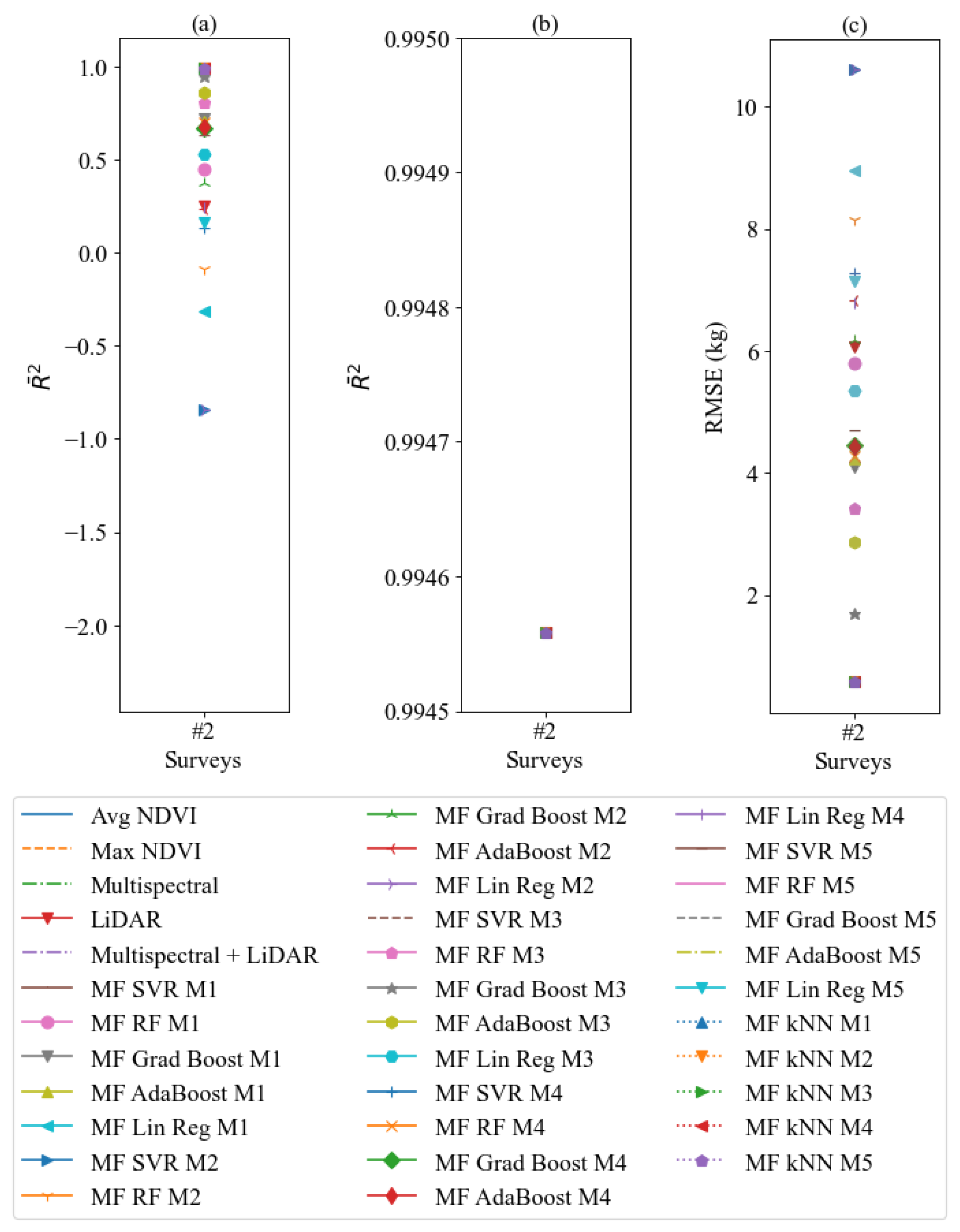
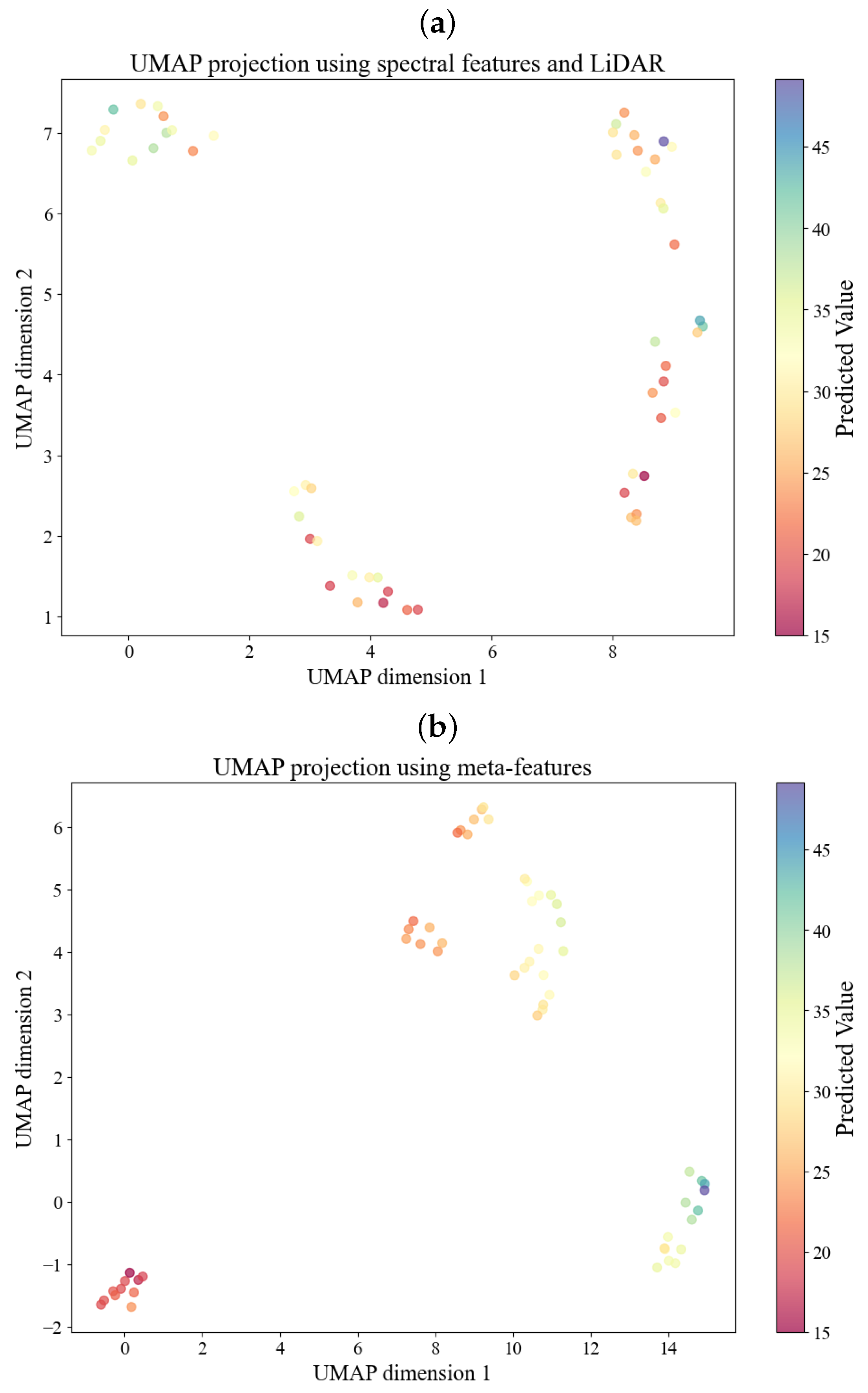
3.2. Results by Meta-Features Produced from kNN Meta-Regressor

To verify the hypothesis that additional MFs generated using a kNN regressor would improve the prediction, they were generated using this regressor [30], which was also employed as a new meta-regressor. This approach produced five new models: MF kNN M1, MF kNN M2, MF kNN M3, MF kNN M4, MF kNN M5; for example, MF kNN M1 is the meta-feature obtained by the regressor kNN applied to the M1 feature model (composed by Avg NDVI), and MF kNN M5 is the meta-feature obtained by the regressor kNN applied to the M5 feature model (composed by MultispecPCs + LiDARPCs). Therefore, the meta-regressor AdaBoost was employed on the features already used, plus the MFs produced by the kNNRegressor, illustrated by Figure 7, which improved the performance. For clarity, the results are only presented for the second survey. As advantages, first, this date already gave the best results (Figure 5), which provide a challenging context to verify how our approach may improve the prediction, second, the acquisition date is well before harvest and constitutes an example on how the methodology may perform relevant yield prediction long before harvest.

After, showed in Figure 8, applying the kNN regressor as a meta-regressor yielded only excellent results, for feature models based on MFs, to those obtained using AdaBoost regressor, but with some negative values of ${\overline{R}}^2$ and RMSE varying from more than 1 kg to more than 10 kg (for AdaBoost meta-regressor it is from less than 1 kg to less than 5 kg), with the lowest performance observed in the models MF Lin Reg M1, MF SVR M2, and MF RF M2. This indicates that the kNN regressor produced good MFs and outperformed AdaBoost as a meta-regressor in terms of ${\overline{R}}^2$ but not in terms of RMSE. The comparison is shown in

Table 7. Comparison between the baseline (the first five feature models) and proposed method and approach (based on MFs) of ${\overline{R}}^2$ and RMSE for kNN and AdaBoost regressors.

Feature Model	${\overline{\mathit{R}}}^2$ kNN	${\overline{\mathit{R}}}^2$ AdaBoost	RMSE kNN	RMSE AdaBoost
Avg NDVI	−0.3135	0.2370	8.9590	6.8284
Max NDVI	−0.8407	−0.1465	10.6058	8.3700
Multispectral	−0.1451	0.3187	6.9988	5.3984
LiDAR	0.2498	0.6571	6.0561	4.0943
Multispectral + LiDAR	−2.2980	0.0281	8.9785	4.8742
MF SVR M1	−0.3135	0.1771	8.9590	7.0911
MF RF M1	0.4488	0.5311	5.8035	5.3530
MF Grad Boost M1	0.7252	0.7211	4.0977	4.1282
MF AdaBoost M1	0.7076	0.7139	4.2273	4.1810
MF Lin Reg M1	−0.3135	0.1719	8.9590	7.1138
MF SVR M2	−0.8407	−0.1821	10.6058	8.4991
MF RF M2	−0.0839	0.1841	8.1385	7.0612
MF Grad Boost M2	0.3780	0.6091	6.1654	4.8876
MF AdaBoost M2	0.2388	0.5683	6.8201	5.1362
MF Lin Reg M2	−0.8407	−0.1776	10.6058	8.4831
MF SVR M3	0.7272	0.8462	4.0833	3.0658
MF RF M3	0.8081	0.9067	3.4245	2.3881
MF Grad Boost M3	0.9528	0.9406	1.6985	1.9046
MF AdaBoost M3	0.8651	0.9044	2.8710	2.4165
MF Lin Reg M3	0.5331	0.5851	5.3413	5.0352
MF SVR M4	0.1326	0.5767	7.2803	5.0857
MF RF M4	0.7022	0.7868	4.2659	3.6096
MF Grad Boost M4	0.6744	0.8037	4.4607	3.4634
MF AdaBoost M4	0.6797	0.7692	4.4238	3.7558
MF Lin Reg M4	0.2458	0.5674	6.7888	5.1414
MF SVR M5	0.6388	0.8150	4.6980	3.3627
MF RF M5	0.8183	0.8060	3.3323	3.4435
MF Grad Boost M5	0.9452	0.9460	1.8294	1.8169
MF AdaBoost M5	0.8701	0.9235	2.8171	2.1621
MF Lin Reg M5	0.1682	0.5218	7.1294	5.4055
MF kNN M1	0.9946	0.9906	0.5766	0.7575
MF kNN M2	0.9946	0.9881	0.5766	0.8532
MF kNN M3	0.9946	0.9884	0.5766	0.8436
MF kNN M4	0.9946	0.9908	0.5766	0.7514
MF kNN M5	0.9946	0.9852	0.5766	0.9502

to clarify the differences, and Figure 9 illustrates the harvest quantities in each plot during survey #2.

Using kNN-derived MFs yielded superior results in ${\overline{R}}^2$ and RMSE, suggesting that the kNN regressor is a promising choice. Consequently, it was applied as a meta-regressor across all available models (including the original models M1, M2, M3, M4, and M5, as well as all MF models) to enhance further the results achieved with the AdaBoost meta-regressor. Figure 8 illustrates that the models based on MF kNN achieve an ${\overline{R}}^2$ value around 0.99 across nearly all instances and dates, except for models MF AdaBoost M1, M2, M3, M4, and M5.

These findings demonstrate the effectiveness of incorporating meta-features generated by a kNN regressor, particularly when used in conjunction with an AdaBoost meta-regressor, resulting in substantial improvements in both ${\overline{R}}^2$ and RMSE. Although the kNN regressor also showed promise as a standalone meta-regressor—especially in terms of ${\overline{R}}^2$—its performance in RMSE was comparatively inferior to that of AdaBoost. Using kNN-generated meta-features combined with AdaBoost as the meta-regressor led to consistently high predictive performance, with ${\overline{R}}^2$ values nearing 0.99 in most configurations. These results point to the effectiveness of combining meta-feature construction with ensemble learning to strengthen model accuracy in yield prediction tasks. This strategy shows particular promise for generating reliable forecasts well ahead of harvest. Further investigation is needed to assess how well the approach performs when applied to other crops, environmental conditions, and types of input features.

4. Discussion

A substantial contribution to this study is using MF based on regressions made from features with multispectral and LiDAR data to predict crop yields. Other works in the literature normally use VIs, soil data, meteorology data, management through remote sensing data collected by satellite or UAVs, and proximity sensors, but do not take advantage of the potential provided by MFs. Bringing MFs and meta-regression is a way of reusing a dataset to explore new possibilities.

The results of this study demonstrate that applying novel strategies for generating MFs enhances crop yield prediction accuracy at least for sugarcane in this experiment. This approach enables a more comprehensive exploration of the dataset’s informational potential. Beyond traditional statistical operations, such as calculating averages, maxima, minima, standard deviations, and quartiles, aggregating new MFs can yield better outcomes, enriching the dataset for improved predictive performance.

Adding a new set of MFs extracted from the kNN regressor applied to all the original models showed that this technique improves crop yield prediction and can be explored incrementally. Similarly, the new meta-regressors that predict biomass are also efficient when applied to crop yield.

To assess whether, through a regressor based on the kNN of each sample, crop yield is achieved with similar values, a scatter plot was created with the projection of data in two dimensions (Figure 10) using the UMAP algorithm [38], a widely used method for dimensionality reduction that allows the visualization of complex relationships and patterns in high-dimensional datasets. In Figure 10, the color of the points in space represents the value of the crop yield prediction obtained from the regression of all the features, original features (a), and MFs (b), using KNeighborsRegressor [30]. The projections were made by using the features involved in the original modeling from M1 to M5 (avg NDVI, max NDVI, MultispecPCs, LiDARPCs, and MultispecPCs + LiDARPCs, respectively) in projection 1 and using the MFs (produced from regressors SVR, RF, GB, AB, LR, and kNN applied on the models from M1 to M5) in projection 2.

In Figure 10a, the features used to make the prediction directly impact the data organization in the projected space and do not optimize the separation of points with proximity of similar predicted values; the projection generated shows a significant dispersion of points, without a clear definition of similarity. This observed dispersion suggests that the features have a less direct relationship with the predicted value. The absence of similarity patterns between M1 and M5 (a), in contrast to MFs (b), where similar conditions can be observed, suggests that models M1 to M5 may capture more continuous or heterogeneous patterns that do not naturally divide the projected space.

Figure 10b shows a precise formation of well-defined similarity points. Almost all grouped points share the same color, indicating more uniformity in the predicted value. This suggests that the MF significantly improves the relationship with the response variable. The uniformity in coloring within each group of points suggests that the predicted values are consistent, reinforcing that the MF captures patterns directly related to the response variable.

At least in Figure 10b, UMAP organized the features to maximize group separation, reflecting a clear correspondence between the features and the predicted values. It is also important to emphasize that the dispersion in projection 1 does not mean that the features are irrelevant; they have more complex relationships with the response variable.

The UMAP approach to visualization is beneficial in agricultural contexts, where analyzing VIs and LiDAR data can be challenging. UMAP allows us to understand the relationships between samples and their predictions.

The kNN regressor was selected as the meta-regressor due to its strong dependence on the structure and relevance of input features. As a non-parametric, instance-based learner, kNN makes predictions based on the similarity of data points in the feature space, making it highly responsive to the quality of the meta-features produced by base models. This characteristic renders kNN particularly effective for assessing and leveraging meta-features in ensemble learning settings. The influence of these meta-features on the performance of the kNN regressor is further analyzed and visualized in Figure 10b.

Using MFs and meta-regressors can yield even better results for crop yield prediction. This technique may leverage different aspects of the same dataset, thereby increasing its potential for use without requiring new surveys. It also enhances prediction performance using a method not previously explored in the literature, providing additional possibilities to evaluate several datasets already collected. By exploiting this type of data, prediction models for different crops can be optimized without collecting additional field data.

As part of future work, we propose extending this study through large-scale analyses involving significantly more samples to understand better the generalization capacity of the meta-regressor under varying data distributions. Furthermore, to enhance the performance of the kNN-based meta-regressor, we suggest investigating advanced strategies such as re-ranking mechanisms. Re-ranking has shown promise in improving the effectiveness of kNN by refining neighborhood structures through manifold learning and contextual similarity adjustments. Recent research has shown that modifying initial kNN outputs using local or global contextual information can significantly improve performance in retrieval and classification tasks [39,40]. Adapting such techniques to regression settings may improve prediction accuracy and robustness in meta-learning frameworks.

Future work should also include performance improvements and thoroughly evaluate the proposed approach’s computational efficiency. While the kNN meta-regressor’s predictive accuracy is promising, its computational cost—particularly in high-dimensional spaces and large datasets—may pose scalability challenges.

5. Conclusions

Exploring datasets beyond traditional statistical tools (e.g., averages, maxima, minima, standard deviation, and quartiles) and incorporating different regressors after dimensionality reduction techniques can significantly enhance ${\overline{R}}^2$ and RMSE outcomes. MFs derived from regressions, particularly MF Grad Boost and MF AdaBoost obtained from M1 (average NDVI) and M5 (MultispectralPCs + LiDARPCs) models, outperformed original predictions, delivering superior results. Using kNN MFs under the AdaBoost meta-regressor and then applying the kNN meta-regressor yielded even better results.

This study demonstrated the value of MFs and meta-regressors in improving sugarcane crop yield prediction without requiring additional data collection. The method enhances predictive accuracy and identifies optimal models by augmenting original datasets with MFs and systematically evaluating regressors. This approach not only refines existing data but also supports better decision-making for harvesting logistics and optimizes agricultural management practices.

References

1. Van Klompenburg, T.; Kassahun, A.; Catal, C. Crop yield prediction using machine learning: A systematic literature review. Comput. Electron. Agric. 2020, 177, 105709. [Google Scholar] [CrossRef]
2. Amarasingam, N.; Salgadoe, A.S.A.; Powell, K.; Gonzalez, L.F.; Natarajan, S. A review of UAV platforms, sensors, and applications for monitoring of sugarcane crops. Remote Sens. Appl. Soc. Environ. 2022, 26, 100712. [Google Scholar] [CrossRef]
3. Nogueira, E.A.; Felix, J.P.; Fonseca, A.U.; Vieira, G.; Ferreira, J.C.; Fernandes, D.S.; Oliveira, B.M.; Soares, F. Deep Learning for Super Resolution of Sugarcane Crop Line Imagery from Unmanned Aerial Vehicles. In Advances in Visual Computing, Proceedings of the 18th International Symposium, ISVC 2023, Lake Tahoe, NV, USA, 16–18 October 2023; Springer: Cham, Switzerland, 2023; pp. 597–609. [Google Scholar] [CrossRef]
4. Ribeiro, J.B.; da Silva, R.R.; Dias, J.D.; Escarpinati, M.C.; Backes, A.R. Automated detection of sugarcane crop lines from UAV images using deep learning. Inf. Process. Agric. 2024, 11, 385–396. [Google Scholar] [CrossRef]
5. De França e Silva, N.R.; Chaves, M.E.D.; Luciano, A.C.d.S.; Sanches, I.D.; de Almeida, C.M.; Adami, M. Sugarcane yield estimation using satellite remote sensing data in empirical or mechanistic modeling: A systematic review. Remote Sens. 2024, 16, 863. [Google Scholar] [CrossRef]
6. Arakawa, K.; Shimizu, R.; Kikuchi, S.; Capi, G. Sugar Cane Yield Prediction Using Drone Data Processed by LSTM Algorithm. In Proceedings of the 2025 3rd International Conference on Mechatronics, Control and Robotics (ICMCR), Singapore, 14–16 February 2025; IEEE: Piscataway, NJ, USA, 2025; pp. 75–79. [Google Scholar] [CrossRef]
7. Afraei, S.; Shahriar, K.; Madani, S.H. Statistical assessment of rock burst potential and contributions of considered predictor variables in the task. Tunn. Undergr. Space Technol. 2018, 72, 250–271. [Google Scholar] [CrossRef]
8. Bessa, A.D. Explaining and Identifying Data to Support Data-Driven Analyses. Ph.D Thesis, Tandon School of Engineering, New York University, New York, NY, USA, 2020. Available online: https://www.proquest.com/openview/d114405d255b4cf22737514bb01ca748/1?cbl=18750&diss=y&pq-origsite=gscholar (accessed on 2 March 2025).
9. Akbarian, S.; Xu, C.; Wang, W.; Ginns, S.; Lim, S. An investigation on the best-fit models for sugarcane biomass estimation by linear mixed-effect modelling on unmanned aerial vehicle-based multispectral images: A case study of Australia. Inf. Process. Agric. 2023, 10.3, 361–376. [Google Scholar] [CrossRef]
10. Sarkar, S.; Dey, A.; Pradhan, R.; Sarkar, U.M.; Chatterjee, C.; Mondal, A.; Mitra, P. Crop Yield Prediction Using Multimodal Meta-Transformer and Temporal Graph Neural Networks. IEEE Trans. Agrifood Electron. 2024, 2, 545–553. [Google Scholar] [CrossRef]
11. Bansal, Y.; Lillis, D.; Kechadi, M.T. A neural meta model for predicting winter wheat crop yield. Mach. Learn. 2024, 113, 3771–3788. [Google Scholar] [CrossRef]
12. Ermolieva, T.; Havlik, P.; Lessa-Derci-Augustynczik, A.; Boere, E.; Frank, S.; Kahil, T.; Wang, G.; Balkovic, J.; Skalsky, R.; Folberth, C.; et al. A novel robust meta-model framework for predicting crop yield probability distributions using multisource data. Cybern. Syst. Anal. 2023, 59, 844–858. [Google Scholar] [CrossRef]
13. Tunio, M.H.; Li, J.P.; Zeng, X.; Akhtar, F.; Shah, S.A.; Ahmed, A.; Yang, Y.; Heyat, M.B.B. Meta-knowledge guided Bayesian optimization framework for robust crop yield estimation. J. King Saud Univ.-Comput. Inf. Sci. 2024, 36, 101895. [Google Scholar] [CrossRef]
14. Anbananthen, K.S.M.; Subbiah, S.; Chelliah, D.; Sivakumar, P.; Somasundaram, V.; Velshankar, K.H.; Khan, M.A. An intelligent decision support system for crop yield prediction using hybrid machine learning algorithms. F1000Research 2021, 10, 1143. [Google Scholar] [CrossRef] [PubMed]
15. Joshaghani, M.; Barak, S.; Asadi, A.; Mirafzali, E. Retail Time Series Forecasting Using An Automated Deep Meta-Learning Framework. SSRN Electron. J. 2023. [Google Scholar] [CrossRef]
16. Shendryk, Y.; Sofonia, J.; Garrard, R.; Rist, Y.; Skocaj, D.; Thorburn, P. Fine-scale prediction of biomass and leaf nitrogen content in sugarcane using UAV LiDAR and multispectral imaging. Int. J. Appl. Earth Obs. Geoinf. 2020, 92, 102177. [Google Scholar] [CrossRef]
17. James, G.; Witten, D.; Hastie, T.; Tibshirani, R.; Taylor, J. An Introduction to Statistical Learning; Springer: Cham, Switzerland, 2023; Volume 112. [Google Scholar] [CrossRef]
18. Barbosa, L.A.F.; Pedronette, D.C.G.; Guilherme, I.R. A Meta-Feature Model for Exploiting Different Regressors to Estimate Sugarcane Crop Yield. In Proceedings of the IGARSS 2023–2023 IEEE International Geoscience and Remote Sensing Symposium, Pasadena, CA, USA, 16–21 July 2023; pp. 2030–2033. [Google Scholar] [CrossRef]
19. Rouse, J.W., Jr.; Haas, R.H.; Schell, J.A.; Deering, D.W. Monitoring Vegetation Systems in the Great Plains with ERTS. In Proceedings of the Third Earth Resources Technology Satellite-1 Symposium, Washington, DC, USA, 10–14 December 1973; NASA/Goddard Space Flight Center: Greenbelt, MD, USA, 1973; pp. 309–317. Available online: https://ntrs.nasa.gov/citations/19740022614 (accessed on 2 March 2025).
20. Sims, D.A.; Gamon, J.A. Relationships between leaf pigment content and spectral reflectance across a wide range of species, leaf structures and developmental stages. Remote Sens. Environ. 2002, 81, 337–354. [Google Scholar] [CrossRef]
21. Gitelson, A.A.; Kaufman, Y.J.; Merzlyak, M.N. Use of a Green Channel in Remote Sensing of Global Vegetation From EOS-MODIS. Remote Sens. Environ. 1996, 58, 289–298. [Google Scholar] [CrossRef]
22. Evett, I.; Jackson, G.; Lambert, J.; McCrossan, S. The impact of the principles of evidence interpretation on the structure and content of statements. Sci. Justice 2000, 40, 233–239. [Google Scholar] [CrossRef] [PubMed]
23. Steele, M.R.; Gitelson, A.A.; Rundquist, D.C.; Merzlyak, M.N. Nondestructive estimation of anthocyanin content in grapevine leaves. Am. J. Enol. Vitic. 2009, 60, 87–92. [Google Scholar] [CrossRef]
24. Rondeaux, G.; Steven, M.; Baret, F. Optimization of Soil-Adjusted Vegetation Indices. Remote Sens. Environ. 1996, 55, 95–107. [Google Scholar] [CrossRef]
25. Barnes, E.; Clarke, T.; Richards, S.; Colaizzi, P.; Haberland, J.; Kostrzewski, M.; Waller, P.; Choi, C.; Riley, E.; Thompson, T.; et al. Coincident detection of crop water stress, nitrogen status and canopy density using ground based multispectral data. In Proceedings of the Fifth International Conference on Precision Agriculture, Bloomington, MN, USA, 16–19 July 2000; Volume 1619. Available online: https://www.tucson.ars.ag.gov/unit/Publications/PDFfiles/1356.pdf (accessed on 2 March 2025).
26. Hess, K.W.; Schmalz, R.A.; Zervas, C.E.; Collier, W. Tidal Constituent and Residual Interpolation (TCARI): A New Method for the Tidal Correction of Bathymetric Data. 1999. Available online: https://repository.library.noaa.gov/view/noaa/1689/noaa_DS1_1689.pdf (accessed on 2 March 2025).
27. Hunt, E.R., Jr.; Daughtry, C.; Eitel, J.U.; Long, D.S. Remote sensing leaf chlorophyll content using a visible band index. Agron. J. 2011, 103, 1090–1099. [Google Scholar] [CrossRef]
28. Gitelson, A.A.; Stark, R.; Grits, U.; Rundquist, D.; Kaufman, Y.; Derry, D. Vegetation and soil lines in visible spectral space: A concept and technique for remote estimation of vegetation fraction. Int. J. Remote Sens. 2002, 23, 2537–2562. [Google Scholar] [CrossRef]
29. Hotelling, H. Analysis of a complex of statistical variables into principal components. J. Educ. Psychol. 1933, 24, 417–441. [Google Scholar] [CrossRef]
30. Pedregosa, F.; Varoquaux, G.; Gramfort, A.; Michel, V.; Thirion, B.; Grisel, O.; Blondel, M.; Prettenhofer, P.; Weiss, R.; Dubourg, V.; et al. Scikit-learn: Machine learning in Python. J. Mach. Learn. Res. 2011, 12, 2825–2830. Available online: https://www.jmlr.org/papers/volume12/pedregosa11a/pedregosa11a.pdf?source=post_page (accessed on 2 March 2025).
31. Barbosa, L.A.F.; Pedronette, D.C.G.; Guilherme, I.R. Estudo comparativo entre diferentes regressores para estimar produtividade de cana-de-açúcar. SBSR-Simpósio Bras. Sensoriamento Remoto 2023, 20, 1020–1023. Available online: http://marte2.sid.inpe.br/col/sid.inpe.br/marte2/2023/04.30.20.56/doc/155771.pdf (accessed on 2 March 2025).
32. Cosenza, D.N.; Korhonen, L.; Maltamo, M.; Packalen, P.; Strunk, J.L.; Næsset, E.; Gobakken, T.; Soares, P.; Tomé, M. Comparison of linear regression, k-nearest neighbour and random forest methods in airborne laser-scanning-based prediction of growing stock. For. Int. J. For. Res. 2020, 94, 311–323. [Google Scholar] [CrossRef]
33. Malhotra, K.; Mishra, D.; Tumrate, C.S. Prediction of concrete compressive strength employing machine learning techniques. Mater. Today Proc. 2023, in press. [Google Scholar] [CrossRef]
34. Venkatesh, T.; Livingston, J.; Rajkumar, S. A Predictive Model for Marine Debris Prediction (A Comparative Case Study). In Proceedings of the 2024 Second International Conference on Emerging Trends in Information Technology and Engineering (ICETITE), Vellore, India, 22–23 February 2024; IEEE: Piscataway, NJ, USA, 2024; pp. 1–7. [Google Scholar] [CrossRef]
35. Ippolito, P.P. Hyperparameter Tuning: The Art of Fine-Tuning Machine and Deep Learning Models to Improve Metric Results. In Applied Data Science in Tourism: Interdisciplinary Approaches, Methodologies, and Applications; Springer: Berlin/Heidelberg, Germany, 2022; pp. 231–251. [Google Scholar] [CrossRef]
36. Zhang, Y.; Liu, J.; Shen, W. A review of ensemble learning algorithms used in remote sensing applications. Appl. Sci. 2022, 12, 8654. [Google Scholar] [CrossRef]
37. Tahaseen, M.; Moparthi, N.R. An Assessment of the Machine Learning Algorithms Used in Agriculture. In Proceedings of the 2021 5th International Conference on Electronics, Communication and Aerospace Technology (ICECA), Coimbatore, India, 2–4 December 2021; IEEE: Piscataway, NJ, USA, 2021; pp. 1579–1584. [Google Scholar] [CrossRef]
38. McInnes, L.; Healy, J.; Melville, J. Umap: Uniform manifold approximation and projection for dimension reduction. arXiv 2018, arXiv:1802.03426. [Google Scholar] [CrossRef]
39. De Antonio, A.L.T.; Pedronette, D.C.G. Manifold Learning for Brain Tumor MRI Image Retrieval and Classification. In Proceedings of the 2023 IEEE 23rd International Conference on Bioinformatics and Bioengineering (BIBE), Dayton, OH, USA, 4–6 December 2023; IEEE: Piscataway, NJ, USA, 2023; pp. 36–42. [Google Scholar] [CrossRef]
40. Gonçalves, F.M.F.; Pedronette, D.C.G.; da Silva Torres, R. Regression by re-ranking. Pattern Recognit. 2023, 140, 109577. [Google Scholar] [CrossRef]
Figure 1. Location of experimental fields that specify experimental fields, described as Site #1 and Site #2, and the areas where sugarcane is cultivated under irrigation or not in the big map, despite the irrigation not being treated in this paper [16].
Remotesensing 17 01846 g001
Figure 2. Experimental design containing biomass (2 m × 2 m area randomly positioned in each plot) and nitrogen collection points, and the amount of nitrogen applied to each plot represented by the numerical values [16].
Remotesensing 17 01846 g002
Figure 3. Workflow for obtaining crop yield prediction from VIs and LiDAR extracted from images captured at time t with UAV using the steps: (1) acquisition of multispectral and LiDAR data using UAV technology; (2) calculation of 10 VIs from multispectral imagery; (3) dimensionality reduction of features using PCA; (4) development of crop yield prediction models from VIs, optimized through hyperparameter tuning with Grid Search [31]; (6) evaluation and comparison of the models to determine the best-performing approach. The most important step in incorporating MFs into this study’s protocol is (5). At this point, (A) the regressions (SVR, RF, GB, AB, and LR) produced results; (B) they were aggregated to the original dataset as new features, the MFs; (C) these MFs were modeled independently; (D) they were submitted to the meta-regressor, which obtained the best performance, as detailed in Figure 4.
Remotesensing 17 01846 g003
Figure 4. Detailed visualization of step 5 from Figure 3 defined by the dimensional reduction of the dataset followed by the following: (1) the different regressions; (2) the aggregation of regressions as new MFs; (3) the use of each meta-feature as a new model; (4) the meta-regression for obtaining crop yield prediction.
Remotesensing 17 01846 g004
Figure 5. Charts containing the original model (a) avg NDVI (M1) and (b) Multispectral + LiDAR (M5)—dashed lines—and those models produced from MFs based on the regressors used in [7] for those same models. It shows that model MF Grad Boost (M1) and MF AdaBoost (M5) have the highest values for R ¯ 2 , telling how well this predictor can explain the crop yield.
Remotesensing 17 01846 g005
Figure 6. RMSE calculated for models M1 (a), M5 (b)—dashed lines —, and those models produced from MFs based on the regressors used in [31] for those same models.
Remotesensing 17 01846 g006
Figure 7. Charts containing the kNN MF under AdaBoost meta-regressor with MF extracted by kNNRegressor.
Remotesensing 17 01846 g007
Figure 8. Charts also containing the kNN MF under the kNN meta-regressor.
Remotesensing 17 01846 g008
Figure 9. Site #1 and site #2 during survey #2 with the amount harvested per plot.
Remotesensing 17 01846 g009
Figure 10. Uniform Manifold Approximation and Projection considering (a) features used in models from M1 to M5, and (b) in models produced by MFs. Each point in (a,b) represents one plot in Site #1 and #2, and its colors represent the predicted value of the plot. The two dimensions created, UMAP dimension 1 and UMAP dimension 2, represent new axes in a transformed space. These axes do not correspond to specific features but are defined by the UMAP technique. When the projection is applied to MFs, it becomes easier to identify nearby points and perceive patterns of similarity between points in the image corresponding to points with similar colors.
Remotesensing 17 01846 g010