Detail and Deep Feature Multi-Branch Fusion Network for High-Resolution Farmland Remote-Sensing Segmentation

Abstract

Currently, the demand for refined crop monitoring through remote sensing is increasing rapidly. Due to the similar spectral and morphological characteristics of different crops and vegetation, traditional methods often rely on deeper neural networks to extract meaningful features. However, deeper networks face a key challenge: while extracting deep features, they often lose some boundary details and small-plot characteristics, leading to inaccurate farmland boundary classifications. To address this issue, we propose the Detail and Deep Feature Multi-Branch Fusion Network for High-Resolution Farmland Remote-Sensing Segmentation (DFBNet). DFBNet introduces an new three-branch structure based on the traditional UNet. This structure enhances the detail of ground objects, deep features across multiple scales, and boundary features. As a result, DFBNet effectively preserves the overall characteristics of farmland plots while retaining fine-grained ground object details and ensuring boundary continuity. In our experiments, DFBNet was compared with five traditional methods and demonstrated significant improvements in overall accuracy and boundary segmentation. On the Hi-CNA dataset, DFBNet achieved 88.34% accuracy, 89.41% pixel accuracy, and an IoU of 78.75%. On the Netherlands Agricultural Land Dataset, it achieved 90.63% accuracy, 91.6% pixel accuracy, and an IoU of 83.67%. These results highlight DFBNet’s ability to accurately delineate farmland boundaries, offering robust support for agricultural yield estimation and precision farming decision-making.

1. Introduction

With the rapid advancement of agricultural modernization, accurately obtaining farmland crop distribution information has become increasingly crucial for refined agricultural monitoring. Satellite technology, for instance, offers an effective means of mapping crop distribution across large-scale areas, providing essential data for assessing food production [1]. Furthermore, timely and precise acquisition of spatial distribution and yield information for paddy fields is a critical step toward addressing both regional and global food security challenges [2]. Remote-sensing technology plays a pivotal role in refined agricultural management, thanks to its ability to rapidly and accurately extract information about farmland crops. Its semantic recognition capabilities, in particular, strongly support farmland crop classification. For example, semantic segmentation models enable the precise extraction of farmland patches from GF-2 remote-sensing images [3]. Moreover, integrating remote-sensing data with advanced semantic segmentation models can produce highly accurate maps, meeting the needs of agricultural sectors that rely on continuous land monitoring [4]. Given the significant advantages of semantic segmentation in improving the accuracy of farmland crop classification, advancing research on farmland segmentation using remote-sensing images is essential for promoting refined agricultural management.

Plot boundary delineation involves the precise identification and marking of individual plots or specific plot boundaries using remote-sensing data [5]. In agricultural remote sensing, accurately extracting the boundaries of cultivated land plots holds significant scientific and economic value, particularly for applications such as crop classification and yield estimation [6,7]. For instance, treating plots as cohesive objects rather than fragmented pixels can significantly improve crop yield estimation accuracy [8]. Similarly, parcel-based rice mapping has proven to be more effective than pixel-based approaches [9]. Many researchers emphasize that delineating plot boundaries is a crucial step in crop-mapping workflows [10,11].

Before the advent of deep learning, boundary delineation primarily relied on edge detection techniques such as the Canny operator, SUSAN operator, and Sobel operator. For instance, in studies utilizing SPOT images, edges detected by the Canny operator were integrated as conditions into the Iterative Self-Organizing Data Analysis Technique (ISODATA) segmentation algorithm, yielding relatively accurate plot segmentation results [12]. The SUSAN edge detector identified image features by leveraging local information within a pseudo-global context [13]. Similarly, boundary contour strategies were often based on edges derived from filters like the Sobel operator [14].

In recent years, deep learning models have become the primary focus of research in remote-sensing change detection tasks. Among these, UNet stands out as one of the most widely used architectures in supervised deep learning. As a fully convolutional network (FCN), UNet is renowned for its exceptional performance in medical image segmentation and has been successfully adapted for various other image segmentation tasks, including remote-sensing change detection [15]. Combining recursive feature elimination (RFE) with deep learning algorithms like PSPNet has been shown to enhance the classification accuracy of mangrove species [16]. Similarly, sequential deep learning architectures that integrate convolutional neural networks and attention mechanisms, such as SegFormer, have gained popularity in land-cover classification [17]. Transformer-based segmentation models such as Mask2Former also show strong performance in semantic segmentation tasks [18]. The DeepLabV3+ architecture, when applied to snow-cover segmentation in global alpine regions, outperforms traditional spectral index methods by achieving greater automation and accuracy [19]. High-resolution remote-sensing image segmentation has also seen significant improvements with neural network frameworks like UNet, SegNet, DeepLabV3+, and TransUNet, particularly when applied to GF-2 satellite imagery [20]. Multi-branch deep learning models and Transformers have further emerged as preferred techniques for intelligent information extraction from remote-sensing images. For instance, the High-Resolution Context Extraction Network (HRCNet) excels in analyzing remote-sensing image data and performing semantic segmentation tasks, enabling precise recognition and classification of diverse objects and regions [21]. The High-Resolution Boundary Constrained and Context Enhanced Network (HBCNet), leveraging boundary constraint and context enhancement modules, has improved segmentation accuracy by incorporating boundary information into network training [22]. Additionally, Transformers combined with high-resolution planetary images have been employed to map burned areas in the Pantanal wetlands and Amazon region of Brazil [23]. Many researchers continue to explore deep learning techniques for intelligent information extraction from remote-sensing images, further advancing applications in this field [24,25].

Although semantic segmentation networks (such as UNet, DeepLab, etc.) have made significant progress, some general deep learning models still exhibit limitations in farmland boundary segmentation [26]. These limitations include the loss of boundary details and small-area plot characteristics, which results in the inaccurate classification of farmland boundaries. When dealing with complex farmland boundaries, where multiple crops are mixed, the visual similarities between different crops can cause convolutional neural network (CNN) architectures to struggle with accurate differentiation, leading to confusion in boundary segmentation [27]. DeepLabV3+ and other models perform well in global semantic information extraction, but still lack boundary refinement. Transformer-based models (such as SegFormer and Mask2Former) have advantages in capturing long-distance dependencies and global information, but they usually require a large amount of data training and are relatively high in computational complexity, which may lead to efficiency problems in practical farmland segmentation tasks [18,28,29]. Additionally, challenges such as cloud and fog occlusion, temporary facilities blocking portions of farmland, and blurred boundaries between farmland and non-farmland areas often diminish the robustness of existing deep learning models. These factors can result in segmentation outputs with missing or inaccurate boundaries [30]. Furthermore, differences in farmland layouts and planting patterns across regions pose a significant challenge. For instance, a model designed to segment regular farmland boundaries in Europe may not perform well when applied to terrace boundary segmentation in the complex terrains of Asia, severely limiting the model’s applicability [31].

To address these complex challenges, this paper introduces an innovative Detail and Deep Feature Multi-Branch Fusion Network for High-Resolution Farmland Remote-Sensing Segmentation (DFBNet). DFBNet features a unique three-branch architecture, with each branch playing an indispensable role in the overall model. The first branch, called the detail feature extraction branch (Detail-Branch), focuses on accurately extracting various detailed features from farmland remote-sensing images. These features are crucial for identifying small plots in the farmland, distinguishing subtle differences between crops, and capturing fine changes in farmland boundaries, especially in complex scenes. The second branch, the deep feature mining branch (Deep Feature-Branch), is responsible for extracting deep features from the farmland remote-sensing images. By performing in-depth analysis and processing of the image data, this branch uncovers feature information that lies beneath the farmland structure, providing the model with a better understanding of the overall structure and internal patterns of the farmland. These deep features are essential for supporting accurate semantic segmentation. The third branch, the boundary enhancement fusion branch (Boundary-Branch), enhances the farmland boundaries and effectively fuses the boundary-related features with those extracted by the other branches. This branch is critical for addressing complex boundary problems and improving the accuracy and robustness of boundary segmentation in the model. By using DFBNet, boundary characteristics are effectively preserved while incorporating deep features of the farmland. In the experiments, DFBNet was compared with five traditional methods, and the results demonstrate significant improvements in overall accuracy and boundary semantic segmentation performance.

This paper introduces a novel Detail and Deep Feature Multi-Branch Fusion Network for High-Resolution Farmland Remote-Sensing Segmentation (DFBNet). The primary contributions of this work are as follows:

• Innovative Architecture: DFBNet combines multiple feature extraction branches (detail, deep, and boundary enhancement) to address the challenge of accurate farmland segmentation, especially in complex environments with uneven crop distributions.
• Boundary Enhancement Fusion: A boundary enhancement fusion mechanism is proposed to address the loss of boundary details in traditional semantic segmentation models, ensuring better edge definition and accurate crop boundary segmentation.
• High Resolution and Efficiency: The model is designed to work efficiently with high-resolution remote-sensing data, balancing accuracy and computational efficiency for practical agricultural applications.

These innovations contribute to improved performance in farmland segmentation tasks and provide a solid foundation for precision agriculture and remote-sensing applications. The structure of this paper is as follows: Section 2 details the sources and processing of the experimental data; Section 3 introduces the overall model structure and the purpose of each module; Section 4 presents a comparison with traditional methods; Section 5 discusses the detailed research results of the proposed method; Section 6 concludes the paper.

2. Materials and Data

2.1. Dataset Sources

The datasets utilized in this study are the Hi-CNA dataset and the Netherlands Agricultural Land Remote-Sensing Image Dataset.

The Hi-CNA dataset [32], also referred to as the High-Resolution Cropland Non-Agriculturalization Dataset, is a high-resolution remote-sensing dataset developed specifically for the cropland non-agriculturalization (CNA) task. It is notable for its provision of high-quality semantic annotations and change detection labels for farmland. The dataset encompasses regions in Hebei, Shanxi, Shandong, and Hubei Provinces in China, covering a total area of over 1100 square kilometers. These areas have experienced substantial variations in crop cultivation, thus ensuring a diverse representation of farmland characteristics.

The Netherlands Agricultural Land Remote-Sensing Image Dataset [33,34] is an official, publicly available real-plot remote-sensing dataset, specifically designed for agricultural remote-sensing research and applications. It contains a large volume of remote-sensing imagery of cultivated lands across the Netherlands. The dataset has undergone extensive preprocessing, and precise semantic annotations for cultivated areas have been completed, enabling its use for classification and identification tasks related to agricultural land.

2.2. Dataset Preparation

The Hi-CNA dataset is derived from multispectral GF-2 fused images with a spatial resolution of 0.8 m, encompassing four bands, including visible light and near-infrared. All images were cropped to a size of 512 × 512 pixels with a horizontal and vertical resolution of 96 dpi, resulting in a total of 6797 pairs of bi-temporal images with corresponding annotations. For the experiments, we randomly selected 500 pairs of images from the three visible light bands (R, G, and B) and divided them into 400 pairs (80%) for training and 100 pairs (20%) for validation.

For the Netherlands Agricultural Land Remote-Sensing Image Dataset, the original images were cropped both horizontally (left to right) and vertically (top to bottom). Cropping frames were adjusted to account for areas on the left and right sides that were smaller than 512 pixels. After adjustments, all images were cropped to a uniform size of 512 × 512 pixels, with a horizontal and vertical resolution of 96 dpi. Manual annotation of the images resulted in 7500 pairs of images with corresponding annotations. Similarly, 500 pairs of images were randomly selected, and the dataset was split into 400 pairs (80%) for training and 100 pairs (20%) for validation.

3. Methods

To achieve the accurate segmentation of farmland in remote-sensing images, several objectives must be addressed simultaneously. First, it is essential to capture the broader, macroscopic features of farmland, including distribution patterns, relationships with surrounding areas, and texture trends. Second, while focusing on the overall characteristics, attention must also be given to smaller plots. These smaller units contain unique information that significantly influences segmentation accuracy. Finally, since farmland is an artificial surface, it is critical that the segmentation results exhibit continuous, well-defined boundaries, which facilitates subsequent analysis.

To meet these objectives, our research proposes a novel approach that effectively preserves boundary characteristics while incorporating deep features of farmland. This is achieved through the integration of three key components: the detail feature extraction branch, the deep feature mining branch, and the boundary enhancement fusion branch. The following sections provide an in-depth discussion of the model underlying our approach, including the conceptual framework of DFBNet and its application in farmland segmentation.

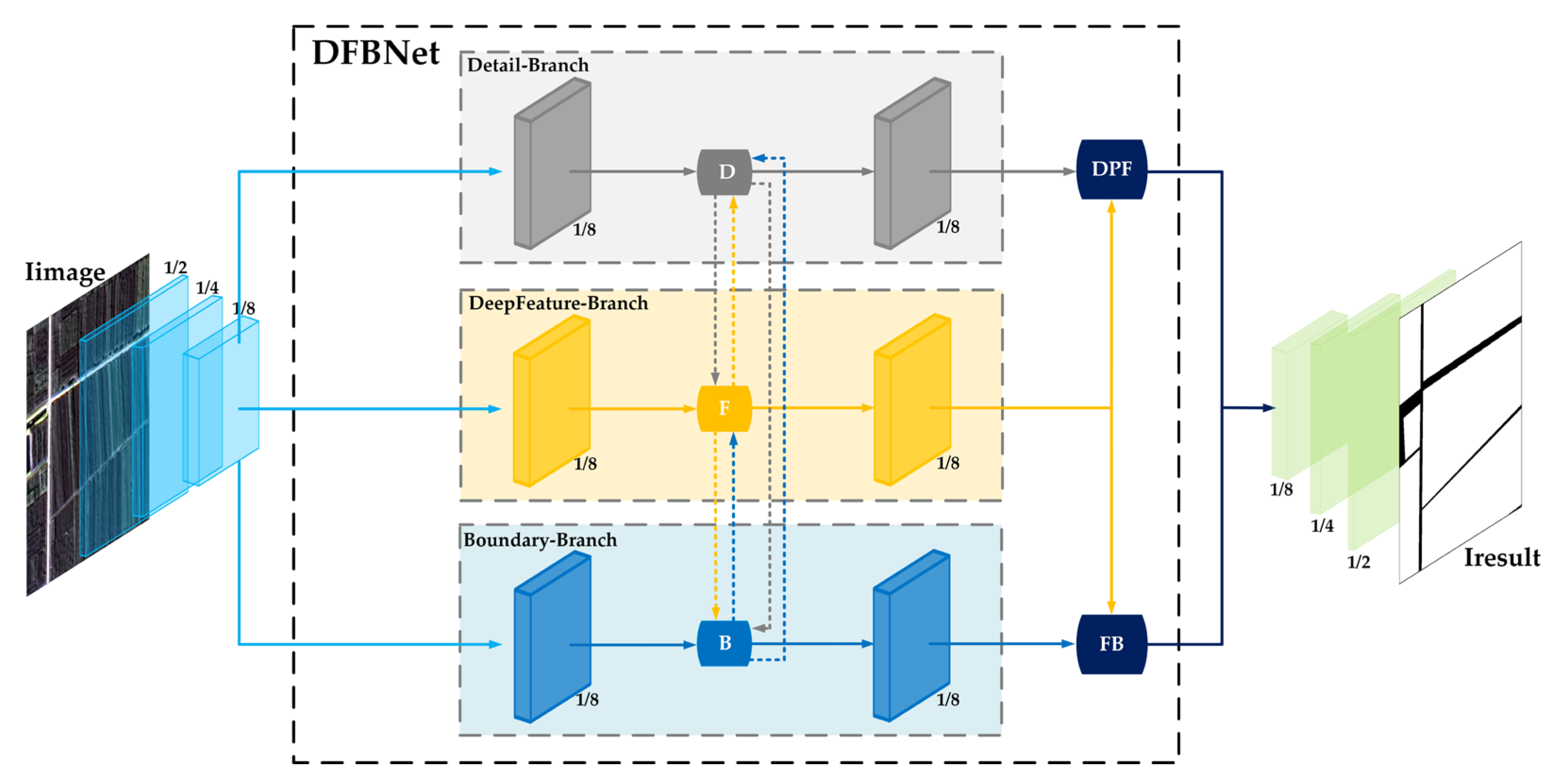
3.1. Overall Architecture of the Model

The overall structure of the DFBNet model is shown in Figure 1:

The DFBNet model is mainly divided into four parts:

• Model input part, M_input. The main function of this part is to encode the input image I_image. Through multi-step downsampling, the output FM_{preprocessing} is obtained. The purpose is to reduce the data dimension, decrease the amount of data processed by the subsequent model and the computational complexity, and provide a more appropriate data basis for the accurate judgment and processing of the subsequent model.
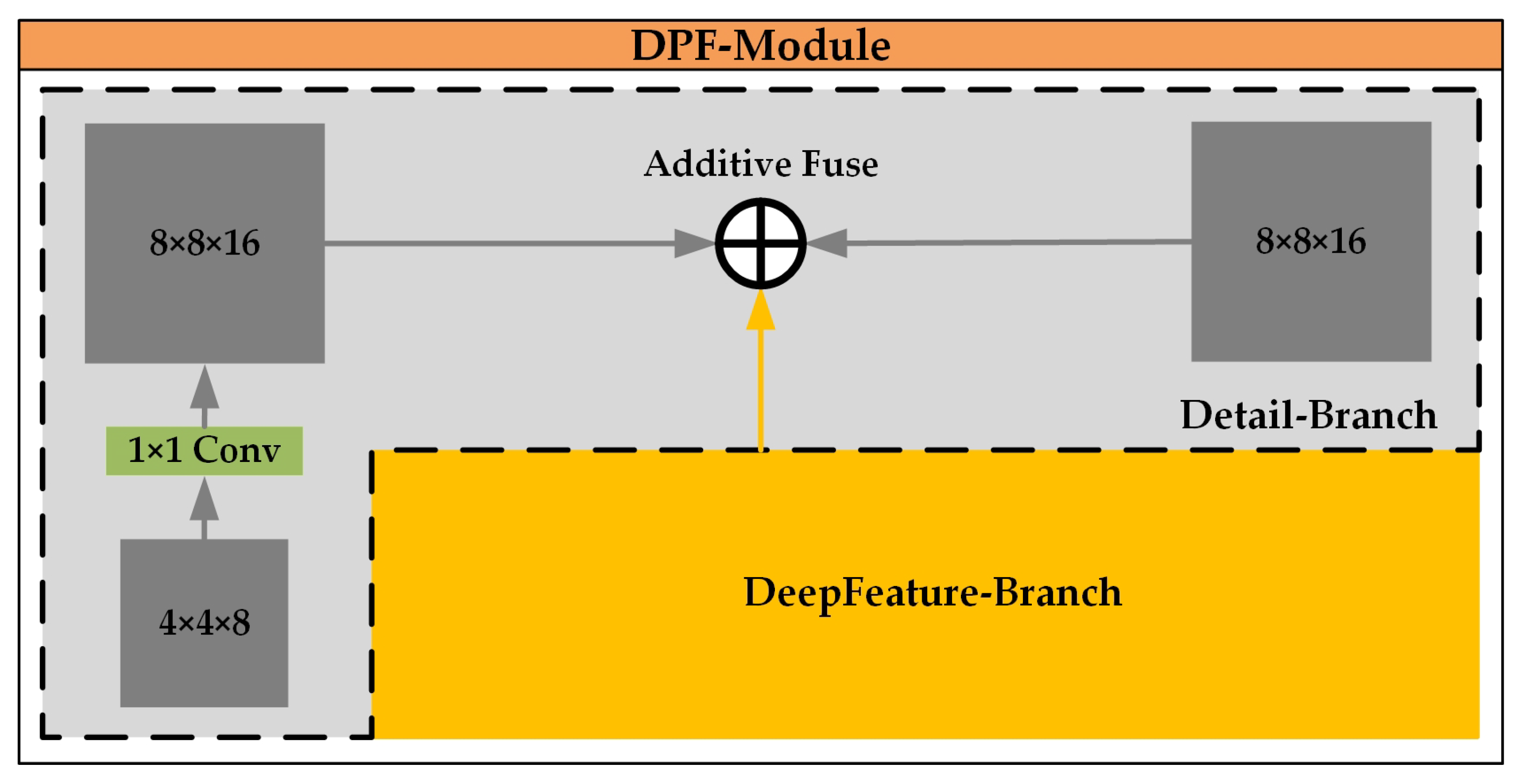
• Detail feature extraction branch, M_{Detail-Brunch}. With the model input FM_{preprocessing}, the main function of this part is to perform convolution and fusion operations on the input image block FM_{preprocessing} to extract detail features and obtain the output FM_DBR. The value of this part lies in its ability to accurately capture detail features from the preprocessed image (FM_{preprocessing}). Through convolution and fusion operations, details that are of great value for farmland identification, such as the edges and textures of furrows, are mined, and the output FM_DBR provides detailed feature data for more accurate judgment and analysis in the subsequent steps.
  Deep feature mining branch, M_{DeepFeature-Brunch}. With the model input FM_{preprocessing}, the main function of this part is to perform pooling operations on the input image block FM_{preprocessing} to mine deep features and obtain the output FM_FBR. The value of this part lies in its ability to deeply mine the deep features in the image (FM_{preprocessing}) through pooling operations, extract more representative and high-level semantic information, so that the output FM_FBR can help the subsequent model better understand the image content, and improve the processing effect of farmland image analysis.
  Boundary enhancement fusion branch, M_{Boundary-Brunch}. With the model input FM_{preprocessing}, the main function of this part is to enhance the boundary features of the input image block FM_{preprocessing} and obtain the output _FMBBR. The value of this part lies in its focus on the boundary features of the image (FM_{preprocessing}). Through enhancement processing, the boundary information in the image is highlighted, and the output FM_BBR enables the model to more clearly capture key boundary features such as farmland boundaries, which helps to improve the accuracy of the overall image analysis and related task processing in the subsequent steps.
• Model aggregation parts, M_{concatenate-DPF} and M_{concatenate-FB}. FM_DBR and FM_FBR allow information to communicate and be enhanced among different levels through M_{concatenate-DPF}, obtaining the output FM_DPFR; FM_FBR and FM_BBR mine the synergistic information among features through M_{concatenate-BF} and obtain the output FM_BFR. The value of this part lies in the fact that through specific aggregation operations (M_{concatenate-DPF} and M_{concatenate-BF}), the features extracted by different branches (such as FM_DBR, FM_FBR, and FM_BBR) can be fused and communicated with each other, the synergistic information among features can be mined, and FM_DPFR and FM_BFR can be output, respectively, providing a rich and fused feature basis for the subsequent model to output more comprehensive and relevant results.
• Model inverse encoding part, M_Inverse. The main function of this part is to inversely encode the information of FM_DPFR and FM_BFR in the model aggregation part. Through multi-step upsampling and feature adjustment, the output I_Result is obtained. The value of this part lies in inversely encoding the aggregated features (FM_DPFR and FM_BFR), using multi-step upsampling and feature adjustment operations to restore the features to an appropriate form and output I_Result, so that the model can finally output results that meet the requirements of the task and contain valid information, helping to complete the task of farmland image segmentation.

The DFBNet model integrates M_{Detail-Brunch}, M_{DeepFeature-Brunch}, and M_{Boundary-Brunch} to form a unified model M_DFBNet, and M_DFBNet can achieve the semantic segmentation of high-resolution remote-sensing images of farmland.

3.2. Model Input

The input of DFBNet is a multi-band remote-sensing image block I_image with a size of 512 × 512 × 3. It undergoes six downsampling operations. Each sampling specifically includes the following steps:

• First downsampling: Firstly, a convolution operation is performed. A set of 3 × 3 convolution kernels are used to convolve the input image I_image, and the number of convolution kernels is 3. Then, the ReLU activation function operation is carried out so that the feature map possesses nonlinear characteristics. After that, a 2 × 2 max pooling operation is conducted. This step will halve the spatial dimension of the image, resulting in an image with a size of 256 × 256 × 3.
• Second to fifth downsampling: The steps of the above downsampling are continuously repeated to gradually reduce the size of the image block. After the fifth downsampling, the spatial dimension of the image becomes 16 × 16 × 3.
• Sixth downsampling: The 3 × 3 convolution operation, the ReLU activation function operation, and the max pooling operation are carried out again. After six downsampling operations, an 8 × 8 × 3 multi-band remote-sensing image block FM_{preprocessing} is finally obtained as the output.

3.3. Model Branches

The DFBNet model is divided into the detail feature extraction branch (M_{Detail-Brunch}), the deep feature mining branch (M_{DeepFeature-Brunch}), and the boundary enhancement fusion branch (M_{Boundary-Brunch}). The detail feature extraction branch (M_{Detail-Brunch}) focuses on extracting detail features from the preprocessed image (FM_{preprocessing} after downsampling). The deep feature mining branch (M_{DeepFeature-Brunch}) can mine the deep features in the image by performing pooling operations on the input image block (FM_{preprocessing}). The boundary enhancement fusion branch (M_{Boundary-Brunch}) mainly enhances the boundary features of the input image and can highlight the boundary information in the image.

The structure of each group is as follows.

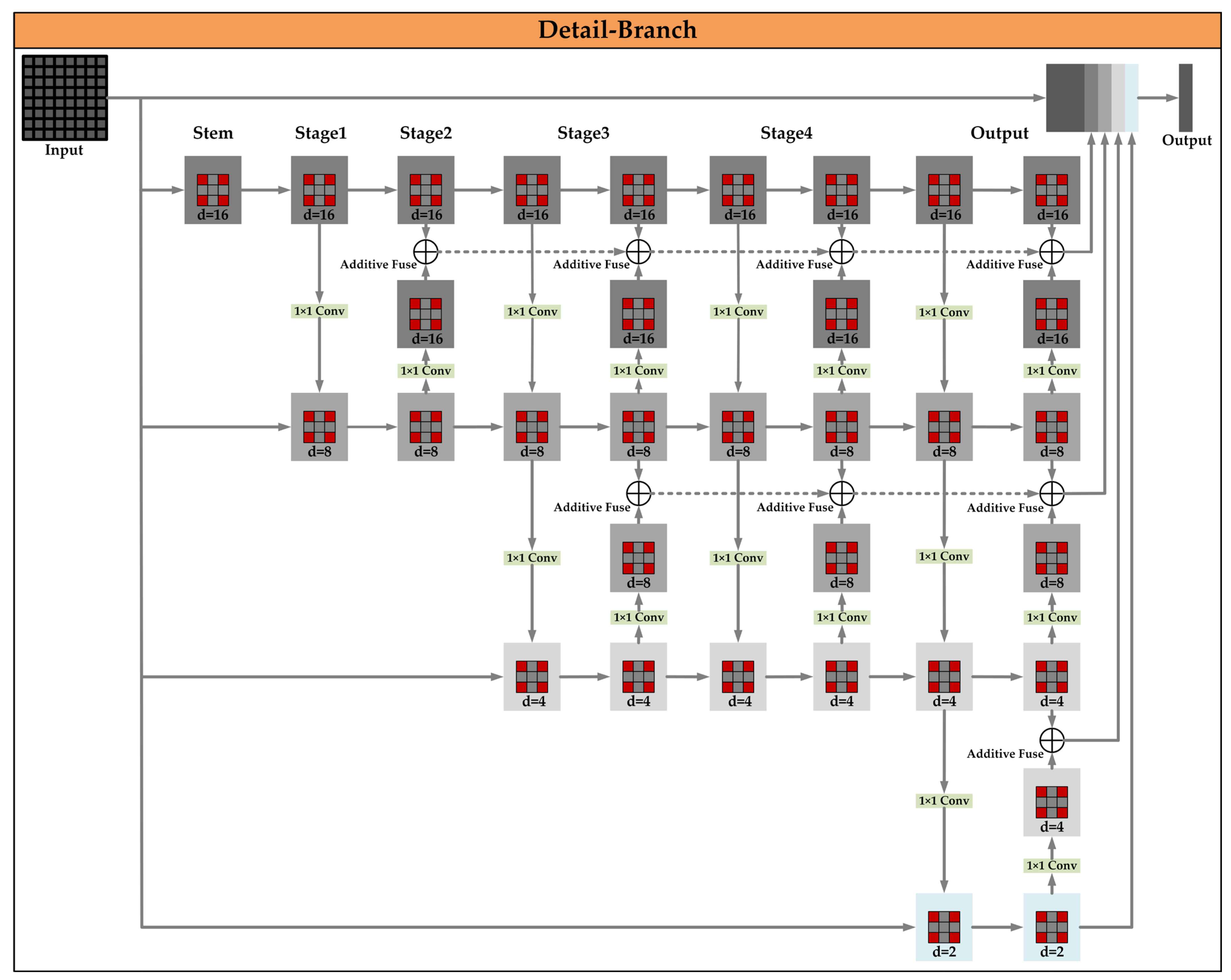
3.3.1. Detail Feature Extraction Branch

This branch mainly focuses on extracting the detail information in the image, as shown in Figure 2.

The detail feature extraction branch (M_{Detail-Brunch}) is divided into five stages: Stem, Stage 1, Stage 2, Stage 3, Stage 4, and Output.

In the Stem stage, a convolution operation is carried out using a Conv_3×3 convolution kernel with a stride of 1 and a padding of 1. This operation can keep the image size unchanged. The number of output channels is set to 16, and then a feature map I_{image-8×8×16} with a size of 8 × 8 × 16 is obtained.

Entering Stage 1, its M_Layer layer contains 2 M_bottleneck modules. In each M_bottleneck module, the 16-dimensional feature will first be reduced to 4 dimensions, and then after the Conv_3×3 convolution operation, it will be increased back to 16 dimensions. During this process, the size of the feature map I_img-8×8×16 always remains 8 × 8. In the Transition (branch generation and transition) stage, 2 branches will be generated. Among them, the first branch keeps the resolution of 8 × 8 × 16 unchanged, and the second branch performs a downsampling operation through a Conv_1×1 convolution operation with a stride of 2, halving the resolution and obtaining a feature map I_{image-4×4×8} with a size of 4 × 4 × 8.

In the M_Layer layer of Stage 2, each branch has 2 M_bottleneck modules. Each M_bottleneck contains two Conv_3×3 convolution operations to extract features. The size and dimension of the feature map I_{image-8×8×16} of the first branch remain 8 × 8 × 16, and the feature map Iimg—4 × 4 × 8 of the second branch is 4 × 4 × 8. During Fuse (feature fusion), when fusing from the second branch with a lower resolution to the first branch with a higher resolution, the number of channels of the lower resolution branch (4 × 4 × 8) will first be adjusted to 16 through a Conv_1×1 convolution layer, and then a bilinear upsampling operation will be performed to change its size to a feature map I_img-8×8×16 with a size of 8 × 8, and then it will be added and fused (Additive Fuse) with the high-resolution branch (8 × 8 × 16); for the first branch with the same resolution, no additional processing is performed.

In the M_Layer layer of Stage 3, each branch still contains 2 M_bottleneck modules. The size and dimension of the feature maps I_img-8×8×16 and I_img-4×4×8 of each branch are maintained at 8 × 8 × 16 and 4 × 4 × 8, respectively, and further feature extraction and optimization are carried out. In the Fuse (feature fusion) stage, the fusion operation in Stage 2 is repeated to ensure the information interaction and fusion between branches with different resolutions. Meanwhile, through the transition operation, a new lower resolution branch is obtained by downsampling from the second branch. The new branch has a size of 2 × 2 and the number of channels is 4, with a feature map I_img-2×2×4, and then it is fused with other branches according to similar fusion rules as in the previous steps.

In the M_Layer layer of Stage 4, there are 4 branches with sizes of I_img-8×8×16, I_img-4×4×8, I_img-2×2×4, and I_img-1×1×2, respectively. Each branch continues to perform fine feature extraction through its 2 M_bottleneck modules, and the size and dimension basically remain unchanged. During Fuse (feature fusion), the fusion operation among branches with different resolutions is fully executed again to make the features of each branch fully interact and obtain integrated multi-resolution features.

Finally, in the Output stage, the feature maps of each branch are unified to an appropriate size of 8 × 8 through upsampling and other operations, and then concatenated in the channel dimension to obtain a feature map I_img-8×8×30 with a size of 8 × 8 × (16 + 8 + 4 + 2), which is used as the final output FM_DBR.

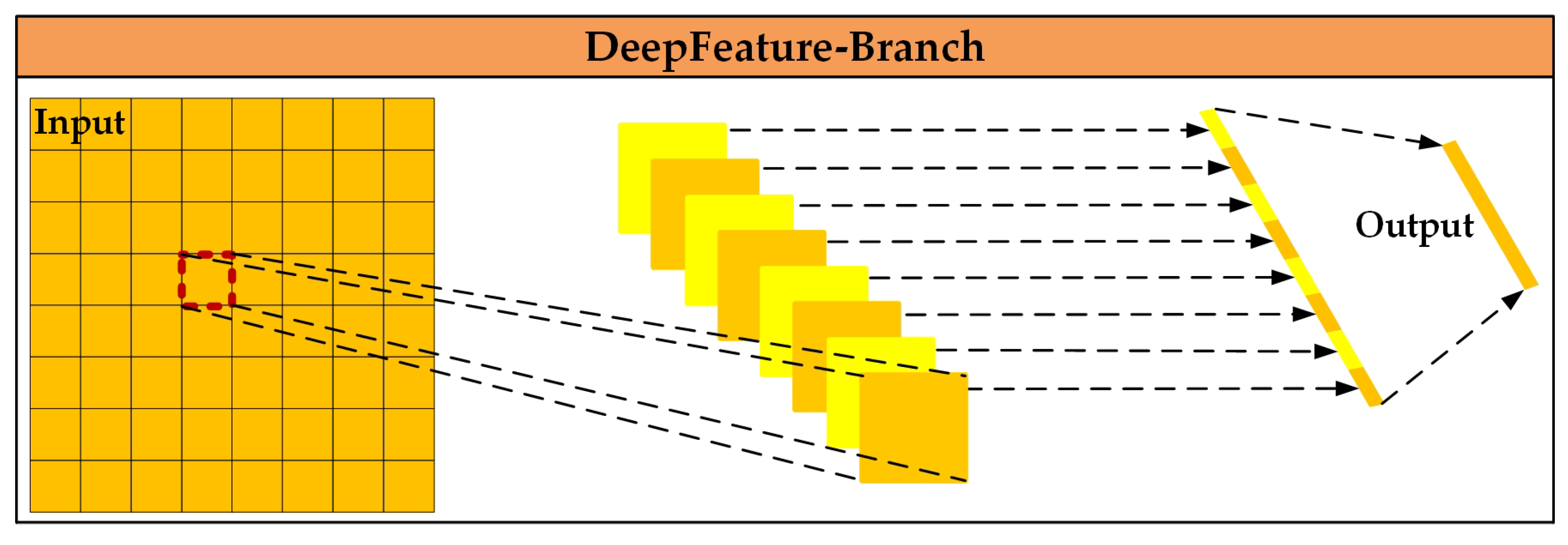
3.3.2. Deep Feature Mining Branch

This branch is dedicated to obtaining the deep semantic features of the image, as shown in Figure 3.

In the FM_FB-input layer, the 8 × 8 × 3 image FM_{preprocessing} is inputted.

In the FM_FB-operate layer, for each channel (taking one of the channels as an example), the average value of all 8 × 8 = 64 pixel values on that channel is calculated. Suppose the pixel values of the c-th channel (c = 1, 2, 3) are $x_{ij}^c$ (where i = 1, 2, …, 8, j = 1, 2, …, 8). After pooling, the calculation of the value of this channel is shown in Formula 1 as follows:

$${\displaystyle \frac{1}{8\times 8}}{\displaystyle \sum _{i=1}^8{\displaystyle \sum _{j=1}^8{x}_{ij}^c}},$$

(1)

where i = 1, 2, …, 8, j = 1, 2, …, 8, c = 1, 2, 3. By using this formula, the value of the c-th channel can be calculated. Such operations are performed on all three channels, and finally a feature vector with a length of 3 is obtained.

In the FM_FB-output layer, suppose the pixel value matrix of the first channel (the red channel) of the input image is $\left[\begin{array}{cccc}{a}_{11}& a_{12}& \cdots & a_{18}\\ a_{21}& a_{22}& \cdots & a_{28}\\ ⋮& ⋮& \ddots & ⋮\\ a_{81}& a_{82}& \cdots & a_{88}\end{array}\right]$, then the value of the red channel after pooling is ${\displaystyle \frac{1}{64}}{\displaystyle \sum _{i=1}^8{\displaystyle \sum _{j=1}^8{a}_{ij}}}$. Similarly, operations are carried out on the green channel and the blue channel, and a feature vector FM_FBR composed of three values is obtained as the output.

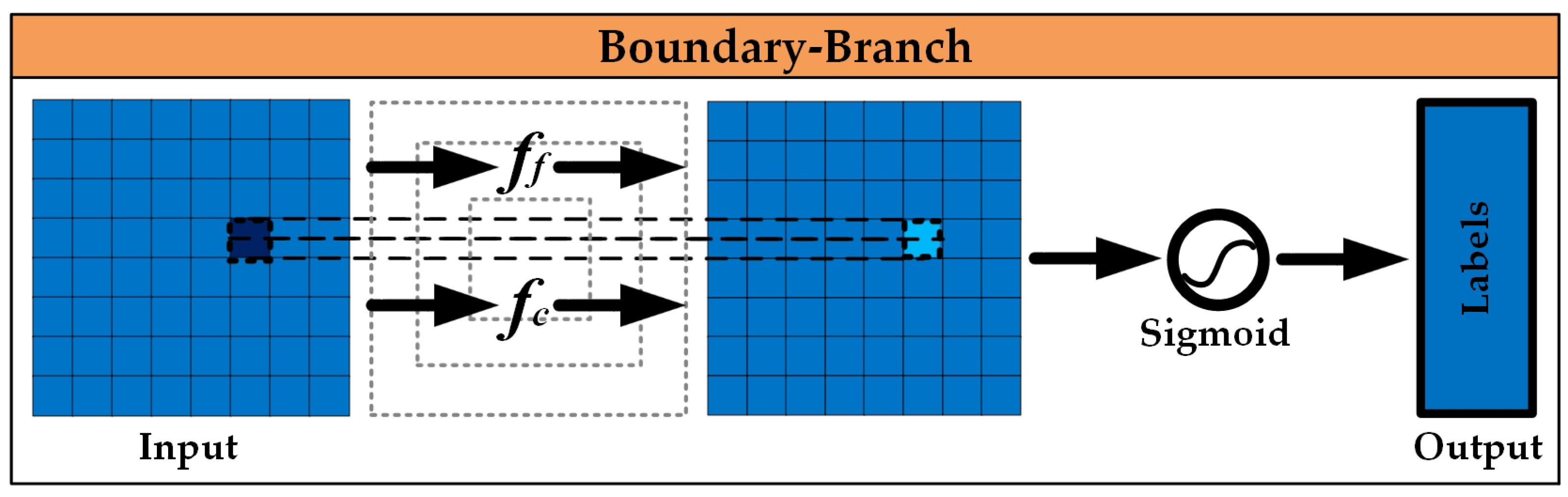
3.3.3. Boundary Enhancement Fusion Branch

This branch focuses on highlighting the boundary areas, as shown in Figure 4.

In the FM_BB-input layer, through a convolutional layer Conv_3×3 with a convolution kernel size of 3 × 3, a stride of 1, a padding of 1, and the number of output channels of 16, a feature map I_{img3-8×8×16} with a size of 8 × 8 × 16 is obtained.

Calculate f_i. For each position (x, y) (x = 1, 2, …, 8, y = 1, 2, …, 8) in the feature map I_{img3-8×8×16} with a size of 8 × 8 × 16, take the maximum value in the channel dimension. That is, for the position (x, y), its f_i value is ${max}_{c=1}^{16}$feature_{(x, y, c)}, where feature_{(x, y, c)} represents the value of the feature map I_{imge3-8×8×16} at the position (x, y) and channel c, and thus a feature map f_i with a size of 8 × 8 × 1 is obtained.

Calculate f_c. Similarly, for each position (x, y)(x = 1, 2, …, 8, y = 1, 2, …, 8) in the feature map I_{img3-8×8×16} with a size of 8 × 8 × 16, take the average value in the channel dimension. That is, for the position (x, y), its f_c value is calculated as shown in Formula 2:

$${\displaystyle \frac{1}{16}}{\displaystyle \sum _{c=1}^{16}featur{e}_{(x,y,c)}},$$

(2)

where x = 1, 2, …, 8, y = 1, 2, …, 8, c = 1. By using this formula, a feature map f_c with a size of 8 × 8 × 1 can be obtained.

Perform an addition operation on f_i and f_c to obtain a new feature map f_combined = f_i + f_c, whose size remains 8 × 8 × 1. Then, use a sigmoid activation function to compress each value in f_combined to the range between 0 and 1, obtaining the attention map I_{img-attention}.

In the FM_BB-output layer, perform an element-wise multiplication on the obtained spatial attention map I_{img-attention} and the original 8 × 8 × 16 feature map I_{img3-8×8×16} to obtain the feature map FM_BBR with enhanced boundaries as the output.

3.4. Model Information Fusion

Model information fusion aims to enrich feature information, make the features of different levels and types extracted by different branches complementary and cooperative, improve the performance of the model, enhance the feature expression ability, robustness, and generalization ability, and at the same time promote the communication and integration of information at different levels.

3.4.1. FM_DBR and FM_FBR Allow Information to Communicate and Be Enhanced Among Different Levels Through M_{concatenate-DPF}

M_{concatenate-DPF} introduces the dual-path feedback (DPF) module, which adopts a dual-path architecture; the dual-path feedback mechanism enables iterative interaction between detailed and deep features, where high-level semantic features refine fine-grained details, and low-level features guide semantic understanding, as shown in Figure 5.

Feature Adjustment: Expand the dimension of the feature vector FM_FBR output by the M_{DeepFeature-Brunch} so that it can be fused with the feature maps in the M_{Detail-Brunch}. For example, in Stage 2, convert the feature vector with a length of 16 in the M_{DeepFeature-Brunch} into a feature map I_img-8×8×16.

Fusion Operation: In the feature fusion stages from Stage 2 to Stage 4 of the M_{Detail-Brunch}, fuse the converted global feature map I_img-1×1×C with the high-resolution feature maps in the M_{Detail-Brunch}. Addition and concatenation operations can be carried out after adjusting the number of channels through 1 × 1 convolution. For example, in Stage 2, when fusing the low-resolution branch (the downsampled feature map I_img-4×4×8) with the high-resolution branch (I_img-8×8×16), simultaneously fuse the global feature map in, so that the M_{Detail-Brunch} can take global semantic information into account when extracting detail features and adjust the extraction direction of local features.

Repeat the above steps from Stage 2 to Stage 4 in the M_{Detail-Brunch} to obtain the output result FM_DPFR.

3.4.2. FM_FBR and FM_BBR Mine the Synergistic Information Among Features Through M_{concatenate-BF}

M_{concatenate-BF} introduces the bilinear fusion (BF) module, as shown in Figure 6.

Feature Preparation: The resulting feature vector FMFBR of the M_{DeepFeature-Brunch} is reshaped into a 3 × 1 matrix. The resulting feature map FM_BBR of the M_{Boundary-Brunch} is reshaped into a 16 × (8 × 8) matrix, that is, a 16 × 64 matrix. Specifically, for each channel (for a total of 16 channels), the 8 × 8 feature map is arranged in sequence by rows or columns into a vector with a length of 64, and the 16 channels then form a 16 × 64 matrix.

Operation Stage: Suppose the matrix after the M_{DeepFeature-Brunch} is reshaped as A (3 × 1), and the matrix after the M_{Boundary-Brunch} is reshaped as B (16 × 64). Calculate the bilinearly fused matrix C = A × B. According to the rules of matrix multiplication, the dimension of C is 3 × 64. Its calculation process is shown in Formula (3) as follows:

$$C_{ij}={\displaystyle \sum _{k=1}^1{A}_{ik}{B}_{kj}},$$

(3)

where i = 1, 2, 3, j = 1, 2, …, 64. By using this formula, each element value of the matrix C can be calculated.

For example, C₁₁ = A₁₁B₁₁ + A₁₂B₂₁ + A₁₃B₃₁ (here, since the range of k is 1, it is actually A₁₁B₁₁). Each element of this matrix C reflects the correlation between one dimension of the deep feature mining branch and a part of the features of the boundary enhancement fusion branch.

Output Dimension Adjustment: Perform a reshape operation on the fused 3 × 64 matrix C and convert it into a vector form. The elements in the matrix C can be read in sequence by rows or columns to obtain a vector with a length of 3 × 64 = 192, which is used as the output result FM_BFR.

3.5. Model Output

Data Preparation: Input FM_DPFR with a dimension of 8 × 8 × 30, and reshape the vector FM_BFR with a length of 192 into a feature map FM_BFR with a size of 1 × 1 × 192. Then, concatenate it with FM_DPFR with a size of 8 × 8 × 30 in the channel dimension. Obtain a new initial feature map I_Image with a dimension of 8 × 8 × (30 + 192), that is, 8 × 8 × 222.

Data Integration: Use bilinear interpolation upsampling. The goal is to gradually make the size of the feature map closer to the final desired resolution of 512 × 512. Perform the first upsampling on the 8 × 8 × 222 feature map to double its height and width, respectively, turning it into a 16 × 16 × 222 feature map. During the bilinear interpolation process, for each position where the pixel value needs to be determined in the newly generated 16 × 16 feature map (for example, the position with coordinates (x, y) where x and y are non-integer coordinates with decimal values), calculate the pixel value at this position by weighted average according to the pixels in the surrounding four original 8 × 8 feature maps (with coordinates $(⌊x⌋,⌊y⌋),(⌊x⌋,⌈y⌉),(⌈x⌉,⌊y⌋),(⌈x⌉,⌈y⌉)$, respectively) to complete the construction of the entire upsampled feature map. Use a 1 × 1 convolutional layer to adjust the number of channels of the upsampled feature map, changing the number of channels from 222 to 64. At this time, the dimension of the feature map becomes 16 × 16 × 64.

Continuously repeat the above steps of upsampling and feature adjustment to gradually expand the size of the feature map and optimize the feature representation. After six times of upsampling and feature adjustment, the output I_Result is finally obtained, with a dimension of 512 × 512 × 32.

3.6. Experimental Environment

The configuration of the experimental environment is shown in

Table 1. Experimental environment configuration.

Name	Configuration
CPU	Intel Core(TM) i7-8700K 32 G, Intel Corporation, Santa Clara, CA, USA
GPU	NVIDIA GeForce RTX 2080 Ti, NVIDIA, Santa Clara, CA, USA
Operating System	Windows 10
Deep Learning Framework	Pytorch1.12

.

• Hyperparameters: The initial learning rate was set to 0.001 and adjusted using cosine annealing. The batch size was fixed at 32. The Adam optimizer was used for training with a combination of cross-entropy and Dice loss functions to improve boundary sensitivity.
• Training Settings: All experiments were conducted on a workstation equipped with an NVIDIA GeForce RTX 2080 Ti GPU, an Intel Core i7-8700K CPU, and 32 GB of RAM. The training process ran for 100 epochs with early stopping to prevent overfitting.
• Data Preprocessing: The Hi-CNA dataset and the Netherlands Agricultural Land Dataset were resized to 512 × 512 pixels and normalized to [0, 1]. Data augmentation techniques, such as random rotation, flipping, and color jittering, were applied during training.

4. Results

4.1. Model Comparison

The primary models used for comparison in this study are UNet, DeepLabV3+, SegFormer, Mask2Former, OVSeg, and the DFBNet proposed in this paper. The UNet model, proposed in 2015, has become a benchmark for image segmentation tasks due to its simplicity and effectiveness. DeepLabV3+ (2018) and SegFormer (2021) incorporate Transformer-based architectures and advanced feature extraction methods. Mask2Former, proposed in 2022, is an image segmentation model based on Transformer, which combines masking technology, self-attention mechanism, and multi-scale feature extraction to accurately segment target objects from input images. OVSeg achieves semantic segmentation of open words by Mask-adapted CLIP. It can handle semantic segmentation of arbitrary words, breaking through the limitations of traditional methods, and has the characteristics of open words, high precision, and ease of use [18,28,29,35,36]. To ensure a thorough and reliable evaluation of the boundary segmentation algorithms, we adopt widely recognized metrics commonly used in the field. These include a combination of pixel-based error metrics, such as accuracy [35,37], pixel accuracy [38,39], IoU [40,41], and validation loss (Val Loss) [42,43]. These metrics provide a comprehensive evaluation of algorithm performance at the pixel level. The definitions for these pixel-based evaluation metrics are as follows:

$$\mathrm{Accuracy}={\displaystyle \frac{TP+TN}{TP+TN+FP+FN}},$$

(4)

$$\mathrm{Pixel} \mathrm{Accuracy}=(\mathrm{Correctly} \mathrm{Classified} \mathrm{Pixels})/(\mathrm{Total} \mathrm{Pixels}),$$

(5)

$$\mathrm{IoU}={\displaystyle \frac{TP}{TP+FP+FN}},$$

(6)

$$\mathrm{Val} \mathrm{Loss}=-{\displaystyle \sum \mathrm{y}\_\log (\mathrm{y}\_\mathrm{pred}),}$$

(7)

where y_pred is the probability distribution predicted by the model.

In addition, to address broader structural aspects, we also incorporated object-based metrics, namely over-segmentation (OS) [5,44] and under-segmentation (US) [5,45]. The object-based metrics, over-segmentation (OS) and under-segmentation (US), are defined as follows: Suppose G_i is the ground truth parcel that has the maximum intersection area with the predicted parcel P_i, where i = 1, 2, …, m, and m is the number of predicted parcels. Let area(P_i) and area(G_i) be the areas of P_i and G_i, respectively, and area(P_i∩G_i) be their overlapping area. We obtain the over-segmentation error OS(P_i) and the under-segmentation error US(G_i):

$$\mathit{OS}(G_i, P_i)=1-{\displaystyle \frac{area(P_i\cap G_i)}{area(G_i)}},$$

(8)

$$\mathit{US}(G_i, P_i)=1-{\displaystyle \frac{area(P_i\cap G_i)}{area(P_i)}}$$

(9)

When the over-segmentation (OS) metric is close to 0, it indicates that the over-segmentation error is low; when the under-segmentation (US) metric is close to 0, it indicates that the under-segmentation error is low.

4.2. Evaluation of Different Models

We initially conducted experiments using the Hi-CNA dataset, where UNet, DeepLabV3+, SegFormer, Mask2Former, OVSeg, and the DFBNet proposed in this paper were tested on the same validation set. The resulting metrics, including accuracy, pixel accuracy, IoU, and validation loss (Val Loss), are presented in

Table 2. Results of the Hi-CNA dataset.

Models	Accuracy (%)	Pixel Accuracy (%)	IoU (%)	Val Loss
UNet [35]	80.06	79.89	68.55	0.173
DeepLabV3+ [28]	81.3	81.33	69.57	0.382
SegFormer [29]	81.27	83.29	72.54	0.112
Mask2Former [18]	83.92	84.52	74.24	0.159
OVSeg [36]	82.7	82.08	71.58	0.147
DFBNet (Ours)	88.34	89.41	78.75	0.168

, along with the corresponding over-segmentation (OS) and under-segmentation (US) values.

The analysis of multiple evaluation metrics on the Hi-CNA dataset demonstrates that DFBNet performs exceptionally well. Its accuracy reaches 88.34%, showing a clear advantage over the other models. The pixel accuracy is 89.41%, reflecting outstanding performance at the pixel level. Additionally, the IoU is 78.75%, indicating a high degree of overlap between the segmented regions and the ground truth. The validation loss is 0.168, which is comparable to that of other models. Overall, DFBNet exhibits superior performance across all evaluated metrics.

In contrast, models such as UNet, DeepLabV3+, SegFormer, Mask2Former, and OVSeg exhibit shortcomings in one or more aspects, including accuracy, pixel accuracy, IoU, or validation loss. For instance, UNet shows lower accuracy and pixel accuracy, as well as a relatively low IoU. DeepLabV3+ has a higher validation loss compared to DFBNet. When comparing these metrics, DFBNet clearly demonstrates the advantages of its approach.

Next, we conducted tests on the Netherlands Agricultural Land Remote-Sensing Image Dataset. The resulting accuracy, pixel accuracy, IoU, and validation loss (Val Loss) are presented in

Table 3. Results of the Netherlands Agricultural Land Remote-Sensing Image Dataset.

Models	Accuracy (%)	Pixel Accuracy (%)	IoU (%)	Val Loss
UNet [35]	80.23	80.13	70.84	0.137
DeepLabV3+ [28]	82.8	81.79	69.62	0.479
SegFormer [29]	84.23	83.09	74.69	0.255
Mask2Former [18]	85.42	85.65	77.83	0.267
OVSeg [36]	83.62	83.9	72.89	0.249
DFBNet (Ours)	90.63	91.6	83.67	0.256

.

Similarly, on the Netherlands dataset, DFBNet excels across all evaluation metrics. Its accuracy reaches 90.63%, pixel accuracy is 91.6%, and IoU is 83.67%. These results indicate significant advantages in terms of accurate classification, pixel-level prediction, and the overall precision of the segmented regions. The validation loss is 0.256, which is moderate compared to other models. Overall, DFBNet demonstrates an excellent performance, highlighting the effectiveness of its approach.

In contrast, models such as UNet, DeepLabV3+, SegFormer, Mask2Former, and OVSeg exhibit weaknesses in one or more metrics, including accuracy, pixel accuracy, IoU, or validation loss. For example, Mask2Former and OVSeg show relatively low pixel accuracy and IoU. DeepLabV3+ suffers from poor pixel accuracy, IoU, and a higher validation loss. Although UNet has a low validation loss, its performance in other metrics is inferior to that of DFBNet, further emphasizing the advantages of the proposed method.

In the experiment of the above two datasets, we also counted the loss value of the training set of the two datasets, as shown in Figure 7.

As shown, DFBNet demonstrates faster convergence, stabilizing after approximately 50 epochs, while other models, such as UNet, exhibit oscillations in the loss value due to insufficient boundary feature learning.

Overall, DFBNet demonstrates superior performance, particularly in accuracy and Mean Intersection Over Union (IoU), aligning better with the overall classification requirements and highlighting its potential for precision agriculture applications. On two datasets with the same horizontal resolution and vertical resolution, the results of the Netherlands Agricultural Land Remote-Sensing Image Dataset were slightly better than those of the Hi-CNA dataset. This may be due to superior atmospheric conditions in the Netherlands Agricultural Land Remote-Sensing Image Dataset. Some data in the Hi-CNA dataset are affected by sunlight.

4.3. Test Results of Different Models

We randomly selected four subsets of data from the validation sets of the Hi-CNA dataset and the Netherlands Agricultural Land Remote-Sensing Image Dataset to compare the performance of the six models.

4.3.1. Test Results of the Hi-CNA Dataset

Figure 8 presents the visualization results of the test conducted on the validation sets of the six models, while Figure 9 displays the line and bar charts for the over-segmentation (OS) and under-segmentation (US) metrics based on the test results of these models.

Based on the results shown in the figures above, the following conclusions can be drawn:

Among the six models, four test images were randomly selected, and DFBNet consistently outperformed the others. Its over-segmentation (OS) values were 0.021, 0.119, 0.055, and 0.069, while its under-segmentation (US) values were 0.207, 0.190, 0.091, and 0.090, all of which were the lowest across the models. This demonstrates that DFBNet effectively controlled both over-segmentation and under-segmentation. In contrast, UNet, DeepLabV3+, SegFormer, Mask2Former, and OVSeg exhibited varying degrees of over-segmentation or under-segmentation, with overall segmentation performance falling short compared to DFBNet.

4.3.2. Test Results of the Netherlands Agricultural Land Remote-Sensing Image Dataset

Figure 10 presents the visualization results from the tests conducted on the validation sets of the six models, while Figure 11 displays the line and bar charts for the over-segmentation (OS) and under-segmentation (US) metrics based on the test results of these models.

Based on the results illustrated in the figures, the following conclusions can be drawn:

Among the six models, DFBNet demonstrates the best performance. Its over-segmentation (OS) values are 0.017, 0.047, 0.040, and 0.061, and its under-segmentation (US) values are 0.032, 0.067, 0.105, and 0.061, all of which are the lowest across the models. This indicates that DFBNet achieves superior control over both over-segmentation and under-segmentation, demonstrating high segmentation accuracy. In comparison, UNet, DeepLabV3+, SegFormer, Mask2Former, and OVSeg exhibit varying degrees of over-segmentation and under-segmentation, resulting in an overall segmentation performance that falls short of DFBNet.

4.4. Ablation Experiment

4.4.1. Determine the Ablation Objects

The ablation experiment focuses on the dual-path feedback (DPF) module and bilinear fusion (BF) module. Specifically, we conducted experiments by altering the fusion mechanism within the DPF module (DFBNet-DPF). This involved modifying the information transmission pathway between the Detail-Branch and the Deep Feature-Branch and removing the parallel structure to evaluate its impact on model performance.

To evaluate the effectiveness of the BF module in the DFBNet, we conducted an ablation study by comparing the performance of the complete model with versions that omit the BF module (DFBNet-BF).

4.4.2. Ablation Experimental Setup

Training Process: The ablation experiments utilized the Hi-CNA dataset and the Netherlands Agricultural Land Remote-Sensing Image Dataset, ensuring consistency in training parameters across all experiments. For the ablation study of the DPF module, the model was retrained after implementing the modifications to the relevant mechanisms. For the ablation experiment of BF module, we removed the BF module to assess the impact of this fusion method on segmentation performance. Without the BF module, the model relies solely on the traditional feature extraction and fusion mechanisms.

Evaluation Metrics: The performance of the ablation experiments was assessed using metrics such as over-segmentation (OS) and under-segmentation (US), comparing the results with those of the complete DPF module and BF module on the validation sets.

4.4.3. Result Analysis

As shown in

Table 4. Precision comparison between different models on two datasets in ablation experiments.

Datasets	Models	Accuracy (%)	Pixel Accuracy (%)	IoU (%)	Val Loss
The Hi-CNA Dataset	DFBNet	88.34	89.41	78.75	0.168
	DFBNet-DPF	86.50	84.73	72.14	0.184
	DFBNet-BF	87.05	85.10	73.25	0.175
The Netherlands Agricultural Land Remote-Sensing Image Dataset	DFBNet	90.63	91.6	83.67	0.256
	DFBNet-DPF	89.15	87.10	75.83	0.269
	DFBNet-BF	89.40	87.35	76.42	0.262

, the ablation experiments demonstrate that removing either the DPF or BF module results in a significant drop in segmentation performance, with the absence of the DPF module causing a more pronounced impact on metrics such as IoU and validation loss, highlighting the critical role of both modules in the effectiveness of DFBNet.

Figure 12 illustrates the visualization results before and after the ablation experiment on the Hi-CNA dataset, while Figure 13 presents the line and bar charts for the over-segmentation (OS) and under-segmentation (US) metrics, comparing the results before and after the experiment.

Figure 14 presents the visualization results of the comparison before and after the ablation experiment on the Netherlands Agricultural Land Remote-Sensing Image Dataset. Figure 15 displays the line and bar charts for the over-segmentation (OS) and under-segmentation (US) metrics, illustrating the comparison results before and after the ablation experiment.

Ablation Results for the DPF Module: The results from both the Hi-CNA dataset and the Netherlands Agricultural Land Remote-Sensing Image Dataset demonstrate a decline in performance when the information transmission mechanism between the Detail-Branch and the Deep Feature-Branch is altered. This finding underscores the importance of the original information transmission design within the DPF module, which is essential for effectively integrating features and enhancing segmentation accuracy.

Ablation Results for the BF Module: The results from the Hi-CNA dataset and the Netherlands Agricultural Land Remote-Sensing Image Dataset are shown in the figure above, demonstrate that the bilinear fusion (BF) module significantly improves segmentation accuracy, particularly in challenging cases where fine-grained details and complex boundaries are crucial for precise crop delineation.

4.5. Statistical Significance Testing

To further validate that the performance improvements achieved by DFBNet in farmland boundary segmentation are statistically significant, we conducted multiple independent experiments on two datasets: the Hi-CNA dataset and the Netherlands Agricultural Land Remote-Sensing Image Dataset. For each dataset, we measured key metrics (accuracy, pixel accuracy, IoU, and Val Loss) and applied Student’s t-test for continuous metrics.

4.5.1. Experimental Setup

Experiments were performed on the Hi-CNA dataset and the Netherlands Agricultural Land Remote-Sensing Image Dataset under consistent hardware conditions (NVIDIA GeForce RTX 2080 Ti GPU). For each model, 10 independent runs were conducted using randomly partitioned training sets.

Table 5. Performance on the Hi-CNA dataset and the Netherlands Agricultural Land Remote-Sensing Image Dataset (training set, 10 runs, Mean ± SD).

Datasets	Models	Accuracy (%)	Pixel Accuracy (%)	IoU (%)
The Hi-CNA Dataset	UNet [35]	80.06 ± 0.50	79.89 ± 0.60	68.55 ± 0.80
	DeepLabV3+ [28]	81.30 ± 0.55	81.33 ± 0.65	69.57 ± 0.75
	SegFormer [29]	81.27 ± 0.60	83.29 ± 0.70	72.54 ± 0.80
	Mask2Former [18]	83.92 ± 0.65	84.52 ± 0.70	74.24 ± 0.85
	OVSeg [36]	82.70 ± 0.60	82.08 ± 0.65	71.58 ± 0.80
	DFBNet (Ours)	88.34 ± 0.70	89.41 ± 0.75	78.75 ± 0.85
The Netherlands Agricultural Land Remote-Sensing Image Dataset	UNet [35]	80.23 ± 0.55	80.13 ± 0.60	70.84 ± 0.80
	DeepLabV3+ [28]	82.80 ± 0.58	81.79 ± 0.63	69.62 ± 0.75
	SegFormer [29]	84.23 ± 0.65	83.09 ± 0.70	74.69 ± 0.85
	Mask2Former [18]	85.42 ± 0.62	85.65 ± 0.70	77.83 ± 0.90
	OVSeg [36]	83.62 ± 0.60	83.90 ± 0.65	72.89 ± 0.85
	DFBNet (Ours)	90.63 ± 0.50	91.60 ± 0.55	83.67 ± 0.80

shows the average performance (mean ± standard deviation) observed on the training data:

4.5.2. Student’s t-Test Analysis

For continuous metrics (accuracy, pixel accuracy, and IoU), we employed Student’s t-test to compare the mean performance of DFBNet with that of each baseline model. We set the significance level at p < 0.05.

Table 6. p-values from Student’s t-test Comparing DFBNet with baseline models.

Datasets	Compared Models	Accuracy p-Value	Pixel Accuracy p-Value	IoU p-Value
The Hi-CNA Dataset	UNet [35]	0.001	0.001	0.002
	DeepLabV3+ [28]	0.001	0.001	0.001
	SegFormer [29]	0.001	0.000	0.001
	Mask2Former [18]	0.002	0.001	0.002
	OVSeg [36]	0.001	0.001	0.001
The Netherlands Agricultural Land Remote-Sensing Image Dataset	UNet [35]	0.001	0.001	0.001
	DeepLabV3+ [28]	0.001	0.001	0.001
	SegFormer [29]	0.002	0.001	0.001
	Mask2Former [18]	0.002	0.001	0.002
	OVSeg [36]	0.001	0.001	0.001

presents the resulting p-values from these comparisons:

As shown in Table 6, the improvements in accuracy, pixel accuracy, and IoU achieved by DFBNet over each of the baseline models are statistically significant (p < 0.05).

4.5.3. Discussion

The statistical significance tests provide robust evidence that the performance gains achieved by DFBNet are not attributable to random variation. The Student’s t-test demonstrated that DFBNet significantly outperforms UNet, DeepLabV3+, SegFormer, Mask2Former, and OVSeg in terms of accuracy, pixel accuracy, and IoU on both the Hi-CNA dataset and the Netherlands Agricultural Land Dataset. These findings validate our claim that the novel three-branch architecture of DFBNet—which simultaneously captures fine details, global semantic information, and reinforced boundary features—is better suited to address the challenges of farmland boundary segmentation.

Future work will extend these analyses to even larger and more diverse datasets and explore additional statistical methods to further confirm the robustness and generalizability of DFBNet across various real-world scenarios.

5. Discussion

5.1. Summary of Research Results

This study proposed the Detail and Deep Feature Multi-Branch Fusion Network for High-Resolution Farmland Remote-Sensing Segmentation (DFBNet), achieving a series of significant and meaningful results:

• Segmentation Accuracy: Experimental results demonstrate that DFBNet excels in the segmentation accuracy of farmland boundaries. It effectively identifies farmland areas and accurately segments their boundaries. Compared with traditional methods and existing deep learning models, DFBNet shows clear advantages in segmentation accuracy-related metrics, such as accuracy, pixel accuracy, and IoU. The structural design of DFBNet enables it to capture complex farmland features and boundary details, refining segmentation from small-area plots to entire farmland boundaries, meeting the requirements for precise boundary delineation.
• Anti-Interference Capability: When faced with complex background interference in remote-sensing images, such as shadows, weeds, and differences in farmland morphology, DFBNet exhibits strong anti-interference capability. Its dual-branch feature learning and progressive boundary refinement processes allow the model to distinguish essential features of farmland from interference factors. As a result, it reliably identifies farmland areas even in challenging environments, providing accurate boundary information. This robustness offers significant technical support for monitoring farmland boundaries in practical agricultural production.

5.2. Comparison with Existing Methods

• Traditional Image Processing Methods: Traditional image processing methods, such as UNet and SegFormer, have notable limitations in farmland boundary segmentation. These methods are highly sensitive to illumination conditions, noise, and the complex structures of farmland areas. For instance, under uneven illumination, threshold-based methods struggle to determine appropriate thresholds, leading to inaccurate and fragmented segmentation results. In contrast, DFBNet, with its deep learning architecture, can automatically learn features of small-area plots and boundary information. This ensures greater robustness to illumination variations and noise.
• General Deep Learning Models: Although general deep learning models have achieved some success in image segmentation, they often face challenges in segmenting farmland boundaries. Issues such as occlusion, overlapping, and complex backgrounds in small-area farmland plots reduce their effectiveness. For example, methods such as UNet and DeepLabV3+ fail to fully capture subtle features and intricate structures, resulting in inaccurate boundary delineation. In contrast, DFBNet overcomes these challenges through its innovative architecture, which includes the detail feature extraction branch (Detail-Branch), deep feature mining branch (Deep Feature-Branch), and boundary enhancement fusion branch (Boundary-Branch). The Detail-Branch focuses on extracting fine-grained information from images, the Deep Feature-Branch specializes in obtaining high-level semantic features, and the Boundary-Branch emphasizes boundary enhancement. Combined with the dual-path feedback and bilinear fusion structures, these components progressively refine boundary segmentation, improving the model’s ability to handle complex farmland features effectively.

5.3. Computational Efficiency

The computational efficiency of DFBNet was assessed to evaluate its practicality in real-world applications. On an NVIDIA GeForce RTX 2080 Ti GPU, the model processed a single 512 × 512 image in approximately 120 ms, demonstrating near-real-time processing capabilities. The peak GPU memory usage during segmentation tasks was 8.1 GB, which aligns with the requirements of typical high-performance systems. In addition to runtime and memory usage, we also calculated the FLOPs (floating-point operations per second) and the number of parameters for DFBNet to provide a more detailed perspective on its computational complexity. FLOPs and parameters are essential factors in understanding a model’s efficiency, as they directly impact the computational resources needed during both training and inference. DFBNet, with 100 GFLOPs and 35 million parameters, is optimized to balance segmentation accuracy with computational demand.

For comparison, the runtime and memory usage of baseline models are summarized in

Table 7. Computational efficiency of different models.

Models	Average Runtime (ms)	Peak Memory Usage (GB)	FLOPs (GFLOPs)	Parameters (M)
UNet [35]	80	5.2	45	31
DeepLabV3+ [28]	180	8.3	160	64
SegFormer [29]	200	9.0	70	40
Mask2Former [18]	190	9.7	220	90
OVSeg [36]	160	7.5	180	66
DFBNet (Ours)	120	8.1	100	35

. While models such as UNet exhibit slightly lower memory usage, DFBNet balances computational demands with its superior segmentation accuracy. Notably, DFBNet balances computational demands with its superior segmentation accuracy, offering efficient performance even with higher complexity models such as DeepLabV3+ (160 GFLOPs, 64 M parameters) and Mask2Former (220 GFLOPs, 90 M parameters).

Future work will explore optimization strategies to enhance the deployment efficiency of DFBNet, including techniques such as model pruning, quantization, and lightweight architecture integration, all of which can further reduce both the FLOPs and memory usage while maintaining or improving segmentation performance.

5.4. Limitations and Future Work

While DFBNet demonstrates strong performance in high-resolution farmland remote-sensing segmentation, there are several limitations that need to be addressed to further enhance its capabilities. Below, we discuss the key limitations of the model and outline directions for future work.

• Performance on Unseen Farmland Types: DFBNet performs well on the datasets it was trained on, such as the Hi-CNA dataset and the Netherlands Agricultural Land dataset, but it faces challenges when applied to unseen farmland areas with different crop types, terrain, and environmental conditions. The model may struggle in regions with unfamiliar crops or geographic features.
• Pixel-Level Crop Classification: DFBNet is effective at segmenting farmland boundaries but does not perform pixel-level crop classification. This limitation is especially noticeable when distinguishing between crops with similar spectral properties (e.g., wheat and barley). This could lead to inaccuracies in crop distribution prediction.
• Impact of Different Crop Types: The segmentation accuracy can be affected by the presence of different crop types, particularly those with similar spectral characteristics or crops at different growth stages. This can complicate the segmentation task, especially when crops are grown close together.

To address the limitations outlined above and further enhance DFBNet’s performance, future work will focus on the following areas:

• Enhancing Generalization to Unseen Farmland Types: We will explore domain adaptation techniques—for example, using self-supervised feature learning and clustering-based methods in an unsupervised framework, and employing consistency regularization and pseudo-labeling in a semi-supervised setup. These approaches pose challenges such as ensuring pseudo-label quality and handling unlabeled data variability. Additionally, transfer learning will be used to fine-tune the model on new, diverse agricultural datasets, though domain shifts may require advanced alignment strategies.
• Integrating Pixel-Level Crop Classification: Future versions of DFBNet will incorporate pixel-level crop classification alongside segmentation tasks. This could be achieved by combining segmentation and pixel-wise classification in a unified framework. Multi-source data such as vegetation indices will also be integrated to enhance the model’s ability to distinguish between similar crop types.
• Improving Handling of Crop Diversity: To address the impact of different crop types, we will explore multi-scale feature extraction and integrate time-series remote-sensing data. These additions will help the model to better manage crops at different growth stages and sizes, improving segmentation accuracy in diverse agricultural settings.

By focusing on these future directions, we aim to enhance DFBNet’s generalization, crop classification capabilities and handling of diverse crop types, further solidifying its role as a robust tool for high-resolution farmland segmentation in precision agriculture and remote sensing.

6. Conclusions

The DFBNet model proposed in this paper offers an innovative and effective solution for the semantic segmentation of farmland remote-sensing images.

The DFBNet model addresses the challenges faced by traditional methods in the remote-sensing monitoring of crops, particularly the loss of boundary characteristics and small-area plot details when extracting deep features. Through its unique three-branch architecture—comprising the detail feature extraction branch, the deep feature mining branch, and the boundary enhancement fusion branch—the model successfully overcomes these limitations. The design of the multi-branch fusion mechanism is central to the model’s innovation, enabling simultaneous processing of image information from multiple perspectives. Specifically, the detail feature extraction branch captures fine-grained local details, the deep feature mining branch extracts high-level semantic features, and the boundary enhancement fusion branch emphasizes the retention and enhancement of boundary information. These branches work in tandem, complementing each other to achieve comprehensive and precise feature extraction for farmland remote-sensing images.

The DFBNet model demonstrates significant value in practice. The experimental results show that it outperforms five traditional methods in terms of overall accuracy and boundary semantic segmentation effectiveness. On both the Hi-CNA dataset and the Netherlands Agricultural Land Remote-Sensing Image Dataset, the model achieved excellent performance across key metrics, including accuracy, pixel accuracy, and IoU. This superior performance indicates that DFBNet can accurately delineate farmland boundaries, providing critical data for agricultural yield estimation and precision farming decision-making. By delivering precise farmland boundary segmentation and plot identification, the model enables more accurate crop yield predictions and farmland quality assessments. This, in turn, supports the development of scientific and well-informed strategies for precision agriculture, facilitating a shift toward more refined and intelligent agricultural management.

The broad application prospects and practical value of DFBNet highlight its potential to advance the agricultural sector by promoting efficiency, sustainability, and innovation. The following are the specific application scenarios:

• Precision Agriculture Management: Through high-precision farmland segmentation, DFBNet can help farmers to achieve precise fertilization, precision irrigation, and other agricultural management means, thereby reducing resource waste and improving agricultural production efficiency.
• Crop Yield Forecast: By accurately classifying crop areas, DFBNet can provide more accurate crop yield prediction to support agricultural production planning and decision-making.
• Farmland Monitoring and Disaster Warning: The model can be used to monitor the growth state of the farmland, and find the problems such as pests and diseases and drought in time, so as to improve the emergency response ability of agricultural production.
• Multi-Source Remote-Sensing Data Fusion: DFBNet can also be combined with other remote-sensing data (e.g., radar, LIDAR) to provide more accurate field plot division and crop monitoring.

Through these applications, DFBNet can not only support the precision management of agriculture, but also play an important role in agricultural resource scheduling, crop disaster monitoring, and so on.

References

1. Ma, Z.; Li, W.; Warner, T.A.; He, C.; Wang, X.; Zhang, Y.; Guo, C.; Cheng, T.; Zhu, Y.; Cao, W. A framework combined stacking ensemble algorithm to classify crop in complex agricultural landscape of high altitude regions with Gaofen-6 imagery and elevation data. Int. J. Appl. Earth Obs. Geoinf. 2023, 122, 103386. [Google Scholar] [CrossRef]
2. Yeom, J.-M.; Jeong, S.; Deo, R.C.; Ko, J. Mapping rice area and yield in northeastern Asia by incorporating a crop model with dense vegetation index profiles from a geostationary satellite. GIScience Remote Sens. 2021, 58, 1–27. [Google Scholar] [CrossRef]
3. Chen, W.; Liu, G. A novel method for identifying crops in parcels constrained by environmental factors through the integration of a Gaofen-2 high-resolution remote sensing image and Sentinel-2 time series. IEEE J. Sel. Top. Appl. Earth Obs. Remote Sens. 2023, 17, 450–463. [Google Scholar] [CrossRef]
4. Jo, H.-W.; Park, E.; Sitokonstantinou, V.; Kim, J.; Lee, S.; Koukos, A.; Lee, W.-K. Recurrent U-Net based dynamic paddy rice mapping in South Korea with enhanced data compatibility to support agricultural decision making. GIScience Remote Sens. 2023, 60, 2206539. [Google Scholar] [CrossRef]
5. Awad, B.; Erer, I. FAUNet: Frequency Attention U-Net for Parcel Boundary Delineation in Satellite Images. Remote Sens. 2023, 15, 5123. [Google Scholar] [CrossRef]
6. Yang, M.-D.; Huang, K.-S.; Kuo, Y.-H.; Tsai, H.P.; Lin, L.-M. Spatial and spectral hybrid image classification for rice lodging assessment through UAV imagery. Remote Sens. 2017, 9, 583. [Google Scholar] [CrossRef]
7. Liu, W.; Dong, J.; Xiang, K.; Wang, S.; Han, W.; Yuan, W. A sub-pixel method for estimating planting fraction of paddy rice in Northeast China. Remote Sens. Environ. 2018, 205, 305–314. [Google Scholar] [CrossRef]
8. Matton, N.; Sepulcre Canto, G.; Waldner, F.; Valero, S.; Morin, D.; Inglada, J.; Arias, M.; Bontemps, S.; Koetz, B.; Defourny, P. An automated method for annual cropland mapping along the season for various globally-distributed agrosystems using high spatial and temporal resolution time series. Remote Sens. 2015, 7, 13208–13232. [Google Scholar] [CrossRef]
9. Yang, L.; Wang, L.; Abubakar, G.A.; Huang, J. High-resolution rice mapping based on SNIC segmentation and multi-source remote sensing images. Remote Sens. 2021, 13, 1148. [Google Scholar] [CrossRef]
10. Yang, Y.; Huang, Q.; Wu, W.; Luo, J.; Gao, L.; Dong, W.; Wu, T.; Hu, X. Geo-parcel based crop identification by integrating high spatial-temporal resolution imagery from multi-source satellite data. Remote Sens. 2017, 9, 1298. [Google Scholar] [CrossRef]
11. Valero, S.; Morin, D.; Inglada, J.; Sepulcre, G.; Arias, M.; Hagolle, O.; Dedieu, G.; Bontemps, S.; Defourny, P.; Koetz, B. Production of a dynamic cropland mask by processing remote sensing image series at high temporal and spatial resolutions. Remote Sens. 2016, 8, 55. [Google Scholar] [CrossRef]
12. Rydberg, A.; Borgefors, G. Integrated method for boundary delineation of agricultural fields in multispectral satellite images. IEEE Trans. Geosci. Remote Sens. 2001, 39, 2514–2520. [Google Scholar] [CrossRef]
13. Yu, J.; Tan, J.; Wang, Y. Ultrasound speckle reduction by a SUSAN-controlled anisotropic diffusion method. Pattern Recognit. 2010, 43, 3083–3092. [Google Scholar] [CrossRef]
14. Fetai, B.; Oštir, K.; Kosmatin Fras, M.; Lisec, A. Extraction of visible boundaries for cadastral mapping based on UAV imagery. Remote Sens. 2019, 11, 1510. [Google Scholar] [CrossRef]
15. Wu, C.; Zhang, L.; Du, B.; Chen, H.; Wang, J.; Zhong, H. UNet-Like Remote Sensing Change Detection: A review of current models and research directions. IEEE Geosci. Remote Sens. Mag. 2024, 12, 305–334. [Google Scholar] [CrossRef]
16. Fu, B.; He, X.; Yao, H.; Liang, Y.; Deng, T.; He, H.; Fan, D.; Lan, G.; He, W. Comparison of RFE-DL and stacking ensemble learning algorithms for classifying mangrove species on UAV multispectral images. Int. J. Appl. Earth Obs. Geoinf. 2022, 112, 102890. [Google Scholar] [CrossRef]
17. Zhan, Z.; Xiong, Z.; Huang, X.; Yang, C.; Liu, Y.; Wang, X. Multi-Scale Feature Reconstruction and Inter-Class Attention Weighting for Land Cover Classification. IEEE J. Sel. Top. Appl. Earth Obs. Remote Sens. 2023, 17, 1921–1937. [Google Scholar] [CrossRef]
18. Cheng, B.; Misra, I.; Schwing, A.G.; Kirillov, A.; Girdhar, R. Masked-attention mask transformer for universal image segmentation. In Proceedings of the IEEE/CVF Conference on Computer Vision and Pattern Recognition, New Orleans, LA, USA, 18–24 June 2022; pp. 1290–1299. [Google Scholar]
19. Lu, Y.; James, T.; Schillaci, C.; Lipani, A. Snow detection in alpine regions with Convolutional Neural Networks: Discriminating snow from cold clouds and water body. GIScience Remote Sens. 2022, 59, 1321–1343. [Google Scholar] [CrossRef]
20. Qi, L.; Zuo, D.; Wang, Y.; Tao, Y.; Tang, R.; Shi, J.; Gong, J.; Li, B. Convolutional Neural Network-Based Method for Agriculture Plot Segmentation in Remote Sensing Images. Remote Sens. 2024, 16, 346. [Google Scholar] [CrossRef]
21. Xu, Z.; Zhang, W.; Zhang, T.; Li, J. HRCNet: High-resolution context extraction network for semantic segmentation of remote sensing images. Remote Sens. 2020, 13, 71. [Google Scholar] [CrossRef]
22. Xu, Y.; Jiang, J. High-resolution boundary-constrained and context-enhanced network for remote sensing image segmentation. Remote Sens. 2022, 14, 1859. [Google Scholar] [CrossRef]
23. Gonçalves, D.N.; Marcato, J., Jr.; Carrilho, A.C.; Acosta, P.R.; Ramos, A.P.M.; Gomes, F.D.G.; Osco, L.P.; Oliveira, M.D.; Martins, J.A.C.; Damasceno, G.A., Jr.; et al. Transformers for mapping burned areas in Brazilian Pantanal and Amazon with PlanetScope imagery. Int. J. Appl. Earth Obs. Geoinf. 2023, 116, 103151. [Google Scholar] [CrossRef]
24. Lu, T.Y.; Gao, M.X.; Wang, L. Crop classification in high-resolution remote sensing images based on multi-scale feature fusion semantic segmentation model. Front. Plant Sci. 2023, 14, 1196634. [Google Scholar] [CrossRef] [PubMed]
25. Zhang, J.; Xu, S.; Sun, J.; Ou, D.; Wu, X.; Wang, M. Unsupervised adversarial domain adaptation for agricultural land extraction of remote sensing images. Remote Sens. 2022, 14, 6298. [Google Scholar] [CrossRef]
26. Ma, X.; Wu, Q.; Zhao, X.; Zhang, X.; Pun, M.-O.; Huang, B. Sam-assisted remote sensing imagery semantic segmentation with object and boundary constraints. IEEE Trans. Geosci. Remote Sens. 2024, 62, 5636916. [Google Scholar] [CrossRef]
27. Ma, L.; Liu, Y.; Zhang, X.; Ye, Y.; Yin, G.; Johnson, B.A. Deep learning in remote sensing applications: A meta-analysis and review. ISPRS J. Photogramm. Remote Sens. 2019, 152, 166–177. [Google Scholar] [CrossRef]
28. Chen, L.-C.; Zhu, Y.; Papandreou, G.; Schroff, F.; Adam, H. Encoder-decoder with atrous separable convolution for semantic image segmentation. In Proceedings of the European Conference on Computer Vision (ECCV), Munich, Germany, 8–14 September 2018; pp. 801–818. [Google Scholar]
29. Xie, E.; Wang, W.; Yu, Z.; Anandkumar, A.; Alvarez, J.M.; Luo, P. SegFormer: Simple and efficient design for semantic segmentation with transformers. Adv. Neural Inf. Process. Syst. 2021, 34, 12077–12090. [Google Scholar]
30. Li, J.; Pei, Y.; Zhao, S.; Xiao, R.; Sang, X.; Zhang, C. A review of remote sensing for environmental monitoring in China. Remote Sens. 2020, 12, 1130. [Google Scholar] [CrossRef]
31. Waldner, F.; Diakogiannis, F.I. Deep learning on edge: Extracting field boundaries from satellite images with a convolutional neural network. Remote Sens. Environ. 2020, 245, 111741. [Google Scholar] [CrossRef]
32. Sun, Z.; Zhong, Y.; Wang, X.; Zhang, L. Identifying cropland non-agriculturalization with high representational consistency from bi-temporal high-resolution remote sensing images: From benchmark datasets to real-world application. ISPRS J. Photogramm. Remote Sens. 2024, 212, 454–474. [Google Scholar] [CrossRef]
33. Li, M.; Long, J.; Stein, A.; Wang, X. Using a semantic edge-aware multi-task neural network to delineate agricultural parcels from remote sensing images. ISPRS J. Photogramm. Remote Sens. 2023, 200, 24–40. [Google Scholar] [CrossRef]
34. Zhu, Y.; Pan, Y.; Zhang, D.; Wu, H.; Zhao, C. A deep learning method for cultivated land parcels (CLPs) delineation from high-resolution remote sensing images with high-generalization capability. IEEE Trans. Geosci. Remote Sens. 2024, 62, 4410525. [Google Scholar] [CrossRef]
35. Ronneberger, O.; Fischer, P.; Brox, T. U-net: Convolutional networks for biomedical image segmentation. In Proceedings of the Medical Image Computing and Computer-Assisted Intervention–MICCAI 2015: 18th International Conference, Munich, Germany, 5–9 October 2015; Proceedings, Part III 18. pp. 234–241. [Google Scholar]
36. Wang, Z.; Xia, X.; Chen, Z.; He, X.; Guo, Y.; Gong, M.; Liu, T. Open-vocabulary segmentation with unpaired mask-text supervision. arXiv 2024, arXiv:2402.08960. [Google Scholar]
37. Maulik, U.; Chakraborty, D. Remote Sensing Image Classification: A survey of support-vector-machine-based advanced techniques. IEEE Geosci. Remote Sens. Mag. 2017, 5, 33–52. [Google Scholar] [CrossRef]
38. Jordan, M.I.; Mitchell, T.M. Machine learning: Trends, perspectives, and prospects. Science 2015, 349, 255–260. [Google Scholar] [CrossRef]
39. Ebrahimy, H.; Zhang, Z. Per-pixel accuracy as a weighting criterion for combining ensemble of extreme learning machine classifiers for satellite image classification. Int. J. Appl. Earth Obs. Geoinf. 2023, 122, 103390. [Google Scholar] [CrossRef]
40. Everingham, M.; Van Gool, L.; Williams, C.K.I.; Winn, J.; Zisserman, A. The pascal visual object classes (voc) challenge. Int. J. Comput. Vis. 2010, 88, 303–338. [Google Scholar] [CrossRef]
41. Zhang, X.; Yan, J.; Tian, J.; Li, W.; Gu, X.; Tian, Q. Objective evaluation-based efficient learning framework for hyperspectral image classification. GIScience Remote Sens. 2023, 60, 2225273. [Google Scholar] [CrossRef]
42. Jung, H.; Choi, H.-S.; Kang, M. Boundary enhancement semantic segmentation for building extraction from remote sensed image. IEEE Trans. Geosci. Remote Sens. 2021, 60, 5215512. [Google Scholar] [CrossRef]
43. Hosseinpour, H.; Samadzadegan, F.; Javan, F.D. A Novel Boundary Loss Function in Deep Convolutional Networks to Improve the Buildings Extraction From High-Resolution Remote Sensing Images. IEEE J. Sel. Top. Appl. Earth Obs. Remote Sens. 2022, 15, 4437–4454. [Google Scholar] [CrossRef]
44. Pal, N.R.; Pal, S.K. A review on image segmentation techniques. Pattern Recognit. 1993, 26, 1277–1294. [Google Scholar] [CrossRef]
45. Hossain, M.D.; Chen, D. Segmentation for Object-Based Image Analysis (OBIA): A review of algorithms and challenges from remote sensing perspective. ISPRS J. Photogramm. Remote Sens. 2019, 150, 115–134. [Google Scholar] [CrossRef]
Figure 1. The input of DFBNet is a multi-band remote-sensing image block Iimage, and the segmentation result Iresult is obtained after the processing of DFBNet.
Remotesensing 17 00789 g001
Figure 2. When the model input is FMpreprocessing, its main function is to extract detail features through a series of convolutions and fusions and generate the output FMDBR.
Remotesensing 17 00789 g002
Figure 3. When the model input is FMpreprocessing, its main function is to mine deep features through pooling operations and generate the output FMFBR.
Remotesensing 17 00789 g003
Figure 4. When the model input is FMpreprocessing, its main function is to pay special attention to enhancing the boundary features through the attention mechanism and generate the output FMBBR.
Remotesensing 17 00789 g004
Figure 5. One of the paths is mainly used to capture detail information (from the MDetail-Brunch branch), and the other path is used to mine deep features (from the MDeepFeature-Brunch branch). Moreover, there is a feedback mechanism between these two paths, which enables information to communicate and be enhanced among different levels.
Remotesensing 17 00789 g005
Figure 6. The bilinear fusion (BF) module achieves fusion by calculating the second-order statistical information between the features of the two branches and can effectively capture the correlations among the features.
Remotesensing 17 00789 g006
Figure 7. Training loss curves for different models in two datasets. (a) The Hi-CNA dataset. (b) The Netherlands Agricultural Land Remote-Sensing Image Dataset.
Remotesensing 17 00789 g007
Figure 8. Results comparison. (a) Input image. (b) Ground truth. (c) UNet. (d) DeepLabV3+. (e) SegFormer. (f) Mask2Former. (g) OVSeg. (h) DFBNet.
Remotesensing 17 00789 g008
Figure 9. OS and US result discount bar chart comparison. (a) Test 1. (b) Test 2. (c) Test 3. (d) Test 4.
Remotesensing 17 00789 g009
Figure 10. Results comparison. (a) Input image. (b) Ground truth. (c) UNet. (d) DeepLabV3+. (e) SegFormer. (f) Mask2Former. (g) OVSeg. (h) DFBNet.
Remotesensing 17 00789 g010
Figure 11. OS and US result discount bar chart comparison. (a) Test 1. (b) Test 2. (c) Test 3. (d) Test 4.
Remotesensing 17 00789 g011
Figure 12. The Hi-CNA dataset results comparison. (a) Input image. (b) Ground truth. (c) DFBNet. (d) DFBNet-DPF. (e) DFBNet-BF.
Remotesensing 17 00789 g012
Figure 13. A discounting bar chart comparison of OS and US results for the Hi-CNA dataset. (a) Test 1. (b) Test 2. (c) Test 3. (d) Test 4.
Remotesensing 17 00789 g013
Figure 14. The Netherlands Agricultural Land Remote-Sensing Image Dataset results comparison. (a) Input image. (b) Ground truth. (c) DFBNet. (d) DFBNet-DPF. (e) DFBNet-BF.
Remotesensing 17 00789 g014
Figure 15. A discounting bar chart comparison of OS and US results for the Netherlands Agricultural Land Remote-Sensing Image Dataset. (a) Test 1. (b) Test 2. (c) Test 3. (d) Test 4.
Remotesensing 17 00789 g015