

Synergistic Drivers of Vegetation Dynamics in a Fragile High-Altitude Basin of the Tibetan Plateau Using General Regression Neural Network and Geographical Detector

 ,
,  , ,
, ,
Abstract

1. Introduction
2. Materials and Methods
2.1. Research Area Overview
2.2. Data Sources
2.2.1. FVC Data
2.2.2. Driving Factors
2.3. Methods
2.3.1. The Inversion Method of FVC
2.3.2. FVC Accuracy Verification
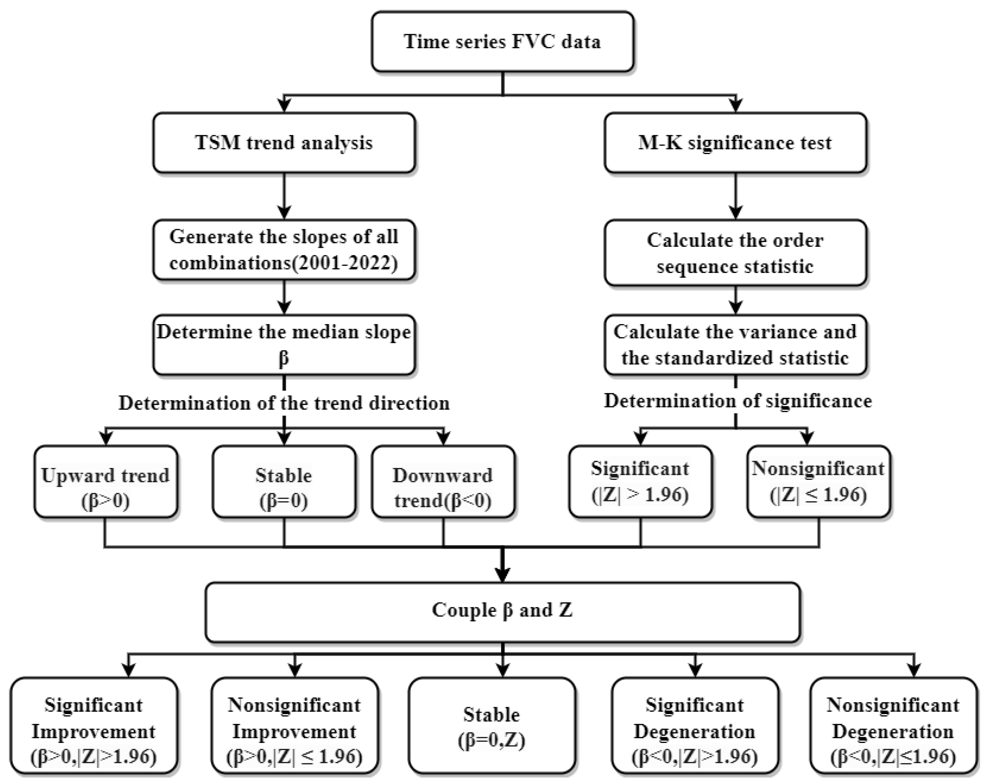
2.3.3. TSM and M-K Trend Analysis
2.3.4. Hurst Exponent
- (1)
- Create a pixel time series (Vt), where t ranging from 1 to n.
- (2)
- Mean value calculation:
- (3)
- Cumulative fluctuation series:
- (4)
- Range calculation:
- (5)
- Standard deviation calculation:
- (6)
- Hurst exponent calculation:
2.3.5. Geographical Detector
- (1)
- Factor Detection
- (2)
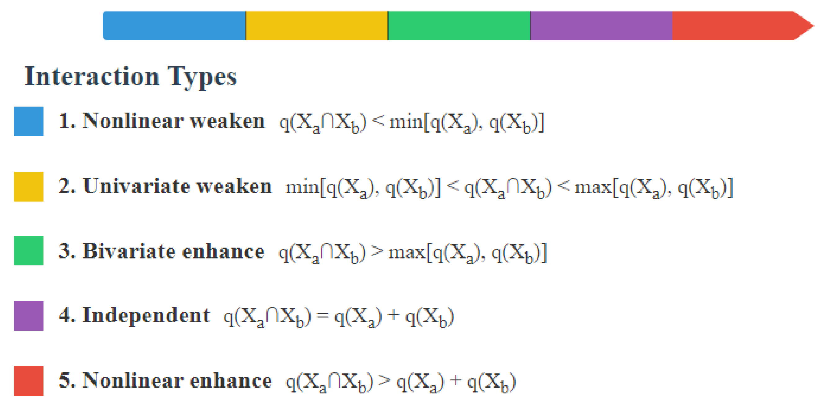
- Interaction Detection
- (3)
- Risk Detection
3. Results
3.1. Verification of FVC in the LRB
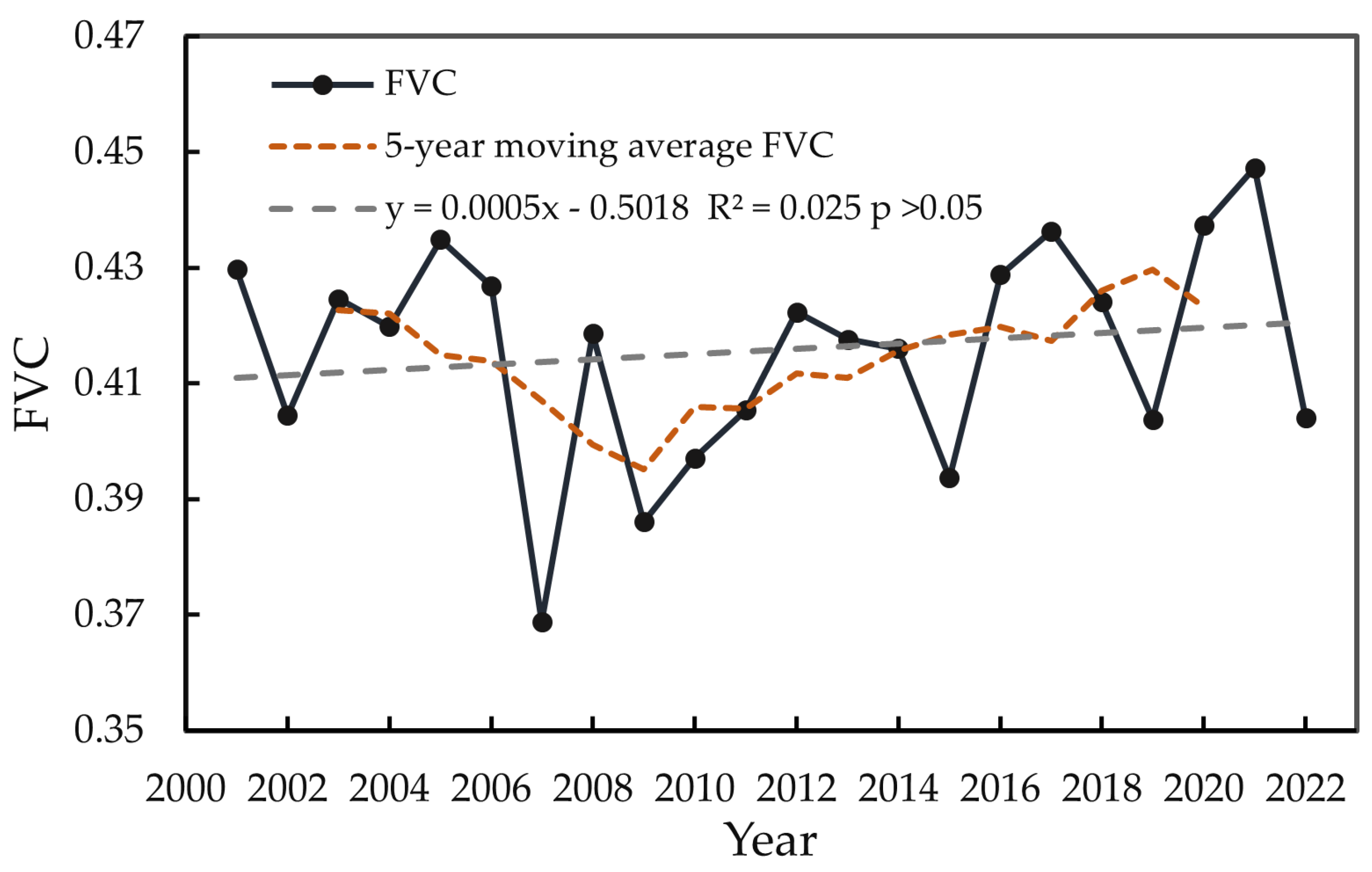
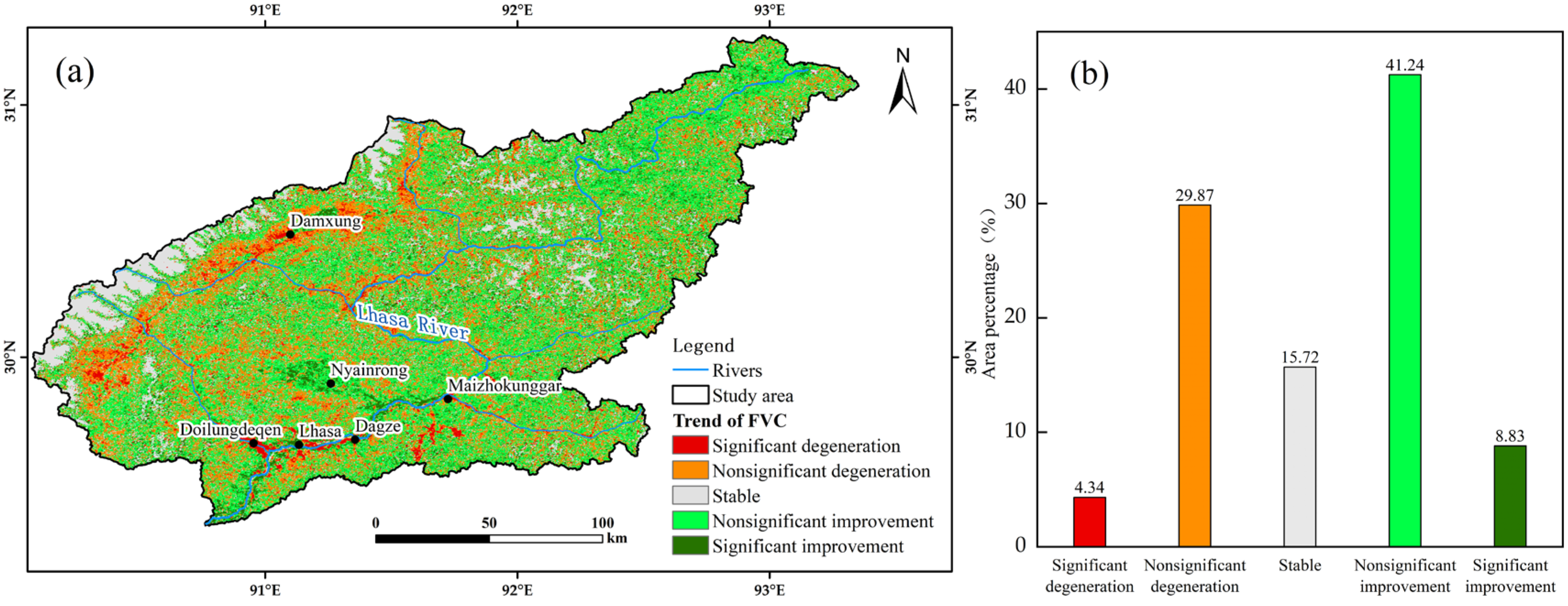
3.2. Spatiotemporal Variation of FVC in the LRB
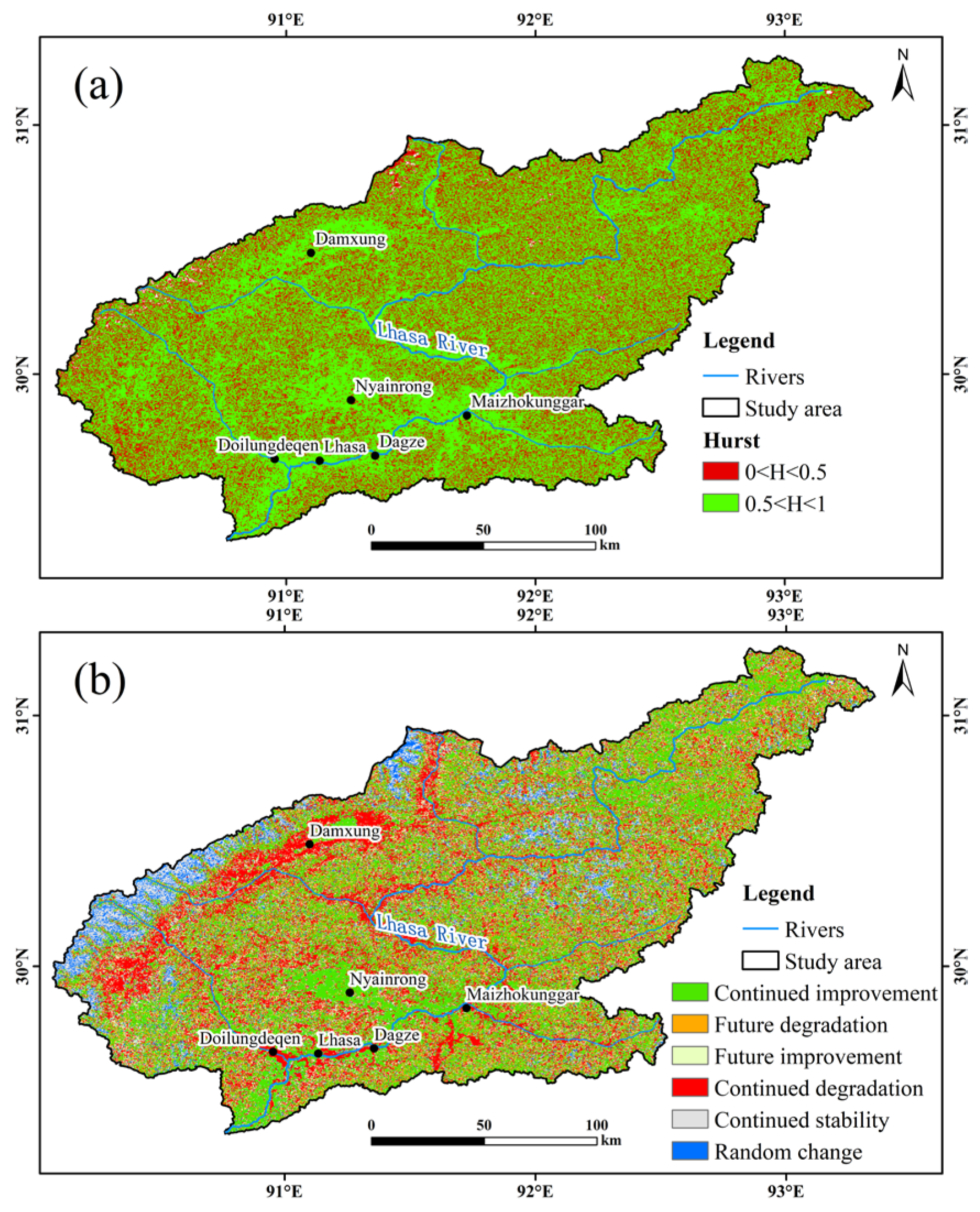
3.3. Sustainability of FVC in the LRB
3.4. Driving Factors of FVC in the LRB
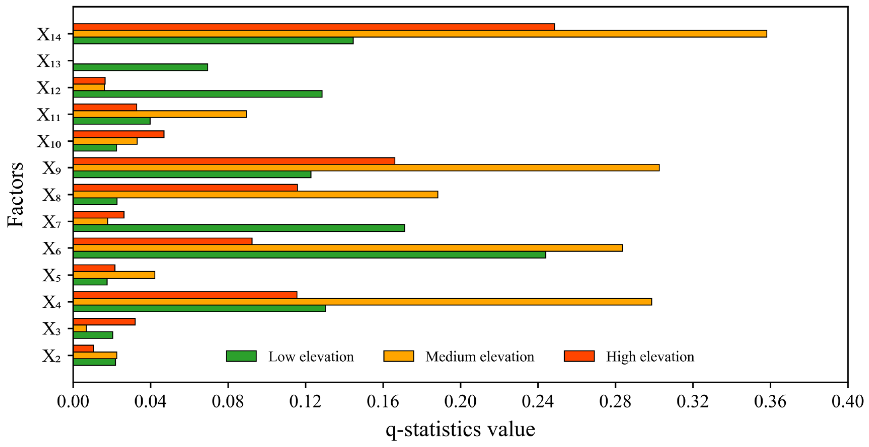
3.4.1. Factor Detection Analysis
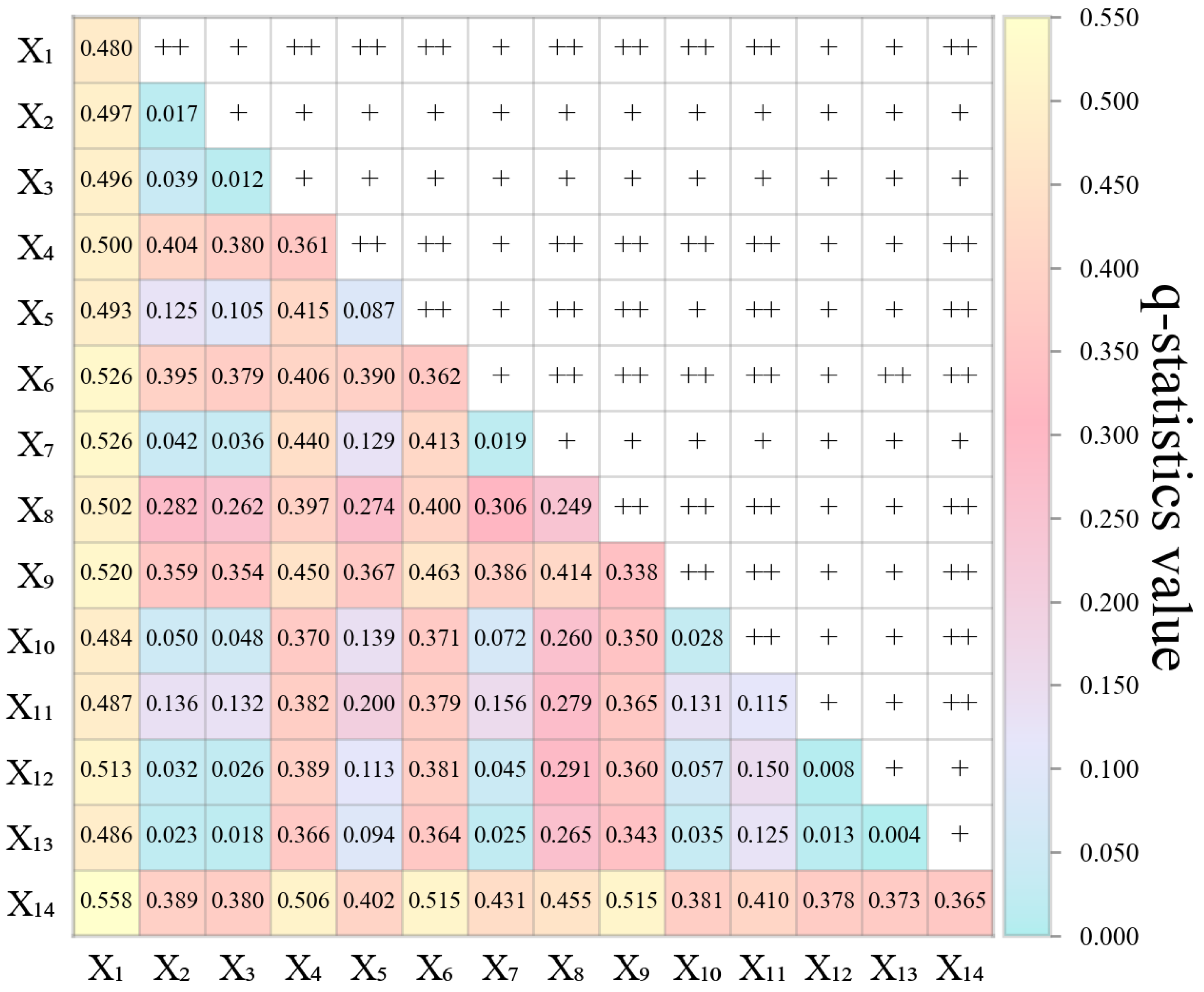
3.4.2. Interaction Detection Analysis
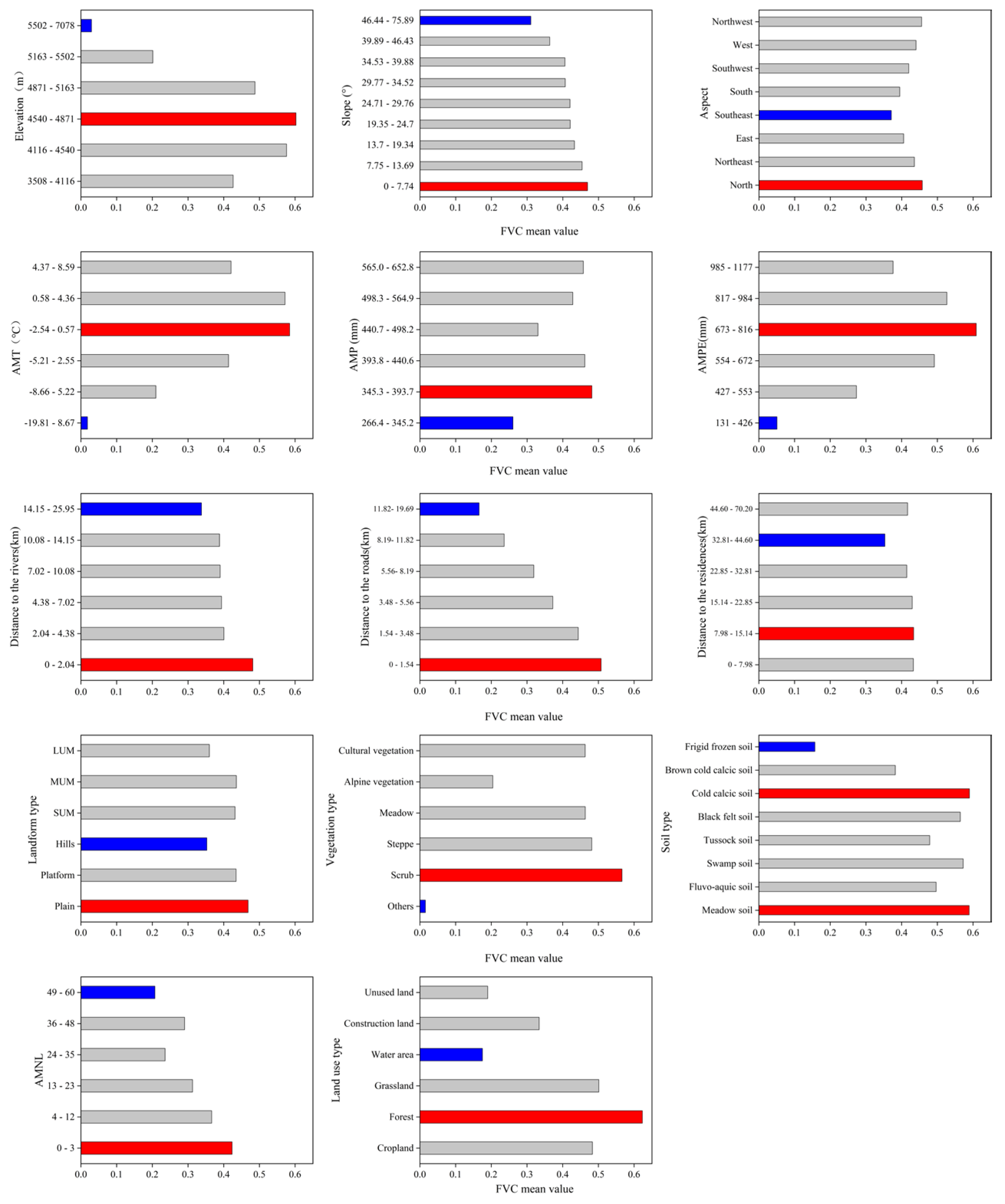
3.4.3. Risk Detection
4. Discussion
4.1. Spatiotemporal Variation of FVC
4.2. Driving Forces of Vegetation Change
4.2.1. Natural Factors
4.2.2. Human Factors
4.2.3. Impact of Factor Interactions on FVC
4.3. Limitations and Prospects
5. Conclusions
Author Contributions
Funding
Data Availability Statement
Conflicts of Interest
References
- Piao, S.; Wang, X.; Park, T. Characteristics, drivers and feedbacks of global greening. Nat. Rev. Earth Environ. 2020, 1, 14–27. [Google Scholar] [CrossRef]
- Deng, H.; Chen, Y.; Chen, X.; Li, Y.; Ren, Z.; Zhang, Z.; Zheng, Z.; Hong, S. The interactive feedback mechanisms between terrestrial water storage and vegetation in the Tibetan Plateau. Front. Earth Sci. 2022, 10, 1004846. [Google Scholar] [CrossRef]
- Liu, Y.; Xie, Y.; Guo, Z.; Xi, G. Effects of Climate Variability and Human Activities on Vegetation Dynamics across the Qinghai–Tibet Plateau from 1982 to 2020. Remote Sens. 2023, 15, 4988. [Google Scholar] [CrossRef]
- Chen, X.; Guan, T.; Zhang, J.; Liu, Y.; Jin, J.; Liu, C.; Wang, G.; Bao, Z. Identifying and Predicting the Responses of Multi-Altitude Vegetation to Climate Change in the Alpine Zone. Forests 2024, 15, 308. [Google Scholar] [CrossRef]
- Zhao, D.; Wang, Z.; Wu, X.; Qiu, T. Response of vegetation dynamics in environmentally sensitive and fragile areas to natural and anthropogenic factors: A case study in Inner Mongolia Autonomous Region, China. Anthropocene 2023, 44, 100414. [Google Scholar] [CrossRef]
- Zhang, S.; Zhou, Y.; Yu, Y.; Li, F.; Zhang, R.; Li, W. Using the Geodetector Method to Characterize the Spatiotemporal Dynamics of Vegetation and Its Interaction with Environmental Factors in the Qinba Mountains, China. Remote Sens. 2022, 14, 5794. [Google Scholar] [CrossRef]
- Pei, J.; Wang, L.; Huang, H.; Wang, L.; Li, W.; Wang, X.; Yang, H.; Cao, J.; Fang, H.; Niu, Z. Characterization and attribution of vegetation dynamics in the ecologically fragile South China Karst: Evidence from three decadal Landsat observations. Front. Plant Sci. 2022, 13, 1043389. [Google Scholar] [CrossRef]
- Zhang, S.; Ye, L.; Huang, C.; Wang, M.; Yang, Y.; Wang, T.; Tan, W. Evolution of vegetation dynamics and its response to climate in ecologically fragile regions from 1982 to 2020: A case study of the Three Gorges Reservoir area. Catena 2022, 219, 106601. [Google Scholar] [CrossRef]
- Li, W.; Yan, D.; Weng, B.; Lai, Y.; Zhu, L.; Qin, T.; Dong, Z.; Bi, W. Nonlinear effects of surface soil moisture changes on vegetation greenness over the Tibetan plateau. Remote Sens. Environ. 2024, 302, 113971. [Google Scholar] [CrossRef]
- Feng, Z.; Chen, J.; Huang, R.; Yang, Y.; You, H.; Han, X. Spatial and Temporal Variation in Alpine Vegetation Phenology and Its Response to Climatic and Topographic Factors on the Qinghai–Tibet Plateau. Sustainability 2022, 14, 12802. [Google Scholar] [CrossRef]
- Xu, B.; Li, J.; Pei, X.; Bian, L.; Zhang, T.; Yi, G.; Bie, X.; Peng, P. Dominance of Topography on Vegetation Dynamics in the Mt. Qomolangma National Nature Reserve: A UMAP and PLS-SEM Analysis. Forests 2023, 14, 1415. [Google Scholar] [CrossRef]
- Huang, R.; Chen, J.; Feng, Z.; Yang, Y.; You, H.; Han, X. Fitness for Purpose of Several Fractional Vegetation Cover Products on Monitoring Vegetation Cover Dynamic Change—A Case Study of an Alpine Grassland Ecosystem. Remote Sens. 2023, 15, 1312. [Google Scholar] [CrossRef]
- Liu, X.; Lu, H.; Yang, K.; Xu, Z.; Wang, J. Responses of runoff processes to vegetation dynamics during 1981–2010 in the Yarlung Zangbo River basin. J. Hydrol. Reg. Stud. 2023, 50, 101553. [Google Scholar] [CrossRef]
- Wu, K.; Hu, Z.; Wang, X.; Chen, J.; Yang, H.; Yuan, W. Widespread increase in sensitivity of vegetation growth to climate variability on the Tibetan Plateau. Agric. For. Meteorol. 2024, 358, 110260. [Google Scholar] [CrossRef]
- Liu, K.; Wang, X.; Wang, H. Quantifying the Contributions of Vegetation Dynamics and Climate Factors to the Enhancement of Vegetation Productivity in Northern China (2001–2020). Remote Sens. 2024, 16, 3813. [Google Scholar] [CrossRef]
- Carlson, T.N.; Ripley, D.A.J. On the relation between NDVI, fractional vegetation cover, and leaf area index. Remote Sens. Environ. 1997, 62, 241–252. [Google Scholar] [CrossRef]
- Xiao, J.; Moody, A. A comparison of methods for estimating fractional green vegetation cover within a desert-to-upland transition zone in central New Mexico, USA. Remote Sens. Environ. 2005, 98, 237–250. [Google Scholar] [CrossRef]
- Jia, K.; Liang, S.; Liu, S.; Li, Y.; Xiao, Z.; Yao, Y.; Jiang, B.; Zhao, X.; Wang, X.; Xu, S.; et al. Global Land Surface Fractional Vegetation Cover Estimation Using General Regression Neural Networks From MODIS Surface Reflectance. IEEE Trans. Geosci. Remote Sens. 2015, 53, 4787–4796. [Google Scholar] [CrossRef]
- Xiao, Z.; Liang, S.; Wang, J.; Chen, P.; Yin, X.; Zhang, L.; Song, J. Use of General Regression Neural Networks for Generating the GLASS Leaf Area Index Product From Time-Series MODIS Surface Reflectance. IEEE Trans. Geosci. Remote Sens. 2014, 52, 209–223. [Google Scholar] [CrossRef]
- Xiao, Z.; Wang, T.; Liang, S.; Sun, R. Estimating the Fractional Vegetation Cover from GLASS Leaf Area Index Product. Remote Sens. 2016, 8, 337. [Google Scholar] [CrossRef]
- Yang, L.; Jia, K.; Liang, S.; Liu, J.; Wang, X. Comparison of Four Machine Learning Methods for Generating the GLASS Fractional Vegetation Cover Product from MODIS Data. Remote Sens. 2016, 8, 682. [Google Scholar] [CrossRef]
- Xiao, Z.; Song, J.; Yang, H.; Sun, R.; Li, J. A 250 m resolution global leaf area index product derived from MODIS surface reflectance data. Int. J. Remote Sens. 2022, 43, 1409–1429. [Google Scholar] [CrossRef]
- Xiao, Z.; Liang, S.; Jiang, B. Evaluation of four long time-series global leaf area index products. Agric. For. Meteorol. 2017, 246, 218–230. [Google Scholar] [CrossRef]
- Zhang, Y.; Ye, A. Quantitatively distinguishing the impact of climate change and human activities on vegetation in mainland China with the improved residual method. GISci. Remote Sens. 2021, 58, 235–260. [Google Scholar] [CrossRef]
- Li, Y.; Song, Y.; Cao, X.; Huang, L.; Zhu, J. Temporal-Spatial Changes in Vegetation Coverage under Climate Change and Human Activities: A Case Study of Central Yunnan Urban Agglomeration, China. Sustainability 2024, 16, 661. [Google Scholar] [CrossRef]
- Guo, Y.; Cheng, L.; Ding, A.; Yuan, Y.; Li, Z.; Hou, Y.; Ren, L.; Zhang, S. Geodetector model-based quantitative analysis of vegetation change characteristics and driving forces: A case study in the Yongding River basin in China. Int. J. Appl. Earth Obs. Geoinf. 2024, 132, 104027. [Google Scholar] [CrossRef]
- Shi, S.; Wang, P.; Zhan, X.; Han, J.; Guo, M.; Wang, F. Warming and increasing precipitation induced greening on the northern Qinghai-Tibet Plateau. Catena 2023, 233, 107483. [Google Scholar] [CrossRef]
- Liu, W.; Mo, X.; Liu, S.; Lu, C. Impacts of climate change on grassland fractional vegetation cover variation on the Tibetan Plateau. Sci. Total Environ. 2024, 939, 173320. [Google Scholar] [CrossRef]
- Wei, Y.; Lu, H.; Wang, J.; Wang, X.; Sun, J. Dual Influence of Climate Change and Anthropogenic Activities on the Spatiotemporal Vegetation Dynamics Over the Qinghai-Tibetan Plateau From 1981 to 2015. Earth’s Future 2022, 10, e2021EF002566. [Google Scholar] [CrossRef]
- Zhang, Y.; Li, T.; Wang, B. Decadal Change of the Spring Snow Depth over the Tibetan Plateau: The Associated Circulation and Influence on the East Asian Summer Monsoon. J. Clim. 2004, 17, 2780–2793. [Google Scholar] [CrossRef]
- Duan, H.; Huang, B.; Liu, S.; Guo, J.; Zhang, J. Impact of Extreme Climate Indices on Vegetation Dynamics in the Qinghai–Tibet Plateau: A Comprehensive Analysis Utilizing Long-Term Dataset. ISPRS Int. J. Geo-Inf. 2024, 13, 457. [Google Scholar] [CrossRef]
- Shen, M.; Piao, S.; Jeong, S.J.; Zhou, L.; Zeng, Z.; Ciais, P.; Chen, D.; Huang, M.; Jin, C.S.; Li, L.Z.; et al. Evaporative cooling over the Tibetan Plateau induced by vegetation growth. Proc. Natl. Acad. Sci. USA 2015, 112, 9299–9304. [Google Scholar] [CrossRef]
- Bai, T.; Liu, J.; Liu, H.; Ni, F.; Han, X.; Qiao, X.; Sun, X. Elevation-dependent patterns of temporally asymmetrical vegetation response to climate in an alpine basin on the Qinghai-Tibet Plateau. Ecol. Indic. 2024, 159, 111736. [Google Scholar] [CrossRef]
- Mukhtar, H.; Yang, Y.; Xu, M.; Wu, J.; Abbas, S.; Wei, D.; Zhao, W. Elevation-Dependent Vegetation Greening and Its Responses to Climate Changes in the South Slope of the Himalayas. Geophys. Res. Lett. 2025, 52, e2024GL113276. [Google Scholar] [CrossRef]
- Wang, L.; Zhang, L.; Xiao, Y.; Kong, L.; Ouyang, Z. Identifying suitable areas for cropland and urban development in the Qinghai-Tibet Plateau. Land Use Policy 2025, 150, 107462. [Google Scholar] [CrossRef]
- Guo, L.; Li, Y.; Luo, Y.; Gao, J.; Zhang, H.; Zou, Y.; Wu, S. The Compound Effects of Highway Reconstruction and Climate Change on Vegetation Activity over the Qinghai Tibet Plateau: The G318 Highway as a Case Study. Remote Sens. 2023, 15, 5473. [Google Scholar] [CrossRef]
- Bao, W.; Zhang, W.; Dong, J.; Yang, X.; Xia, S.; Chen, H. Impact of road corridors on soil properties and plant communities in high-elevation fragile ecosystems. Eur. J. For. Res. 2024, 143, 1717–1730. [Google Scholar] [CrossRef]
- Diao, C.; Liu, Y.; Zhao, L.; Zhuo, G.; Zhang, Y. Regional-scale vegetation-climate interactions on the Qinghai-Tibet Plateau. Ecol. Inform. 2021, 65, 101413. [Google Scholar] [CrossRef]
- Zhan, Q.; Zhao, W.; Yang, M.; Xiong, D. A long-term record (1995–2019) of the dynamics of land desertification in the middle reaches of Yarlung Zangbo River basin derived from Landsat data. Geogr. Sustain. 2021, 2, 12–21. [Google Scholar] [CrossRef]
- Nie, Y.; Zhang, X.; Yang, Y.; Liu, Z.; He, C.; Chen, X.; Lu, T. Assessing the impacts of historical and future land-use/cover change on habitat quality in the urbanizing Lhasa River Basin on the Tibetan Plateau. Ecol. Indic. 2023, 148, 110147. [Google Scholar] [CrossRef]
- Abudureheman, W.; Yusufujiang, R.; Zhang, F.; Rukeya, S.; Zhang, X. Temporal and spatial characteristics of grassland degradation in Xinjiang Section of Tianshan Mountains based on remote sensing monitoring and its relationship with climate factors. Pratacultural Sci. 2023, 40, 1779–1792. (In Chinese) [Google Scholar]
- Peng, S.; Ding, Y.; Wen, Z.; Chen, Y.; Cao, Y.; Ren, J. Spatiotemporal change and trend analysis of potential evapotranspiration over the Loess Plateau of China during 2011–2100. Agric. For. Meteorol. 2017, 233, 183–194. [Google Scholar] [CrossRef]
- Peng, S.; Gang, C.; Cao, Y.; Chen, Y. Assessment of climate change trends over the Loess Plateau in China from 1901 to 2100. Int. J. Climatol. 2018, 38, 2250–2264. [Google Scholar] [CrossRef]
- Peng, S.; Ding, Y.; Liu, W.; Zhi, L.I. 1 km monthly temperature and precipitation dataset for China from 1901 to 2017. Earth Syst. Sci. Data 2019, 11, 1931–1946. [Google Scholar] [CrossRef]
- Ding, Y.; Peng, S. Spatiotemporal trends and attribution of drought across China from 1901–2100. Sustainability 2020, 12, 477. [Google Scholar] [CrossRef]
- Ding, Y.; Peng, S. Spatiotemporal change and attribution of potential evapotranspiration over China from 1901 to 2100. Theor. Appl. Climatol. 2021, 145, 79–94. [Google Scholar] [CrossRef]
- Wu, Y.; Shi, K.; Chen, Z.; Liu, S.; Chang, Z. Developing improved time-series DMSP-OLS-like data (1992–2019) in China by integrating DMSP-OLS and SNPP-VIIRS. IEEE Trans. Geosci. Remote Sens. 2021, 60, 4407714. [Google Scholar] [CrossRef]
- Faul, F.; Erdfelder, E.; Buchner, A.; Lang, A.-G. Statistical power analyses using G*Power 3.1: Tests for correlation and regression analyses. Behav. Res. Methods 2009, 41, 1149–1160. [Google Scholar] [CrossRef]
- Zhang, L.; Zhang, H.; Sun, X.; Luo, L. Combined Use of Multiple Cloud-Free Snow Cover Products in China and Its High-Mountain Region: Implications From Snow Cover Identification to Snow Phenology Detection. Water Resour. Res. 2024, 60, e2023WR036274. [Google Scholar] [CrossRef]
- Zhang, Z.; Chang, J.; Xu, C.-Y.; Zhou, Y.; Wu, Y.; Chen, X.; Jiang, S.; Duan, Z. The response of lake area and vegetation cover variations to climate change over the Qinghai-Tibetan Plateau during the past 30 years. Sci. Total Environ. 2018, 635, 443–451. [Google Scholar] [CrossRef]
- Mann, H.B. Non-parametric tests against trend. Econometrica 1945, 13, 245. [Google Scholar] [CrossRef]
- Hurst, H.E. Long-Term Storage Capacity of Reservoirs. Trans. Am. Soc. Civ. Eng. 1951, 116, 770–799. [Google Scholar] [CrossRef]
- Ndayisaba, F.; Guo, H.; Bao, A.; Guo, H.; Karamage, F.; Kayiranga, A. Understanding the Spatial Temporal Vegetation Dynamics in Rwanda. Remote Sens. 2016, 8, 129. [Google Scholar] [CrossRef]
- Zhu, L.; Meng, J.; Zhu, L. Applying Geodetector to disentangle the contributions of natural and anthropogenic factors to NDVI variations in the middle reaches of the Heihe River Basin. Ecol. Indic. 2020, 117, 106545. [Google Scholar] [CrossRef]
- Lv, Y.; Xiu, L.; Yao, X.; Yu, Z.; Huang, X. Spatiotemporal evolution and driving factors analysis of the eco-quality in the Lanxi urban agglomeration. Ecol. Indic. 2023, 156, 111114. [Google Scholar] [CrossRef]
- Kang, Y.; Wang, Z.; Xu, B.; Shen, W.; Chen, Y.; Zhou, X.; Liu, Y.; Zhang, T.; Wang, G.; Jia, Y.; et al. Disentangling the Response of Vegetation Dynamics to Natural and Anthropogenic Drivers over the Minjiang River Basin Using Dimensionality Reduction and a Structural Equation Model. Forests 2024, 15, 1438. [Google Scholar] [CrossRef]
- Chang, Y.; Yang, C.; Xu, L.; Li, D.; Shang, H.; Gao, F. Analysis of Vegetation Dynamics and Driving Mechanisms on the Qinghai-Tibet Plateau in the Context of Climate Change. Water 2023, 15, 3305. [Google Scholar] [CrossRef]
- Li, J.; Wu, C.; Zhang, Y.; Penuelas, J.; Liu, L.; Ge, Q. Weakening warming on spring freeze-thaw cycle caused greening Earth’s third pole. Proc. Natl. Acad. Sci. USA 2024, 121, e2319581121. [Google Scholar] [CrossRef]
- Cheng, Y.; Yuan, Z.; Li, Y.; Fan, J.; Suo, M.; Wang, Y. The Influence of Different Climate and Terrain Factors on Vegetation Dynamics in the Lancang River Basin. Water 2022, 15, 19. [Google Scholar] [CrossRef]
- Liu, S.; Zhou, L.; Wang, H.; Lin, J.; Huang, Y.; Zhuo, P.; Ao, T. Development of Fractional Vegetation Cover Change and Driving Forces in the Min River Basin on the Eastern Margin of the Tibetan Plateau. Forests 2025, 16, 142. [Google Scholar] [CrossRef]
- Wang, X.; Cheng, G.; Zhao, T.; Zhang, X.; Zhu, L.; Huang, L. Assessment on protection and construction of ecological safety shelter for Tibet. Bull. Chin. Acad. Sci. (Chin. Version) 2017, 32, 29–34. [Google Scholar] [CrossRef]
- Wang, Q.; Ju, Q.; Wang, Y.; Fu, X.; Zhao, W.; Du, Y.; Jiang, P.; Hao, Z. Regional Patterns of Vegetation Dynamics and Their Sensitivity to Climate Variability in the Yangtze River Basin. Remote Sens. 2022, 14, 5623. [Google Scholar] [CrossRef]
- Zhang, X.; Jin, X. Vegetation dynamics and responses to climate change and anthropogenic activities in the Three-River Headwaters Region, China. Ecol. Indic. 2021, 131, 108223. [Google Scholar] [CrossRef]
- Zhao, Z.; Dai, E. Vegetation cover dynamics and its constraint effect on ecosystem services on the Qinghai-Tibet Plateau under ecological restoration projects. J. Environ. Manag. 2024, 356, 120535. [Google Scholar] [CrossRef]
- Zhang, L.; Yang, L.; Zohner, C.M.; Crowther, T.W.; Li, M.; Shen, F.; Guo, M.; Qin, J.; Yao, L.; Zhou, C. Direct and indirect impacts of urbanization on vegetation growth across the world’s cities. Sci. Adv. 2022, 8, eabo0095. [Google Scholar] [CrossRef]
- Peng, J.; Liu, Z.; Liu, Y.; Wu, J.; Han, Y. Trend analysis of vegetation dynamics in Qinghai–Tibet Plateau using Hurst Exponent. Ecol. Indic. 2012, 14, 28–39. [Google Scholar] [CrossRef]
- Li, H.; Song, W. Spatiotemporal Distribution and Influencing Factors of Ecosystem Vulnerability on Qinghai-Tibet Plateau. Int. J. Env. Res Public Health 2021, 18, 6508. [Google Scholar] [CrossRef]
- Peng, W.; Kuang, T.; Tao, S. Quantifying influences of natural factors on vegetation NDVI changes based on geographical detector in Sichuan, western China. J. Clean. Prod. 2019, 233, 353–367. [Google Scholar] [CrossRef]
- Xu, T.; Wu, H. Spatiotemporal Analysis of Vegetation Cover in Relation to Its Driving Forces in Qinghai-Tibet Plateau. Forests 2023, 14, 1835. [Google Scholar] [CrossRef]
- Maxwell, S.K.; Sylvester, K.M. Identification of “ever-cropped” land (1984–2010) using Landsat annual maximum NDVI image composites: Southwestern Kansas case study. Remote Sens Env. 2012, 121, 186–195. [Google Scholar] [CrossRef]
- Wang, Y.; Fu, B.; Liu, Y.; Li, Y.; Feng, X.; Wang, S. Response of vegetation to drought in the Tibetan Plateau: Elevation differentiation and the dominant factors. Agric. For. Meteorol. 2021, 306, 108468. [Google Scholar] [CrossRef]
- Li, M.; Wu, J.; Feng, Y.; Niu, B.; He, Y.; Zhang, X. Climate Variability Rather Than Livestock Grazing Dominates Changes in Alpine Grassland Productivity Across Tibet. Front. Ecol. Evol. 2021, 9, 631024. [Google Scholar] [CrossRef]
- Wang, Y.; Lv, W.; Xue, K.; Wang, S.; Zhang, L.; Hu, R.; Zeng, H.; Xu, X.; Li, Y.; Jiang, L.; et al. Grassland changes and adaptive management on the Qinghai–Tibetan Plateau. Nat. Rev. Earth Environ. 2022, 3, 668–683. [Google Scholar] [CrossRef]
- Li, X.; Liang, E.; Camarero, J.J.; Rossi, S.; Zhang, J.; Zhu, H.; Fu, Y.H.; Sun, J.; Wang, T.; Piao, S. Warming-induced phenological mismatch between trees and shrubs explains high-elevation forest expansion. Natl. Sci. Rev. 2023, 10, nwad182. [Google Scholar] [CrossRef]
- Huo, H.; Sun, C. Spatiotemporal variation and influencing factors of vegetation dynamics based on Geodetector: A case study of the northwestern Yunnan Plateau, China. Ecol. Indic. 2021, 130, 108005. [Google Scholar] [CrossRef]
- Zuo, D.; Han, Y.; Xu, Z.; Li, P.; Ban, C.; Sun, W.; Pang, B.; Peng, D.; Kan, G.; Zhang, R.; et al. Time-lag effects of climatic change and drought on vegetation dynamics in an alpine river basin of the Tibet Plateau, China. J. Hydrol. 2021, 600, 126532. [Google Scholar] [CrossRef]
- Chen, J.; Kuang, X.; Lancia, M.; Yao, Y.; Zheng, C. Analysis of the groundwater flow system in a high-altitude headwater region under rapid climate warming: Lhasa River Basin, Tibetan Plateau. J. Hydrol. Reg. Stud. 2021, 36, 100871. [Google Scholar] [CrossRef]
- Glanville, K.; Sheldon, F.; Butler, D.; Capon, S. Effects and significance of groundwater for vegetation: A systematic review. Sci. Total Environ. 2023, 875, 162577. [Google Scholar] [CrossRef]
- Kim, J.H.; Jackson, R.B. A Global Analysis of Groundwater Recharge for Vegetation, Climate, and Soils. Vadose Zone J. 2012, 11, vzj2011.0021RA. [Google Scholar] [CrossRef]
- Sherwood Lollar, B.; Warr, O.; Higgins, P.M. The Hidden Hydrogeosphere: The Contribution of Deep Groundwater to the Planetary Water Cycle. Annu. Rev. Earth Planet. Sci. 2024, 52, 443–466. [Google Scholar] [CrossRef]
- Fan, Y.; Miguez-Macho, G.; Jobbágy, E.G.; Jackson, R.B.; Otero-Casal, C. Hydrologic regulation of plant rooting depth. Proc. Natl. Acad. Sci. USA 2017, 114, 10572–10577. [Google Scholar] [CrossRef] [PubMed]
- Liang, Y.; Song, W. Ecological and Environmental Effects of Land Use and Cover Changes on the Qinghai-Tibetan Plateau: A Bibliometric Review. Land 2022, 11, 2163. [Google Scholar] [CrossRef]
- Zhu, Q.; Chen, H.; Peng, C.; Liu, J.; Piao, S.; He, J.-S.; Wang, S.; Zhao, X.; Zhang, J.; Fang, X.; et al. An early warning signal for grassland degradation on the Qinghai-Tibetan Plateau. Nat. Commun. 2023, 14, 6406. [Google Scholar] [CrossRef] [PubMed]
- Dai, E.; Zhao, Z.; Jia, L.; Jiang, X. Contribution of ecosystem services improvement on achieving Sustainable development Goals under ecological engineering projects on the Qinghai-Tibet Plateau. Ecol. Eng. 2024, 199, 107146. [Google Scholar] [CrossRef]
- Li, D.; Tian, P.; Luo, H.; Hu, T.; Dong, B.; Cui, Y.; Khan, S.; Luo, Y. Impacts of land use and land cover changes on regional climate in the Lhasa River basin, Tibetan Plateau. Sci. Total Environ. 2020, 742, 140570. [Google Scholar] [CrossRef]
- Monasterolo, M.; Poggio, S.L.; Medan, D.; Devoto, M. Wider road verges sustain higher plant species richness and pollinator abundance in intensively managed agroecosystems. Agric. Ecosyst. Environ. 2020, 302, 107084. [Google Scholar] [CrossRef]
- Chen, A.; Xu, C.; Zhang, M.; Guo, J.; Xing, X.; Yang, D.; Xu, B.; Yang, X. Cross-scale mapping of above-ground biomass and shrub dominance by integrating UAV and satellite data in temperate grassland. Remote Sens. Environ. 2024, 304, 114024. [Google Scholar] [CrossRef]
- Zhou, Y.; Li, X.; Liu, Y. Land use change and driving factors in rural China during the period 1995–2015. Land Use Policy 2020, 99, 105048. [Google Scholar] [CrossRef]
- Nie, T.; Dong, G.; Jiang, X.; Lei, Y. Spatio-Temporal Changes and Driving Forces of Vegetation Coverage on the Loess Plateau of Northern Shaanxi. Remote Sens. 2021, 13, 613. [Google Scholar] [CrossRef]
- Cao, F.; Ge, Y.; Wang, J.-F. Optimal discretization for geographical detectors-based risk assessment. GISci. Remote Sens. 2013, 50, 78–92. [Google Scholar] [CrossRef]
- Van Deventer, H.; Linström, A.; Naidoo, L.; Job, N.; Sieben, E.J.J.; Cho, M.A. Comparison between Sentinel-2 and WorldView-3 sensors in mapping wetland vegetation communities of the Grassland Biome of South Africa, for monitoring under climate change. Remote Sens. Appl. Soc. Environ. 2022, 28, 100875. [Google Scholar] [CrossRef]
- Ganem, K.A.; Xue, Y.; Rodrigues, A.D.A.; Franca-Rocha, W.; Oliveira, M.T.D.; Carvalho, N.S.D.; Cayo, E.Y.T.; Rosa, M.R.; Dutra, A.C.; Shimabukuro, Y.E. Mapping South America’s Drylands through Remote Sensing—A Review of the Methodological Trends and Current Challenges. Remote Sens. 2022, 14, 736. [Google Scholar] [CrossRef]
- Hao, J.; Xu, G.; Luo, L.; Zhang, Z.; Li, H. Quantifying the relative contribution of natural and human factors to vegetation coverage variation in coastal wetlands in China. Catena 2020, 188, 104429. [Google Scholar] [CrossRef]
- Ren, D.; Cao, A. Analysis of the heterogeneity of landscape risk evolution and driving factors based on a combined GeoDa and Geodetector model. Ecol. Indic. 2022, 144, 108832. [Google Scholar] [CrossRef]


| Factor Type | Code | Factors | Unit | Original Resolution |
|---|---|---|---|---|
| Natural factors | X1 | Elevation | m | 30 m |
| X2 | Slope | ° | 30 m | |
| X3 | Aspect | ° | 30 m | |
| X4 | AMT | °C | 1 km | |
| X₅ | AMP | mm | 1 km | |
| X₆ | AMPE | mm | 1 km | |
| X₇ | Landform type | / | 1 km | |
| X8 | Vegetation type | / | 1 km | |
| X9 | Soil type | / | 1 km | |
| X10 | Distance to the rivers | km | 250 m | |
| Human factors | X11 | Distance to the roads | km | 250 m |
| X12 | Distance to the residences | km | 250 m | |
| X13 | AMNL | / | 1 km | |
| X14 | Land use type | / | 30 m |
| Remote Sensing | |||
|---|---|---|---|
| FVC ≤ 0.5 | FVC > 0.5 | ||
| Observation | FVC ≤ 0.5 | a | b |
| FVC > 0.5 | c | d | |
| Hurst | β | Future Change | Percentage |
|---|---|---|---|
| >0.5 | ≥0.0005 | Continued improvement | 36.91% |
| <0.5 | ≥0.0005 | Future degradation | 13.26% |
| <0.5 | β ≤ −0.0005 | Future improvement | 9.80% |
| >0.5 | β ≤ −0.0005 | Continued degradation | 24.51% |
| >0.5 | −0.0005 < β < 0.0005 | Continued stability | 8.88% |
| <0.5 | −0.0005 < β < 0.0005 | Random change | 6.64% |
| Time Period | Data Length | Areas with Future Improvement Trend | Mean Hurst Exponent |
|---|---|---|---|
| 2001–2022 | 22 years | 46.71% | 0.54 |
| 2007–2022 | 16 years | 50.76% | 0.52 |
| 2013–2022 | 10 years | 47.49% | 0.49 |
| Factor Type | Factors | FVC Suitable Range or Types | FVC |
|---|---|---|---|
| Natural factors | Elevation | 4540–4871 m | 0.60 |
| Slope | 0–7.74° | 0.47 | |
| Aspect | North | 0.46 | |
| AMT | −2.54–0.57 °C | 0.58 | |
| AMP | 345.3–393.7 mm | 0.48 | |
| AMPE | 673–816 mm | 0.61 | |
| Landform type | Plain | 0.47 | |
| Vegetation type | Scrub | 0.57 | |
| Soil type | Meadow soil, cold calcic soil | 0.59 | |
| Distance to the rivers | 0–2.03 km | 0.48 | |
| Human factors | Distance to the roads | 0–1.54 km | 0.51 |
| Distance to the residences | 7.98–15.1 km | 0.43 | |
| AMNL | 0–3 | 0.42 | |
| Land use type | Forest | 0.62 |
Disclaimer/Publisher’s Note: The statements, opinions and data contained in all publications are solely those of the individual author(s) and contributor(s) and not of MDPI and/or the editor(s). MDPI and/or the editor(s) disclaim responsibility for any injury to people or property resulting from any ideas, methods, instructions or products referred to in the content. |
© 2025 by the authors. Licensee MDPI, Basel, Switzerland. This article is an open access article distributed under the terms and conditions of the Creative Commons Attribution (CC BY) license (https://creativecommons.org/licenses/by/4.0/).
Share and Cite
Duan, Y.; Zhang, X.; Zhang, H.; Yang, B.; Zhao, Y.; Pu, C.; Xiao, Z.; Yuan, X.; Pu, X.; Luo, L. Synergistic Drivers of Vegetation Dynamics in a Fragile High-Altitude Basin of the Tibetan Plateau Using General Regression Neural Network and Geographical Detector. Remote Sens. 2025, 17, 1829. https://doi.org/10.3390/rs17111829
Duan Y, Zhang X, Zhang H, Yang B, Zhao Y, Pu C, Xiao Z, Yuan X, Pu X, Luo L. Synergistic Drivers of Vegetation Dynamics in a Fragile High-Altitude Basin of the Tibetan Plateau Using General Regression Neural Network and Geographical Detector. Remote Sensing. 2025; 17(11):1829. https://doi.org/10.3390/rs17111829
Chicago/Turabian StyleDuan, Yanghai, Xunxun Zhang, Hongbo Zhang, Bin Yang, Yanggang Zhao, Chun Pu, Zhiqiang Xiao, Xin Yuan, Xinming Pu, and Lun Luo. 2025. "Synergistic Drivers of Vegetation Dynamics in a Fragile High-Altitude Basin of the Tibetan Plateau Using General Regression Neural Network and Geographical Detector" Remote Sensing 17, no. 11: 1829. https://doi.org/10.3390/rs17111829
APA StyleDuan, Y., Zhang, X., Zhang, H., Yang, B., Zhao, Y., Pu, C., Xiao, Z., Yuan, X., Pu, X., & Luo, L. (2025). Synergistic Drivers of Vegetation Dynamics in a Fragile High-Altitude Basin of the Tibetan Plateau Using General Regression Neural Network and Geographical Detector. Remote Sensing, 17(11), 1829. https://doi.org/10.3390/rs17111829