Estimation of Tree Canopy Closure Based on U-Net Image Segmentation and Machine Learning Algorithms

Abstract

Canopy closure is a critical indicator reflecting forest structure, biodiversity, and ecological balance. This study proposes an estimation method integrating U-Net segmentation with machine learning, significantly improving accuracy through multi-source remote sensing data and feature selection. Covering eight U.S. continental states, the study utilized 13,000 stratified samples equally split for model training and validation. Four states were used to train models based on XGBoost, random forest (RF), LightGBM, and support vector machine (SVM), while the remaining four states served for validation. The results indicate that (1) U-Net effectively extracted tree crowns from aerial imagery to construct the sample dataset; (2) among the tested algorithms, XGBoost achieved the highest accuracy of 0.88 when incorporating Sentinel-1, Sentinel-2, vegetation indices, and land cover features, outperforming models using only Sentinel-2 data by 25.7%; and (3) XGBoost-estimated tree canopy cover (Model TCC) showed finer spatial details than the National Land Cover Database Tree Canopy Cover (NLCD TCC), with R² against the true tree canopy closure from U-Net (True TCC) up to 49.1% higher. This approach offers a cost-effective solution for regional-scale canopy monitoring.

1. Introduction

In the context of escalating global climate change and increasingly prominent ecological issues, forests, as one of the Earth’s key ecosystems, play an irreplaceable role in mitigating climate warming through their carbon sequestration function [1,2,3,4,5]. Canopy closure, as a core indicator for assessing the degree of forest canopy coverage, not only plays a crucial role in forest carbon sequestration but also holds a significant position in ecological research [6,7,8,9,10,11,12,13,14,15]. In regions where canopy closure is low and the ecological environment is relatively fragile, afforestation can be considered to improve the ecological environment and enhance carbon sequestration capacity. Conversely, in areas with high canopy closure and relatively stable ecological conditions, appropriate silvicultural management and ecological restoration measures can be implemented to maintain and enhance forest ecological functions based on the specific situation [16,17,18]. Moreover, canopy closure is widely used for dynamic monitoring of tree growth [19,20]. By regularly measuring canopy closure, researchers and forest managers can directly track tree growth rates, health status, and the evolutionary trends of stand structure [21,22]. Changes in canopy closure can sensitively reflect the combined effects of ecological factors such as light, water, and soil nutrients on tree growth. This, in turn, provides guidance for implementing scientifically sound forest management measures, such as adjusting stand density and optimizing species composition, to promote healthy tree growth and enhance the stability and productivity of forest ecosystems [23,24,25].

At present, methods for measuring canopy closure mainly include ground-based measurements, aerial surveys, and satellite-based measurements. Ground-based techniques, such as GRS densitometers, visual estimation methods, and the use of narrow-angle hemispherical photography, spherical densitometers, and wide-angle hemispherical photography, can directly and comprehensively capture forest canopy information [26,27,28,29,30,31,32,33,34]. However, these methods are constrained by limited coverage, high labor costs, difficult terrain, and specific geographical and resource conditions, resulting in low monitoring efficiency and limited applicability. Compared to ground-based measurements, aerial survey techniques, including aerial photogrammetry, visual observation methods, and grid sampling, significantly improve measurement efficiency and spatial coverage [35,36,37,38,39,40,41]. Nonetheless, aerial surveys also face challenges such as high costs, the need for specialized equipment and technical support, as well as limitations imposed by weather conditions and difficulties in identifying complex terrain and vegetation types. In recent years, satellite-based measurement techniques, particularly LiDAR, have become a research focus due to their wide coverage, strong real-time monitoring capabilities, and high degree of automation [13,42,43,44]. However, satellite-based techniques also face numerous challenges, such as data accuracy being susceptible to atmospheric interference and surface reflectance, the high cost of LiDAR equipment, and limited penetration ability in complex forest environments.

Against this background, the launch of the Earth observation satellites Sentinel-1 and Sentinel-2 by the European Space Agency (ESA) has opened up new possibilities for canopy closure estimation. These two satellites provide radar and optical data, respectively, which, when combined with advanced algorithms and models, enable high-precision estimation of canopy closure [45,46,47]. In recent years, researchers have integrated radar data from Sentinel-1 with optical data from Sentinel-2, significantly improving the monitoring accuracy and spatial coverage of canopy closure. This integration not only overcomes the limitations of traditional measurement methods but also greatly enhances the efficiency of forest structural information acquisition [45,46,47]. Furthermore, Sentinel-1 and Sentinel-2 have demonstrated substantial potential in other forestry applications, such as forest canopy height estimation and forest classification [48,49,50,51], providing scientific support for large-scale, real-time monitoring of forest resources.

Although existing traditional ground-based measurement methods ensure high accuracy, they are time-consuming, labor-intensive, and limited in coverage. Similarly, conventional aerial survey techniques are constrained by the need for specialized equipment and high costs, making large-scale applications difficult. In contrast, U-Net-based image segmentation technology allows for the precise extraction of tree crown information from high-resolution aerial imagery. This technique enables the efficient acquisition of key parameters such as tree crown contours and area, which can then be used to estimate tree canopy closure [52,53]. By overcoming the spatial and temporal limitations of traditional measurement methods, this approach not only enhances measurement efficiency and accuracy but also provides a new and effective means for large-scale studies of tree canopy closure.

This study proposes a method to improve the accuracy of tree canopy closure monitoring, offering a more cost-effective alternative compared to traditional techniques. The method employs U-Net image segmentation to precisely extract canopy information from high-resolution aerial images, which is then used to derive canopy closure as ground-truth data. On this basis, this study integrates multi-source remote sensing data, including Sentinel-1 and Sentinel-2, and applies four commonly used machine learning algorithms—XGBoost, RF, LightGBM, and SVM—to estimate canopy closure. After performance validation of these algorithms, the optimal model was identified, and its estimation results were compared with NLCD TCC on spatiotemporal scales, achieving an effective estimation of tree canopy closure.

2. Study Area and Data

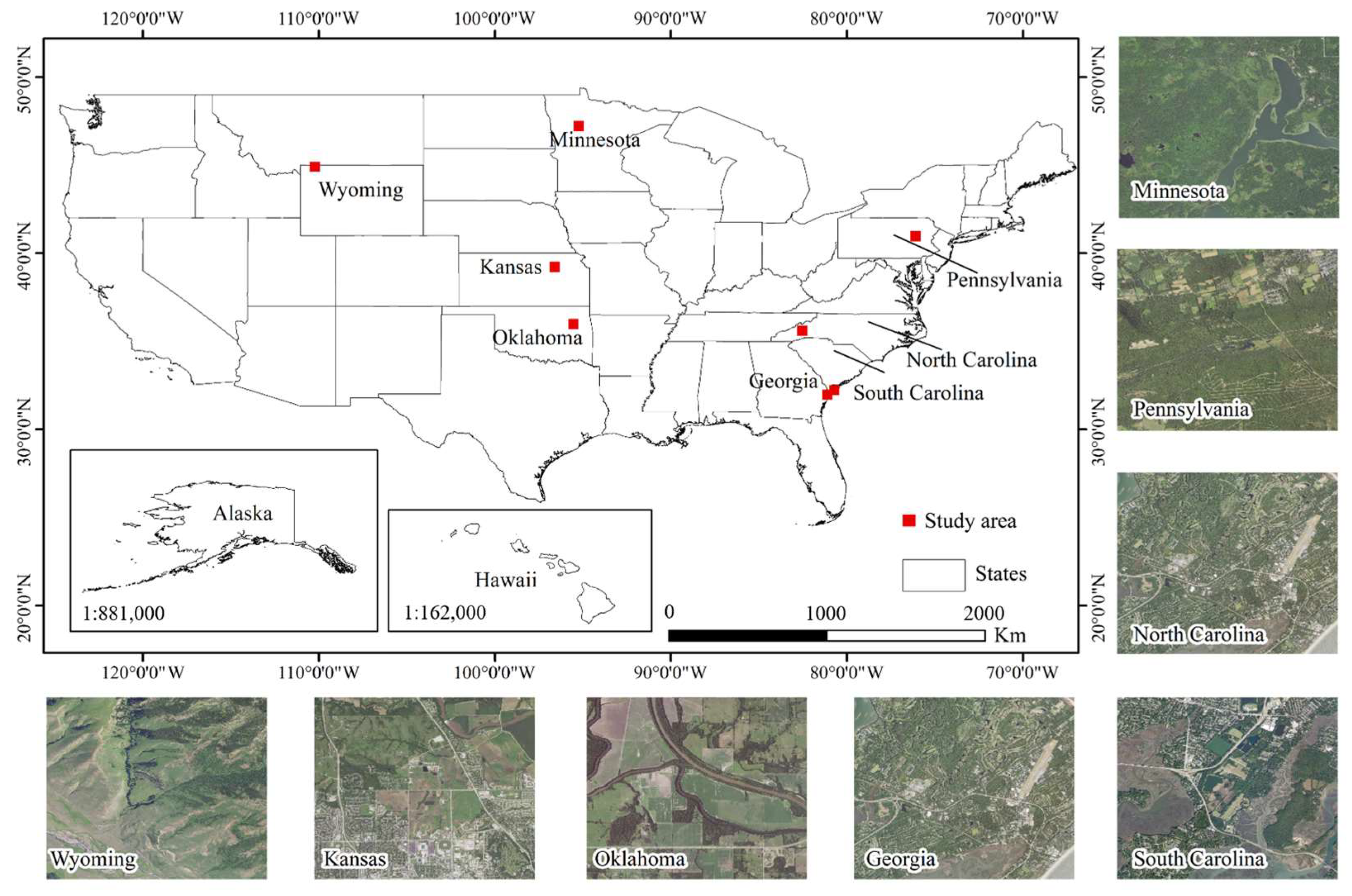
2.1. Study Area

The study areas in this research are distributed across eight states in the contiguous United States, specifically including Wyoming (WY) in the mountainous region; North Carolina (NC) and South Carolina (SC) along the southeastern Atlantic coast; Kansas (KS) and Oklahoma (OK) in the central Great Plains; Minnesota (MN) in the northwest-central region; Georgia (GA) in the South Atlantic region; and Pennsylvania (PA) in the Mid-Atlantic region. Each study area covers approximately 50 hectares, and the locations of the study areas are shown in Figure 1.

2.2. Acquisition and Preprocessing of Multi-Source Remote Sensing Data

2.2.1. Sentinel-1 Data

In this study, Sentinel-1 Ground Range Detected (GRD) data from Google Earth Engine (GEE) were preprocessed using the Sentinel-1 Toolbox. This process included key steps such as thermal noise removal, radiometric calibration, and terrain correction. In terms of data selection, only data from descending scenarios with vertical–vertical (VV) and vertical–horizontal (VH) polarization modes were utilized. To ensure the completeness and continuity of the time series, missing values in the Sentinel-1 data were filled using the average of the previous and subsequent years’ data for the same location.

2.2.2. Sentinel-2 Data

Since the Sentinel-2 Level-2A dataset only provided images of the study area for December 2018, to obtain a more comprehensive dataset, this study needed to expand the temporal scope. Therefore, all available Sentinel-2 MSI 1C level images from 2016 to 2021 were acquired. To ensure data quality and consistency while reducing data contamination due to cloud cover, images captured between 1 June and 31 August of each year with cloud cover below 10% were selected. Annual composite Sentinel-2 images were created by calculating the median of all eligible images during each year. Subsequently, the Sentinel-2 data underwent resampling, annual image compositing, and missing value imputation, following the same processing steps as the Sentinel-1 data.

2.2.3. National Agriculture Imagery Program (NAIP) Aerial Imagery

Using the code editor on GEE, a 0.6 m NAIP aerial imagery dataset from 2021 was selected for the specified study area to obtain high-resolution, broad coverage information for agricultural and natural areas, including the red, green, blue, and near-infrared (NIR) bands. Subsequently, the images were subjected to geometric correction, radiometric calibration, and atmospheric correction to ensure data quality and achieve precise extraction of the target image information.

2.2.4. NLCD TCC Product

The United States Forest Service (USFS) has developed two versions of tree canopy cover data to meet the needs of various user groups. These datasets cover the contiguous United States (CONUS), coastal Alaska, Hawaii, Puerto Rico, and the U.S. Virgin Islands (PRUSVI). The two versions of data in the v2021-4 TCC product suite include the initial model output, referred to as the scientific data, and a modified version constructed for the NLCD, known as the NLCD data. The NLCD product suite includes data for the years 2011, 2013, 2016, 2019, and 2021. Depending on the study area, the relevant NLCD TCC data can be downloaded from the USFS official website https://data.fs.usda.gov/geodata/rastergateway/treecanopycover (accessed on 5 August 2024).

2.2.5. Remote Sensing Vegetation Index

Vegetation indices enhance the spectral signal of vegetation, making tree canopies more prominent in imagery. The Normalized Difference Vegetation Index (NDVI) provides important information on forest ecosystems [54,55]. The Enhanced Vegetation Index (EVI) is widely used to assess forest cover changes, vegetation–temperature relationships, drought stress, and climate change impacts on forests [56,57,58]. The Normalized Difference Salinity Index (NDSI) helps monitor ion and water content in plant leaves, distinguishing healthy canopies from stressed ones [59]. The Normalized Difference Moisture Index (NDMI) estimates leaf biomass, water content, and cover density, aiding in canopy identification [60]. The Modified Soil Adjusted Vegetation Index (MSAVI) is effective for calculating canopy gap fraction, reflecting chlorophyll content under varying cover conditions with high resistance to soil and atmospheric interference [61,62]. The Green Red Vegetation Index (GRVI), similar to NDVI, uses the green channel to assess vegetation cover [63]. The vegetation indices used in the canopy closure estimation model in this paper are shown in

Table 1. Feature factors and descriptions of the canopy closure estimation model.

Feature	Descriptions	Feature	Descriptions
NDVI	${\displaystyle \frac{NIR-R}{NIR+R}}$	SAVI	$\left(1+L\right)\cdot {\displaystyle \frac{\mathit{NIR}-R}{\mathit{NIR}+R+L}}$
EVI	$\mathrm{G}\times {\displaystyle \frac{NIR-R}{NIR+C_1\times R-C_2\times B+L}}$	MSAVI	${\displaystyle \frac{2\cdot \left(NIR+1\right)-\sqrt{{\left(2\cdot NIR+1\right)}^2-8\cdot \left(NIR-R\right)}}{2}}$
NDFI	${\displaystyle \frac{\left(SWI{R}_1-R\right)-\left(SWI{R}_2-NIR\right)}{\left(SWI{R}_1-R\right)+\left(SWI{R}_2+NIR\right)}}$	ARVI	${\displaystyle \frac{\mathit{NIR}-\left(a\cdot R-b\cdot B\right)}{\mathit{NIR}+\left(a\cdot R-b\cdot B\right)}}$
GNDVI	${\displaystyle \frac{NIR-G}{NIR+G}}$	GRVI	${\displaystyle \frac{NIR-R}{NIR+R}}$
NDMI	${\displaystyle \frac{NIR-SWIR}{NIR+SWIR}}$	NBR	${\displaystyle \frac{NIR-SWIR}{NIR+SWIR}}$
NDSI	${\displaystyle \frac{G-SWIR}{G+SWIR}}$	DVI	$NIR-R$

, and these indices are part of the feature data used in the canopy closure estimation model discussed in this paper.

2.2.6. Auxiliary Data

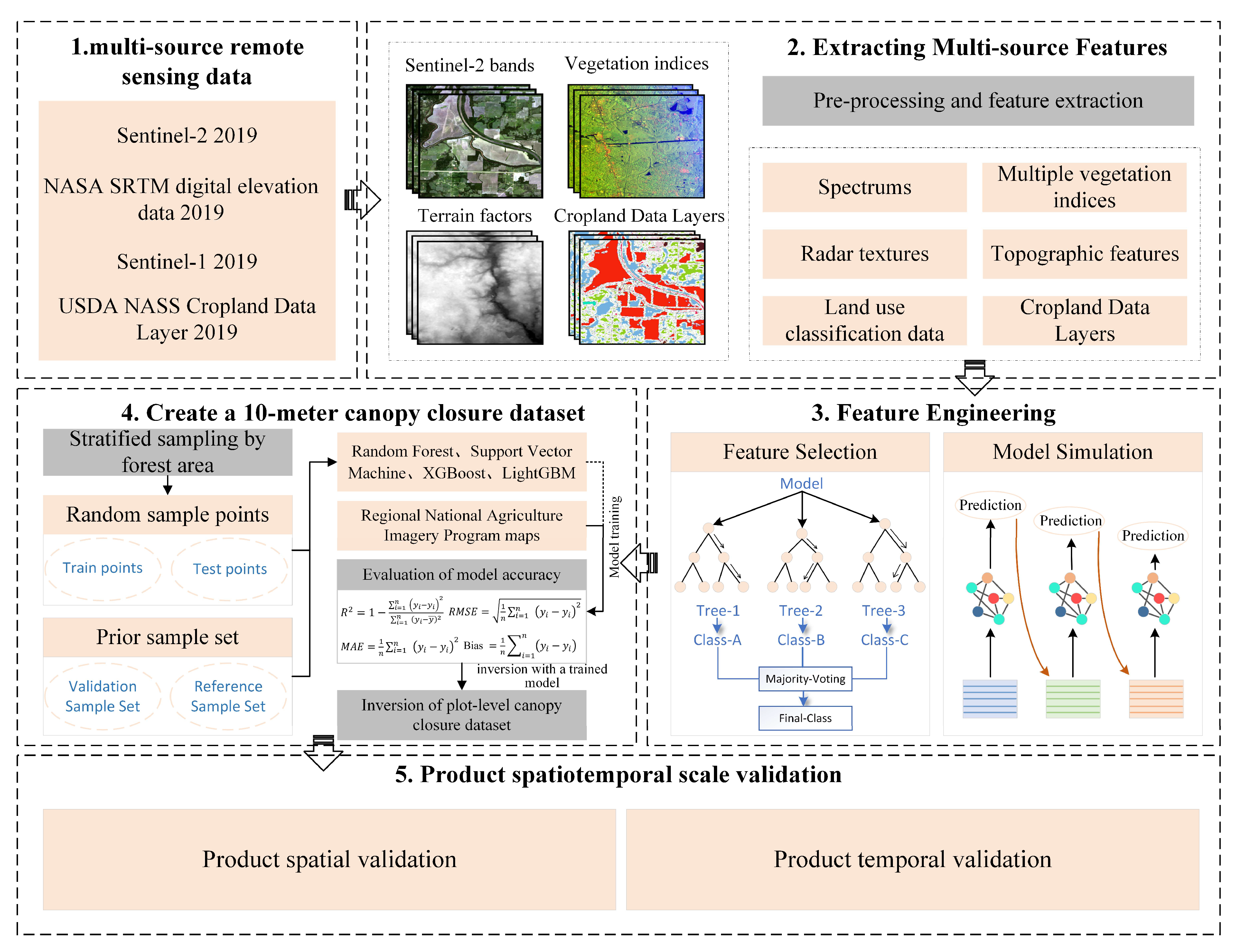
The auxiliary information used in this study includes a 30 m resolution Digital Elevation Model (DEM) product [64], a 30 m resolution Cropland Data Layer (CDL) [65], and a 10 m resolution ESA WorldCover land cover product [66]. All multi-source remote sensing data used for constructing the estimation model were acquired during the period from June to August 2021. This study specifically considers the potential impact of the cropland data layer on the identification of forest canopies in the study area. At the 30 m pixel level, surface crop type information is utilized to determine the canopy coverage and probability distribution of forests within the study area. The cropland data layer is generated by aggregating surface crop types into ten predefined land cover classes (i.e., cropland, grassland, forest, shrubland, wetland, water bodies, urban and built-up areas, bare areas, permanent snow and ice, and other agricultural land).

Additionally, the 10 m resolution ESA WorldCover land cover data for the study area was incorporated into the analysis. The ESA WorldCover product is a multi-year time series dataset that effectively supports studies on forest growth and change trends. This product has been processed with high accuracy, providing precise labels for various land cover types.

3. Methods

This study aims to develop an optimal forest canopy closure estimation model, with the methodological framework illustrated in Figure 2. First, canopy information is extracted from aerial imagery using U-Net image segmentation to obtain accurate canopy closure values. This is complemented by integrating multi-source remote sensing data, including Sentinel-2 and Sentinel-1, and applying correlation analysis and recursive feature elimination to optimize training features. Subsequently, four algorithms—XGBoost, RF, LightGBM, and SVM—are employed to construct the canopy closure estimation model. Finally, the estimation accuracy of the XGBoost model is evaluated through spatial and temporal analyses.

3.1. True Canopy Closure Modeling

This study employed the U-Net model for image segmentation based on the high-resolution characteristics of NAIP aerial imagery. During preprocessing, images were cropped into fixed 256 × 256 pixel windows and normalized for spectral consistency, enhancing model learning efficiency and stability. Data augmentation, including rotations, flips, and brightness/contrast adjustments, was applied to improve generalization. The U-Net model uses a classical encoder–decoder structure, with the encoder extracting spatial and semantic features and the decoder restoring resolution to generate segmentation masks. The loss function combines binary cross-entropy (BCE) and dice loss to address class imbalance. The model was trained with a learning rate of 1 × 10⁻⁴ using the Adam optimizer, completing training in 100 epochs with a batch size of 16. As shown in Figure 3, the U-Net model effectively captures edge details and regional connectivity, achieving an accuracy of 0.93, an mIoU of 0.89, and an F1 score of 0.83. The training and validation loss curves gradually converged without noticeable oscillation or overfitting, indicating good generalization performance. After obtaining the 0.6 m canopy mask results for the study area in 2021, spatial processing (including reclassification, block statistics, and resampling) is performed on this layer to generate 10 m resolution True TCC data. The entire process is illustrated in Figure 4.

To further improve the segmentation performance of the model in complex aerial imagery, this study adopted several strategies to address potential challenges. Firstly, to mitigate boundary blurring caused by overlapping tree crowns, edge enhancement techniques and multi-scale feature extraction were employed to capture spatial details. Additionally, the dice loss component in the hybrid loss function effectively focused on the segmentation of small regions and irregular tree crown boundaries. Secondly, considering the impact of varying illumination conditions on spectral information—particularly in regions with uneven lighting or pronounced shadows—adaptive normalization was introduced to dynamically adjust the spectral distribution. This was combined with brightness and contrast perturbations in data augmentation to simulate diverse environmental lighting conditions, thereby enhancing the model’s robustness. Finally, to alleviate recognition biases in high-spectral-complexity areas (e.g., mixed forests), resampling strategies and imbalanced data handling were integrated to ensure that the model sufficiently learned the characteristic distribution of different forest types during training. These improvements effectively enhanced the U-Net model’s generalization ability and spatial detail delineation in diverse environmental conditions, as validated in experimental evaluations.

3.2. Selection of Study Area Samples

To ensure that the sample points used to build and train the canopy cover model are both representative and reliable, this study employs a stratified sampling method [67]. A total of 13,000 sample points were selected across eight study areas for the training and validation datasets. Of these, 6686 sample points from the study areas of WY, KS, OK, and GA were used to train the model, while 6314 sample points from MN, PA, NC, and SC were used to validate the model. Subsequently, ESA WorldCover land use classification data were used to mask the tree TCC data and extract forested regions. Next, based on the natural breaks method and the national definition of forest canopy cover in China [68], the canopy cover values were categorized into three levels: 0.2–0.32, 0.32–0.76, and 0.76–1. Canopy closure values were categorized into three levels according to the natural breakpoint method and the definition of tree canopy closure in China, specifically 0.2–0.32, 0.32–0.76, and 0.76–1. Finally, to ensure the uniformity and objectivity of sample point selection, the number of sample points in each interval was set according to the proportion of the forest area in that interval relative to the total forest area of the study region, and sample points were randomly selected within each interval. This approach not only ensures an even distribution of sample points but also more accurately represents the forest distribution and canopy cover conditions in the study area. Details of the sample collection are shown in

Table 2. Statistical analysis of forest area and sample points by different levels of canopy closure in the study area.

	TCC	0.20–0.32	0.32–0.76	0.76–1.00
Study Area (km2)
WY		2.97/375 1	3.70/500	6.13/750
KS		4.43/432	3.46/329	7.75/864
OK		3.00/348	2.28/233	8.63/1044
GA		4.36/308	3.65/239	14.13/1078
MN		4.12/200	3.33/125	26.70/1300
PA		3.96/184	3.38/153	27.82/1288
NC		6.70/322	5.53/291	21.67/1012
SC		6.40/336	5.60/281	17.08/1008

¹ 2.97/750 represents the forest area (in km²)/number of forest sample points within the canopy cover interval of 0.2–0.32 in the WY study area.

. Furthermore, the spatial distribution of the specific sample points is illustrated in Figure 5.

3.3. Tree Canopy Closure Estimation Based on Machine Learning Models

3.3.1. Machine Learning Algorithms

In this study, four models were utilized: XGBoost, RF, LightGBM, and SVM. These models exhibit powerful capabilities in handling various data types, dealing with nonlinear relationships, and processing high-dimensional data. RF has strong resistance to overfitting and can successfully handle nonlinear relationships, but as the number of trees increases, the model can become more difficult to interpret. SVM has certain scalability issues and is highly sensitive to the choice of kernel functions. When selecting a machine learning model for a specific problem or dataset, these limitations need to be fully considered. XGBoost is efficient and scalable, playing a crucial role in preventing overfitting. LightGBM can reduce memory usage and accelerate training time. This study integrates these four models and compares their performance in estimating canopy cover to identify the model best suited for forest canopy cover estimation.

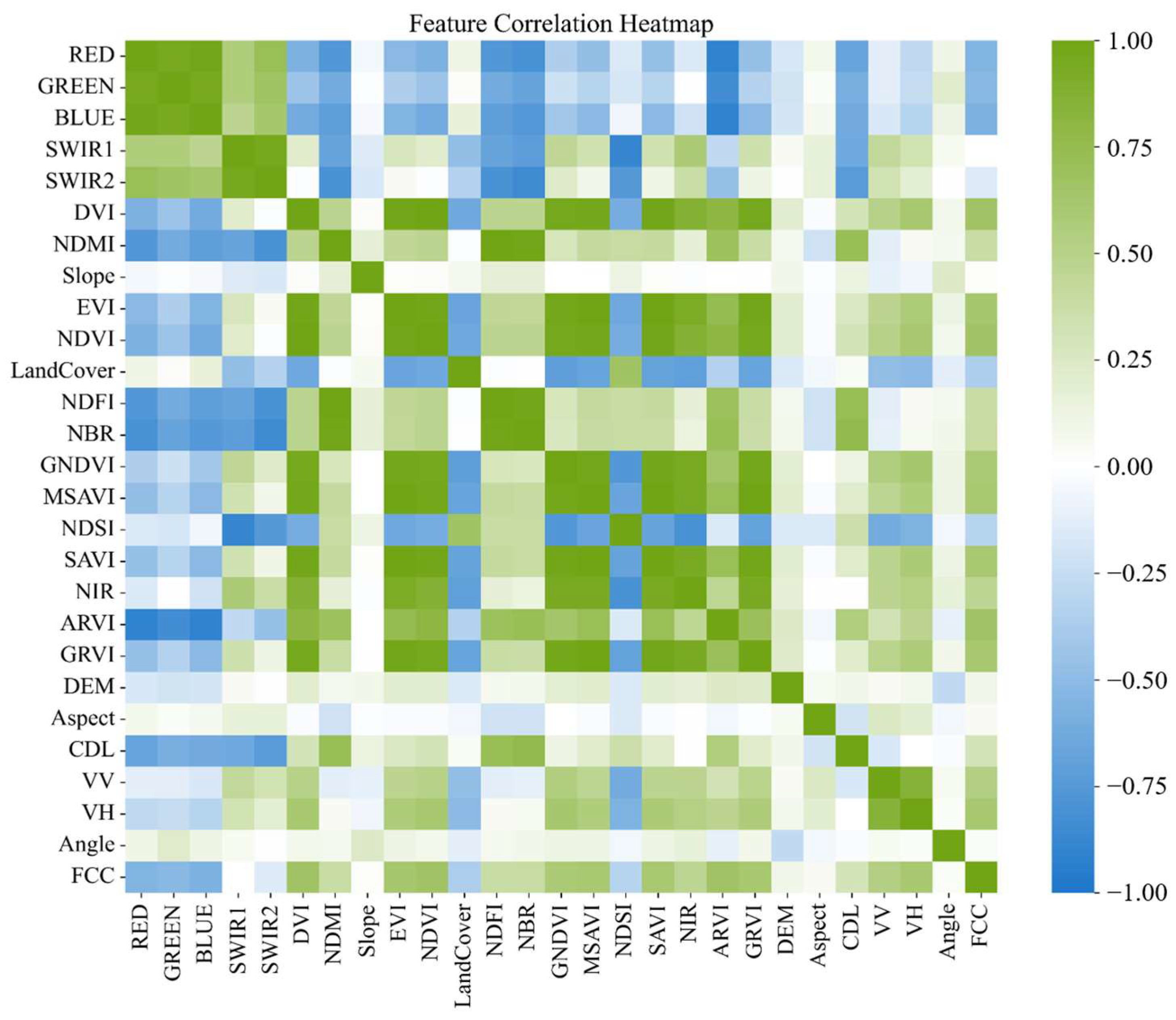
3.3.2. Feature Selection

In machine learning, the Pearson correlation coefficient (PCC) is a statistic used to measure the strength of the linear relationship between two continuous variables. It ranges from −1 to 1, where 1 indicates a perfect positive correlation: the variables show a perfect positive linear relationship; −1 indicates a perfect negative correlation: the variables show a perfect negative linear relationship; and 0 indicates no correlation: there is no linear relationship between the variables. The formula for the Pearson correlation coefficient is as follows:

$$\mathrm{r}={\displaystyle \frac{\sum _{\mathrm{i}=1}^{\mathrm{n}}\left({\mathrm{x}}_{\mathrm{i}}-\overline{\mathrm{x}}\right)\left({\mathrm{y}}_{\mathrm{i}}-\overline{\mathrm{y}}\right)}{\sqrt{\sum _{\mathrm{i}=1}^{\mathrm{n}}{\left({\mathrm{x}}_{\mathrm{i}}-\overline{\mathrm{x}}\right)}^2\sum _{\mathrm{i}=1}^{\mathrm{n}}{\left({\mathrm{y}}_{\mathrm{i}}-\overline{\mathrm{y}}\right)}^2}}}$$

(1)

where ${\mathrm{x}}_{\mathrm{i}}$ and ${\mathrm{y}}_{\mathrm{i}}$ are the values of two variables and $\overline{\mathrm{x}}$ and $\overline{\mathrm{y}}$ are the means of the two variables.

Feature selection is a crucial step in machine learning. By calculating the PCC between each feature and the target variable, we can identify and select features highly correlated with the target variable, thereby improving the predictive performance and generalization ability of the model. For example, if a feature has a correlation coefficient close to zero with the target variable, it may be considered for removal from the model as it contributes little to the prediction. Understanding the correlation between features is also important. Highly correlated features can lead to multicollinearity issues, affecting the stability and interpretability of the model. By computing the PCC between features, we can identify pairs of highly correlated features and mitigate multicollinearity effects through merging, transforming, or removing some features.

Feature importance analysis is a method used in machine learning to evaluate the extent to which each feature influences the model’s predictive results. Understanding feature importance aids in feature selection, model optimization, and interpretation, thereby improving model performance and interpretability. Random Forest trains and predicts by constructing multiple decision trees. Feature importance can be assessed by calculating the information gain brought by each feature in tree node splits, such as the Gini coefficient or reduction in entropy. For linear SVM, feature importance can be measured by weight coefficients (i.e., the coef_ attribute of the model). XGBoost, a gradient boosting tree model, provides various methods for assessing feature importance, such as weights, gains, and coverage. This paper employs recursive feature elimination (RFE) to compute feature importance, recursively training the model and eliminating features contributing least to the predictive target. Compared to simple filtering methods, RFE considers complex relationships between features, effectively reducing the feature space and enhancing the model’s generalization ability and interpretability.

3.3.3. Parameter Tuning

Grid search is a prevalent hyperparameter tuning technique applicable to a wide range of machine learning models, including XGBoost, RF, LightGBM, and SVM. Given that each model possesses specific parameters requiring adjustment, grid search systematically explores various parameter combinations to ascertain the optimal model performance. The process begins by defining the parameters that necessitate tuning and their respective value ranges. Subsequently, for each model, corresponding model instances and grid search with cross-validation (GridSearchCV) objects are created, with the parameter grid and the number of cross-validation folds (cv) being set. Following this, each model is fitted to search for the optimal parameter combination. The best parameters and corresponding scores for each model are then obtained, and the model performance is evaluated based on specific requirements.

3.3.4. Evaluation Metrics

This study selected four evaluation metrics to assess the training performance of regression models. These metrics include R squared (R²), root mean squared error (RMSE), mean absolute error (MAE), and bias. R² measures the goodness of fit of the model, ranging from 0 to 1, where values closer to 1 indicate better model fit. RMSE and MAE quantify the differences between simulated values and actual values, with smaller values indicating better model performance. Bias represents the average deviation between simulated and actual values and is an important indicator of model accuracy. These four evaluation metrics will be used comprehensively to assess the performance of the established regression models in predicting canopy closure. Through a comprehensive analysis of these metrics, a comprehensive understanding of the modeling capabilities, strengths, and weaknesses of the regression models in the study area can be obtained, providing a reliable basis and reference for the research.

$${\mathrm{R}}^2=1-{\displaystyle \frac{\sum _{\mathrm{i}=1}^{\mathrm{n}}{\left({\mathrm{y}}_{\mathrm{i}}-{\widehat{\mathrm{y}}}_{\mathrm{i}}\right)}^2}{\sum _{\mathrm{i}=1}^{\mathrm{n}}{\left({\mathrm{y}}_{\mathrm{i}}-\overline{\mathrm{y}}\right)}^2}}$$

(2)

$$\mathrm{R}\mathrm{M}\mathrm{S}\mathrm{E}=\sqrt{{\displaystyle \frac{1}{\mathrm{n}}}\sum _{\mathrm{i}=1}^{\mathrm{n}}{\left({\mathrm{y}}_{\mathrm{i}}-{\widehat{\mathrm{y}}}_{\mathrm{i}}\right)}^2}$$

(3)

$$\mathrm{M}\mathrm{A}\mathrm{E}={\displaystyle \frac{1}{\mathrm{n}}}\sum _{\mathrm{i}=1}^{\mathrm{n}}\left|{\mathrm{y}}_{\mathrm{i}}-{\widehat{\mathrm{y}}}_{\mathrm{i}}\right|$$

(4)

$$\mathrm{B}\mathrm{i}\mathrm{a}\mathrm{s}={\displaystyle \frac{1}{\mathrm{n}}}\sum _{\mathrm{i}=1}^{\mathrm{n}}\left({\widehat{\mathrm{y}}}_{\mathrm{i}}-{\mathrm{y}}_{\mathrm{i}}\right)$$

(5)

In the equations, ${\mathrm{y}}_{\mathrm{i}}$ represents the observed canopy closure value, ${\mathrm{y}}_{\mathrm{i}}$ represents the simulated canopy closure value, $\overline{\mathrm{y}}$ represents the average simulated value of the model, and n represents the total number of canopy closure samples.

3.4. Spatiotemporal Comparison of Canopy Closure Estimation Result

After training the XGBoost, RF, LightGBM, and SVM machine learning models, the XGBoost model with the best simulation performance was selected for a systematic spatiotemporal comparative analysis of estimated canopy closure results against NLCD TCC. At the spatial scale, visual comparisons were conducted between the 10 m resolution Model TCC and the True TCC, as well as between the 30 m resolution Model TCC, True TCC, and NLCD TCC, to reveal spatial distribution characteristics intuitively. Subsequently, Model TCC and NLCD TCC were, respectively, compared and validated against True TCC, with the coefficients of R², RMSE, MAE, and bias calculated to quantify estimation accuracy. At the temporal scale, canopy closure was estimated from 2016 to 2021, with comparative analyses conducted against NLCD TCC for corresponding years to examine temporal trends. These comparisons not only facilitate a comprehensive evaluation of the model’s accuracy and stability but also reveal the discrepancies between estimated and true values, thereby enabling an analysis of the potential factors influencing these differences.

4. Results and Analysis

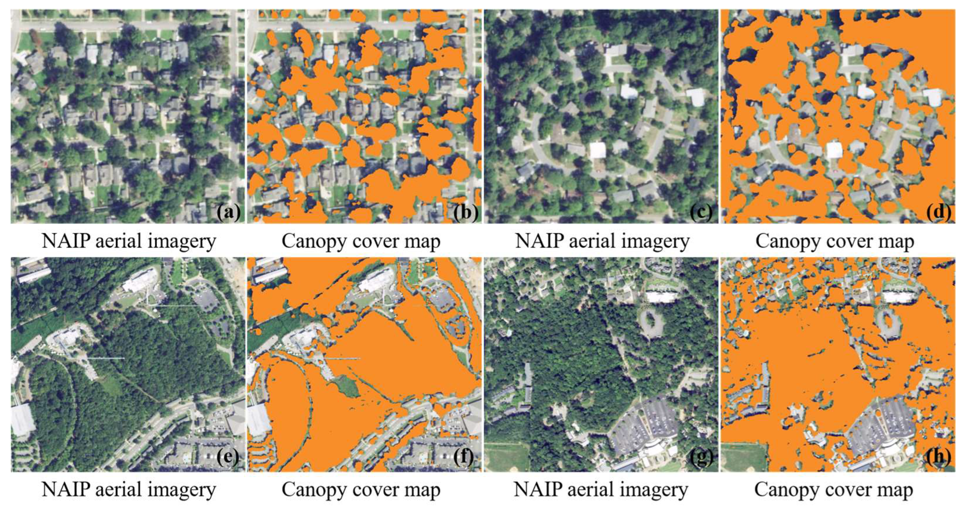
4.1. Crown Identification

This study utilized the 2021 NAIP aerial imagery to identify and extract canopy distribution maps and applied the Faster R-CNN object detection technique to recognize the canopies, successfully locating the positions and shapes of the canopies in the images. Subsequently, the U-Net image segmentation algorithm was employed to further refine the extraction and description of the boundaries and features of each canopy. Figure 6 presents four sets of images, with the left side showing the original NAIP aerial imagery and the right side displaying the corresponding canopy distribution maps. The extraction and analysis of these canopy data provide crucial real-world forest canopy closure information for the inversion of the canopy closure model.

4.2. Machine Learning-Based Estimation of Tree Canopy Closure

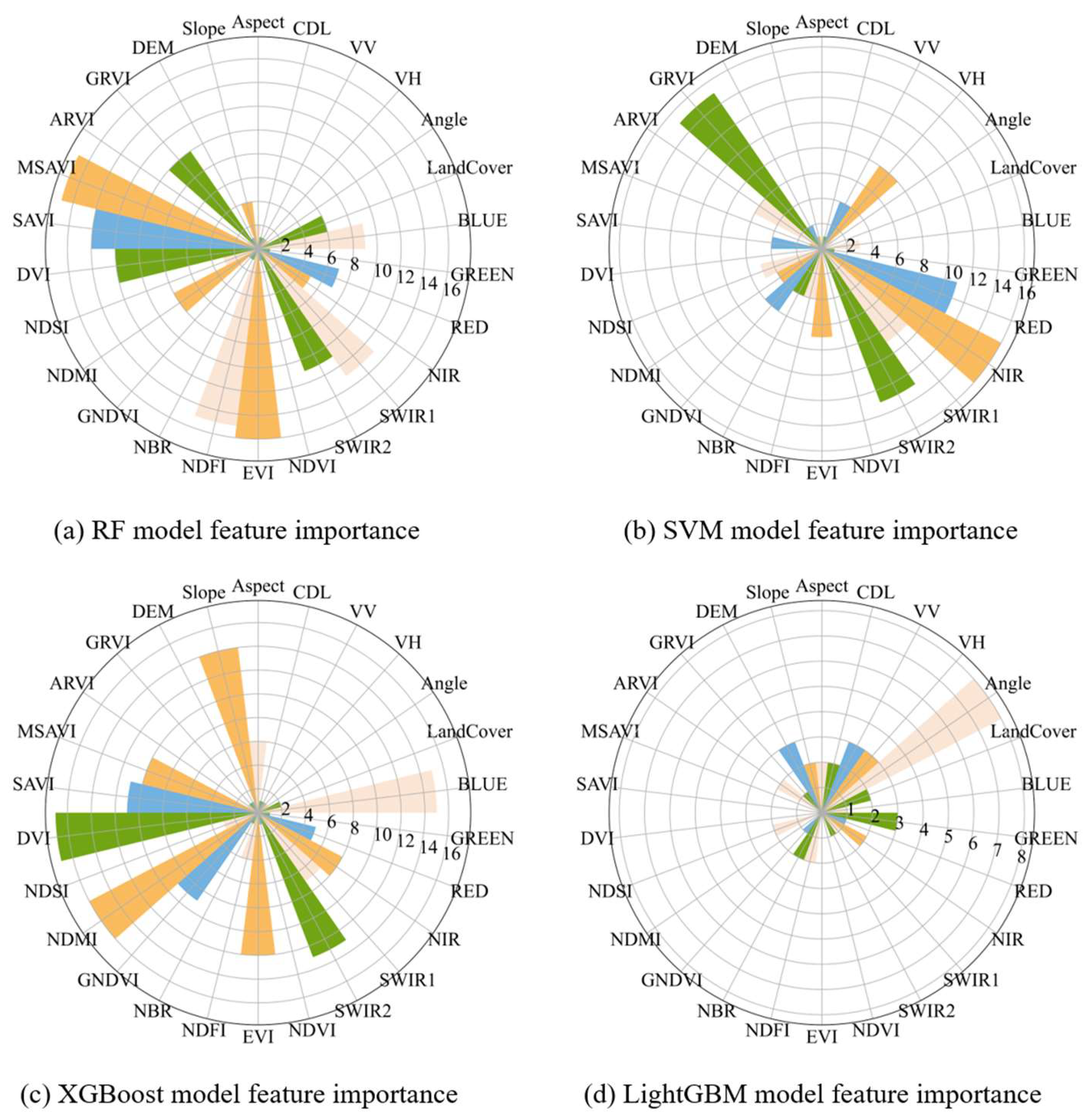
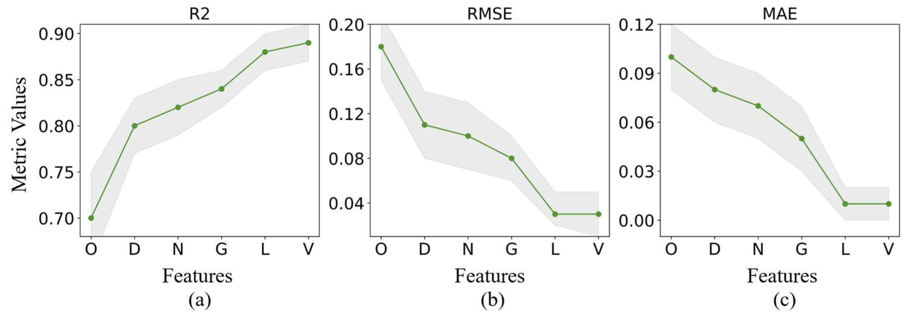
4.2.1. Feature Selection and Parameter Tuning

For the four machine learning models, this study first applied recursive feature elimination for feature selection to identify the ten most important features for each model. As shown in Figure 7, the key features for the RF model include MSAVI, SAVI, DVI, GRVI, NDFI, EVI, SWIR2, SWIR1, BLUE, and RED; for the SVM model, the key features are GRVI, SWIR2, SWIR1, NIR, RED, VH, EVI, GNDVI, ARVI, and NDSI; for the XGBoost ensemble model, the prominent features include DVI, NDMI, Slope, EVI, SWIR2, BLUE, Land-Cover, SAVI, MSAVI, and GNDVI; and for the LightGBM model, the key features are GNDVI, NDMI, GRVI, VV, BLUE, NIR, RED, NDVI, SWIR1, and EVI.

In the analysis of feature correlations, when the correlation coefficient between two features approaches 1 or −1, it indicates a strong linear relationship between them. To avoid multicollinearity issues, features with high correlation are typically removed during the feature selection process, retaining pairs of features with lower correlations to enhance the diversity and stability of the model. A high correlation (close to 1 or −1) with the target variable indicates a strong linear relationship between the feature and the target, reflecting the feature’s strong predictive ability for the target variable. Therefore, it is common practice to prioritize features with higher correlations with the target variable during feature selection.

To select the model with the best stability and predictive power, this study conducted a correlation analysis of the XGBoost model. As shown in Figure 8, the results reveal that DVI is strongly correlated with EVI, SAVI, and MSAVI. SAVI and MSAVI improve the accuracy of vegetation indices by incorporating soil adjustment factors to correct for the soil background’s impact, particularly in areas with exposed soil. EVI enhances the estimation of vegetation growth by introducing the reflectance of the red-edge band, making the index more sensitive and better able to differentiate between various types of vegetation. However, during feature selection, it was found that the correlations of EVI, SAVI, and MSAVI with FCC ground truth values were lower than that of DVI with FCC ground truth. Therefore, this study ultimately chose to retain the DVI feature to improve the model’s stability and predictive capacity.

Finally, the features used for training the RF model include MSAVI, Slope, LandCover, NDFI, VV, VH, BLUE, and RED; for the SVM model, the features are GRVI, RED, BLUE, NDSI, LandCover, NDMI, VV, and VH; for the XGBoost model, the features include DVI, NDMI, NDVI, SWIR2, BLUE, LandCover, GNDVI, and VH; and for the LightGBM model, the features include GNDVI, NDMI, VV, BLUE, RED, SWIR1, LandCover, and VH.

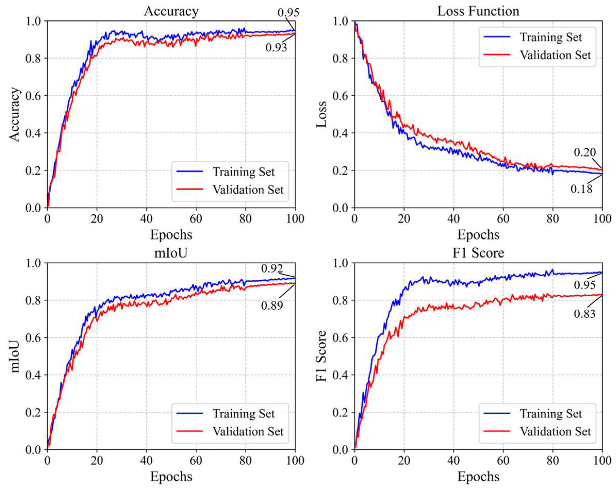
4.2.2. Model Estimation Accuracy

The simulation results of each model revealed certain differences in the performance metrics. Specifically, as shown in Figure 9, the R² values fluctuated between 0.62 and 0.89, the RMSE values ranged from 0.11 to 0.21, and the MAE values varied between 0.08 and 0.27. It is noteworthy that all models exhibited overestimation in the high-value range, with the regression line below the 1:1 line, and underestimation in the low-value range, with the regression line above the 1:1 line.

This study validated the XGBoost, RF, LightGBM, and SVM machine learning models using the true FCC values (Figure 9). Observation of the density heat map revealed that sample points with a canopy closure greater than 0.8 were concentrated in certain areas. This uneven distribution primarily resulted from the implementation of canopy closure stratified sampling during sample selection, leading to an imbalance in the area proportions of the strata. Specifically, sample points from areas with higher forest density were more frequent, while those from lower density areas were relatively scarce. Among these models, the SVM model exhibited significant bias. This could be attributed to the inability of the SVM model to adequately capture key information affecting canopy closure when using recursive feature elimination (RFE) for feature selection, leading to insufficient and unrepresentative input features. Furthermore, the number of samples across different strata varied considerably, resulting in an imbalanced data label distribution. As a result, the SVM model tended to favor the more numerous classes, exacerbating the model’s bias.

XGBoost demonstrates the highest estimation accuracy primarily due to its unique algorithmic design and optimization mechanisms. First, XGBoost is built upon the gradient boosting decision tree (GBDT) framework, where new trees are incrementally constructed to correct the residuals of the previous ones, thereby continuously improving the model’s fitting ability [69]. Compared to the parallel random sampling strategy of RF, XGBoost’s boosting mechanism focuses more on optimizing residuals, enabling it to capture nonlinear relationships and complex feature interactions more accurately [70]. Furthermore, XGBoost introduces regularization terms during model training, effectively preventing overfitting, which is particularly advantageous when handling high-dimensional and multi-feature remote sensing imagery, resulting in stronger generalization capabilities [71]. In addition, XGBoost supports custom loss functions and leverages a second-order Taylor expansion for accelerated optimization, which not only enhances the convergence speed of the model but also improves its ability to characterize complex terrains and highly heterogeneous forest structures [72]. Compared to LightGBM’s leaf-wise growth strategy, XGBoost’s stepwise weighted updates are more effective in optimizing local errors and reducing prediction biases [73]. These features enable XGBoost to achieve superior predictive accuracy and stability in canopy closure estimation tasks, particularly when addressing challenges posed by complex remote sensing imagery, terrain variations, and multi-source data fusion [74]. In this study, the computational costs of the U-Net model and four machine learning algorithms, including hardware requirements and time costs, are presented in

Table 3. The computational costs of the U-Net + ML pipeline, including hardware requirements and time cost.

Component	Description	Hardware Requirements	Time Cost
Data preprocessing	Image cropping (256 × 256), normalization, augmentation	CPU (11th Gen Intel Core i7-11700, 8 cores, 16 threads)	~10 min (5000 images with sliding window method, multi-threaded)
U-Net Training	Encoder–decoder structure for segmentation	GPU (RTX 4090, 24 GB VRAM) + CPU (16 threads), RAM (16 GB)	~1–1.5 h (100 epochs, batch size 16, mixed precision)
RF	Post-segmentation classification (100 trees)	CPU (16 threads), RAM (16 GB)	~10 min (5000 samples, 100 trees)
SVM	High-dimensional feature classification	CPU (16 threads), RAM (32 GB recommended for large datasets)	~20–25 min (if dataset > 10,000 samples)
XGBoost	Gradient boosting tree optimization	GPU (RTX 4090) or CPU (16 threads)	~3–5 min (5000 samples, max depth = 6, GPU acceleration)
LightGBM	Histogram-based gradient boosting decision tree	GPU (RTX 4090) or CPU (16 threads)	~2–4 min (5000 samples, max depth = 6, GPU acceleration)
Storage requirements	Large-scale image and model storage	SSD (512 GB+)	-

.

During the model validation phase, to comprehensively assess the overall contribution of the feature variables in the best-performing canopy closure inversion model (XGBoost), a detailed analysis was conducted using this model as an example. Initially, when only three features—NDVI, SWIR2, and BLUE—were used to train the model (Figure 10), the results showed that the R² reached 0.7, RMSE was 0.18, and MAE was 0.10. Subsequently, five additional features—DVI, NDMI, GNDVI, LandCover, and VH—were gradually introduced. It was observed that once the DVI feature was added, the model’s R² significantly increased to 0.80, while both RMSE and MAE notably decreased. This is because DVI is commonly used to assess vegetation cover and growth by comparing reflectance across different spectral bands, particularly between infrared and visible light bands. DVI provides essential information for identifying forest canopy closure, and the model demonstrated high sensitivity to this feature.

Next, vegetation index features such as NDMI and GNDVI were progressively added, providing information related to vegetation cover, moisture content, and chlorophyll content, which indirectly reflect the canopy closure condition. After introducing the LandCover variable, the model’s performance metrics showed significant changes. For example, R² increased from 0.82 to 0.84, RMSE decreased from 0.08 to 0.03, and MAE dropped from 0.05 to 0.01. This change indicates that the LandCover variable provided rich information about surface cover types, which helped differentiate between different types of vegetation, non-vegetation areas, and other surface features. By incorporating the LandCover variable, the model was able to better understand and interpret the spatial distribution of forest canopies.

4.3. Canopy Closure Model Estimation Results

After training the four models, the study selected the best-performing XGBoost model to estimate canopy closure for the eight study areas. The estimation results are shown in Figure 11, while the actual canopy closure values for the eight study areas are presented in Figure 12, which visually illustrates the canopy coverage in each region. Additionally, Figure 13 provides a more intuitive representation of the differences between the true canopy closure values and the estimated results.

Specifically, the MN area, characterized by alpine forests, shows significant vertical heterogeneity in canopy closure due to elevation and slope variations. The PA area, consisting of urban green spaces, displays a mix of grasslands, buildings, and trees with varying canopy densities. The NC area, dominated by dense forests, primarily exhibits green tones with occasional yellow patches indicating non-vegetative elements. The SC area shows high-density canopy coverage, marked by concentrated dark green regions. The WY area, a mountainous forest, features clustered dark green patches along slopes, reflecting excellent canopy coverage. The KS area, primarily grassland, exhibits low canopy closure with light green and yellow tones indicating sparse vegetation. The OK area, a residential zone, presents striped green patterns representing tree distributions. Lastly, the GA area, a sparse forest zone, displays lower canopy coverage with small dark green patches indicating denser vegetation.

In Figure 13a, the two red rectangles encompass clusters of trees. A comparison of the corresponding red rectangles in Figure 13b,c reveals noticeable fluctuations in the estimated canopy closure values, highlighting the limitations of the XGBoost estimation model. Due to the 10 m spatial resolution of the data, these differences become less apparent when viewed at a reduced scale. Although there is still a certain discrepancy between the estimated canopy closure and the true values, the XGBoost model is able to accurately characterize the canopy closure features of each study area, thereby facilitating a clearer analysis of their relationship with geographic and environmental factors.

4.4. Comparison of Model Estimation Results with NLCD TCC Product on Temporal and Spatial Scales

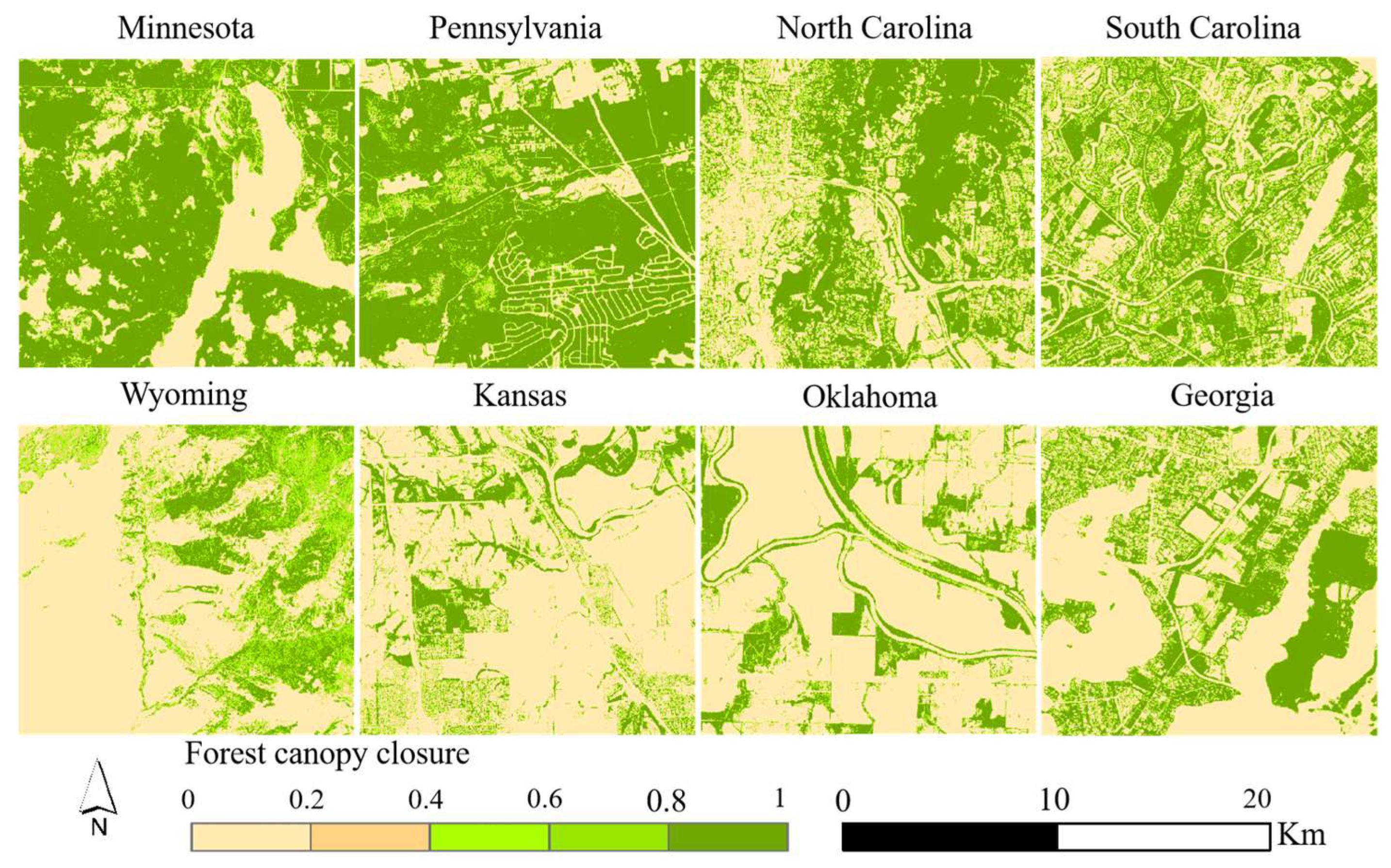
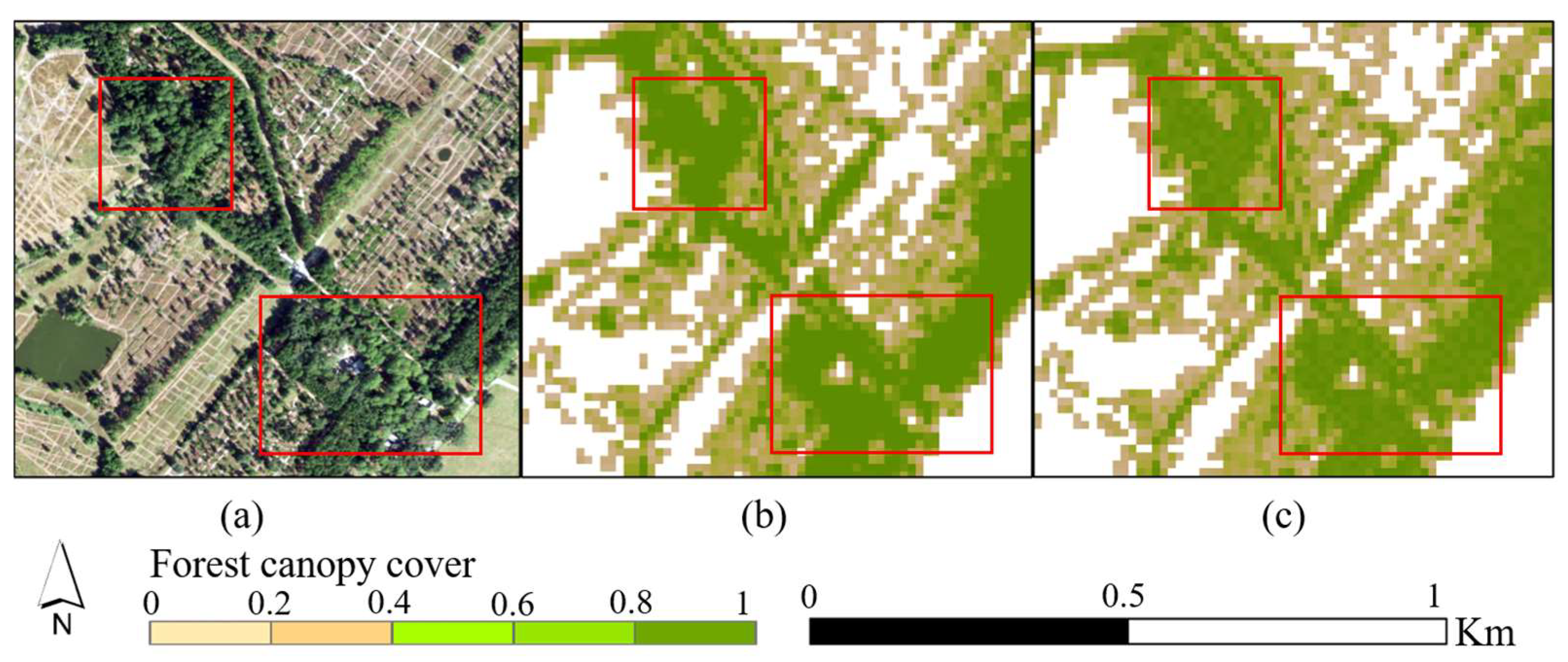
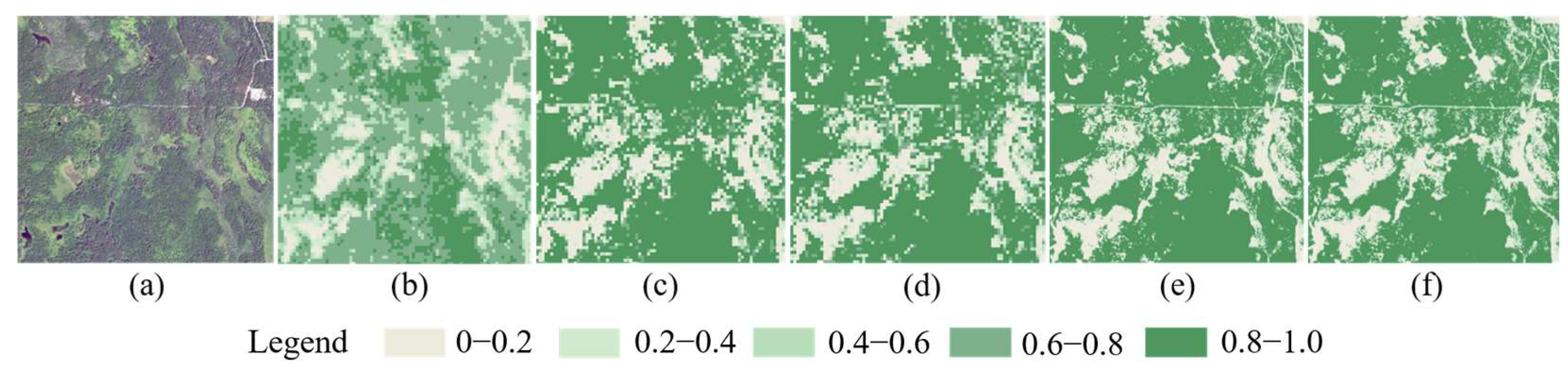
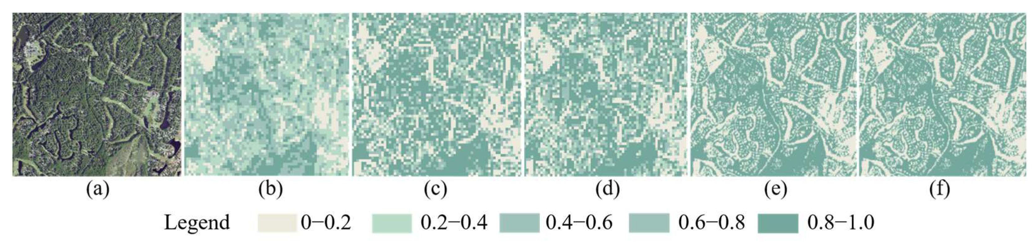
4.4.1. Comparison on Spatial Scale

This study conducted an in-depth analysis of the validation and comparison of forest canopy closure estimation results across different spatial scales. To verify the accuracy of the results, four representative sample plots were selected, located in GA, KS, MN, and OK, each characterized by distinct geographical and climatic conditions. This selection provides a solid basis for assessing the applicability of the estimation results in varied environments. Multiple datasets with different resolutions were utilized, including 0.6 m NAIP aerial imagery, 30 m NLCD TCC, 10 m True TCC, 10 m Model TCC, as well as 30 m True FCC and 30 m Model FCC obtained through resampling.

Using 0.6 m NAIP aerial imagery, high-precision canopy information was obtained, providing reliable reference data for visual interpretation on a small scale. Through visual comparisons of canopy closure data across multiple resolutions for each sample plot, this study assesses the differences between datasets of varying resolutions. As shown in Figure 14, GA, a densely built urban area, displays a dispersed tree arrangement interspersed among residential zones. At the same 30 m resolution, the Model TCC is closer to the actual canopy closure than the NLCD TCC product. In Figure 15, KS, also an urban area, shows a more concentrated tree distribution compared to GA, with the 10 m Model TCC imagery aligning more closely with true canopy closure values. Figure 16 depicts the MN plot, where trees cluster densely; the 30 m Model TCC image reveals grassy gaps between trees, a detail not captured in NLCD TCC. In Figure 17, the OK plot, another densely vegetated area, shows more detailed information in the 10 m Model TCC image compared to the 30 m resolution.

To quantify the accuracy of Model TCC compared with NLCD TCC, this study calculated R², RMSE, MAE, and bias for each study area. As shown in

Table 4. Validation results of Model TCC and NLCD TCC products against True TCC data across four study areas.

Study Area	Data	10 m Tree Canopy Closure Data (True TCC)
		R2	RMSE	MAE	Bias
GA	NLCD TCC	0.59	0.43	9.50%	−7.7%
	Model FCC	0.87	0.16	6.47%	0.47%
KS	NLCD TCC	0.64	0.35	13.50%	−6.97%
	Model FCC	0.81	0.18	11.41%	2.85%
MN	NLCD TCC	0.37	0.47	8.58%	−9.67%
	Model FCC	0.85	0.13	5.08%	2.67%
OK	NLCD TCC	0.68	0.26	23.33%	−14.21%
	Model FCC	0.89	0.10	19.72%	0.07%

, the comparison between the 30 m NLCD TCC product and the 10 m true canopy closure shows a relatively high R² range of 0.37 to 0.68, indicating a strong correlation. However, RMSE and MAE values reveal errors at finer levels, with RMSE reaching 0.43 in GA and 0.47 in MN, while MAE reaches as high as 23.33% in OK. Bias analysis further highlights systematic errors, suggesting that NLCD TCC may underestimate or overestimate canopy closure in certain areas. Similarly, for comparisons between the 10 m Model TCC estimates and the 10 m true canopy closure, R² values are generally higher than those of NLCD TCC, ranging from 0.81 to 0.89, indicating that the XGBoost model’s estimates provide a significant advantage in capturing details and complexity. However, RMSE and MAE values also reveal model errors in some areas, especially in the OK area with its dramatic canopy density variation, where MAE reaches 19.27%. Bias analysis indicates some systematic deviations within the model, but overall, the model estimates show high concordance with the true data.

Through multiscale visual comparisons and statistical analyses, this study provides a comprehensive understanding of the performance and error characteristics of estimation results across different spatial scales. Specifically, 0.6 m NAIP imagery offers the most detailed surface cover information but is challenging for large-scale applications due to its data volume and processing complexity. Although the 30 m NLCD TCC product has a lower resolution, it remains relatively stable for large-scale ecological research. Meanwhile, the 10 m model inversion results demonstrate significant advantages in detail and accuracy, especially for studies and applications requiring high-precision canopy closure data.

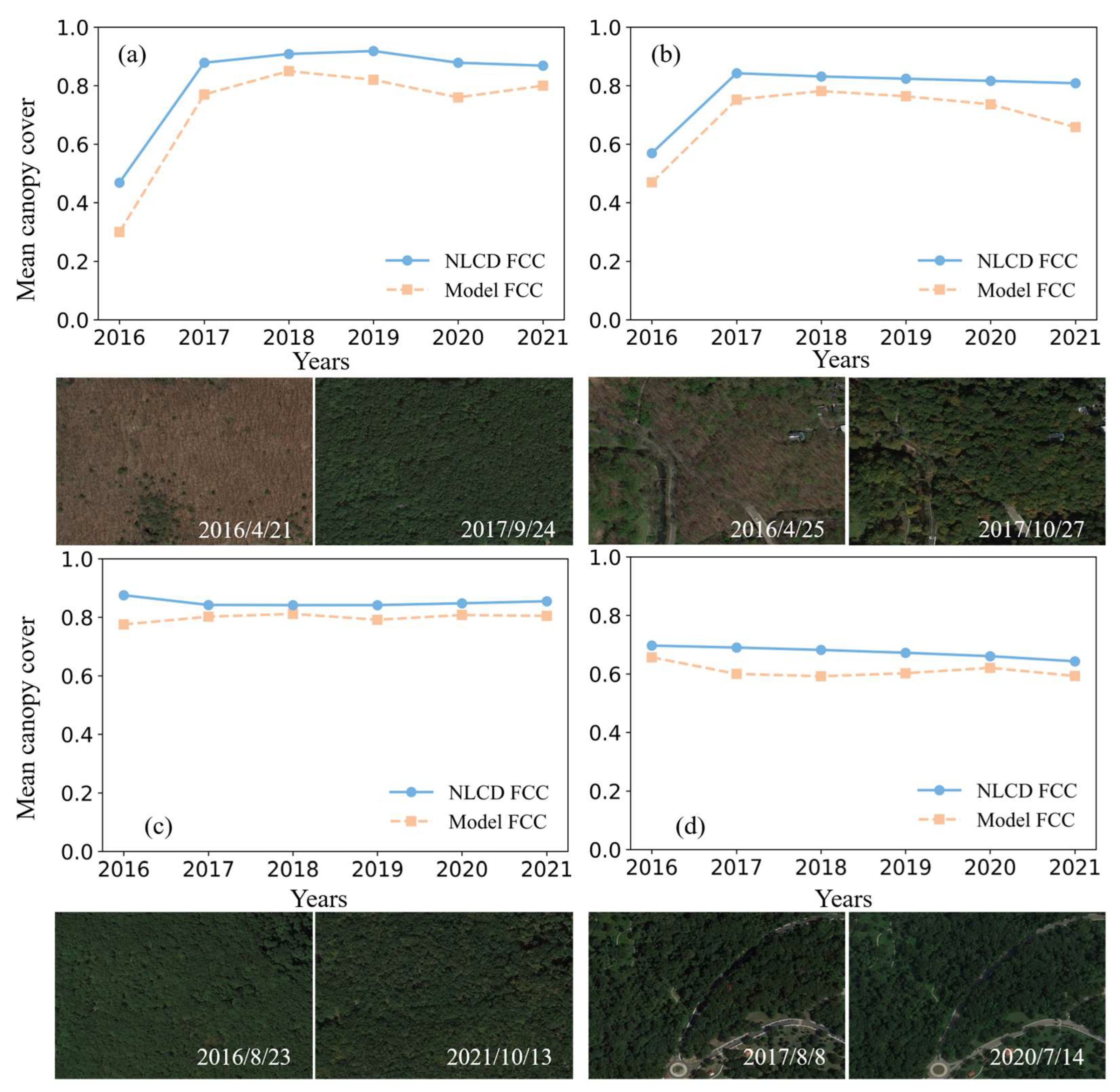
4.4.2. Comparison on Temporal Scale

This study also performed a temporal-scale comparison of the tree canopy closure estimation results. The 10 m model TCC from 2016 to 2021 was resampled to 30 m and compared with the 30 m NLCD TCC for the corresponding plots in June of the same period. The analysis examined the differences in performance between the two datasets both within each year and across multiple years, assessing the model’s stability and accuracy over time.

The comparison between Model TCC and NLCD TCC from 2016 to 2021 across the four study areas (GA, KS, MN, OK) is illustrated in Figure 18: In the GA study area, the average canopy closure trends of Model TCC and NLCD TCC are largely consistent. Notably, there is a significant increase in canopy closure between 2016 and 2017. Google imagery reveals that in April 2016, the area was in a period of tree dormancy, while by September 2017, the trees had become lush and entered a mature phase. This change may reflect specific ecological or management events in the area, such as forest fires, logging activities, or extreme weather impacting canopy closure. From 2017 onward, the canopy closure stabilized, with consistent trends across different years, indicating the reliability of the model inversion in this region. In the KS study area, the overall trends of Model TCC and NLCD TCC are also consistent. Between 2016 and 2017, there is a marked increase in canopy closure. Google imagery shows that the region was in a period of dormancy in April 2016 but reached maturity by October 2017. This change could be attributed to the large climatic variability in Kansas, especially in years prone to droughts and floods, which cause significant fluctuations in canopy closure. However, from 2020 to 2021, the decrease in canopy closure in the model inversion results is noticeably smaller than that observed in the NLCD product, indicating some deviation. In the MN and OK study areas, the mean canopy closure values of Model TCC and NLCD TCC align closely, demonstrating high credibility. In the MN area, the annual average canopy closure is approximately 0.8, with Google imagery showing dense tree canopy coverage. In the OK area, the annual average canopy closure is around 0.7, and compared to the MN area, the canopy appears more sparse in Google imagery. In the time series plots of the four sample areas, the variations in canopy closure between different years and the interannual trends are clearly visible. These plots provide an intuitive comparison of the 30 m Model TCC and 30 m NLCD TCC across different years. Despite some discrepancies in specific years and sample areas, the overall trends indicate a high degree of temporal consistency between the two data sources.

Overall, through the analysis of time series graphs from 2016 to 2021 for the four study areas (GA, KS, MN, and OK), we observed a high degree of consistency between the 10 m Model TCC and the 30 m NLCD TCC in terms of temporal variation trends. This indicates that the 10 m Model TCC can accurately capture forest canopy closure changes over different time scales, providing crucial data support and methodological reference for future forest management and ecological research. Future studies could expand the range of study areas and incorporate longer time series data to comprehensively validate and improve methods for estimating tree canopy closure.

5. Discussion

5.1. Application of Deep Learning in Canopy Closure Estimation

The research combines the U-Net image segmentation model with the Faster R-CNN object detection algorithm to extract tree canopy information from NAIP aerial imagery, as depicted in Figure 4. In this framework, the U-Net image segmentation approach plays a critical role. Specifically, U-Net accurately segments tree canopy regions from high-resolution aerial images, producing high-quality canopy boundary masks. Its distinctive encoder–decoder architecture allows it to effectively capture fine-grained canopy features, including edges, shapes, and textures [75,76]. Moreover, it exhibits robust performance in managing complex backgrounds, including mixed vegetation and terrain variations, effectively mitigating noise interference and improving the accuracy of segmentation [77,78]. Building upon the tree canopy bounding boxes generated by Faster R-CNN, U-Net conducts refined segmentation, significantly improving the accuracy of tree canopy information extraction and enabling a comprehensive workflow from coarse to fine granularity. The exceptional performance of Model TCC in estimating tree canopy closure primarily stems from its algorithmic strengths and its effective integration of multi-source data. By leveraging an ensemble of decision trees, XGBoost adeptly models complex nonlinear relationships involving terrain variability, vegetation diversity, and illumination conditions. Furthermore, its built-in regularization techniques (L1 and L2) mitigate overfitting risks and enhance the model’s generalization performance [79,80]. Additionally, XGBoost can autonomously assess the feature importance of multi-source remote sensing data, such as Sentinel-2 optical imagery, Sentinel-1 radar data, vegetation indices, and land use classification. By effectively exploiting the complementary characteristics of these datasets, it significantly improves estimation accuracy [81]. Deep learning exhibits considerable potential in tree canopy closure estimation. The high precision and detail-capturing capabilities of U-Net, combined with the robustness and efficiency of XGBoost, provide technical support for accurate tree canopy closure mapping. However, future research should further explore the optimization of such methods to enhance their applicability across diverse environments and large-scale regions. For instance, improving generalization across different vegetation types, optimizing computational efficiency, and adapting to larger-scale remote sensing data remain critical areas for further investigation.

5.2. Multi-Source Remote Sensing Data Fusion

Sentinel-2 data deliver high-resolution spectral information, enabling the detection of fine-scale vegetation features and providing a robust spectral basis for the model. Meanwhile, Sentinel-1 data enhance the model’s capability to interpret topographically complex regions, such as mountainous and forested areas, through its radar bands. This is particularly advantageous under cloud cover or suboptimal lighting conditions, effectively addressing the limitations of optical imagery. Furthermore, vegetation indices offer a quantitative measure of vegetation health and coverage density, with prior research underscoring their importance in forest canopy closure estimation [82,83,84]. Simultaneously, land use classification data provide the model with pixel-level land use type information, further strengthening its contextual perception capabilities. As illustrated in Figure 9, the XGBoost model achieves an accuracy of 0.70 when using Sentinel-2 data alone. While this result demonstrates reasonable reliability, it still exhibits limitations in complex terrain and vegetation scenarios. Nevertheless, by integrating Sentinel-1 data, vegetation indices, and land use classification data, the model’s accuracy is significantly enhanced to 0.88. This enhancement not only confirms the efficacy of multi-source data fusion but also highlights that, in complex environments, relying on a single data source may fail to fully capture surface characteristics. In contrast, the integration of multi-source data can substantially improve the accuracy and robustness of tree canopy cover estimation [85,86].

5.3. Limitations and Uncertainties

Despite the notable achievements of this study, several limitations and uncertainties need to be addressed. First, the dependence of U-Net image segmentation on high-resolution aerial imagery presents significant challenges for large-scale applications. Although U-Net can deliver high-precision tree canopy information extraction, the substantial costs and computational complexity involved in acquiring and processing high-resolution data constrain its scalability [87]. To mitigate this issue, future studies could investigate the integration of high-resolution aerial imagery with medium- and low-resolution satellite data (e.g., Sentinel-2, Landsat) to lower costs and improve the feasibility of large-scale monitoring. Secondly, the four models demonstrate inconsistent performance in high-density and low-density regions, highlighting the influence of imbalanced training data distribution on model outcomes. As illustrated in Figure 8, all models exhibit a tendency to underestimate in high-density areas and overestimate in low-density areas, largely attributable to the stratified sampling approach, which results in an overrepresentation of high-density samples and an underrepresentation of low-density samples. This imbalance leads to robust model performance in high-density regions but weaker performance in low-density regions. Specifically, the SVM model fails to identify key features during feature selection, leading to inadequate and non-representative input features. Combined with disparities in sample sizes and label imbalances in the validation set, this further amplifies model bias [88]. In comparison, XGBoost and LightGBM excel in well-balanced datasets, offering high predictive accuracy and stability, but their performance is less optimal in small-scale or unevenly distributed datasets [89]. To mitigate these challenges, future studies could utilize data augmentation techniques (e.g., SMOTE) or resampling approaches to improve data distribution and strengthen the models’ generalization performance.

The integration of multi-source remote sensing data also faces several challenges. For example, variations in resolution, temporal consistency, and spatial coverage across different data sources impose higher requirements for data preprocessing and fusion algorithms. Consequently, future research should further explore the influence of diverse remote sensing data on model accuracy and refine data fusion strategies to enhance the model’s generalization ability and reliability in real-world applications. For instance, advanced feature selection methods and fusion algorithms could be introduced, or deep learning techniques could be incorporated to optimize the effectiveness of multi-source data fusion [90,91]. Multi-source data fusion has exhibited considerable potential in enhancing the accuracy of canopy cover estimation. Nonetheless, its application necessitates further refinement and broader implementation to meet the multifaceted requirements posed by complex environmental conditions. Moreover, existing models are predominantly tailored for small-scale canopy closure assessments and exhibit constrained efficacy in managing spatial heterogeneity [92,93]. To improve the applicability of these methods across extensive areas, future studies should focus on several key directions. One promising approach is the adoption of multi-scale analytical techniques, which synergize high-resolution imagery with medium- and low-resolution satellite data to effectively delineate canopy features at diverse spatial scales [94]. Furthermore, the development of regionally adaptive algorithms, including domain adaptation techniques derived from transfer learning, could be pursued to enable models to effectively accommodate diverse geographical and climatic conditions [95]. These advancements are expected to significantly bolster the model’s proficiency in managing spatial heterogeneity, thereby facilitating its broader implementation in large-scale canopy closure estimation endeavors.

6. Conclusions

This study introduces an advanced methodology aimed at improving the precision of forest canopy closure estimation, culminating in the generation of a high-accuracy 10 m resolution canopy closure product. The results indicate that conventional methods suffer from reduced inversion accuracy due to the impacts of climatic conditions, geographic locations, and complex backgrounds. In contrast, the U-Net-based image segmentation approach for canopy closure estimation demonstrates marked superiority. This innovative method offers an efficient and economical solution for monitoring canopy closure at a regional scale, effectively bridging the gaps associated with traditional ground-based surveys and costly remote sensing techniques in extensive applications. By leveraging high-resolution imagery in conjunction with multi-source remote sensing data, the research not only achieves a notable enhancement in estimation accuracy but also minimizes the expenses related to data acquisition and processing. This advancement provides substantial technical support for forest resource management, biodiversity preservation, and the maintenance of ecological equilibrium, while also contributing methodological insights to ecological monitoring and climate change studies.

References

1. Anderegg, W.R.L.; Trugman, A.T.; Badgley, G.; Anderson, C.M.; Bartuska, A.; Ciais, P.; Cullenward, D.; Field, C.B.; Freeman, J.; Goetz, S.J.; et al. Climate-driven risks to the climate mitigation potential of forests. Science 2020, 368, eaaz7005. [Google Scholar] [CrossRef] [PubMed]
2. Goldstein, A.; Turner, W.R.; Spawn, S.A.; Anderson-Teixeira, K.J.; Cook-Patton, S.; Fargione, J.; Gibbs, H.K.; Griscom, B.; Hewson, J.H.; Howard, J.F.; et al. Protecting irrecoverable carbon in Earth’s ecosystems. Nat. Clim. Change 2020, 10, 287–295. [Google Scholar] [CrossRef]
3. Rustad, L.E. The response of terrestrial ecosystems to global climate change: Towards an integrated approach. Sci. Total Environ. 2008, 404, 222–235. [Google Scholar] [CrossRef] [PubMed]
4. Watson, J.E.M.; Evans, T.; Venter, O.; Williams, B.; Tulloch, A.; Stewart, C.; Thompson, I.; Ray, J.C.; Murray, K.; Salazar, A.; et al. The exceptional value of intact forest ecosystems. Nat. Ecol. Evol. 2018, 2, 599–610. [Google Scholar] [CrossRef]
5. Zhang, L.; Sun, P.S.; Huettmann, F.; Liu, S.R. Where should China practice forestry in a warming world? Glob. Change Biol. 2022, 28, 2461–2475. [Google Scholar] [CrossRef]
6. Cai, W.X.; He, N.P.; Li, M.X.; Xu, L.; Wang, L.Z.; Zhu, J.H.; Zeng, N.; Yan, P.; Si, G.X.; Zhang, X.Q.; et al. Carbon sequestration of Chinese forests from 2010 to 2060 spatiotemporal dynamics and its regulatory strategies. Sci. Bull. 2022, 67, 836–843. [Google Scholar] [CrossRef]
7. Cao, S.X.; Lu, C.X.; Yue, H. Optimal Tree Canopy Cover during Ecological Restoration: A Case Study of Possible Ecological Thresholds in Changting, China. Bioscience 2017, 67, 221–232. [Google Scholar] [CrossRef]
8. Nakamura, A.; Kitching, R.L.; Cao, M.; Creedy, T.J.; Fayle, T.M.; Freiberg, M.; Hewitt, C.N.; Itioka, T.; Koh, L.P.; Ma, K.; et al. Forests and Their Canopies: Achievements and Horizons in Canopy Science. Trends Ecol. Evol. 2017, 32, 438–451. [Google Scholar] [CrossRef]
9. Zomer, R.J.; Bossio, D.A.; Trabucco, A.; van Noordwijk, M.; Xu, J. Global carbon sequestration potential of agroforestry and increased tree cover on agricultural land. Circ. Agric. Syst. 2022, 2, 1–10. [Google Scholar] [CrossRef]
10. Taneja, R.; Wallace, L.; Reinke, K.; Hilton, J.; Jones, S. Differences in Canopy Cover Estimations from ALS Data and Their Effect on Fire Prediction. Environ. Model. Assess. 2023, 28, 565–583. [Google Scholar] [CrossRef]
11. Büchi, L.; Wendling, M.; Mouly, P.; Charles, R. Comparison of Visual Assessment and Digital Image Analysis for Canopy Cover Estimation. Agron. J. 2018, 110, 1289–1295. [Google Scholar] [CrossRef]
12. Martin, D.A.; Wurz, A.; Osen, K.; Grass, I.; Hölscher, D.; Rabemanantsoa, T.; Tscharntke, T.; Kreft, H. Shade-Tree Rehabilitation in Vanilla Agroforests is Yield Neutral and May Translate into Landscape-Scale Canopy Cover Gains. Ecosystems 2021, 24, 1253–1267. [Google Scholar] [CrossRef]
13. Tang, H.; Armston, J.; Hancock, S.; Marselis, S.; Goetz, S.; Dubayah, R. Characterizing global forest canopy cover distribution using spaceborne lidar. Remote Sens. Environ. 2019, 231, 11. [Google Scholar] [CrossRef]
14. Bonney, M.T.; He, Y.H.; Vogeler, J.; Conway, T.; Kaye, E. Mapping canopy cover for municipal forestry monitoring: Using free Landsat imagery and machine learning. Urban For. Urban Green. 2024, 100, 18. [Google Scholar] [CrossRef]
15. Wang, X.J.; Scott, C.E.; Dallimer, M. High summer land surface temperatures in a temperate city are mitigated by tree canopy cover. Urban CLim. 2023, 51, 11. [Google Scholar] [CrossRef]
16. Qiu, Z.X.; Feng, Z.K.; Song, Y.N.; Li, M.L.; Zhang, P.P. Carbon sequestration potential of forest vegetation in China from 2003 to 2050: Predicting forest vegetation growth based on climate and the environment. J. Clean. Prod. 2020, 252, 14. [Google Scholar] [CrossRef]
17. Zhang, Y.; Yuan, J.; You, C.M.; Cao, R.; Tan, B.; Li, H.; Yang, W.Q. Contributions of National Key Forestry Ecology Projects to the forest vegetation carbon storage in China. For. Ecol. Manag. 2020, 462, 8. [Google Scholar] [CrossRef]
18. Li, Z.; Ota, T.; Mizoue, N. Monitoring tropical forest change using tree canopy cover time series obtained from Sentinel-1 and Sentinel-2 data. Int. J. Digit. Earth 2024, 17, 17. [Google Scholar] [CrossRef]
19. Schleeweis, K.; Goward, S.N.; Huang, C.Q.; Masek, J.G.; Moisen, G.; Kennedy, R.E.; Thomas, N.E. Regional dynamics of forest canopy change and underlying causal processes in the contiguous US. J. Geophys. Res.-Biogeosci. 2013, 118, 1035–1053. [Google Scholar] [CrossRef]
20. Dash, J.P.; Watt, M.S.; Pearse, G.D.; Heaphy, M.; Dungey, H.S. Assessing very high resolution UAV imagery for monitoring forest health during a simulated disease outbreak. ISPRS-J. Photogramm. Remote Sens. 2017, 131, 1–14. [Google Scholar] [CrossRef]
21. Ulmer, J.M.; Wolf, K.L.; Backman, D.R.; Tretheway, R.L.; Blain, C.J.A.; O’Neil-Dunne, J.P.M.; Frank, L.D. Multiple health benefits of urban tree canopy: The mounting evidence for a green prescription. Health Place 2016, 42, 54–62. [Google Scholar] [CrossRef] [PubMed]
22. De Lombaerde, E.; Vangansbeke, P.; Lenoir, J.; Van Meerbeek, K.; Lembrechts, J.; Rodríguez-Sánchez, F.; Luoto, M.; Scheffers, B.; Haesen, S.; Aalto, J.; et al. Maintaining forest cover to enhance temperature buffering under future climate change. Sci. Total Environ. 2022, 810, 9. [Google Scholar] [CrossRef]
23. Halpern, C.B.; Lutz, J.A. Canopy closure exerts weak controls on understory dynamics: A 30-year study of overstory-understory interactions. Ecol. Monogr. 2013, 83, 221–237. [Google Scholar] [CrossRef]
24. Parent, J.R.; Volin, J.C. Assessing the potential for leaf-off LiDAR data to model canopy closure in temperate deciduous forests. ISPRS-J. Photogramm. Remote Sens. 2014, 95, 134–145. [Google Scholar] [CrossRef]
25. Paletto, A.; Tosi, V. Forest canopy cover and canopy closure: Comparison of assessment techniques. Eur. J. For. Res. 2009, 128, 265–272. [Google Scholar] [CrossRef]
26. Gyawali, A.; Aalto, M.; Peuhkurinen, J.; Villikka, M.; Ranta, T. Comparison of Individual Tree Height Estimated from LiDAR and Digital Aerial Photogrammetry in Young Forests. Sustainability 2022, 14, 3720. [Google Scholar] [CrossRef]
27. Gonçalves, F.; Treuhaft, R.; Law, B.; Almeida, A.; Walker, W.; Baccini, A.; dos Santos, J.R.; Graça, P. Estimating Aboveground Biomass in Tropical Forests: Field Methods and Error Analysis for the Calibration of Remote Sensing Observations. Remote Sens. 2017, 9, 47. [Google Scholar] [CrossRef]
28. Ganz, S.; Käber, Y.; Adler, P. Measuring Tree Height with Remote Sensing-A Comparison of Photogrammetric and LiDAR Data with Different Field Measurements. Forests 2019, 10, 694. [Google Scholar] [CrossRef]
29. Gonzalez, P.; Asner, G.P.; Battles, J.J.; Lefsky, M.A.; Waring, K.M.; Palace, M. Forest carbon densities and uncertainties from Lidar, QuickBird, and field measurements in California. Remote Sens. Environ. 2010, 114, 1561–1575. [Google Scholar] [CrossRef]
30. Fleck, S.; Mölder, I.; Jacob, M.; Gebauer, T.; Jungkunst, H.F.; Leuschner, C. Comparison of conventional eight-point crown projections with LIDAR-based virtual crown projections in a temperate old-growth forest. Ann. For. Sci. 2011, 68, 1173–1185. [Google Scholar] [CrossRef]
31. Atkins, J.W.; Bhatt, P.; Carrasco, L.; Francis, E.; Garabedian, J.E.; Hakkenberg, C.R.; Hardiman, B.S.; Jung, J.H.; Koirala, A.; Larue, E.A.; et al. Integrating forest structural diversity measurement into ecological research. Ecosphere 2023, 14, 17. [Google Scholar] [CrossRef]
32. Jurjevic, L.; Liang, X.L.; Gasparovic, M.; Balenovic, I. Is field-measured tree height as reliable as believed—Part II, A comparison study of tree height estimates from conventional field measurement and low-cost close-range remote sensing in a deciduous forest. ISPRS-J. Photogramm. Remote Sens. 2020, 169, 227–241. [Google Scholar] [CrossRef]
33. Unger, D.R.; Hung, I.K.; Brooks, R.; Williams, H. Estimating number of trees, tree height and crown width using Lidar data. GISci. Remote Sens. 2014, 51, 227–238. [Google Scholar] [CrossRef]
34. Ma, Q.; Su, Y.J.; Guo, Q.H. Comparison of Canopy Cover Estimations From Airborne LiDAR, Aerial Imagery, and Satellite Imagery. IEEE J. Sel. Top. Appl. Earth Observ. Remote Sens. 2017, 10, 4225–4236. [Google Scholar] [CrossRef]
35. McIntosh, A.C.S.; Gray, A.N.; Garman, S.L. Estimating Canopy Cover from Standard Forest Inventory Measurements in Western Oregon. For. Sci. 2012, 58, 154–167. [Google Scholar] [CrossRef]
36. Ucar, Z.; Bettinger, P.; Merry, K.; Siry, J.; Bowker, J.M.; Akbulut, R. A comparison of two sampling approaches for assessing the urban forest canopy cover from aerial photography. Urban For. Urban Green. 2016, 16, 221–230. [Google Scholar] [CrossRef]
37. Joshi, C.; De Leeuw, J.; Skidmore, A.K.; van Duren, I.C.; van Oosten, H. Remotely sensed estimation of forest canopy density: A comparison of the performance of four methods. Int. J. Appl. Earth Obs. Geoinf. 2006, 8, 84–95. [Google Scholar] [CrossRef]
38. Zhu, Y.Y.; Jeon, S.; Sung, H.; Kim, Y.; Park, C.; Cha, S.; Jo, H.W.; Lee, W.K. Developing UAV-Based Forest Spatial Information and Evaluation Technology for Efficient Forest Management. Sustainability 2020, 12, 10150. [Google Scholar] [CrossRef]
39. Michez, A.; Huylenbroeck, L.; Bolyn, C.; Latte, N.; Bauwens, S.; Lejeune, P. Can regional aerial images from orthophoto surveys produce high quality photogrammetric Canopy Height Model? A single tree approach in Western Europe. Int. J. Appl. Earth Obs. Geoinf. 2020, 92, 10. [Google Scholar] [CrossRef]
40. Corona, P.; Chirici, G.; Franceschi, S.; Maffei, D.; Marcheselli, M.; Pisani, C.; Fattorini, L. Design-based treatment of missing data in forest inventories using canopy heights from aerial laser scanning. Can. J. For. Res. 2014, 44, 892–902. [Google Scholar] [CrossRef]
41. Kangas, A.; Astrup, R.; Breidenbach, J.; Fridman, J.; Gobakken, T.; Korhonen, K.T.; Maltamo, M.; Nilsson, M.; Nord-Larsen, T.; Næsset, E.; et al. Remote sensing and forest inventories in Nordic countries—Roadmap for the future. Scand. J. For. Res. 2018, 33, 397–412. [Google Scholar] [CrossRef]
42. Lefsky, M.A.; Cohen, W.B.; Parker, G.G.; Harding, D.J. Lidar remote sensing for ecosystem studies: Lidar, an emerging remote sensing technology that directly measures the three-dimensional distribution of plant canopies, can accurately estimate vegetation structural attributes and should be of particular interest to forest, landscape, and global ecologists. Bioscience 2002, 52, 19–30. [Google Scholar]
43. Zhao, K.G.; Popescu, S.; Meng, X.L.; Pang, Y.; Agca, M. Characterizing forest canopy structure with lidar composite metrics and machine learning. Remote Sens. Environ. 2011, 115, 1978–1996. [Google Scholar] [CrossRef]
44. Brandt, J.; Ertel, J.; Spore, J.; Stolle, F. Wall-to-wall mapping of tree extent in the tropics with Sentinel-1 and Sentinel-2. Remote Sens. Environ. 2023, 292, 19. [Google Scholar] [CrossRef]
45. Nasiri, V.; Darvishsefat, A.A.; Arefi, H.; Griess, V.C.; Sadeghi, S.M.M.; Borz, S.A. Modeling Forest Canopy Cover: A Synergistic Use of Sentinel-2, Aerial Photogrammetry Data, and Machine Learning. Remote Sens. 2022, 14, 1453. [Google Scholar] [CrossRef]
46. Silveira, E.M.O.; Radeloff, V.C.; Martinuzzi, S.; Pastur, G.J.M.; Bono, J.; Politi, N.; Lizarraga, L.; Rivera, L.O.; Ciuffoli, L.; Rosas, Y.M.; et al. Nationwide native forest structure maps for Argentina based on forest inventory data, SAR Sentinel-1 and vegetation metrics from Sentinel-2 imagery. Remote Sens. Environ. 2023, 285, 17. [Google Scholar] [CrossRef]
47. Heckel, K.; Urban, M.; Schratz, P.; Mahecha, M.D.; Schmullius, C. Predicting Forest Cover in Distinct Ecosystems: The Potential of Multi-Source Sentinel-1 and-2 Data Fusion. Remote Sens. 2020, 12, 302. [Google Scholar] [CrossRef]
48. Li, W.; Niu, Z.; Shang, R.; Qin, Y.C.; Wang, L.; Chen, H.Y. High-resolution mapping of forest canopy height using machine learning by coupling ICESat-2 LiDAR with Sentinel-1, Sentinel-2 and Landsat-8 data. Int. J. Appl. Earth Obs. Geoinf. 2020, 92, 14. [Google Scholar] [CrossRef]
49. Tang, X.; Bratley, K.H.; Cho, K.; Bullock, E.L.; Olofsson, P.; Woodcock, C.E. Near real-time monitoring of tropical forest disturbance by fusion of Landsat, Sentinel-2, and Sentinel-1 data. Remote Sens. Environ. 2023, 294, 113626. [Google Scholar] [CrossRef]
50. Waldeland, A.U.; Trier, O.D.; Salberg, A.B. Forest mapping and monitoring in Africa using Sentinel-2 data and deep learning. Int. J. Appl. Earth Obs. Geoinf. 2022, 111, 13. [Google Scholar] [CrossRef]
51. Fiore, N.M.; Goulden, M.L.; Czimczik, C.I.; Pedron, S.A.; Tayo, M.A. Do recent NDVI trends demonstrate boreal forest decline in Alaska? Environ. Res. Lett. 2020, 15, 095007. [Google Scholar] [CrossRef]
52. Abrams, J.F.; Vashishtha, A.; Wong, S.T.; Nguyen, A.; Mohamed, A.; Wieser, S.; Kuijper, A.; Wilting, A.; Mukhopadhyay, A. Habitat-Net: Segmentation of habitat images using deep learning. Ecol. Inform. 2019, 51, 121–128. [Google Scholar] [CrossRef]
53. Niedballa, J.; Axtner, J.; Döbert, T.F.; Tilker, A.; Nguyen, A.; Wong, S.T.; Fiderer, C.; Heurich, M.; Wilting, A. imageseg: An R package for deep learning-based image segmentation. Methods Ecol. Evol. 2022, 13, 2363–2371. [Google Scholar] [CrossRef]
54. Vicente-Serrano, S.M.; Camarero, J.J.; Olano, J.M.; Martín-Hernández, N.; Peña-Gallardo, M.; Tomás-Burguera, M.; Gazol, A.; Azorin-Molina, C.; Bhuyan, U.; El Kenawy, A. Diverse relationships between forest growth and the Normalized Difference Vegetation Index at a global scale. Remote Sens. Environ. 2016, 187, 14–29. [Google Scholar] [CrossRef]
55. Yang, Q.L.; Zhang, H.; Peng, W.S.; Lan, Y.Y.; Luo, S.S.; Shao, J.M.; Chen, D.Z.; Wang, G.Q. Assessing climate impact on forest cover in areas undergoing substantial land cover change using Landsat imagery. Sci. Total Environ. 2019, 659, 732–745. [Google Scholar] [CrossRef]
56. Krishnan, S.; Pradhan, A.; Indu, J. Estimation of high-resolution precipitation using downscaled satellite soil moisture and SM2RAIN approach. J. Hydrol. 2022, 610, 14. [Google Scholar] [CrossRef]
57. Phompila, C.; Lewis, M.; Ostendorf, B.; Clarke, K. MODIS EVI and LST Temporal Response for Discrimination of Tropical Land Covers. Remote Sens. 2015, 7, 6026–6040. [Google Scholar] [CrossRef]
58. Huang, C.Y.; Durán, S.M.; Hu, K.T.; Li, H.J.; Swenson, N.G.; Enquist, B.J. Remotely sensed assessment of increasing chronic and episodic drought effects on a Costa Rican tropical dry forest. Ecosphere 2021, 12, 19. [Google Scholar] [CrossRef]
59. Wang, L.L.; Hunt, E.R.; Qu, J.J.; Hao, X.J.; Daughtry, C.S.T. Towards estimation of canopy foliar biomass with spectral reflectance measurements. Remote Sens. Environ. 2011, 115, 836–840. [Google Scholar] [CrossRef]
60. Danson, F.M.; Hetherington, D.; Morsdorf, F.; Koetz, B.; Allgöwer, B. Forest canopy gap fraction from terrestrial laser scanning. IEEE Geosci. Remote Sens. Lett. 2007, 4, 157–160. [Google Scholar] [CrossRef]
61. Gonsamo, A. Leaf area index retrieval using gap fractions obtained from high resolution satellite data: Comparisons of approaches, scales and atmospheric effects. Int. J. Appl. Earth Obs. Geoinf. 2010, 12, 233–248. [Google Scholar] [CrossRef]
62. Chen, A.; Orlov-Levin, V.; Meron, M. Applying high-resolution visible-channel aerial imaging of crop canopy to precision irrigation management. Agric. Water Manag. 2019, 216, 196–205. [Google Scholar] [CrossRef]
63. Su, Y.J.; Guo, Q.H.; Ma, Q.; Li, W.K. SRTM DEM Correction in Vegetated Mountain Areas through the Integration of Spaceborne LiDAR, Airborne LiDAR, and Optical Imagery. Remote Sens. 2015, 7, 11202–11225. [Google Scholar] [CrossRef]
64. Li, H.; Di, L.P.; Zhang, C.; Lin, L.; Guo, L.Y.; Yu, E.G.; Yang, Z.W. Automated In-Season Crop-Type Data Layer Mapping Without Ground Truth for the Conterminous United States Based on Multisource Satellite Imagery. IEEE Trans. Geosci. Remote Sensing 2024, 62, 14. [Google Scholar] [CrossRef]
65. Chaaban, F.; El Khattabi, J.; Darwishe, H. Accuracy Assessment of ESA WorldCover 2020 and ESRI 2020 Land Cover Maps for a Region in Syria. J. Geovis. Spat. Anal. 2022, 6, 23. [Google Scholar] [CrossRef]
66. Freudenberg, M.; Magdon, P.; Nölke, N. Individual tree crown delineation in high-resolution remote sensing images based on U-Net. Neural Comput. Appl. 2022, 34, 22197–22207. [Google Scholar] [CrossRef]
67. Ko, D.; Bristow, N.; Greenwood, D.; Weisberg, P. Canopy Cover Estimation in Semiarid Woodlands: Comparison of Field-Based and Remote Sensing Methods. For. Sci. 2009, 55, 132–141. [Google Scholar] [CrossRef]
68. Ke, C.Y.; He, S.; Qin, Y.G. Comparison of natural breaks method and frequency ratio dividing attribute intervals for landslide susceptibility mapping. Bull. Eng. Geol. Environ. 2023, 82, 18. [Google Scholar] [CrossRef]
69. Ester, M.; Kriegel, H.P.; Xu, X. XGBoost: A scalable tree boosting system. In Proceedings of the 22nd ACM SIGKDD International Conference on Knowledge Discovery and Data Mining, San Francisco, CA, USA, 13–17 August 2016; pp. 785–794. [Google Scholar]
70. Probst, P.; Wright, M.N.; Boulesteix, A.L. Hyperparameters and tuning strategies for random forest. Wiley Interdiscip. Rev.-Data Mining Knowl. Discov. 2019, 9, 15. [Google Scholar]
71. Zhou, Z.G.; Zhao, L.; Lin, A.W.; Qin, W.M.; Lu, Y.B.; Li, J.Y.; Zhong, Y.; He, L.J. Exploring the potential of deep factorization machine and various gradient boosting models in modeling daily reference evapotranspiration in China. Arab. J. Geosci. 2020, 13, 20. [Google Scholar] [CrossRef]
72. Mushava, J.; Murray, M. Flexible loss functions for binary classification in gradient-boosted decision trees: An application to credit scoring. Expert Syst. Appl. 2024, 238, 16. [Google Scholar] [CrossRef]
73. Mo, X.L.; Chen, X.J.; Leong, C.F.; Zhang, S.; Li, H.Y.; Li, J.L.; Lin, G.H.; Sun, G.C.; He, F.; He, Y.L.; et al. Early Prediction of Clinical Response to Etanercept Treatment in Juvenile Idiopathic Arthritis Using Machine Learning. Front. Pharmacol. 2020, 11, 9. [Google Scholar] [CrossRef]
74. Peng, R.T.; Xiao, Z.L.; Peng, Y.H.; Zhang, X.X.; Zhao, L.F.; Gao, J.X. Research on multi-source information fusion tool wear monitoring based on MKW-GPR model. Measurement 2025, 242, 14. [Google Scholar] [CrossRef]
75. Beeche, C.; Singh, J.P.; Leader, J.K.; Gezer, N.S.; Oruwari, A.P.; Dansingani, K.K.; Chhablani, J.; Pu, J.T. Super U-Net: A modularized generalizable architecture. Pattern Recognit. 2022, 128, 12. [Google Scholar] [CrossRef]
76. Li, X.X.; Liu, X.J.; Xiao, Y.; Zhang, Y.; Yang, X.M.; Zhang, W.H. An Improved U-Net Segmentation Model That Integrates a Dual Attention Mechanism and a Residual Network for Transformer Oil Leakage Detection. Energies 2022, 15, 4238. [Google Scholar] [CrossRef]
77. Poonguzhali, R.; Ahmad, S.; Sivasankar, P.T.; Babu, S.A.; Joshi, P.; Joshi, G.P.; Kim, S.W. Automated Brain Tumor Diagnosis Using Deep Residual U-Net Segmentation Model. CMC-Comput. Mat. Contin. 2023, 74, 2179–2194. [Google Scholar]
78. Shwartz-Ziv, R.; Armon, A. Tabular data: Deep learning is not all you need. Inf. Fusion 2022, 81, 84–90. [Google Scholar] [CrossRef]
79. Zhang, J.; Wang, R.R.; Lu, Y.J.; Huang, J.D. Prediction of Compressive Strength of Geopolymer Concrete Landscape Design: Application of the Novel Hybrid RF-GWO-XGBoost Algorithm. Buildings 2024, 14, 591. [Google Scholar] [CrossRef]
80. Tang, M.Z.; Liang, Z.X.; Wu, H.W.; Wang, Z.M. Fault Diagnosis Method for Wind Turbine Gearboxes Based on IWOA-RF. Energies 2021, 14, 6283. [Google Scholar] [CrossRef]
81. Nanko, K.; Giambelluca, T.W.; Sutherland, R.A.; Mudd, R.G.; Nullet, M.A.; Ziegler, A.D. Erosion Potential under Miconia calvescens Stands on the Island of Hawai’i. Land Degrad. Dev. 2015, 26, 218–226. [Google Scholar] [CrossRef]
82. Lin, Y.Y.; Jin, Y.D.; Ge, Y.; Hu, X.S.; Weng, A.F.; Wen, L.S.; Zhou, Y.R.; Li, B.Y. Insights into forest vegetation changes and landscape fragmentation in Southeastern China: From a perspective of spatial coupling and machine learning. Ecol. Indic. 2024, 166, 13. [Google Scholar] [CrossRef]
83. Zhu, W.B.; Zhang, X.D.; Zhang, J.J.; Zhu, L.Q. A comprehensive analysis of phenological changes in forest vegetation of the Funiu Mountains, China. J. Geogr. Sci. 2019, 29, 131–145. [Google Scholar] [CrossRef]
84. Narine, L.; Malambo, L.; Popescu, S. Characterizing canopy cover with ICESat-2: A case study of southern forests in Texas and Alabama, USA. Remote Sens. Environ. 2022, 281, 14. [Google Scholar] [CrossRef]
85. Ashapure, A.; Jung, J.H.; Chang, A.J.; Oh, S.; Maeda, M.; Landivar, J. A Comparative Study of RGB and Multispectral Sensor-Based Cotton Canopy Cover Modelling Using Multi-Temporal UAS Data. Remote Sens. 2019, 11, 2757. [Google Scholar] [CrossRef]
86. Zhou, Q.B.; Yu, Q.Y.; Liu, J.; Wu, W.B.; Tang, H.J. Perspective of Chinese GF-1 high-resolution satellite data in agricultural remote sensing monitoring. J. Integr. Agric. 2017, 16, 242–251. [Google Scholar] [CrossRef]
87. Wu, X.H.; Zuo, W.M.; Lin, L.; Jia, W.; Zhang, D. F-SVM: Combination of Feature Transformation and SVM Learning via Convex Relaxation. IEEE Trans. Neural Netw. Learn. Syst. 2018, 29, 5185–5199. [Google Scholar] [CrossRef]
88. Cai, Y.H.; Feng, J.X.; Wang, Y.Q.; Ding, Y.M.; Hu, Y.; Fang, H. The Optuna-LightGBM-XGBoost Model: A Novel Approach for Estimating Carbon Emissions Based on the Electricity-Carbon Nexus. Appl. Sci. 2024, 14, 4632. [Google Scholar] [CrossRef]
89. Shi, M.Y.; Gao, Y.S.; Chen, L.; Liu, X.Z. Multisource Information Fusion Network for Optical Remote Sensing Image Super-Resolution. IEEE J. Sel. Top. Appl. Earth Observ. Remote Sens. 2023, 16, 3805–3818. [Google Scholar] [CrossRef]
90. Wei, X.L.; Bai, K.X.; Chang, N.B.; Gao, W. Multi-source hierarchical data fusion for high-resolution AOD mapping in a forest fire event. Int. J. Appl. Earth Obs. Geoinf. 2021, 102, 11. [Google Scholar] [CrossRef]
91. Denny, C.K.; Nielsen, S.E. Spatial Heterogeneity of the Forest Canopy Scales with the Heterogeneity of an Understory Shrub Based on Fractal Analysis. Forests 2017, 8, 146. [Google Scholar] [CrossRef]
92. Liu, Y.Y.; Bian, Z.Q.; Ding, S.Y. Consequences of Spatial Heterogeneity of Forest Landscape on Ecosystem Water Conservation Service in the Yi River Watershed in Central China. Sustainability 2020, 12, 1170. [Google Scholar] [CrossRef]
93. Armstrong, A.H.; Huth, A.; Osmanoglu, B.; Sun, G.; Ranson, K.J.; Fischer, R. A multi-scaled analysis of forest structure using individual-based modeling in a costa rican rainforest. Ecol. Model. 2020, 433, 10. [Google Scholar] [CrossRef]
94. Camarero, J.J.; Colangelo, M.; Gazol, A.; Pizarro, M.; Valeriano, C.; Igual, J.M. Effects of Windthrows on Forest Cover, Tree Growth and Soil Characteristics in Drought-Prone Pine Plantations. Forests 2021, 12, 817. [Google Scholar] [CrossRef]
95. Xu, J.L.; Xiao, L.; López, A.M. Self-Supervised Domain Adaptation for Computer Vision Tasks. IEEE Access 2019, 7, 156694–156706. [Google Scholar] [CrossRef]
Figure 1. Schematic diagram of the study area.
Remotesensing 17 01828 g001
Figure 2. Research methods and processes.
Remotesensing 17 01828 g002
Figure 3. Four evaluation metrics for training the U-Net model.
Remotesensing 17 01828 g003
Figure 4. Processing workflow of true tree canopy closure values in the study area, illustrated using a small area in Oklahoma as an example.
Remotesensing 17 01828 g004
Figure 5. The spatial distribution of sampling points within the study area is illustrated using KS, OK, PA, and SC as representative cases.
Remotesensing 17 01828 g005
Figure 6. Crown identification: (a,c,e,g) are small regions of NAIP aerial images in Oklahoma; (b,d,f,h) are corresponding tree canopy distribution maps obtained using Faster R-CNN object detector and U-Net image segmentation techniques.
Remotesensing 17 01828 g006
Figure 7. Importance of feature variables in each model, using recursive feature elimination to select key features from 26 variables in the XGBoost, RF, LightGBM, and SVM models.
Remotesensing 17 01828 g007
Figure 8. The correlation matrix between feature variables and the true values of canopy closure, including the correlations among the 26 feature variables and their respective correlations with the true values of canopy closure.
Remotesensing 17 01828 g008
Figure 9. Validation results of different models: (a) Comparison between the estimation results of 6314 vali dation samples using the RF model and the true values; (b) comparison between the estimation results of 6314 validation samples using the SVM model and the true values; (c) comparison between the estimation results of 6314 validation samples using the XGBoost model and the true values; (d) comparison between the estimation results of 6314 validation samples using the LightGBM model and the true values.
Remotesensing 17 01828 g009
Figure 10. Accuracy improvement of the XGBoost model with progressively added feature variables: The x-axis O represents the initial three features NDVI, SWRI2, and BLUE added to the model; D represents DVI; N represents NDMI; G represents GNDVI; L represents LandCover; V represents VH and VV, added sequentially to the model. (a) Changes in R2 with the sequential addition of feature variables; (b) changes in RMSE with the sequential addition of feature variables; (c) changes in MAE with the sequential addition of feature variables.
Remotesensing 17 01828 g010
Figure 11. The results of canopy closure modeling for the study areas.
Remotesensing 17 01828 g011
Figure 12. The true canopy closure for the study areas.
Remotesensing 17 01828 g012
Figure 13. Local comparison of True TCC and Model TCC. (a) NAIP aerial imagery (b) 10 m True TCC (c) 10 m Model TCC.
Remotesensing 17 01828 g013
Figure 14. Comparison of canopy closure modeling results in Georgia with true canopy closure, NLCD canopy closure products. (a) NAIP aerial imagery; (b) 30 m NLCD TCC product; (c) 30 m True TCC; (d) 30 m Model TCC; (e) 10 m True TCC; (f) 10 m Model TCC.
Remotesensing 17 01828 g014
Figure 15. Comparison of canopy closure modeling results in Kansas with true canopy closure, NLCD canopy closure products. (a) NAIP aerial imagery; (b) 30 m NLCD TCC product; (c) 30 m True TCC; (d) 30 m Model TCC; (e) 10 m True TCC; (f) 10 m Model TCC.
Remotesensing 17 01828 g015
Figure 16. Comparison of canopy closure modeling results in Minnesota with true canopy closure, NLCD canopy closure products. (a) NAIP aerial imagery; (b) 30 m NLCD TCC product; (c) 30 m True TCC; (d) 30 m Model TCC; (e) 10 m True TCC; (f) 10 m Model TCC.
Remotesensing 17 01828 g016
Figure 17. Comparison of canopy closure modeling results in Oklahoma with true canopy closure, NLCD canopy closure products. (a) NAIP aerial imagery; (b) 30 m NLCD TCC product; (c) 30 m True TCC; (d) 30 m Model TCC; (e) 10 m True TCC; (f) 10 m Model TCC.
Remotesensing 17 01828 g017
Figure 18. Compares the Model TCC from 2016 to 2021 with the NLCD TCC: the blue solid line represents the mean canopy cover within the region from the NLCD TCC, and the yellow dashed line represents the model estimation result’s mean canopy cover within the region. (a) Comparison of the mean values of selected small plots in the GA study area; (b) comparison of the mean values of selected small plots in the KS study area; (c) comparison of the mean values of selected small plots in the MN study area; (d) comparison of the mean values of selected small plots in the OK study area.
Remotesensing 17 01828 g018