Article

Sentinel-1 Noise Suppression Algorithm for High-Wind-Speed Retrieval in Tropical Cyclones

1
Department of Geography and Spatial Information Techniques, Zhejiang Collaborative Innovation Center for Land and Marine Spatial Utilization and Governance Research, Ningbo University, Ningbo 315211, China
2
Donghai Academy, Ningbo University, Ningbo 315211, China
3
Ningbo Key Laboratory of Remote Sensing and Ecological Security of Coastal Zone, Ningbo University, Ningbo 315211, China
*
Author to whom correspondence should be addressed.
Remote Sens. 2025, 17(11), 1827; https://doi.org/10.3390/rs17111827
Submission received: 5 March 2025 / Revised: 12 May 2025 / Accepted: 14 May 2025 / Published: 23 May 2025
(This article belongs to the Section Ocean Remote Sensing)

Abstract

Sentinel-1 cross-polarization (cross-pol) SAR data, known for their unsaturated backscattering characteristics, hold strong potential for high-wind-speed retrieval in tropical cyclones (TCs). However, significant inherent noise in cross-pol data limits retrieval accuracy, especially under moderate-to-high wind conditions. Existing noise suppression methods remain insufficient due to their limited consideration of spatially varying noise characteristics within different TC structural regions. To address these challenges, this study proposes an enhanced two-dimensional noise field reconstruction framework based on Bayesian estimation, tailored to the structural features of TCs. The method begins by statistically characterizing cross-pol SAR backscatter to differentiate structural regions within TCs. Noise-scaling coefficients are then calculated to suppress scalloping artifacts, followed by the computation of power balance coefficients in sub-swath transition zones to mitigate abrupt inter-strip power variations through signal power equalization. Comparative assessments against the European Space Agency (ESA) noise vectors show that the proposed approach achieves an average signal-to-noise ratio (SNR) improvement of 2.54 dB. Subsequent sea surface wind speed retrievals using the denoised cross-pol data exhibit significant improvements: wind speed bias is reduced from −2.69 m/s to 0.65 m/s, accuracy is improved by 2.04 m/s, and the coefficient of determination (R2) increases to 0.88. These findings confirm the effectiveness of the proposed method in enhancing SAR-based wind speed retrieval under complex marine conditions associated with tropical cyclones.

1. Introduction

Sea surface wind speed (SSWS), a key meteorological and physical parameter, serves as a primary driver of upper-ocean dynamics and cloud movement. It plays a critical role in weather forecasting, climate monitoring, ocean circulation, offshore engineering, and maritime transportation. Consequently, the accurate retrieval of SSWS is of great importance [1]. Synthetic Aperture Radar (SAR), capable of acquiring data regardless of cloud cover or time of day, enables all-weather, day-and-night observations. SSWS can be retrieved using SAR through established functional relationships between the normalized radar cross section (NRCS), wind speed, wind direction, and radar incidence angle. This capability has led to the widespread application of SAR-based SSWS retrieval methods [2,3].
High-quality SAR images are essential for accurately retrieving SSWS. Compared to cross-pol SAR, the NRCS of cross-pol SAR is less prone to saturation under medium-to-high-wind-speed conditions, which means that cross-pol SAR has an advantage in the retrieval of sea surface wind fields under medium-to-high wind speeds [4,5,6]. However, due to the narrower signal channels and lower signal-to-noise ratio (SNR) of cross-pol data, which are closer to the noise floor, the presence of noise prevents the backscatter factor from accurately reflecting the true sea surface characteristics, thereby affecting the accuracy of SSWS retrieval. Specifically, the noise equivalent scatter factor σ N E S Z 0 , which includes noise, is higher than the true backscatter factor due to the presence of noise [7]. Currently, operational satellites equipped with SAR sensors include RadarSat-2, Sentinel-1, and GF-3. Among them, RadarSat-2 and GF-3 utilize the Scanning SAR (ScanSAR) mode, while Sentinel-1 and the follow-up high-resolution satellite GF3-02 use the Terrain Observation by Progressive Scans SAR (TOPSAR) mode. Both modes belong to multi-sub band acquisition methods [8]. Cross-pol SAR data contain two types of noise mainly. Taking the cross-pol SAR image collected by Sentinel-1 as an example (Figure 1), one type of noise is azimuth noise (Figure 1b), which arises from periodic changes in the echo weights due to the antenna beam’s rotation in the azimuth direction. This is also known as scallop noise or azimuth noise [9,10,11], and the noise exhibits periodic variations in the azimuth direction. The other type of noise is the strip-wise noise (Figure 1c) caused by changes in the antenna mode. It manifests as uneven signal strength at the edges of each sub-swath, with signal strength jumps at the boundaries between different sub-swaths. The edges of the sub-swaths are brighter than the central positions, which is also known as the “band effect” or multiplicative noise [12,13,14]. This type of noise primarily manifests in the range direction, also known as range noise. Its intensity tends to decrease as the range index increases, but a power peak appears between the sub-swaths. Existing statistical data show that the average σ N E S Z 0 of Sentinel-1 cross-pol SAR images reaches −35 dB, with the maximum σ N E S Z 0 reaching −22 dB. The average σ N E S Z 0 for GF-3 and RadarSat-2 are −34 dB and −35 dB, respectively [3,15]. Existing studies have shown that when the noise level reaches −30 dB, the RMSE of the cross-pol wind speed retrieval increases by 1 m/s, and the bias increases by 0.5 m/s. When the noise level reaches −22.5 dB, the RMSE increases by 3.5 m/s, and the bias increases by 1.5 m/s [16]. Therefore, using cross-pol NRCS for SSWS retrieval directly would introduce the contribution of noise to the NRCS, leading to significant bias in the retrieval results.
To suppress the noise in cross-pol SAR, the RadarSat-2 ScanSAR mode and Sentinel-1 TOPSAR mode make appropriate beam direction corrections to the azimuth antenna pattern (AAP) and azimuth antenna element pattern (AAEP), respectively, thereby reducing the impact of noise. However, the effect is limited, and periodic azimuthal scallop noise is still clearly visible [17]. In addition, Sentinel-1 products further provide noise vectors in the form of lookup tables to suppress the noise in cross-pol SAR. However, this often results in insufficient denoise or over denoise [18,19]. Researchers have modeled the noise in ScanSAR images using gain and offset parameters, and have employed the Kalman filter to estimate the azimuth and range noise parameters in a decoupled manner. However, this method is difficult to apply to Sentinel-1 TOPSAR data [9]. Band-stop finite impulse response (FIR) filtering was developed for Sentinel-1 EW data, selecting smoothed regions in the cross-pol channel to reduce azimuth scallop noise in open ocean areas. However, it requires high computational demands for image texture feature calculation and may lead to incorrect signal strength modifications [20]. Recent studies focus on the reconstruction of 2D noise fields in SAR [21,22,23], using linear scaling factors and the balance factor to reconstruct the noise vector. This method has been widely applied to calm sea surfaces and has effectively achieved noise suppression. However, this method assumes that the scaling factor is the same for each scene, making it difficult to apply to noise suppression under complex sea conditions, such as medium-to-high wind speeds. In response, Peter et al. improved the reconstruction method of the 2D noise field by proposing a dynamic estimation of the scaling factor, which is derived from the least squares solution of a quadratic objective function [24]. This approach can effectively be applied to a wider range of sea conditions. However, this method does not consider the actual shape of the noise, and the reconstructed noise vector struggles to match the real noise in the range direction, leading to significant NRCS discontinuities between sub-swaths, even after noise remove [24,25].
Under TC conditions, significant wind speed variations exist among different cyclone structures, leading to distinct discontinuities in signal intensity within SAR images. Specifically, the high-wind-speed regions of the eyewall exhibit a much stronger backscatter compared to the calmer eye and outflow regions. As the wind speed varies across these structures, the influence of noise on signal intensity also differs accordingly [16]. Generally, high-wind regions such as the eyewall are affected by noise differently than lower-wind-speed areas like the eye and outflow layer. However, existing noise reconstruction methods typically treat SAR images encompassing diverse wind speed zones as homogeneous entities, applying uniform noise suppression without accounting for structural variability. This oversight limits the effectiveness of noise mitigation. To address this limitation, this study considers the actual spatial distribution of SAR noise under TC conditions and introduces a segmentation strategy based on wind speed intervals that differentiates among cyclone structural regions. By incorporating this segmentation into the two-dimensional noise field construction process, the proposed method achieves a more effective suppression of both range and azimuth noise in cross-pol SAR data.
Current methods for retrieving SSWS using cross-pol SAR data primarily fall into two categories: machine learning approaches and geophysical model functions (GMFs). Common machine learning techniques include XGBoost [26,27,28], BP neural networks, and deep learning models [29]. These methods can effectively learn complex nonlinear relationships from large volumes of sea surface physical parameters to estimate wind speeds. Among them, the Deep Cross-layer Concatenation Network (DCCN) incorporates residual learning to enhance SSWS retrieval performance [30]. By integrating modules such as the gray-level co-occurrence matrix (GLCM), image texture, and rainfall rate into the DCCN framework, retrieval capabilities can extend up to wind speeds of 75 m/s. However, machine learning models generally involve intricate architectures and demand extensive training data—often from satellite observations and reanalysis datasets. Moreover, their purely data-driven nature raises concerns regarding model interpretability and generalizability. In contrast, GMFs are grounded in the physical mechanisms of electromagnetic scattering from the ocean surface. These models retrieve SSWS by analyzing the relationships among normalized radar cross section (NRCS), wind speed, incidence angle, and wind direction. Nevertheless, retrieval accuracy can be compromised by uncertainties in input parameters. The earliest cross-pol GMF, the C-2PO model [31], demonstrated a linear correlation between cross-pol NRCS and SSWS. Subsequent models such as C-2POD [32], H14 [33], and S-C2PO [34] were developed based on this foundation. However, most of these models primarily focus on the NRCS–SSWS relationship while overlooking the influence of incidence angle and wind direction, which limits their retrieval accuracy. Recent research using 19 Sentinel-1 cross-pol SAR scenes of TCs revealed that cross-pol NRCS is mainly influenced by wind speed and incidence angle, while wind direction has a negligible impact [35]. Based on these findings, the S1EW.NR model was proposed, which establishes a segmented strip function to relate cross-pol NRCS with wind speed and incidence angle. This model demonstrated a retrieval bias of only −0.11 m/s for wind speeds below 40 m/s [36], highlighting its simplicity, efficiency, and strong potential for high-wind retrieval applications. Building on this foundation, the present study utilizes the S1EW.NR model for SSWS retrieval under TC conditions, with an emphasis on medium-to-high wind speed ranges. The retrieval is performed after implementing a noise suppression method tailored to cross-pol SAR data. The accuracy of retrieval before and after denoising is evaluated using independent datasets, including SMAP, SFMR, and GPSDropsondes, to quantitatively assess the impact of SAR noise on wind speed retrieval performance.
The structure of this paper is as follows: Section 1 introduces the research background and recent advances in cross-polarization SAR noise suppression and SSWS retrieval under TC conditions. Section 2 describes the Sentinel-1 cross-pol SAR datasets and the auxiliary validation data, including SMAP, SFMR, GPSDropsondes, and NDBC buoy measurements. Section 3 presents a two-dimensional noise field reconstruction method that accounts for the actual noise distribution characteristics under TC conditions and details the proposed S1EW.NR wind speed retrieval model. Section 4 provides the results of cross-pol noise suppression and SSWS retrieval for TC cases. Section 5 quantitatively evaluates the effectiveness of the denoising method and its impact on wind speed retrieval accuracy. Section 6 concludes the study.

2. Data

2.1. SAR Data

In 2016, the ESA launched the Satellite Hurricane Observation Campaign (SHOC), aimed at collecting TC imagery specifically. This study selects 20 scenes of Sentinel-1 EW mode data from 2016 to 2023, with a swath width of 410 km, an incidence angle range between 18.9° and 47°, and a resolution of 93 m × 87 m. The above SAR data, based on the wind speed determined at the time of image acquisition, include six wind speed categories from the Saffir–Simpson hurricane wind scale (Figure 2, Table 1). The average noise level of SAR ranges from −30.5 dB to −26.4 dB, far exceeding the noise level using SAR to retrieve SSWS directly [16].

2.2. Validation Data

Validation data include SMAP data, SFMR data from the NOAA Hurricane Research Division, GPSDropsonde data, and NDBC buoy data.
The SMAP data selected are the Level-3 wind speed product, with a wind measurement height of 10 m and spatial resolution of 0.25° × 0.25°; their effective wind speed range is between 0 and 100 m/s. SFMR wind speed data come from the Step Frequency Microwave Radiometer (SFMR) of the National Oceanic and Atmospheric Administration (NOAA), with spatial and temporal resolutions of 120 m and 1 s, respectively. GPSDropsonde wind speed data come from the GPSDropsondes deployed by the NOAA Hurricane Research Division (HRD), which determine wind speed based on the Doppler shift in the GPS signal, with a measurement accuracy of approximately 0.5–2.0 m/s. Buoy data from the National Data Buoy Center (NDBC) can measure wind speed at a height of 2.5–5 m with a time interval of half an hour.
The spatiotemporal matching process between the validation data and the SAR data is as follows: for temporal matching, the acquisition time of the SAR data is used as the reference point, and validation data collected within a ±30 min window are considered for collocation. For spatial matching, the validation data must first fall within the spatial coverage of the SAR imagery. Given the significant difference in spatial resolution between SAR and validation datasets such as SFMR or SMAP, this study adopts a validation data-centered approach. Specifically, for each validation data point, the nearest SAR data point is identified based on the Euclidean distance, and these pairs are then collocated. The temporal and spatial matching results of SFMR, GPSDropsonde, NDBC, and SAR are shown in Figure 3. Additionally, considering that the sea surface wind speed retrieved by SAR is at a height of 10 m, while the SFMR measurement height depends on the altitude of the aircraft, the GPSDropsonde measurement height changes over time, and the NDBC buoys typically measure wind speeds at 2.5 to 5 m, these measurement heights do not align. Therefore, we used a wind shear function to convert wind speed observations at different heights to the 10 m height of SAR observations [37], enabling the validation of the SAR-based sea surface wind speed retrieval accuracy.

3. Method

Considering the significant inhomogeneity of signal intensity in SAR images under TC conditions, this study proposes a block-based strategy that incorporates different wind speed intervals within the cyclone. A Bayesian estimation method is employed to determine the optimal noise scale coefficient, and the power balance coefficient is calculated from the mean values on both sides of the sub-swaths. This approach effectively reconstructs the 2D noise field in SAR images under TC conditions, suppressing both azimuth and range noise. Building upon this, the S1EW.NR cross-pol SSWS retrieval model is used to retrieve SSWS, with cross-validation performed to assess the accuracy of SSWS retrieval both before and after denoising. The framework of this study is shown in Figure 4.

3.1. Two-Dimensional Noise Field σ n o i s e 0 Reconstruction

Based on the existing noise vectors from Sentinel-1, considering the actual distribution characteristics of SAR noise information in the case of TC, a block strategy is proposed to distinguish between the high-wind-speed areas of the eyewall and the mid–low-wind-speed regions of the outflow layer and the eye. Furthermore, the scaled noise vector σ s c 0 is calculated using the optimal noise-scaling factor K s to better match the true noise level. The power balance factor K b is used to mitigate the power discontinuities between strips, thus achieving an accurate reconstruction of the 2D SAR noise field under tropical cyclone conditions. σ n o i s e 0 , the reconstructed 2D noise field, and σ d e 0 , the cross-pol backscatter factor after noise suppression, are defined as Equation (1):
σ n o i s e 0 = σ s c 0 + K b = K s × G d s × σ N E S Z 0 + K b
σ d e 0 = σ 0 σ n o i s e 0 = σ 0 σ s c 0 + K b
In Equation (1), σ s c 0 represents the noise information obtained after scaling, K s is the optimal noise-scaling factor. G d s is the scallop gain [21]; σ N E S Z 0 is the noise vector. Both the scallop gain and the noise vector can be read from the XML file in the Sentinel-1 data product. K b is the power balance signal between strips.

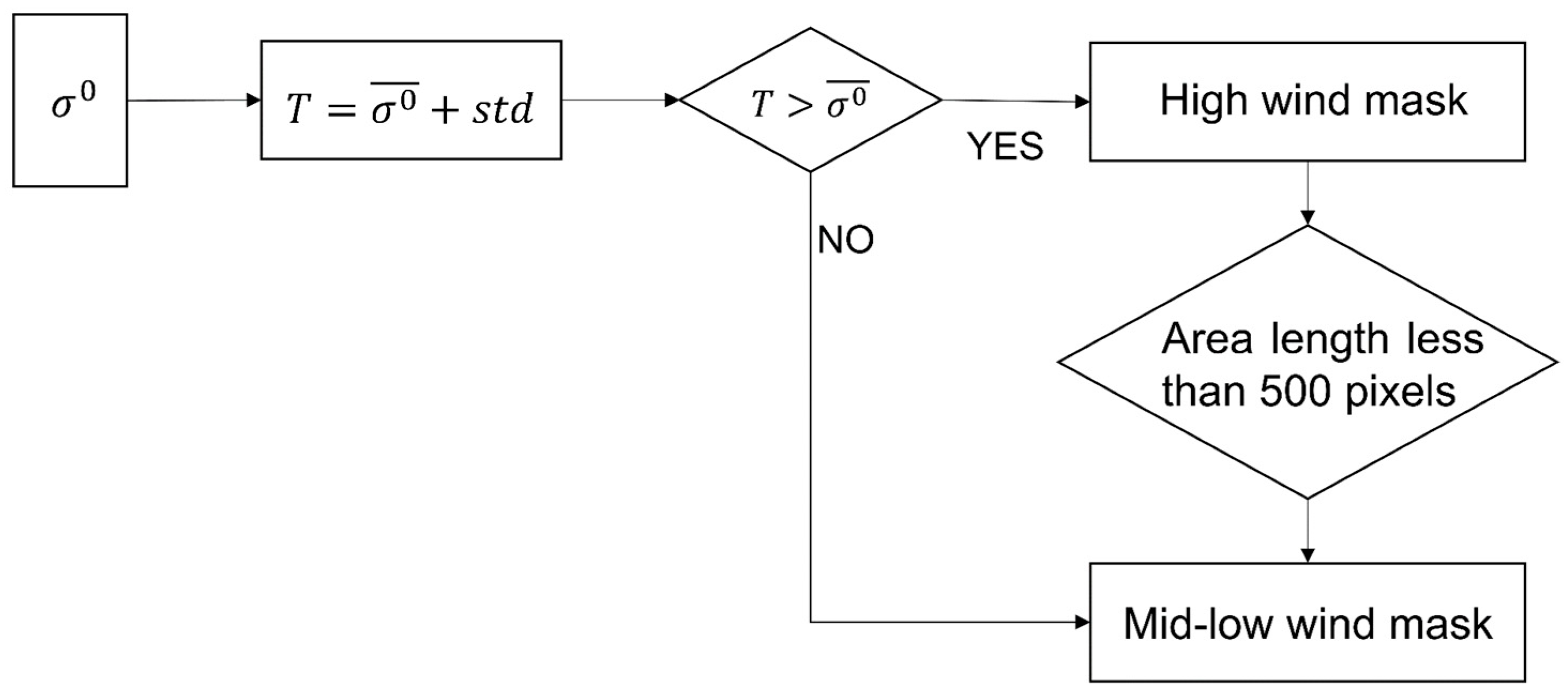
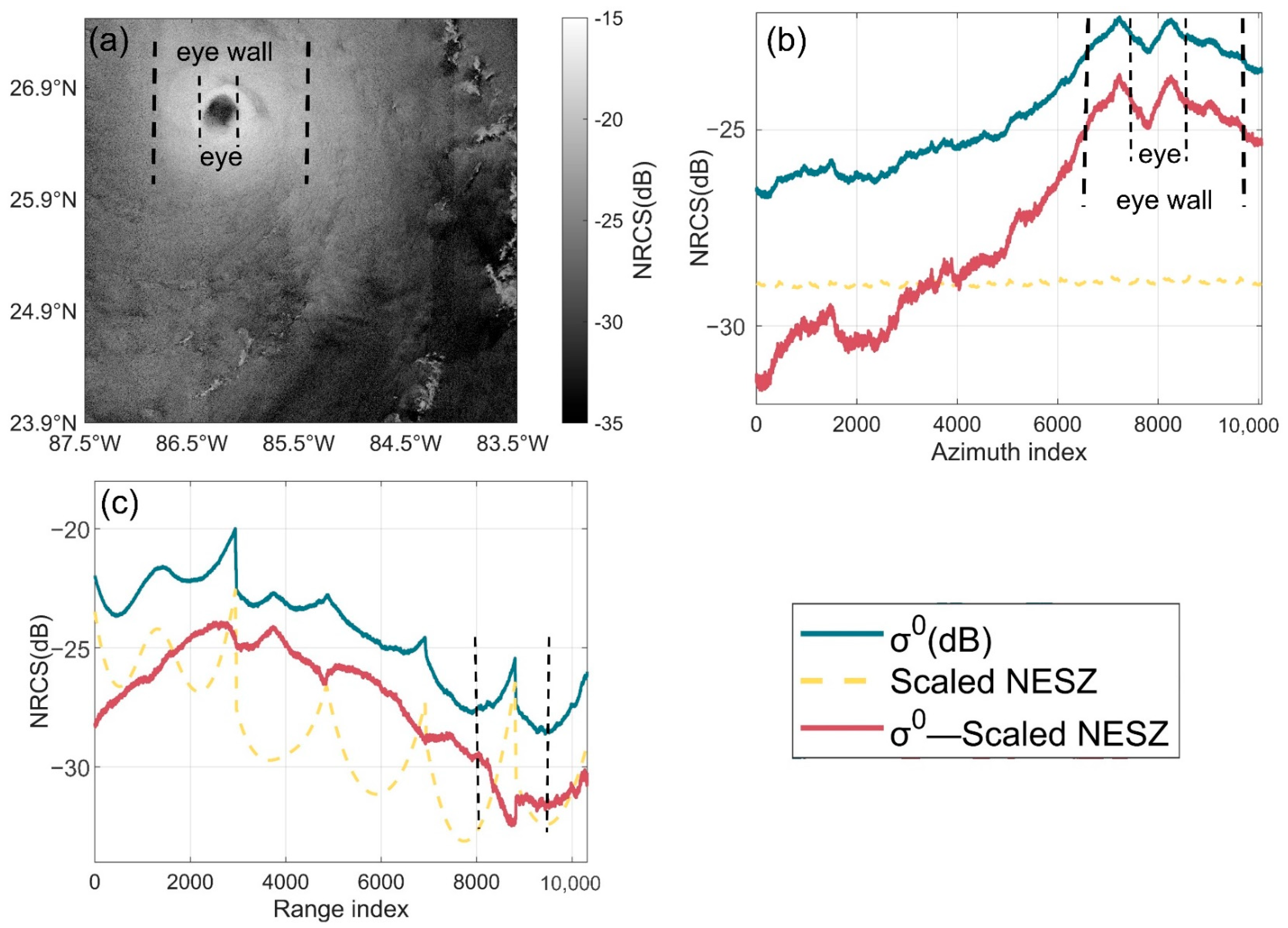
3.1.1. Mid–Low- and High-Wind-Speed Area Blocks

The swath width of the Sentinel-1 EW mode data reaches 419 km and the width of TC eyes typically ranges between 32 and 64 km, while the radius of the outer circulation of a cyclone is generally between 200 and 300 km. Wind speeds vary across different structural regions, increasing towards the eyewall, with relatively lower speeds in the eye and outflow layer. Therefore, in a TC SAR image, areas of high wind speeds and mid–low wind speeds are invariably present. The differences in sea surface roughness caused by these varying wind speed regions lead to significant variations in backscatter intensity and noise levels. Based on the spatial structure of TCs, we propose dividing the TC into the eye, eyewall, and outflow layer regions. Then, a blocking strategy is applied to each sub-swath of the SAR image, with the eye as the center and a buffering zone extending outward to cover the structural regions of the cyclone. This approach enables the separate processing of high-wind-speed and mid–low-wind-speed areas. Building on this approach, the noise-scaling factor for each block is calculated to capture the detailed distribution of noise. This enables a more precise quantification of noise levels in different wind speed regions and various structural parts of the cyclone. By enhancing the adaptability of noise reconstruction, this method addresses potential issues such as over smoothing or inaccuracies that may arise from global processing. The specific implementation method is based on the backscatter characteristics of different wind speeds TC. A statistical feature method using the mean and standard deviation is proposed to effectively divide the high-wind-speed and middle-to-low-wind-speed regions (Figure 5).
T = σ 0 ¯ + s t d
where T is the statistical threshold, σ 0 ¯ is the mean of the backscatter coefficient, and s t d is the standard deviation. After applying the threshold for classification, regions in the mask with a connected area smaller than 500 are filtered out, resulting in separate masks for high-wind-speed and middle-to-low-wind-speed regions. Next, to improve computational efficiency and capture local details, the wind speed regions are further divided into blocks of 500 × 500 size. The eye region is identified, and a block is set for the eye. From the eye’s block, a buffering zone extends outward, resulting in separate blocks for the eyewall’s high-wind-speed region and the eye outflow layer’s mid–low-wind-speed regions.

3.1.2. Optimal Noise-Scaling Factor K s Calculation

The calculation of the optimal noise-scaling factor K s consists of three main steps. First, in order to better reflect the changing characteristics of local noise, calculate the minimum weighted linear residual sum of squares (RSS) for each block. Next, based on the RSS, a likelihood function and prior distribution for the scaling factor are constructed, and Bayesian inference is applied to deduce the posterior distribution characteristics of the noise-scaling factor. Finally, the value with the highest posterior distribution probability is selected as the noise-scaling factor K s , making the noise-scaling factor estimation more stable.
(1) RSS calculation: Fit σ s c , i 0 based on the range direction index and calculate the minimum value of the linear residual sum of squares. The absolute gradient of the NESZ noise vector is used as the fitting weight to more accurately capture the characteristics of the noise vector.
σ s c , i 0 = σ 0 k · G d s · σ N E S Z 0
R S S k = i ω i · f i t ( σ s c , i 0 ) σ s c , i 0 2
where σ s c , i 0 represents the backscatter factor after noise suppression within the block, using the initial noise-scaling factor, and k is the initial scaling factor set within the block, which is set to a step of 0.01 and a range of 0.8–2 based on existing experience [38]. R S S k represents the minimum weighted linear residual sum of squares; i is each block, representing the i _ t h block; ω i is the weight, determined by the absolute of noise gradient, which reflects the detailed variations in the noise; f i t ( σ s c 0 ) is the fitting result of σ s c 0 within the block in relation to the range direction index.
(2) Construct the likelihood function of the noise-scaling factor L σ 0 | k and the prior distribution function p k : In the absence of a precise noise-scaling factor distribution, a prior assumption is made for the scaling factor, and constraints are applied to the estimation process to optimize the estimation of the noise-scaling factor. Using R S S k , construct L σ 0 | k and p k . The maximum likelihood value is calculated when the weighted linear residual sum of squares is minimized.
L σ 0 | k exp R S S k 2 σ v a r 0 2
p k = 1 2 π τ 2 exp ( k μ k ) 2 2 τ 2
where σ v a r 0 is the variance of the initial noise vector within the block, τ is the prior variance distribution of the initial noise vector within the block, and μ k is the prior mean of the initial scaling factor within the block. Set a larger prior variance τ for the scaling factor to express its uncertainty.
(3) Scaling factor posterior distribution estimation: By combining the likelihood function with the distribution of weak prior information, the scaling factor’s posterior distribution is inferred using Bayesian estimate. This approach captures the uncertainty of the noise-scaling factor and estimates its possible probability distribution.
p k σ 0 L σ 0 | k · p k
l o g p k σ 0 = R S S k 2 τ 2 k μ k 2 2 τ 2
Unlike the unique value obtained by minimizing the weighted linear residual sum of squares, the Bayesian estimation method yields the posterior distribution of the scaling factor. From this posterior distribution, the value with the highest probability is selected as the scaling factor K s , i for the block.
K s , i = a r g max k l o g p k σ 0
After obtaining the scaling factor K s , i for each block, the mean scaling factor for the high-wind-speed and mid–low-wind-speed blocks within the sub-swath is calculated and used as the scaling factor for that sub-swath.
K s = i K s , i ¯
where K s is the optimal scaling factor for a sub-swath, which is the mean of all the scaling factors for the wind speed blocks. Taking TC Michael’s cross-pol SAR image as an example, the scaling factors for the five sub-swaths obtained through Bayesian estimation are 1.2794, 0.9902, 0.9639, 1.1714, and 1.05. The denoising result after applying the noise-scaling factor is shown as σ s c 0 (Figure 6a), where the periodic scalloping noise in the azimuth direction within the sub-swaths has been effectively suppressed (Figure 6b). After the suppression of scallop noise, the image no longer exhibits periodic light–dark variations in the azimuth direction. The signal distribution becomes more continuous and realistic, and after removing the noise contribution, the overall signal intensity returns to the correct level. But in the transition area between sub bands (the region between the dashed lines in Figure 6c), range direction noise between the strips still exists. We further calculated the power balance signal between the strips to alleviate the power discontinuity between the strips, thus achieving noise suppression between the strips.

3.1.3. Optimal Power Balance Factor K b Calculate

The power balance factor can balance the power on both sides of the sub-swath edges, reducing the power discontinuities between adjacent sub-swaths. The power balance factor K b is similarly calculated in three main steps [38]. First, identify the region of power discontinuity between sub-swaths. Next, calculate the average power of all the mid-low-wind-speed blocks within the selected region. Finally, correct the power balance signal.
(1) Identify the sub-swath power discontinuity region: Extract the sub-swath boundaries from the data product files, and then select 20 columns of data to the left and right of each boundary, as expressed in Equations (12) and (13).
s t a r t l e f t = min l a s t R a n g e S a m p l e s u b 1 + 20 : 1
s t a r t r i g h t = max f i r s t R a n g e S a m p l e s u b + 1 : 20
where s t a r t r i g h t and s t a r t l e f t represent the data boundaries at the extracted edges. The variable s u b corresponds to sub-swaths 2, 3, 4, and 5. The parameters f i r s t R a n g e S a m p l e and l a s t R a n g e S a m p l e can be obtained from the XML files in the data product.
(2) Calculate the average power of all mid–low-wind-speed blocks within the selected region.
σ b , j 0 = 1 N j σ s c 0 s t a r t r i g h t , j 1 N j σ s c 0 s t a r t l e f t , j
where σ s c 0 is the result after subtracting the scaled noise vector, j denotes the block within the selected region, σ b , j 0 is the balancing factor for the j _ t h block in the selected region, and N is the total number of pixels in the selected region. Calculate the average of the balanced signals of all the blocks in the sub-swath as the power balance factor for that sub-swath:
σ b 0 = j σ b , j 0 ¯
where σ b 0 represents the mean of all balancing factors, serving as the power-balancing factor for the sub-swath.
(3) Correction of power-balancing factor: The noise-scaling factor and power balance factor may lead to changes in the backscattering characteristics of the SAR image signal; in order to avoid changes in the signal power caused by the noise vector modification process and to maintain the overall consistency of the backscattering coefficients, the power in the noise is corrected. The average power difference between the original backscatter coefficient and the scaled noise is integrated into the calculation of the power-balancing factor, resulting in the final power-balancing factor K b .
K b = σ b 0 + σ 0 K s · G d s · σ N E S Z 0 + σ b 0 ¯
After calculating the noise-scaling factor and power-balancing factor, a noise field can be reconstructed using Equation (1), as shown in Figure 7. Figure 7a illustrates the noise field calculated using the ESA noise vector, while Figure 7b shows the two-dimensional noise field reconstructed using the Bayesian method to calculate the noise-scaling and power-balancing coefficients proposed in this study. The reconstructed noise field captures more detailed noise information, closely resembling the actual noise distribution in the image shown in Figure 1.

3.2. Cross-Pol Wind Speed Retrieval Model

The S1EW.NR cross-pol model based on ERA5 reanalysis data and H*Wind data takes into account noise suppression and uses different retrieval methods depending on the incidence angle, enabling a more accurate retrieval of SSWS [36]. So, this cross-pol model is used in this study for SSWS retrieval under TC condition, it writes as follows:
σ 0 d B = 0.52 U 10 32.34 ,     19.75 ° θ < 27.55 °       92.78 U 10 0.45 ,             27.55 ° θ < 37.95 °       80.97 U 10 0.39 ,             37.95 ° θ < 46.95 °
where σ 0 d B represents the backscattering in decibels, and θ is the incident angle. S1EW.NR divides the incident angle range into three parts for wind speed retrieval. Depending on the incident angle function, linear functions and power law functions are used to retrieve the SSWS. The effective retrieval wind speed exceeds 30 m/s, with a bias of −0.11 m/s.

4. Results of Denoise and Wind Speed Retrieval

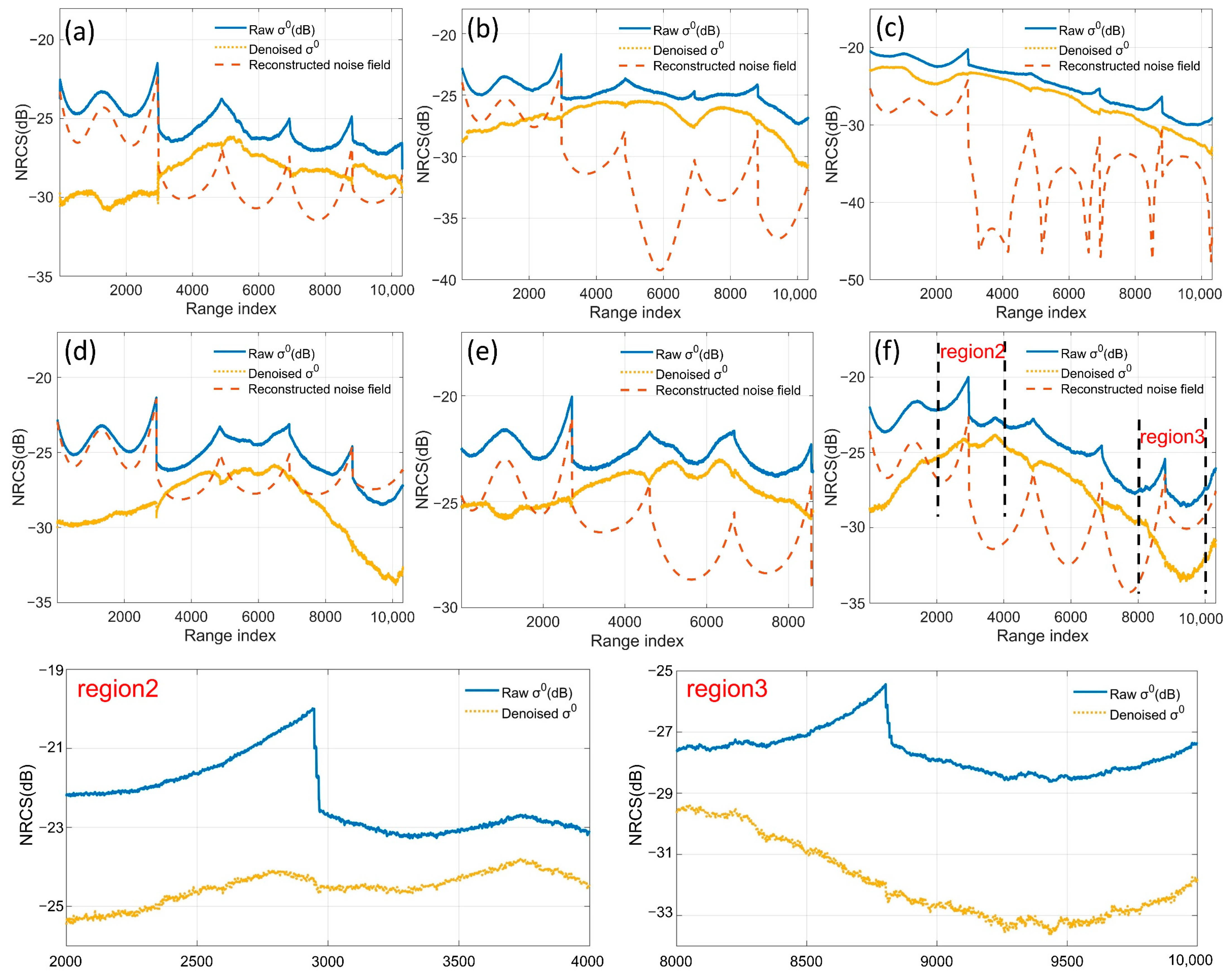
4.1. Noise Suppression Effect of Reconstructed 2D Noise Field

The inherent noise in the original NRCS images not only degrades the visual quality but also obscures the structural features of TCs, resulting in blurred boundaries and hindering the accurate identification of the cyclone eye. This compromises the precise representation of the wind field’s spatial structure and dynamics (Figure 8, first and third columns). After denoising, significant azimuthal noise and inter-swath discontinuities are effectively suppressed (Figure 8, second and fourth columns). Consequently, the structural boundaries of the TC, particularly the eye region, become clearer and more distinguishable. In the six TC cases analyzed, noise amplification causes the signal power of the first sub-swath to reach as high as –20 dB, with elevated power levels observed between sub-swaths—sometimes approaching the echo power of the high-wind eyewall region. Notably, TC Douglas exhibits the highest average noise level (Figure 8(d1)), with the signal power of the first sub-swath reaching –15 dB, corresponding to the backscatter of a wind speed of 33.4 m/s. After denoising, the power of the first sub-swath is significantly reduced, and the corresponding wind speed drops to approximately 14.1 m/s—consistent with the characteristics of the outflow layer. Moreover, the boundaries between the eye and the eyewall become more distinct, revealing finer structural details. Across TCs of varying intensities, the denoised cross-pol NRCS substantially enhances data visualization (Figure 8).
Figure 9 illustrates the effects of noise suppression in the azimuth direction for six TC images. Overall, the raw signals exhibit substantial periodic fluctuations across all cases. After applying the denoising process, these fluctuations are significantly reduced, while the underlying signal trends are well preserved. In the C3 and C4 cases, which show relatively high average noise levels in the raw data (Figure 9d,e), the reconstructed azimuth noise also reflects higher intensities, reaching approximately –26 dB. In contrast, the C2 dataset has a noticeably lower noise level (Figure 9c). After reconstruction, the denoised results align more closely with the true backscattering trend, indicating that the noise field reconstruction is effectively modulated by the inherent mean noise level of the original SAR imagery. In “region 1”, the raw backscatter curve exhibits prominent periodic fluctuations. After denoising, these fluctuations are effectively removed, and the denoised signal accurately follows the trend of the original backscatter, providing a closer approximation to the true signal.
We further conducted a quantitative evaluation of noise suppression in the range direction for six TCs, as illustrated in Figure 10. The raw NRCS profiles display notable intensity fluctuations, particularly in the transition zones between adjacent sub-swaths, where localized peaks are observed. These peaks indicate the presence of strong noise components and pronounced noise amplification. In contrast, the reconstructed noise field effectively captures these noise characteristics. The peak positions in the reconstructed noise profiles closely align with those in the raw NRCS, demonstrating the accuracy of the noise field reconstruction. Additionally, the denoised NRCS shows significantly reduced power levels and a smoother overall profile. The noise components are largely eliminated, with the denoised NRCS values generally concentrated in the range of –25 dB to –30 dB. As shown in Figure 10a, the transition zones between the five sub-swaths are located near column indices 3000, 5000, 7000, and 9000, where clear backscatter discontinuities occur. For instance, at column index 3000—the boundary between the first and second sub-swaths—the raw NRCS exhibits a sharp contrast of approximately 5 dB. After denoising, the NRCS curve becomes more stable, effectively mitigating the power discontinuity across the swath boundary. In “region 2”, the raw NRCS declines from approximately –20 dB to –23 dB, whereas the denoised NRCS remains stable around –25 dB, presenting a more consistent trend. Similarly, in “region 3”, the raw NRCS shows a sudden increase of about 2 dB, while the denoised NRCS remains steady between –29 dB and –30 dB, yielding a smooth transition and minimizing discontinuities.

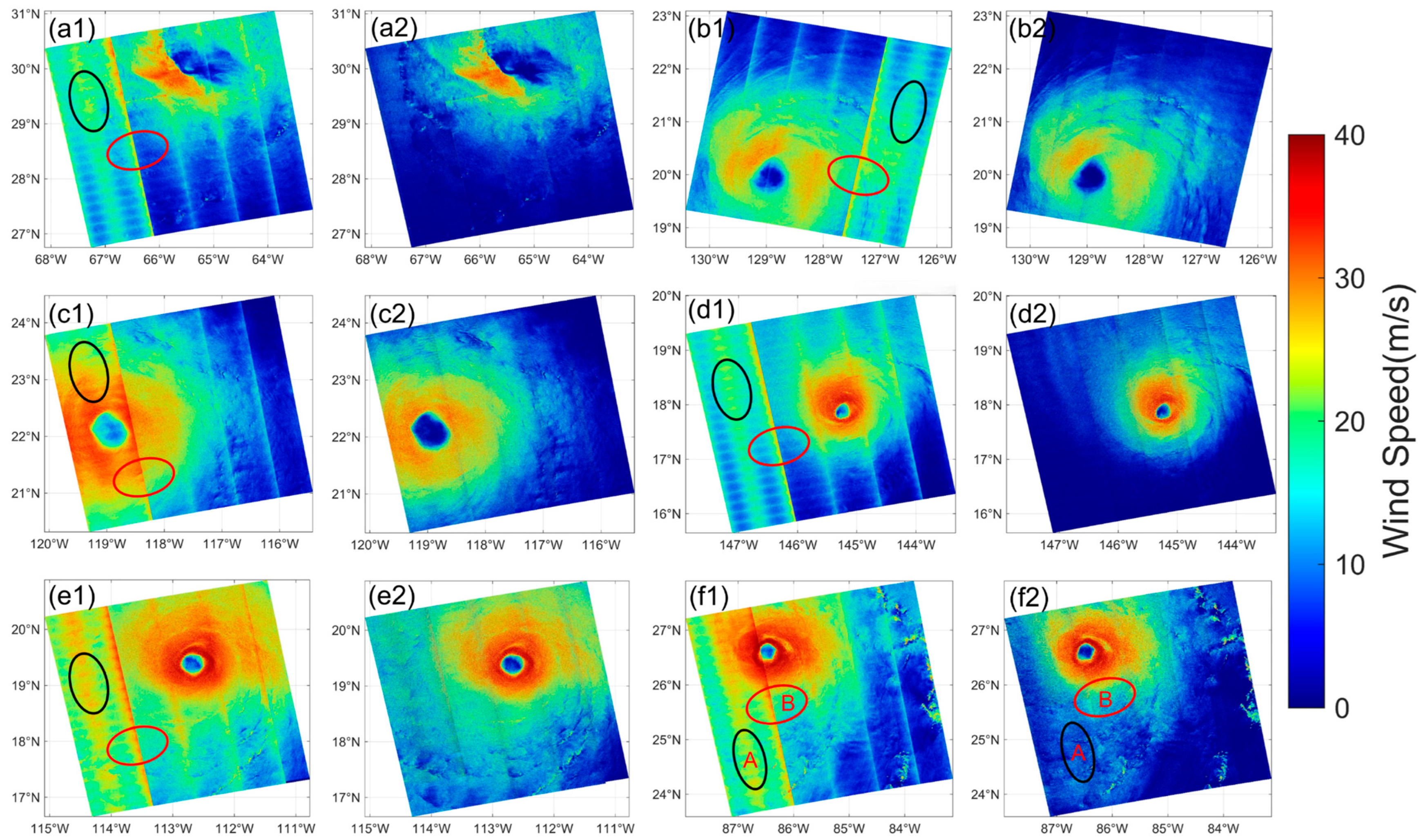
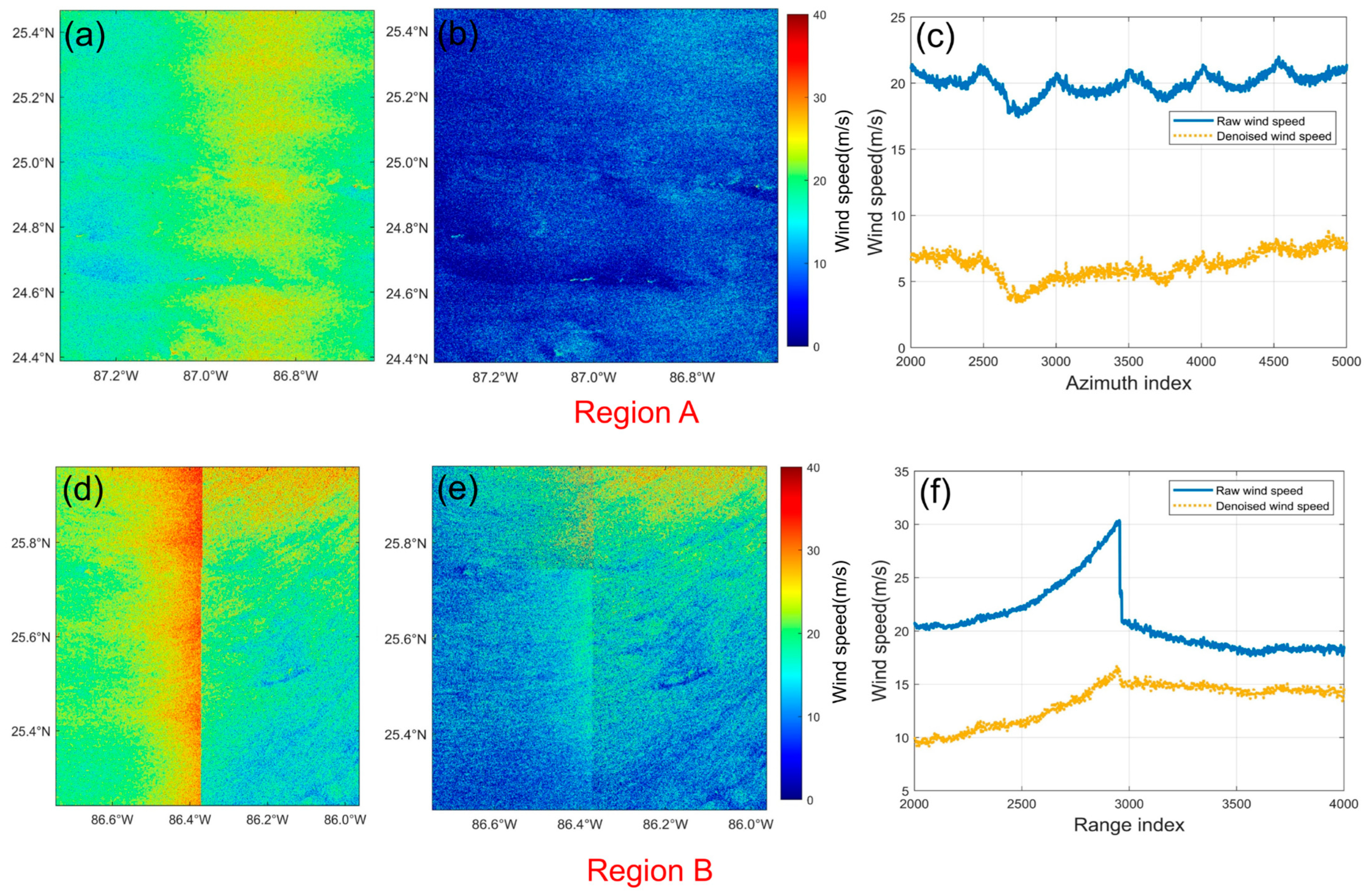
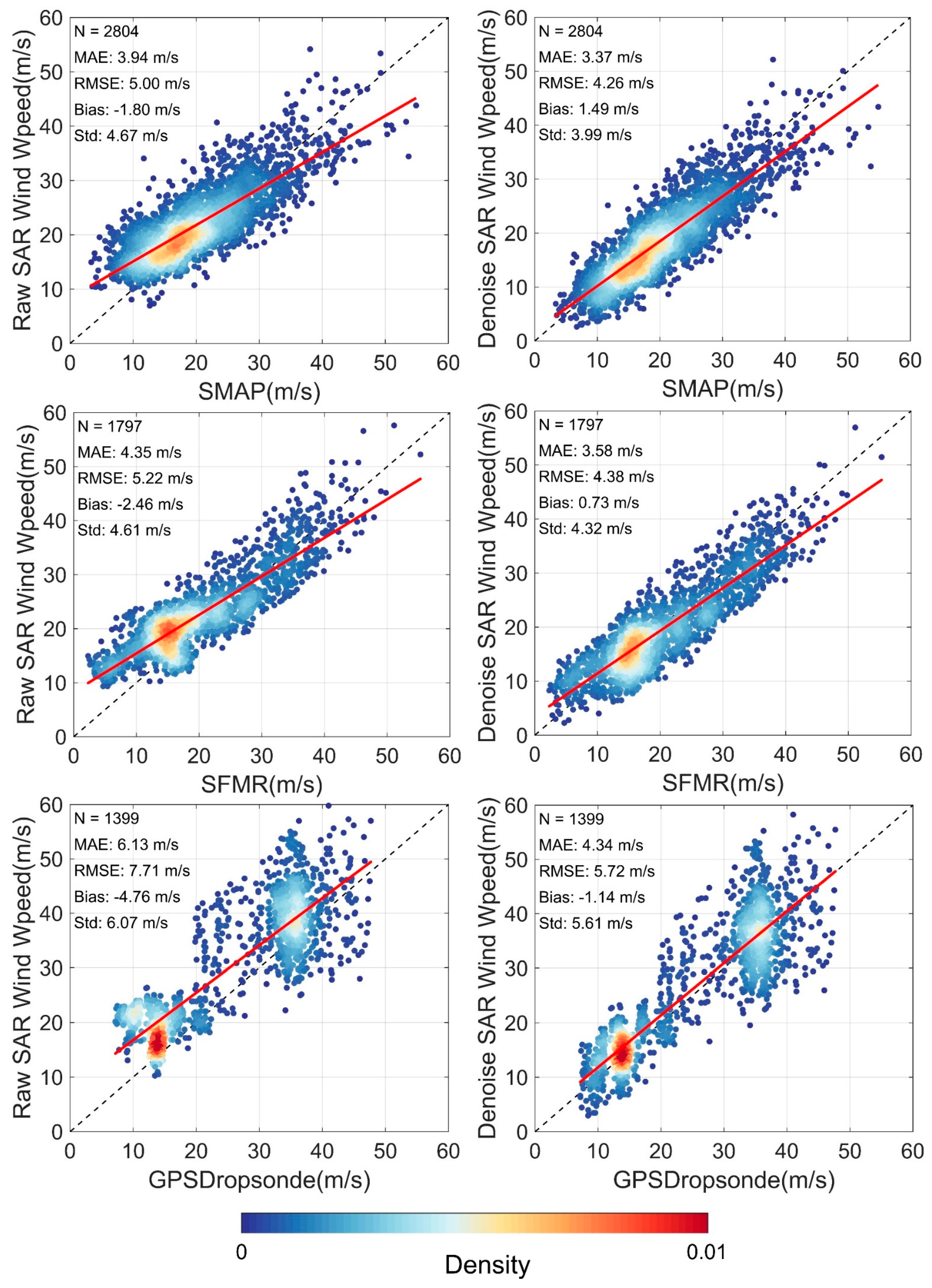
4.2. Results of Wind Speed Retrieval

The wind speed retrieval results for six TCs, ranging from tropical storm (TS) to Category 5 (C5), are presented in Figure 11. Overall, directly retrieving wind speed from raw SAR images introduces substantial noise into the results. As highlighted by the black ovals in Figure 11, this noise induces periodic fluctuations along the azimuth direction, resulting in unrealistic wind speed variations and marked spatial inhomogeneity. Moreover, abnormally high wind speeds—comparable to those within the eyewall—are retrieved in the outflow layer, where lower wind speeds are expected, indicating physically implausible results. Along the range direction (as marked by red ellipses in Figure 11), the wind speed field exhibits discontinuous jumps between sub-swaths, undermining spatial coherence. The presence of noise also leads to a blurred eyewall boundary and an unclear structural definition, distorting the wind speed gradient and its correspondence to the actual wind field. After applying denoising, as shown in the second and fourth columns of Figure 11, both visual and quantitative improvements are evident. In the azimuth direction, noise suppression eliminates the periodic fluctuations, resulting in a smoother and more realistic wind speed distribution that better reflects the continuous transition from the outflow layer to the eyewall. In the range direction, abrupt inter-swath discontinuities are effectively reduced, leading to a more coherent and consistent spatial wind speed field.
After denoising, local improvements in wind speed retrieval are also evident. Within individual azimuth sub-swaths, the presence of periodic azimuth scalloping noise causes the retrieved wind speeds to exhibit periodic fluctuations (Figure 12a,c). In the outflow layer of region A, however, the actual wind field should be relatively uniform without such localized variations. This inconsistency arises from the periodic nature of the noise in region A, which contributes additional power to the measured NRCS. Consequently, the NRCS input to the retrieval model is overestimated, resulting in retrieved wind speeds that exceed the actual values by more than 10 m/s. After denoising (Figure 12b), the retrieved wind speed in region A—represented by the yellow curve in Figure 12c—shows significantly reduced fluctuations and better reflects a uniform wind field. The removal of noise-induced power effectively lowers the retrieved wind speed values and improves the physical consistency of the retrieval results.
At the edges of sub-swaths, noise leads to abrupt changes in NRCS, resulting in noticeable discontinuities in the retrieved wind speed, as illustrated in Figure 12d. In region B, the pre-denoising wind speed distribution—depicted by the blue curve in Figure 12f— exhibits a sharp 10 m/s jump at the sub-swath boundaries. However, based on the empirical characteristics of tropical cyclone wind fields, such a large wind speed difference across adjacent pixels is unrealistic; the wind speed should remain relatively continuous, or with only minor variations. After denoising (Figure 12e), the retrieved wind speed distribution in region B, shown by the yellow curve in Figure 12f, becomes significantly smoother. The sharp jump at the sub-swath boundary is greatly reduced, and the retrieved values align more closely with the expected physical behavior of the wind field.

5. Discussion

5.1. Noise Suppression Effect of 2D Noise Field Reconstruction

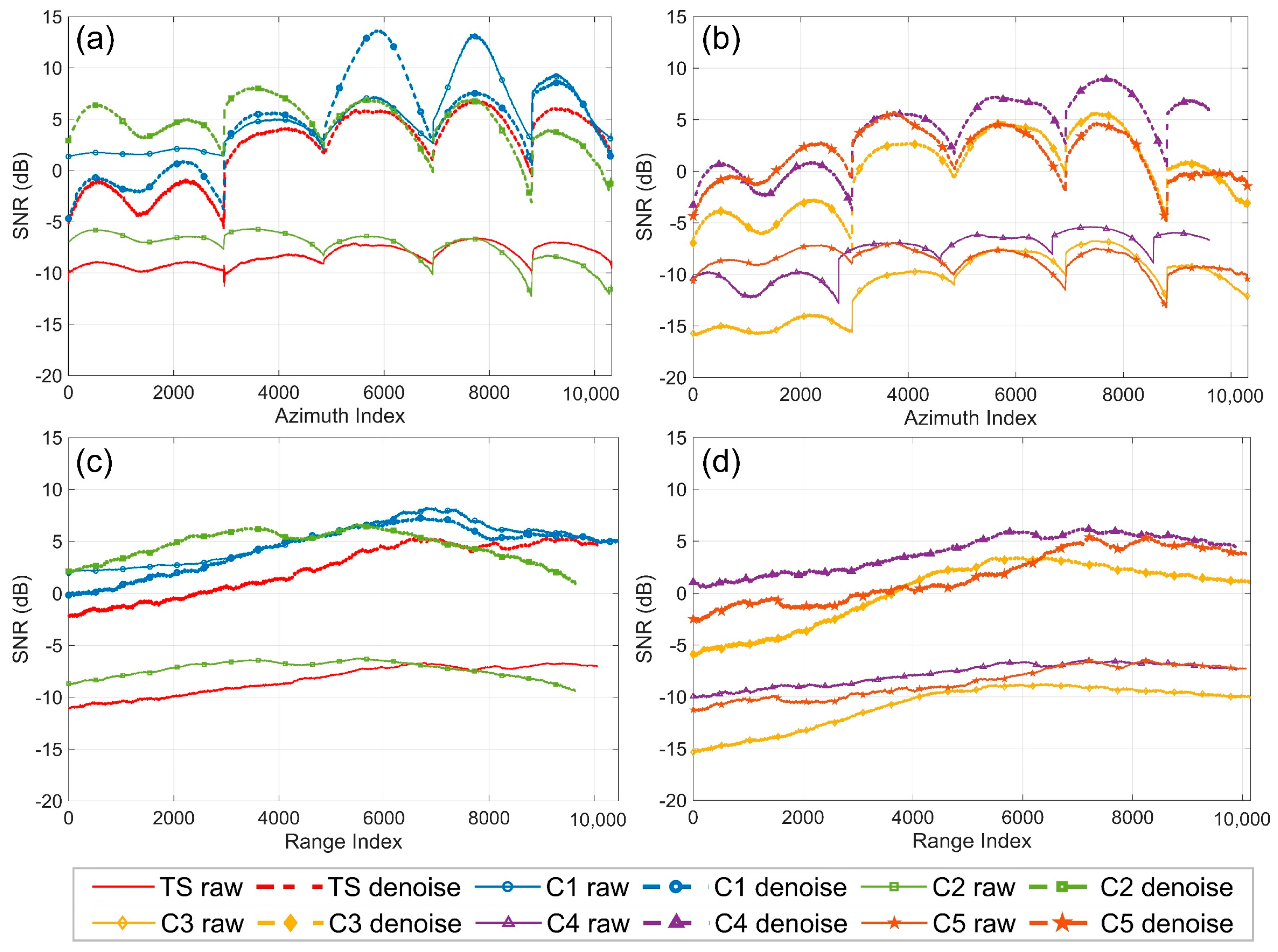
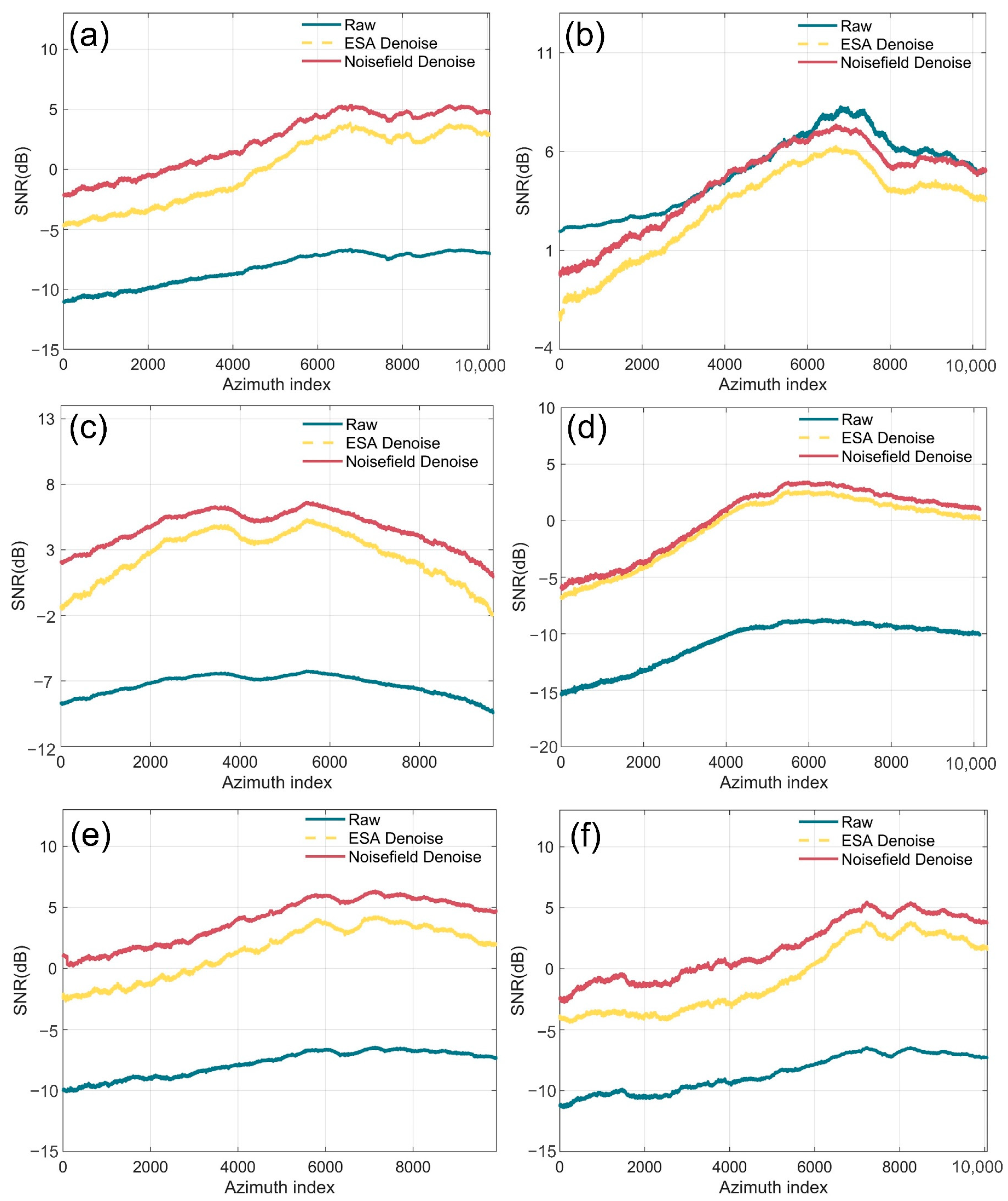
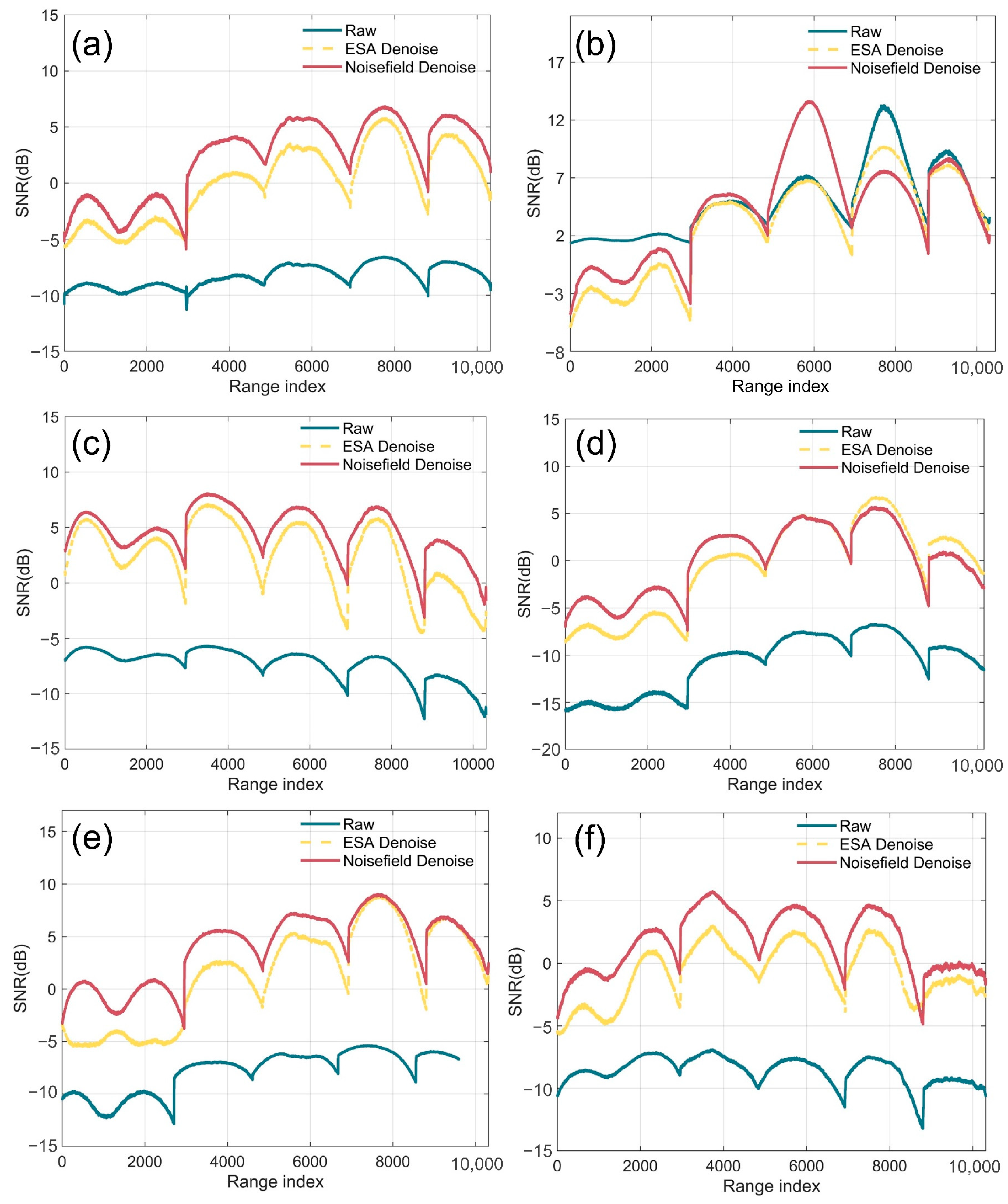
5.1.1. SNR Analysis of SAR Before and After Noise Removal

The specific calculation formula for the signal-to-noise ratio (SNR) in Sentinel-1 data is as follows:
S N R = 10 × log 10 ( ( σ 0 σ N E S Z 0 ) / σ N E S Z 0 )
Figure 13 presents the changes in SNR before and after denoising for different TCs in both the azimuth and range directions. Overall, the proposed denoising method leads to improved SNR across all cases, though the degree of enhancement varies among different TCs. In the azimuth direction, the SNR improvement is generally consistent, with particularly notable gains observed for TCs C4 and C5, where the SNR increases by more than 6 dB. In contrast, for C1 and C2, the lower raw noise levels limit the improvement in SNR, resulting in more modest gains. In the range direction, the denoising performance shows greater variability. For TCs C1 (Marie) and C2 (Rosa), the raw noise level is approximately –30.5 dB, and the SNR improvement is modest, increasing by just over 2 dB. Conversely, for TC C3 (Douglas), which has the highest raw noise level at –26.4 dB and a low original SNR of –10.81 dB, the denoising yields a substantial improvement. The average SNR rises to 0.16 dB after denoising, corresponding to a gain of 10.97 dB.

5.1.2. Comparative Analysis with ESA Noise Vectors

The ESA noise vector is one of the most widely used denoising methods for SAR data and can effectively suppress noise to a certain extent. For six TCs, ranging from TS to C5 intensity, a quantitative comparison was conducted among the original SNR, the SNR after ESA denoising, and the SNR after applying the proposed two-dimensional noise field denoising method (Figure 14 and Figure 15). Overall, the proposed method yields an average SNR improvement of 2.54 dB compared to the ESA denoising approach.
In azimuth direction, the raw SNR values range from −15 dB to −7 dB. After applying the ESA denoising method, the SNR improves to between −5 dB and 6 dB. Using the proposed two-dimensional noise field denoising method, the SNR is further enhanced to a range of −5 dB to 7 dB, which is overall higher than that achieved with ESA denoising (Figure 14). However, for the C3 TC Douglas (Figure 14d), the SNR after applying the proposed method is nearly identical to that obtained with ESA denoising. This may be attributed to the high average noise level of this dataset (approximately −26.4 dB), which allows the ESA noise vector to capture a substantial portion of the noise, resulting in a performance comparable to the proposed method.
In range direction, the SNR in the first sub-swath typically reaches its lowest value around column 3000, which marks the transition between the first and second sub-swaths. Both ESA denoising and noise field denoising results exhibit a high degree of consistency with the variation trend of the raw SNR. The raw SNR in the range direction ranges from −15 dB to −5 dB. After applying ESA denoising, the SNR improves to a range of −10 dB to 5 dB, whereas the noise field-based denoising method achieves a SNR distribution is −5 dB to 10 dB, demonstrating the significant enhancement. In the transition region of the range sub-swath, the SNR after noise field denoising is consistently higher than that after ESA denoising, effectively suppressing the noise between sub-swaths. As shown in Figure 15d,e, the SNR values after ESA denoising and noise field denoising are nearly identical in the first sub-swath transition region. Similarly, in the fourth and fifth sub-swaths of Figure 15d, the SNR after ESA denoising is slightly higher than that after noise field denoising. This discrepancy may be attributed to over-denoising in these regions.
It is worth noting that in some regions, the raw SNR is better than the denoised SNR. In C1 TC (Figure 15b), there are areas where the raw SNR is significantly higher than the denoised SNR, and a similar phenomenon is also observed in the azimuth direction.

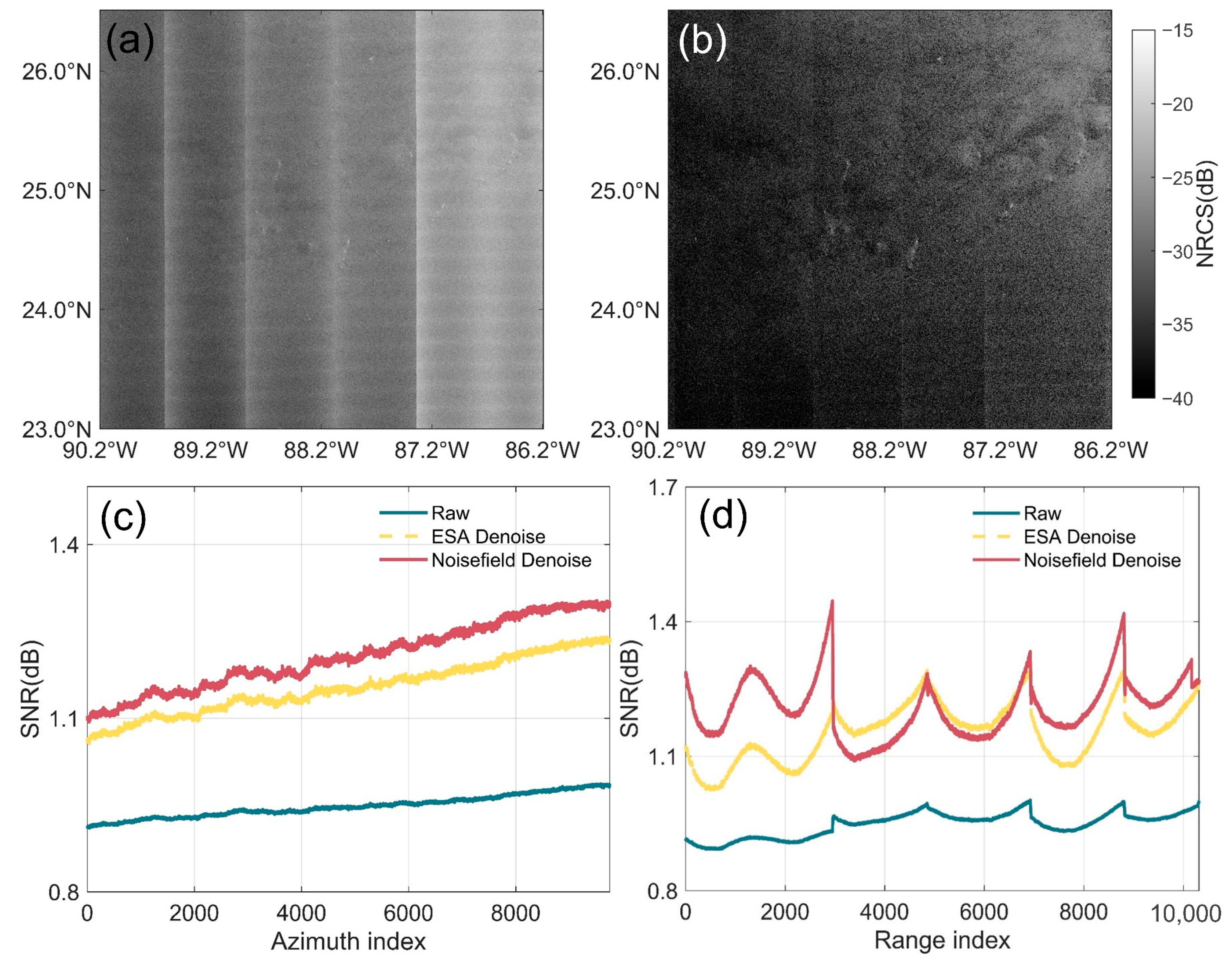
5.1.3. Denoising Results of Non-TC SAR Data

The Sentinel-1 cross-pol SAR data under non-TC condition in same region were selected, and the cross-pol backscattered signals under calm seas were weaker, with more pronounced noise textures in the azimuth and range directions, and a greater degree of noise influence, resulting in poorer-quality data (Figure 16a). Using the methodological process in this paper for denoising (Figure 16b), the textural characteristics of the noise are no longer apparent, the noise texture of the light and dark variations within the data has been effectively suppressed, and the continuity of the data has been significantly improved. By comparing the raw data, ESA denoised data, and noise field denoised data, it is found that the denoising effect of the method presented in this paper is superior to that of the ESA noise vector. The SNR improvement is higher with this method than with the ESA noise vector, and it also demonstrates good denoising performance and stability under non-TC conditions.

5.2. Discussion of TC Wind Speed Retrieval Results

5.2.1. Effect of SAR Noise on TC Wind Speed Retrieval

Since the wind measurements from SFMR, GPS Dropsondes, and NDBC buoys are not taken at 10 m height, this study employs the exponential wind shear model to convert wind speeds from various heights to 10 m equivalents for consistency.
V 10 = V 0 H 10 H 0 α
In above equation, V 10 represents the wind speed at a height of 10 m, V 0 is the observed wind speed at height H 0 , and α is the wind shear exponent, which is set to 0.143 in this study.
Wind speed retrieval was conducted using denoised cross-pol Sentinel-1 images from 15 TC cases and validated against SMAP, height-converted SFMR, GPSDropsonde, and NDBC buoy measurements (Figure 17). The results clearly demonstrate improved retrieval accuracy after applying the denoising method. Compared to SMAP data, the RMSE, bias, and MAE were reduced by 0.74 m/s, 0.31 m/s, and 0.57 m/s, respectively. For SFMR comparisons, the corresponding improvements were 0.84 m/s, 1.73 m/s, and 0.77 m/s. When validated against GPSDropsonde and NDBC buoy observations, the denoising yielded more pronounced enhancements, with RMSE, bias, and MAE reductions of 1.99 m/s, 3.62 m/s, and 1.79 m/s, respectively. These findings indicate that the proposed denoising approach exhibits strong robustness in mitigating errors and biases in high-wind-speed retrieval under TC conditions.
The effectiveness of the denoising method varies across different wind speed intervals (Table 2). In below 30 m/s range, noise-induced errors are more prominent, as indicated by the higher dispersion of scatter points and their deviation from the validation trend, often exceeding the reference values. After denoising, noise amplification is significantly suppressed, leading to a marked improvement in retrieval accuracy. The RMSE is reduced by 20.2%, the bias decreases to 1.11 m/s, and the scatter points become more concentrated around the validation curve, demonstrating improved consistency. In the high wind speed regime (≥30 m/s), the wind speed retrieval results also exhibit clear improvements. After denoising, the bias is reduced to 0.79 m/s. Across all wind speed intervals, the denoised retrievals outperform the original results: the overall bias decreases to 0.65 m/s, and the R2 increases to 0.88. These results indicate that the proposed denoising method enhances wind speed retrieval accuracy across both moderate and high wind conditions, effectively minimizing retrieval errors.

5.2.2. Other Factors Affecting the Accuracy of TC Wind Speed Retrieval

Many existing cross-pol GMFs estimate SSWS based on empirical relationships among backscatter, wind speed, and incidence angle. While these models have demonstrated operational utility, their outputs are highly sensitive to parameter variations, and any changes in model inputs can propagate significant uncertainties into wind speed retrieval. In cross-pol channels, the normalized radar cross section (NRCS) is primarily correlated with wind speed when the effect of incidence angle is neglected. However, empirical observations over an incidence angle range of 19.5° to 49.5° indicate a clear linear decrease in NRCS with increasing incidence angle [39]. This trend suggests that variations in incidence angle intrinsically alter the backscatter response. Therefore, excluding the incidence angle dependence from GMFs introduces systematic biases, ultimately degrading the accuracy of wind speed retrieval.
Under TC conditions, the sea surface becomes highly turbulent, and widespread wave breaking makes foam scattering the dominant mechanism for cross-pol backscatter. Foam contributions can account for as much as 60–80% of the cross-pol NRCS [40,41]. Therefore, properly accounting for the influence of breaking waves is essential for improving the accuracy of NRCS modeling and SSWS retrieval in cross-pol channels [42]. In addition, TCs are typically accompanied by intense precipitation, which not only enhances sea surface roughness but also affects cross-pol NRCS through atmospheric signal scattering and attenuation by raindrops. At a rainfall rate of 20 mm/h, cross-pol NRCS can attenuate by approximately 2.2 dB [43], significantly impacting wind speed retrieval accuracy. Within rain cells, the influence of precipitation on co- polarization channels is generally weaker than on cross-pol channels [44], further exacerbating retrieval errors. However, current cross-pol-based retrieval models rarely incorporate external environmental factors such as wave breaking and precipitation, thereby limiting their accuracy under extreme weather conditions.

6. Conclusions

To address the significant impact of noise in cross-pol SAR data on the accuracy of wind speed retrieval, this study proposes a noise suppression method based on TC structural characteristics. The proposed method includes three main components: cyclone structure-based segmentation, noise-scaling coefficient estimation, and power balance coefficient calculation. This approach effectively suppresses noise in cross-pol SAR data under the complex oceanic conditions associated with TCs. The results demonstrate notable improvements in both visual quality and SNR, with the overall SNR increasing by an average of 9.15 dB compared to the original data, and 2.54 dB higher than the denoising method provided by the ESA noise vector. Building on this, the S1EW.NR model is applied for TC wind speed retrieval, showing that the proposed denoising approach significantly enhances retrieval accuracy. Specifically, the wind speed bias is reduced from −2.69 m/s to 0.65 m/s, and the R2 improves to 0.88. To further enhance the accuracy of sea surface wind speed retrieval under TC conditions, future work may incorporate multi-source satellite data assimilation to integrate diverse observations and optimize retrieval performance.

Author Contributions

D.G.: Writing—review and editing, supervision, project administration, conceptualization. L.W.: Writing—original draft. W.S.: Writing—review and editing, project administration. H.W.: Writing—review and editing. W.J.: Writing—review and editing. T.F.: Writing—review and editing. All authors have read and agreed to the published version of the manuscript.

Funding

This work was funded by the National Natural Science Foundation of China (No. 42176174), Ningbo Yongjiang Talent Introduction Programme (No. 2021A-136-G), Key Technology Breakthrough Plan of Ningbo Science and Technology Innovation 2035 (No. 2024Z262) and Public Projects of Ningbo City under Grant 2023S102.

Data Availability Statement

Sentinel-1 data from this research will be available on Copernicus Data Space Ecosystem (https://dataspace.copernicus.eu, accessed on 8 April 2024). SMAP data from this research will be available on Remote Sensing Systems (https://www.remss.com/missions, accessed on 29 March 2024). SFMR data and GPSDropsonde data from this research will be available on Atlantic Oceanographic & Meteorological Laboratory (https://www.aoml.noaa.gov/data-products, accessed on 19 June 2024). NDBC data from this research will be available on National Data Buoy Center (https://www.ndbc.noaa.gov, accessed on 3 July 2024).

Acknowledgments

The authors would like to thank the Copernicus Data Space Ecosystem for providing Sentinel-1 data, the Remote Sensing Systems for providing SMAP data, the Atlantic Oceanographic & Meteorological Laboratory for providing SFMR data and GPSDropsonde data, and the National Data Buoy Center for providing buoy data.

Conflicts of Interest

The authors declare no conflicts of interest.

References

  1. Pichel, W.G.; Monaldo, F.M.; Jackson, C.; Li, X.; Sapper, J. NOAA operational SAR winds—Current status and plans for Sentinel-1A. In Proceedings of the 2015 IEEE International Geoscience and Remote Sensing Symposium (IGARSS), Milan, Italy, 26–31 July 2015; pp. 4916–4919. [Google Scholar]
  2. Fernandez, D.E.; Carswell, J.R.; Frasier, S.; Chang, P.S.; Black, P.G.; Marks, F.D. Dual-polarized C-and Ku-band ocean backscatter response to hurricane-force winds. J. Geophys. Res. Ocean 2006, 111. [Google Scholar] [CrossRef]
  3. Mouche, A.; Chapron, B. Global C-Band Envisat, RADARSAT-2 and Sentinel-1 SAR measurements in copolarization and cross-polarization. J. Geophys. Res.-Ocean. 2015, 120, 7195–7207. [Google Scholar] [CrossRef]
  4. Zhang, B.; Perrie, W. Cross-polarized synthetic aperture radar: A new potential measurement technique for hurricanes. Bull. Am. Meteorol. Soc. 2012, 93, 531–541. [Google Scholar] [CrossRef]
  5. Hwang, P.A.; Zhang, B.; Toporkov, J.V.; Perrie, W. Comparison of composite Bragg theory and quad-polarization radar backscatter from RADARSAT-2: With applications to wave breaking and high wind retrieval. J. Geophys. Res. Ocean 2010, 115. [Google Scholar] [CrossRef]
  6. Zhang, B.; Mouche, A.A.; Perrie, W. First quasi-synchronous hurricane quad-polarization observations by C-band radar constellation mission and RADARSAT-2. IEEE Trans. Geosci. Remote Sens. 2022, 60, 1–10. [Google Scholar] [CrossRef]
  7. Yang, J.; Zhong, L.; Yuan, X.; Wang, X.; Han, B.; Hu, Y. First assessment of Noise-Equivalent Sigma-Zero in GF3-02 TOPSAR mode with sea surface wind speed retrieval. Acta Oceanol. Sin. 2023, 42, 84–96. [Google Scholar] [CrossRef]
  8. De Zan, F.; Guarnieri, A.M. TOPSAR: Terrain observation by progressive scans. IEEE Trans. Geosci. Remote Sens. 2006, 44, 2352–2360. [Google Scholar] [CrossRef]
  9. Frank, D.C. (Ed.) Microwave Remote Sensing of Sea Ice; American Geophysical Union: Washington, DC, USA, 1992. [Google Scholar]
  10. Balss, U.; Breit, H.; Niedermeier, A. Computation of signal gain and noise gain of a SAR processor. In Proceedings of the CEOS Strategic Implementation Team (SIT) Technical Workshop, Darmstadt, Germany, 17–18 September 2015. [Google Scholar]
  11. Piantanida, R.; Hajduch, G.; Poullaouec, J. Sentinel-1 Level 1 Detailed Algorithm Definition; Techreport SEN-TN-52-7445; ESA: Paris, France, 2016. [Google Scholar]
  12. Iqbal, M.; Chen, J.; Yang, W.; Wang, P.; Sun, B. Kalman filter for removal of scalloping and inter-scan banding in scansar images. Prog. Electromagn. Res. 2012, 132, 443–461. [Google Scholar] [CrossRef]
  13. Tan, W.; Li, J.; Xu, L.; Chapman, M.A. Semiautomated segmentation of Sentinel-1 SAR imagery for mapping sea ice in Labrador coast. IEEE J. Sel. Top. Appl. Earth Obs. Remote Sens. 2018, 11, 1419–1432. [Google Scholar] [CrossRef]
  14. Kasapoğlu, N.G. Sea ice concentration retrieval using composite ScanSAR features in a SAR data assimilation process. IEEE Geosci. Remote Sens. Lett. 2014, 11, 2085–2089. [Google Scholar] [CrossRef]
  15. Ren, L.; Yang, J.; Mouche, A.; Wang, H.; Wang, J.; Zheng, G.; Zhang, H. Preliminary analysis of Chinese GF-3 SAR quad-polarization measurements to extract winds in each polarization. Remote Sens. 2017, 9, 1215. [Google Scholar] [CrossRef]
  16. Zhang, K.; Zhang, B.; Perrie, W.; Zheng, G.; Yang, J.; Fang, H. Assessment of Thermal Noise Effect on Wind Speed Retrieval Accuracy Using Sentinel-1 Cross-polarized TOPSAR Images. IEEE Trans. Geosci. Remote Sens. 2023, 61, 1–11. [Google Scholar] [CrossRef]
  17. Yang, W.; Li, Y.; Liu, W.; Chen, J.; Li, C.; Men, Z. Scalloping suppression for ScanSAR images based on modified Kalman filter with preprocessing. IEEE Trans. Geosci. Remote Sens. 2020, 59, 7535–7546. [Google Scholar] [CrossRef]
  18. Miranda, N.; Piantanida, R.; Recchia, A.; Franceschi, N.; Small, D.; Schubert, A.; Meadows, P.J. S-1 instrument and product performance status: 2018 update. In Proceedings of the 2018 IEEE International Geoscience and Remote Sensing Symposium (IGARSS), Valencia, Spain, 22–27 July 2018; pp. 1551–1554. [Google Scholar]
  19. Piantanida, R.; Miranda, N.; Franceschi, N.; Meadows, P.; Hajduch, G. Thermal Denoising of Products Generated by the S-1 IPF; DI-MPC-TN, MPC-0392; Sentinel-1 Mission Perform: Ramonville-Saint-Agne, France, 2017. [Google Scholar]
  20. Karvonen, J. Baltic sea ice concentration estimation using SENTINEL-1 SAR and AMSR2 microwave radiometer data. IEEE Trans. Geosci. Remote Sens. 2017, 55, 2871–2883. [Google Scholar] [CrossRef]
  21. Park, J.W.; Korosov, A.A.; Babiker, M.; Sandven, S.; Won, J.-S. Efficient thermal noise removal for Sentinel-1 TOPSAR cross-polarization channel. IEEE Trans. Geosci. Remote Sens. 2017, 56, 1555–1565. [Google Scholar] [CrossRef]
  22. Korosov, A.; Demchev, D.; Miranda, N.; Franceschi, N.; Park, J.-W. Thermal denoising of cross-polarized Sentinel-1 data in interferometric and extra wide swath modes. IEEE Trans. Geosci. Remote Sens. 2021, 60, 1–11. [Google Scholar] [CrossRef]
  23. Park, J.W.; Won, J.S.; Korosov, A.A.; Babiker, M.; Miranda, N. Textural noise correction for Sentinel-1 TOPSAR cross-polarization channel images. IEEE Trans. Geosci. Remote Sens. 2019, 57, 4040–4049. [Google Scholar] [CrossRef]
  24. Lee, P.Q.; Xu, L.; Clausi, D.A. Estimating Noise Floor in Sentinel-1 Images with Linear Programming and Least Squares. IEEE Trans. Geosci. Remote Sens. 2021, 60, 1–14. [Google Scholar] [CrossRef]
  25. Lee, P.Q.; Xu, L.; Clausi, D.A. Sentinel-1 additive noise removal from cross-polarization extra-wide TOPSAR with dynamic least-squares. Remote Sens. Environ. 2020, 248, 111982. [Google Scholar] [CrossRef]
  26. Hu, Y.; Shao, W.; Shen, W.; Zhou, Y.; Jiang, X. Machine learning applied to a dual-polarized Sentinel-1 image for wind retrieval of tropical cyclones. Remote Sens. 2023, 15, 3948. [Google Scholar] [CrossRef]
  27. Zhou, Y.; Shao, W.; Nunziata, F.; Wang, W.; Li, C. An Algorithm to Retrieve Range Ocean Current Speed under Tropical Cyclone Conditions from Sentinel-1 Synthetic Aperture Radar Measurements Based on XGBoost. Remote Sens. 2024, 16, 3271. [Google Scholar] [CrossRef]
  28. Shao, W.; Wei, M.; Hu, Y.; Marino, A.; Jiang, X. Wind speed retrieval approach for VV-polarized synthetic aperture radar during tropical cyclone based on XGBoost model. Int. J. Remote Sens. 2024, 45, 4367–4384. [Google Scholar] [CrossRef]
  29. Li, X.M.; Qin, T.; Wu, K. Retrieval of sea surface wind speed from spaceborne SAR over the Arctic marginal ice zone with a neural network. Remote Sens. 2020, 12, 3291. [Google Scholar] [CrossRef]
  30. Mu, S.; Li, X.; Wang, H. The fusion of physical, textural, and morphological information in SAR imagery for hurricane wind speed retrieval based on deep learning. IEEE Trans. Geosci. Remote Sens. 2022, 60, 1–13. [Google Scholar] [CrossRef]
  31. Vachon, P.W.; Wolfe, J. C-band cross-polarization wind speed retrieval. IEEE Geosci. Remote Sens. Lett. 2010, 8, 456–459. [Google Scholar] [CrossRef]
  32. Zhang, B.; Perrie, W.; Zhang, J.A.; Uhlhorn, E.W.; He, Y. High-resolution hurricane vector winds from C-band dual-polarization SAR observations. J. Atmos. Ocean. Technol. 2014, 31, 272–286. [Google Scholar] [CrossRef]
  33. Horstmann, J.; Falchetti, S.; Wackerman, C.; Maresca, S.; Caruso, M.J.; Graber, H.C. Tropical cyclone winds retrieved from C-band cross-polarized synthetic aperture radar. IEEE Trans. Geosci. Remote Sens. 2015, 53, 2887–2898. [Google Scholar] [CrossRef]
  34. Zhang, K.; Huang, J.; Mansaray, L.R.; Guo, Q.; Wang, X. Developing a subswath-based wind speed retrieval model for Sentinel-1 VH-polarized SAR data over the ocean surface. IEEE Trans. Geosci. Remote Sens. 2018, 57, 1561–1572. [Google Scholar] [CrossRef]
  35. Zhou, L.; Zheng, G.; Yang, J.; Li, X.; Zhang, B.; Wang, H.; Chen, P.; Wang, Y. Sea surface wind speed retrieval from textures in synthetic aperture radar imagery. IEEE Trans. Geosci. Remote Sens. 2021, 60, 1–11. [Google Scholar] [CrossRef]
  36. Gao, Y.; Guan, C.; Sun, J.; Xie, L. Tropical cyclone wind speed retrieval from dual-polarization Sentinel-1 EW mode products. J. Atmos. Ocean. Technol. 2020, 37, 1713–1724. [Google Scholar] [CrossRef]
  37. Olsen, A.M.; Øiestad, M.; Berge, E.; Køltzow, M.Ø.; Valkonen, T. Evaluation of Marine Wind Profiles in the North Sea and Norwegian Sea Based on Measurements and Satellite-Derived Wind Products. Tellus A: Dyn. Meteorol. Oceanogr. 2022, 74, 1–16. [Google Scholar] [CrossRef]
  38. Sun, Y.; Li, X.M. Denoising Sentinel-1 Extra-Wide Mode Cross-Polarization Images Over Sea Ice. IEEE Trans. Geosci. Remote. Sens. 2020, 59, 2116–2131. [Google Scholar] [CrossRef]
  39. Zhang, G.; Li, X.; Perrie, W.; Hwang, P.A.; Zhang, B.; Yang, X. A hurricane wind speed retrieval model for C-band RADARSAT-2 cross-polarization ScanSAR images. IEEE Trans. Geosci. Remote Sens. 2017, 55, 4766–4774. [Google Scholar] [CrossRef]
  40. Troitskaya, Y.; Abramov, V.; Baidakov, G.; Ermakova, O.; Zuikova, E.; Sergeev, D.; Ermoshkin, A.; Kazakov, V.; Kandaurov, A.; Rusakov, N.; et al. Cross-Polarization GMF for High Wind Speed and Surface Stress Retrieval. J. Geophys. Res. Ocean 2018, 123, 5842–5855. [Google Scholar] [CrossRef]
  41. Kudryavtsev, V.N.; Fan, S.; Zhang, B.; Mouche, A.A.; Chapron, B. On quad-polarized SAR measurements of the ocean surface. IEEE Trans. Geosci. Remote Sens. 2019, 57, 8362–8370. [Google Scholar] [CrossRef]
  42. Zhang, B.; Zhao, X.; Perrie, W.; Kudryavtsev, V. On modeling of quad-polarization radar scattering from the ocean surface with breaking waves. J. Geophys. Res. Ocean 2020, 125, e2020JC016319. [Google Scholar] [CrossRef]
  43. Zhang, B.; Perrie, W. Remote Sensing of Tropical Cyclones by Spaceborne Synthetic Aperture Radar: Past, present, and future. IEEE Geosci. Remote Sens. Mag. 2024, 12, 79–109. [Google Scholar] [CrossRef]
  44. Guo, C.; Ai, W.; Hu, S.; Du, X.; Chen, N. Effect of precipitation on synthetic aperture radar hurricane wind field retrieval. Front. Environ. Sci. 2022, 10, 1034045. [Google Scholar] [CrossRef]
Figure 1. An example of the tropical cyclone Michael observed by S1A on 9 October 2018: (a) observed raw VH polarization NRCS with noise, (b) azimuthal noise variation, and (c) range noise variation.
Remotesensing 17 01827 g001
Figure 2. The schematic diagram of the TC data distribution used in this study. The numbers in the figure correspond to the serial numbers in Table 1.
Remotesensing 17 01827 g002
Figure 3. (a) TC Michael (No. 18 from Table 1), (b) TC Karl (No. 1 from Table 1). The color bar is the SFMR track around 30 mins before and after the time of SAR image acquisition.
Remotesensing 17 01827 g003
Figure 4. Framework of this paper.
Remotesensing 17 01827 g004
Figure 5. Process of distinguishing between high- and mid–low wind speed.
Remotesensing 17 01827 g005
Figure 6. Taking TC Michael as an example, (a) shows the cross-pol image after noise scaling, with scaling factors K s = [1.2794, 0.9902, 0.9639, 1.1714, 1.05]; (b) NRCS and scaled noise vector in azimuth direction; (c) NRCS and scaled noise vector in range direction.
Remotesensing 17 01827 g006
Figure 7. Taking TC Michael as an example: (a) Noise field calculated using the ESA noise vector; (b) noise field reconstructed using the proposed method.
Remotesensing 17 01827 g007
Figure 8. Comparison of SAR backscattering coefficients before and after denoising using the proposed method: (a1,a2) Tropical Storm (TS) Karl; (b1,b2) Category 1 (C1) TC Marie; (c1,c2) Category 2 (C2) TC Rosa; (d1,d2) Category 3 (C3) TC Douglas; (e1,e2) Category 4 (C4) TC Hilary; (f1,f2) Category 5 (C5) TC Michael. The first and third columns represent the raw NRCS, while the second and fourth columns represent the denoised NRCS.
Remotesensing 17 01827 g008
Figure 9. Reconstructed noise field and the denoised averaged NRCS curves in azimuth direction: (a) TS Karl; (b) C1 TC Marie; (c) C2 TC Rosa; (d) C3 TC Douglas; (e) C4 TC Hilary; (f) C5 TC Michael.
Remotesensing 17 01827 g009
Figure 10. Reconstructed noise field and the denoised averaged NRCS curves in range direction: (a) TS Karl; (b) C1 TC Marie; (c) C2 TC Rosa; (d) C3 TC Douglas; (e) C4 TC Hilary; (f) C5 TC Michael.
Remotesensing 17 01827 g010
Figure 11. SSWS retrieval results using S1EW.NR: (a1,a2) TS Karl; (b1,b2) C1 TC Marie; (c1,c2) C2 TC Rosa; (d1,d2) C3 TC Douglas; (e1,e2) C4 TC Hilary; (f1,f2) C5 TC Michael. Columns 1 and 3 represent wind speeds retrieved from the raw (non-denoised) data, while columns 2 and 4 show wind speed retrieved after denoising. The black oval box represents azimuth and the red oval box represents the range.
Remotesensing 17 01827 g011
Figure 12. Wind speed for region A and region B in Figure 11(f1,f2): (a,d) wind speed retrieval results before denoising; (b,e) wind speed retrieval results after denoising; (c,f) the variation curves of the wind speed retrieval results before and after denoising.
Remotesensing 17 01827 g012
Figure 13. Comparison of overall SNR. (a) Azimuth SNR before and after noise suppression of TC at TS, C1 and C2 levels, with solid lines before noise suppression and dashed lines after noise suppression. (b) Azimuth SNR before and after noise suppression of TC at C3, C4 and C5 levels. (c) Range SNR before and after noise suppression of TC at TS, C1 and C2 levels. (d) Range SNR before and after noise suppression of TC at C3, C4 and C5 levels.
Remotesensing 17 01827 g013
Figure 14. SNR of ESA denoising method and the proposed denoising method in azimuth. (a) SNR of TS Karl, where the blue solid line is the original SNR, the yellow dashed line is the SNR after noise suppression by ESA noise vector, and the red solid line is the SNR after noise suppression by the proposed method. (b) SNR of C1 TC Marine. (c) SNR of C2 TC Rosa. (d) SNR of C3 TC Douglas. (e) SNR of C4 TC Hilary. (f) SNR of C5 TC Michael.
Remotesensing 17 01827 g014
Figure 15. SNR of ESA denoising method and the proposed denoising method in range. (a) SNR of TS Karl, where the blue solid line is the original SNR, the yellow dashed line is the SNR after noise suppression by ESA noise vector, and the red solid line is the SNR after noise suppression by the proposed method. (b) SNR of C1 TC Marine. (c) SNR of C2 TC Rosa. (d) SNR of C3 TC Douglas. (e) SNR of C4 TC Hilary. (f) SNR of C5 TC Michael.
Remotesensing 17 01827 g015
Figure 16. Denoising result of non-TC data: (a) raw cross-pol image; (b) cross-pol image after denoising using the method in this paper; (c) azimuth SNR after denoising; (d) range SNR after denoising.
Remotesensing 17 01827 g016
Figure 17. Comparative validation results of wind speed before and after denoising.
Remotesensing 17 01827 g017
Table 1. The information of TC data used in this study.
No.NameDate and TimeCategoryValidation DataESA MethodProposed Method
Mean Noise Level (dB)Mean SNR
(dB)
Mean Noise Level (dB)Mean SNR
(dB)
1KARL2016.09.23-22:22TSSMAP, SFMR, Dropsondes−30.30.07−28.32.33
2LESLIE2018.10.05-10:01TSSMAP−29.31.04−27.03.43
3MARIE2020.10.04-14:29C1 −30.53.14−27.24.41
4KHANUN2023.08.04-21:34C1 −28.92.53−25.72.90
5ROSA2018.09.30-01:54C2 −30.52.60−26.44.62
6JULIETTE2019.09.04-13:39C2 −26.9−0.36−28.50.09
7TEDDY2020.09.22-10:17C2 −28.86.20−22.87.39
8LARRY2021.09.07-21:48C2SMAP, SFMR, Dropsondes−30.35.54−24.85.80
9BONNIE2022.07.06-13:07C2SMAP−29.7−0.15−29.30.21
10DOUGLAS2020.07.25-03:50C3SMAP, SFMR, Dropsondes−26.4−0.57−28.70.16
11MOLAVE2020.10.27-10:39C3SMAP−28.84.87−23.75.15
12MINDULLE2021.09.29-21:01C3−30.56.77−23.66.93
13KONG-REY2018.10.02-21:12C4−29.16.97−26.47.01
14SAM2021.09.29-22:03C4SFMR−30.41.11−30.41.12
15HILARY2023.08.19-01:37C4SMAP−28.71.40−24.73.93
16FRANKLIN2023.08.29-10:44C4−28.93.08−28.33.37
17MANGKHUT2018.09.14-09:50C5−29.27.51−21.57.70
18MICHAEL2018.10.09-23:44C5SMAP, SFMR, Buoy, Dropsondes−29−0.69−27.31.69
19GONI2020.10.30-09:25C5SMAP−28.9−3.22−29.5−2.94
20KHANUN2023.08.02-09:45C5 −28.63.72−23.84.70
Table 2. Wind speed retrieval results before and after denoising in different wind speed intervals.
U10CaseRMSEBiasMAEStd R 2
< 30 m/sRaw5.34−2.434.264.760.72
Denoise4.261.113.394.110.8
30 m/sRaw7.41−3.585.866.490.37
Denoise6.16−0.794.886.120.46
All rangeRaw5.81−2.694.575.150.84
Denoise4.670.653.664.630.88
Disclaimer/Publisher’s Note: The statements, opinions and data contained in all publications are solely those of the individual author(s) and contributor(s) and not of MDPI and/or the editor(s). MDPI and/or the editor(s) disclaim responsibility for any injury to people or property resulting from any ideas, methods, instructions or products referred to in the content.

