Article

Can Synthetic Aperture Radar Enhance the Quality of Satellite-Based Mangrove Detection? A Focus on the Denpasar Region of Indonesia

1
Department of Forestry, Environment, and Systems, Kookmin University, Seoul 02707, Republic of Korea
2
Department of Forest Resources, Kookmin University, Seoul 02707, Republic of Korea
3
Forest Carbon Graduate School, Kookmin University, Seoul 02707, Republic of Korea
*
Author to whom correspondence should be addressed.
Remote Sens. 2025, 17(11), 1812; https://doi.org/10.3390/rs17111812
Submission received: 2 March 2025 / Revised: 12 April 2025 / Accepted: 8 May 2025 / Published: 22 May 2025
(This article belongs to the Special Issue Remote Sensing in Mangroves III)

Abstract

:
Mangrove forests are vital ecosystems with the highest global carbon absorption capacity, playing a crucial role in climate change mitigation. Therefore, their conservation and management are essential. However, as mangroves are primarily found in tropical regions, frequent cloud cover and limited accessibility pose significant challenges to effective monitoring using optical satellite imagery. In addition, many developing countries with extensive mangrove coverage face challenges in conducting precise monitoring due to limited technological infrastructure. To overcome these limitations, this study integrated open-access synthetic aperture radar (SAR) data with optical imagery to enhance the classification accuracy of mangrove forests in the Bali Denpasar–Badung region. The Sentinel-1 and Sentinel-2 datasets were used, and the U-Net deep learning model was employed for training and classification. A digital elevation model (DEM) from the Shuttle Radar Topography Mission (SRTM) was applied to exclude areas higher than 10 m above sea level, thereby improving the classification accuracy. Additionally, a time-series analysis was performed to assess changes in the mangrove distribution over the past decade, revealing a consistent increase in mangrove extent in the study area. The classification performance was evaluated using a confusion matrix, demonstrating that the combined SAR-optical model outperformed single-source models across all key metrics including precision, accuracy, recall, and F1-score. The findings highlight the effectiveness of integrating SAR and optical data for capturing the complex ecological and geographical characteristics of mangrove forests. Notably, SAR imagery, which is resistant to cloud cover, shows considerable potential for independent application in tropical mangrove monitoring, warranting further research to explore its capabilities in greater depth.

1. Introduction

Mangrove forests are evergreen ecosystems that thrive at the interface between land and sea in tropical and subtropical regions and are distinguished by their high tolerance to salinity [1,2,3,4]. These ecosystems are among the most diverse and dynamic ecosystems in the world, playing a critical role in climate change mitigation and carbon storage because of their exceptional capacity for carbon sequestration [5]. However, since the 1980s, more than half of the global mangrove forests have experienced a rapid decline driven by commercial logging, fuelwood harvesting, charcoal production, mining activities, agricultural expansion, housing development, and the growth of aquaculture farms [6]. Asia, in particular, has recorded the highest net loss, with approximately 1.9 million hectares of mangrove forest disappearing since the 1980s [7]. This substantial decline highlights the urgent need for sustainable mangrove management and conservation efforts on a global scale.
Asia contains the world’s largest mangrove forests, making it a critical region for the preservation and management of global mangrove ecosystems [8]. Indonesia, in particular, hosts the most extensive mangrove forest area and is widely recognized for its exceptional biodiversity, both in terms of total coverage and species diversity [9,10]. Over the past 30 years, the estimated total value of ecosystem services provided by Bali’s mangrove forests has exceeded USD 2 million [11], underscoring their continuous contribution to ecological functions and ecosystem services. However, with its tourism-driven economy [12], Bali faces an ongoing challenge in balancing economic growth with environmental conservation efforts. Despite these challenges, the mangrove forests in Bali have remained relatively stable in size over the past decade, increasing slightly from 2122.35 hectares in 2010 to 2146.32 hectares in 2020 [13]. This stability represents a successful case of harmonizing local economic development with environmental preservation while maintaining the ecological and environmental value of mangrove forests. These characteristics position Bali’s mangrove forests as a model for ecosystem preservation and the promotion of sustainable tourism. Bali’s mangrove conservation efforts serve as a valuable reference for discussing sustainable management strategies at both regional and global levels. Previous studies on mangroves in the Bali region have focused primarily on estimating carbon storage, and research addressing mangrove classification has largely relied on medium-resolution satellite imagery. Accordingly, this study applied a high-resolution classification approach that integrates SAR and optical imagery, combined with deep learning techniques, focusing on the Badung–Denpasar area to improve classification accuracy.
Mangroves exhibit complex vegetation structures and geomorphological characteristics, including intertwined canopies, water bodies, and mudflats, which make it difficult to achieve precise classification using only spectral information [14,15]. Deep learning techniques are well-suited for mangrove classification as they can effectively learn such complex and abstract features and can also perform well with relatively limited labeled data. Moreover, mangroves typically occupy a small proportion of the overall area, leading to class imbalance issues that may reduce the classification accuracy. Therefore, satellite-based approaches offer an effective alternative, providing the foundation for accurate monitoring and conservation efforts. However, as most mangrove forests are located in tropical regions, their remoteness and frequent cloud cover often limit the utility of optical imagery alone. To overcome these challenges, the use of synthetic aperture radar (SAR), which can reliably collect data regardless of cloud cover, haze, or time of day, has gained attention. SAR imagery is particularly effective for mangrove classification due to its sensitivity to vegetation structure and moisture content [16,17,18].
This study aimed to improve the classification accuracy through the integration of optical and synthetic aperture radar (SAR) satellite imagery, with particular emphasis on the importance of generalizability. The complementary characteristics of SAR and optical imagery were leveraged to quantitatively assess the effectiveness of data integration. This approach is meaningful in that it enables the precise mapping of the mangrove distribution and area as well as the development of data-driven detection methods to support ecosystem conservation. However, many mangrove-rich countries lack the technical capacity to conduct high-resolution mapping, despite the increasing demand for accurate spatial information on mangrove distribution. Accordingly, this study proposes a classification framework that balances technical sophistication with broad accessibility, aiming to support sustainable mangrove management even in regions with limited technological infrastructure. Although previous studies have demonstrated the potential of SAR–optical data fusion, challenges remain in terms of scalability, consistency, and applicability across diverse environmental settings. In response to these challenges, the present study introduces a high-resolution classification framework that leverages open-access satellite imagery in conjunction with advanced deep learning algorithms. The findings of this study are expected to contribute not only to the advancement of mangrove classification techniques, but also to the development of policies and ecosystem-based conservation strategies.

2. Materials and Methods

2.1. Study Area

Bali is located in the southern region of Indonesia, with this study focusing on the Denpasar–Badung mangrove zone in southeastern Bali as the primary research area (Figure 1). Denpasar, the capital of Bali [19], is approximately centered at latitude −8.6667°S and longitude 115.217°E. The study area spans approximately 173.01 km2 and holds significant ecological and economic importance, contributing over USD 5000 annually in coastal protection services [11].
The region is located in a tropical monsoon climate characterized by the influence of seasonal winds that create distinct wet and dry seasons. The average annual temperature ranges between 25 and 26 °C, while the average annual precipitation is approximately 2576 mm [20]. Situated near Benoa Bay, the area is shaped by coastal conditions that contribute to the formation of saline soils with a high clay content. The Denpasar–Badung mangrove zone provides an optimal environment for mangrove ecosystems, featuring consistently high temperatures and humidity, elevated salinity levels, and muddy substrates that support mangrove growth [6,16,21].
To support classification and labeling efforts, field survey plots were jointly established in this region by Udayana University, providing reliable ground truth data for mangrove and non-mangrove delineation.

2.2. Data Acquisition and Preprocessing

This study utilized Google Earth Engine (GEE) for data processing, with all datasets acquired through the platform. The primary datasets included Sentinel-1 Ground Range Detected (GRD) C-Band SAR and Sentinel-2 Multispectral Instrument (MSI) imagery (Table 1). Additionally, mangrove labeling was conducted by extracting mangrove polygons from the European Space Agency (ESA) WorldCover 10 m v100 dataset. The ESA WorldCover dataset achieves an overall accuracy of 74.4% for global coverage, with the reported accuracy reaching approximately 80% for the Asian region [22]. To verify and improve the accuracy of the mangrove dataset, a visual comparison was conducted using high-resolution satellite imagery. Based on this assessment, we manually labeled and supplemented areas where gaps in mangrove coverage were identified. Subsequently, the final labels were refined with reference to the field survey data conducted by Udayana University. Sentinel-1 and Sentinel-2 images from 2020 and 2024 were extracted from GEE and processed using a 75 percentile value composite. The 75th percentile was selected as it effectively captures periods of stable vegetation growth while reducing the influence of seasonal fluctuations and outliers, particularly in tropical regions where optical image availability is limited.
Sentinel-1 data were preprocessed using the Sentinel Toolbox following a series of standardized steps: (1) application of orbit files, (2) GRD border noise removal, (3) thermal noise removal, (4) radiometric calibration, and (5) terrain correction [23].
During post-processing, a digital elevation model (DEM) was applied to impose elevation constraints to ensure accurate terrain corrections. Elevation data were sourced from the Shuttle Radar Topography Mission (SRTM) DEM, which provides a vertical accuracy of approximately 2.39 m in lowland areas with elevations below 20 m [24,25].
Using this approach, classification was performed on both the 2020 and 2024 imagery to analyze temporal trends in mangrove distribution.

2.2.1. Band Composition

To construct the input layer for the U-Net model, various band and polarization combinations were synthesized. As the U-Net model accepts input layers consisting of either a single band or three bands, a multi-band dataset was generated by merging VV and VH polarizations from Sentinel-1. Additionally, a mangrove index derived from Sentinel-2 bands was incorporated to enhance the suitability of the dataset for model training (Table 2).
The VV polarization transmits and receives vertically polarized waves, while the VH polarization transmits vertically polarized waves and receives horizontally polarized waves [27]. VV polarization has been shown to achieve a higher accuracy in detecting buildings and vegetation than VH polarization, whereas VH polarization is more sensitive to surface roughness [28]. Based on these characteristics, it was hypothesized that mangroves, as high-moisture vegetation, would exhibit low VV-VH values, and the analysis was conducted accordingly.
The enhanced mangrove index (EMI) utilizes the reflectance contrast between near-infrared (NIR) and short wavelength infrared (SWIR) bands combined with the green band to distinguish mangroves from general vegetation more effectively than the existing mangrove indices [26].
To optimize vegetation classification, the input layer of the U-Net model was constructed by integrating the VV polarization, VV-VH polarization, and EMI index, all of which are highly responsive to vegetation characteristics.

2.2.2. Training Data Preparation

To improve the model’s adaptability to various transformation scenarios, the training data were refined via data augmentation based on the labeled dataset [29]. In addition, techniques such as image rotation, scaling, and stride adjustments were applied to generate multiple variations of the training samples. This process enables the model to learn features from different perspectives and environmental conditions, even within the same class [29]. By incorporating these augmentations, the model achieved the improved detection of mangroves within images, while the increased diversity of the training dataset enhanced its generalization capabilities. The number of images extracted from each band used in model training is summarized in Table 3.

2.3. U-Net-Based Classification Model Training and Post-Processing

This study used the U-Net deep learning model, which was initially introduced in 2015 for biomedical segmentation applications. The U-Net is specifically designed for effective training with a limited number of images [30,31]. U-Net comprises two primary components: a contracting path and an expanding path. The contracting path includes a convolutional neural network (CNN) architecture to analyze images, extract key features, and reduce the resolution during training. The expanding path then restores the spatial details via upsampling, ultimately producing a refined segmentation output [31]. The U-shaped architecture of U-Net enables accurate image segmentation, even on relatively small datasets [31]. Recent research on satellite image classification has shown that U-Net achieves high classification accuracy and is frequently employed in the field [32,33,34]. Given the moderate size of the study area (approximately 173.01 km2), the U-Net model was selected for its proven ability to achieve high-precision results with limited data availability.
The key hyperparameters used for model training are summarized as follows. All processes were executed in ArcGIS Pro. The batch size was set to 8, meaning that eight training samples were processed simultaneously. This configuration was selected to enhance convergence speed while ensuring efficient memory use. A validation ratio of 20% was applied to reserve 20% of the training dataset for validation to mitigate the risk of overfitting. The chip size for training was set to 128 pixels to ensure consistency in image processing and feature learning.
ResNet-50 was employed as the backbone model for U-Net. ResNet-50 is a 50-layer CNN architecture that leverages residual learning to address the vanishing gradient problem commonly encountered in deep neural networks. This feature facilitates efficient training and improves model performance [35]. To further optimize the training process, an early stopping technique was implemented, where training was stopped when the validation accuracy failed to improve for a specified number of consecutive epochs [36]. The validation loss curves for each band are shown in Figure 2.
Once trained, the model was applied to classify the 2020 imagery and subsequently used to classify the 2024 data. The classification results revealed misclassification in inland areas. To address this issue, post-processing was conducted using a DEM to exclude areas with elevations exceeding 10 m above sea level, which improved the classification accuracy.

2.4. Accuracy Assessment

To evaluate the performance of the model in mangrove classification, a confusion matrix was used. The confusion matrix is a widely used tool for assessing classification accuracy by quantifying the ability of the model to distinguish between mangrove and non-mangrove regions [37]. For the accuracy assessment, 100 random points were sampled from the mangrove areas, and 400 points were sampled from the non-mangrove areas. The predicted classifications were then compared with the ground truth data, and the results were summarized in a confusion matrix. The classification performance of the model was evaluated using key metrics derived from the confusion matrix including the accuracy, precision, recall, and F1-score (Equations (1)–(4)). These metrics provided insights into the agreement between the predicted and actual values.
The accuracy reflects the overall classification performance [38], while precision and recall evaluate the correctness and completeness of mangrove detection, respectively [39]. The F1-score combines both as a balanced metric [40].
Accuracy = (tp + tn)/(tp + fn + fp + tn)
Precision = tp/(tp + fp)
Recall = tp/(tp + fn)
F1-score = 2 × (Recall × Precision)/(Recall + Precision)
Accuracy is a fundamental metric for evaluating the overall performance of a model because it assesses the predictive ability across both mangrove and non-mangrove areas, providing a comprehensive measure of classification accuracy [39]. Precision, which evaluates the reliability of mangrove predictions, is particularly crucial for minimizing the misclassification of non-mangrove areas as mangroves [41]. In mangrove management and conservation, such misclassifications could lead to unnecessary resource allocation, making high precision essential for ensuring the reliability of the prediction outcomes. Recall measures the effectiveness of the model in correctly identifying mangroves, ensuring that the actual mangrove areas are not omitted [42]. A high recall indicates the capability of the model to capture all of the mangrove areas, making it a key metric for conservation efforts. The F1-score, calculated as the harmonic mean of the precision and recall, is a balanced evaluation metric when both the precision and recall are equally crucial in assessing the model performance [40]. This study underscores the importance of accurate mangrove classification for effective management, conservation, and protection. The reliability and completeness of the classification model play a critical role in these efforts. Therefore, the performance of the model was evaluated using four metrics: accuracy, precision, recall, and F1-score.

3. Results

3.1. Classification of Mangroves by Composition

The labeled dataset used in this study represented approximately 11.23 km2 of mangrove areas. The model was trained using this dataset, and classification was performed for 2020 and 2024. For the 2020 classification results, the VV polarization estimated the mangrove distribution to be approximately 12.67 km2, while the VV-VH polarization yielded an estimated area of around 13.24 km2. The EMI index indicated a mangrove area of approximately 11.74 km2, whereas the mixed band approach identified a distribution of about 11.94 km2. The results suggest that the EMI band provided the most accurate estimate of the actual mangrove distribution area. These classification outcomes are visualized in Figure 3, providing spatial comparisons across band combinations. Furthermore, the analysis indicates that EMI achieved the highest area estimation accuracy, whereas the mixed band approach demonstrated the strongest spatial correlation with the labeled dataset. These findings highlight that EMI is optimal for precise area estimation, whereas the mixed band method offers a more accurate spatial representation of the mangrove distribution.
The 2024 classification results in Figure 4 indicate that the estimated mangrove distribution area was approximately 12.66 km2 based on VV polarization. The VV-VH polarization yielded an estimated area of 14.61 km2, while the EMI index was 12.41 km2. The mixed band approach identified a mangrove distribution of approximately 12.11 km2. Comparing 2024 to 2020, the highest mangrove area expansion rate was observed in the VV-VH polarization, with a 10.37% increase. This trend was followed by the EMI index (5.71%) and the mixed band approach (1.42%). In contrast, VV polarization showed a slight decline of 0.08%, making it the only category that exhibited a reduction in mangrove extent.

3.2. Evaluation of Classification Performance

3.2.1. Accuracy Metrics and Validation

The evaluation results indicate that the mixed band approach achieved the highest classification accuracy among the considered methods. The classification accuracy for mangrove forests was in the following order: mixed band > EMI > VV > VV-VH. However, the recall values displayed a different ranking, with the mixed band approach achieving the highest recall, followed by VV, EMI, and VV-VH. The F1 score followed a similar pattern, ranked as mixed band > EMI > VV > VV-VV. Overall, the mixed band approach demonstrated superior classification accuracy across all evaluation metrics, followed by EMI, VV, and VV-VH in descending order.
Figure 5 shows the confusion matrices for each input type in the 2020 classification, allowing a visual comparison of classification performance across bands. Table 4 presents the accuracy metrics used to assess the performance of the model in mangrove classification. The mixed band approach exhibited the highest performance across all key metrics, with the accuracy (0.982), precision (0.93), recall (0.978947), and F1-score (0.953846) consistently achieving high values. Although the VV and VV-VH polarizations demonstrated a high overall accuracy, their precision values were relatively lower, at 0.84 and 0.76, respectively. Notably, VV-VH exhibited a lower recall (0.863636) and F1-score (0.808511), indicating that although it achieved a reasonable classification accuracy, its performance in other key metrics was suboptimal. These results suggest that the mixed band approach provided a more stable and superior classification performance for mangroves, while the VV band also demonstrated well-balanced accuracy across different evaluation metrics.
Figure 6 shows the confusion matrices for each input type in the 2024 classification, allowing a visual assessment of classification accuracy across different band combinations. In the 2024 classification results, the mixed band approach exhibited improvements in all accuracy metrics compared with 2020, achieving the highest values among all methods. This was followed by EMI, VV, and VV-VH, which maintained a performance pattern similar to their 2020 accuracy metrics. These findings indicate that the classification results were consistent and demonstrated statistical significance.
Table 5 summarizes the classification accuracy metrics for 2024. The mixed band approach achieved the highest performance across all metrics, with an accuracy of 0.954, precision of 0.95, recall of 0.99583, and an F1-score of 0.969388. Compared with 2020, the VV polarization showed a slight decrease in overall performance, whereas the VV-VH polarization exhibited improvements across all metrics. However, despite this increase, the precision value of VV-VH remained low compared with the other methods. This suggests that VV-VH misclassified a significant portion of non-mangrove areas as mangroves, likely due to the water surface reflections causing water bodies to be incorrectly classified as mangroves. The misclassification patterns observed in coastal areas further indicate that VV-VH polarization may be less effective for differentiating between mangroves and water bodies.

3.2.2. Spatial Intercomparison with Existing Datasets

To evaluate the performance of the proposed classification approach, a comparative analysis was conducted against the Global Mangrove Watch (GMW) dataset (Figure 7). The comparison focused on the year 2020, which is the latest year for which GMW data are available. Developed as a global open-access dataset, GMW provides mangrove distribution maps generated using various satellite datasets to support global mangrove monitoring efforts [13].
Quantitative evaluation using classification metrics such as accuracy, precision, recall, and F1-score revealed that the GMW 2020 dataset achieved an accuracy of 0.964, precision of 0.84, recall of 0.9767, and F1-score of 0.9032. In contrast, the mixed band classification proposed in this study outperformed GMW with an accuracy of 0.982, precision of 0.93, recall of 0.9789, and F1-score of 0.9538 (Table 6).
Although GMW exhibited fewer misclassifications in inland areas, it frequently misidentified coastal paddy fields or urban regions as mangroves. This was likely due to limitations in capturing the fine-scale environmental heterogeneity of specific coastal zones. In contrast, the proposed method integrated both SAR and optical features through a tailored band combination, resulting in enhanced spatial coherence and improved classification precision in complex coastal environments.
These results suggest that the proposed approach provides a viable alternative for generating high-accuracy mangrove maps, particularly when recent or localized data are unavailable. Furthermore, it highlights the potential of the framework to complement existing global products such as GMW, especially in areas requiring fine-scale monitoring or updated assessments.

3.3. Site-Specific Detection Performance Evaluation

The study area contains a substantial waterway, which is essential to assess the classification performance of the model in these regions. To achieve a more precise evaluation, the classification results before the removal of areas above 10 m in elevation (based on the DEM) were analyzed. Figure 8 shows the mangrove classification results around the waterway in 2020. The findings revealed that the mixed band approach produced the most precise and distinct waterway classification, while the EMI band also demonstrated strong accuracy in identifying mangrove areas near the waterway. In contrast, SAR-based polarization (VV and VV-VH) was less effective in accurately classifying these areas.
The classification accuracy assessment for waterways in 2024 showed notable differences compared with 2020 (Figure 9). While the mixed band approach exhibited the highest classification accuracy in 2020, EMI achieved the most accurate results in 2024, followed by the mixed band, VV, and VV-VH in descending order of performance.
Notably, despite expectations that SAR-based polarizations (VV and VV-VH) would be highly sensitive to water influence, they generally tended to be less effective in classifying mangroves near waterways. These findings suggest that SAR imagery may have struggled to accurately capture the complex backscattering characteristics of waterway-adjacent areas or may have caused confusion in delineating the boundaries between mangroves and waterways. Additionally, it was observed that none of the classification approaches could clearly distinguish the lower part of the waterway. This indicates that accurate mangrove classification becomes increasingly challenging in areas with intricately intertwined water bodies and mangrove vegetation.

3.4. Time Series Assessment of Four Approaches

Figure 10 visually represents the areas of mangrove expansion and reduction in the 2024 classification results based on a comparison with the 2020 classification data. Overall, a decrease in mangrove coverage was observed in inland areas, suggesting that the 2020 classification contained many false positives in these regions. In contrast, the 2024 classification showed a notable reduction in such misclassifications, indicating improved accuracy. Mangrove coverage was observed to increase in the Serangan area in eastern Bali. An increase in NDVI was detected in this region; however, further analysis revealed that this change resulted from the planting of non-mangrove tree species rather than actual mangrove afforestation. This finding suggests that the model struggled to accurately differentiate between vegetation types, likely because VV and VV-VH polarizations are more responsive to detecting water bodies than distinguishing mangrove vegetation.
A time-series analysis of mangrove distribution in the study area revealed a consistent increase in mangrove extent over time. Specifically, the estimated area increased by 0.01 km2 for VV, 1.37 km2 for VV-VH, 0.67 km2 for EMI, and 0.17 km2 for the mixed band approach (Table 7). Among these, VV-VH exhibited the largest increase, while VV showed the slightest change, with an increase of only 0.01 km2. An analysis of changes in the mangrove area from 2016 to 2020 indicated a total increase of 0.12 km2 over four years. Considering this trend, the mixed band approach appeared to most accurately reflect the overall increase in mangrove distribution, suggesting its reliability for the long-term monitoring of mangrove changes. Unlike the other bands that displayed a consistent increasing trend, the VV polarization exhibited a slight decrease in the mangrove area, suggesting possible false positives and detection limitations. This result indicates that VV polarization may be relatively weak when differentiating between mangrove and non-mangrove areas.
Mangrove afforestation was observed in the northern part of the Denpasar mangrove forest, leading to an increase in the mangrove area (Figure 11). Based on this observation, an additional time-series analysis was conducted to further investigate this trend.
Based on this observation, an additional time-series analysis was conducted to further investigate this trend (Figure 12). Both the EMI and mixed band approaches exhibited a steady increase in classified mangrove areas over time. Notably, EMI demonstrated high sensitivity to water-rich or moist areas, which made it effective in detecting newly afforested mangrove regions. However, this sensitivity also led to a tendency to overclassify water bodies, resulting in potential misclassifications. In contrast, the mixed band approach, which integrates SAR imagery, provided more stable and accurate classification in areas with high moisture content, delivering more reliable results than EMI. By combining the strengths of both the optical and SAR data, the mixed band method proved to be particularly suitable for the long-term monitoring of mangrove changes in environments such as afforestation zones with high moisture levels.

4. Discussion

This study went beyond simple data fusion by analyzing the respective advantages and limitations of SAR and optical imagery and designing a combined band configuration that reflected these characteristics, thereby distinguishing itself from previous studies. The classification was conducted using only publicly available satellite data—Sentinel-1, Sentinel-2, and ESA WorldCover v100—demonstrating a practical and scalable approach, particularly in regions with limited technical infrastructure. While some earlier studies relied heavily on field-based reference data or high-resolution satellite imagery to enhance classification accuracy [44], the present study primarily utilized ESA WorldCover and Sentinel imagery, with high-resolution data and field information used only as supplementary inputs. Similarly, although Xie et al. (2024) [14] achieved high accuracy by comparing multiple deep learning models, their approach as based on Chinese proprietary satellite data, which may limit its generalizability. In contrast, our method was grounded entirely in open-access imagery, offering enhanced scalability and transferability across different regions and conditions. This approach thus presents a framework that balances accessibility, practicality, and classification accuracy. In particular, by conducting a temporal comparison of the classification results and demonstrating that the combined bands improved both the spatial consistency and precision, the study validated the practical utility of SAR–optical integration. The results yielded a high classification accuracy within the study area and suggest the potential applicability of this framework in other environmental contexts.
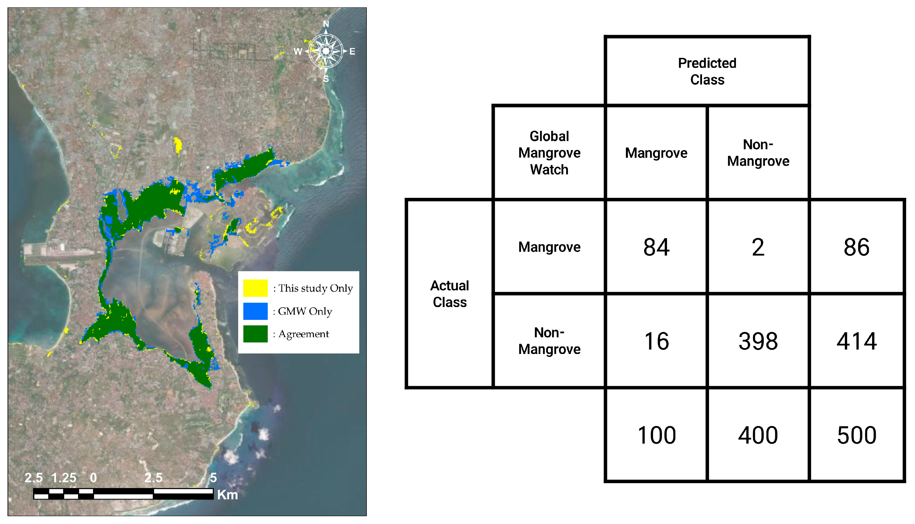
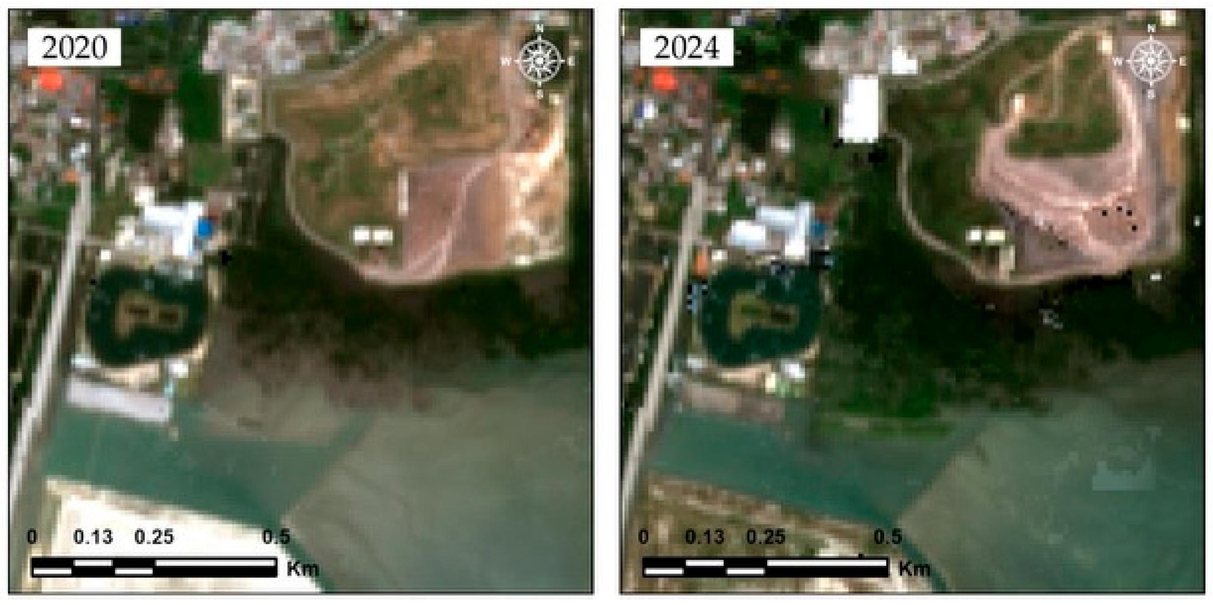
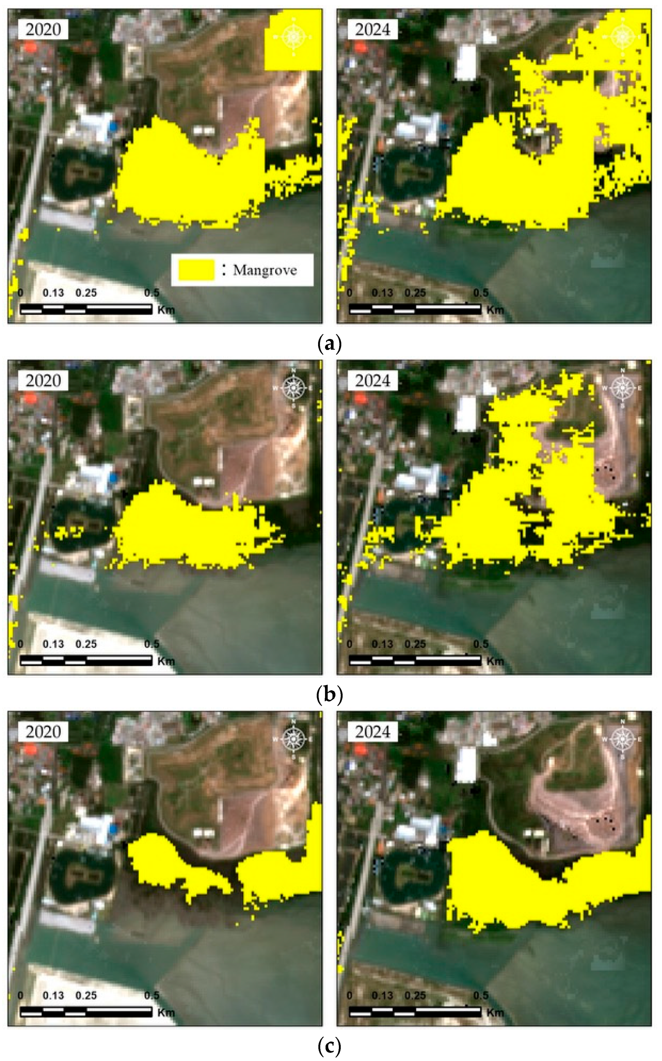
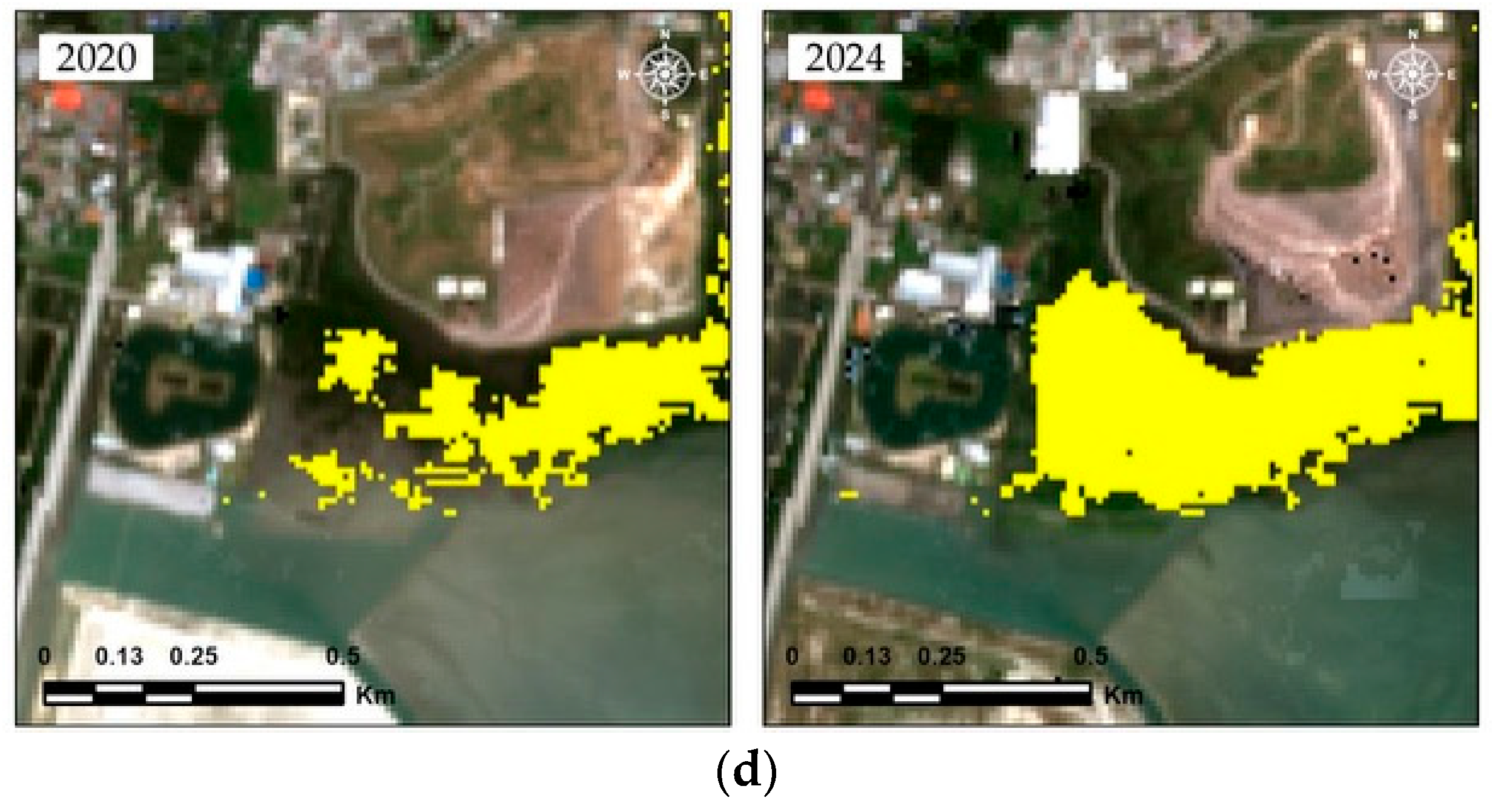
Notably, due to the lack of official mangrove label data for 2024, high-resolution satellite imagery was visually interpreted to verify the classification results. The model trained on 2020 data was successfully applied to the 2024 imagery, demonstrating its temporal transferability. This result further highlights the model’s potential for practical use in near-real-time mangrove monitoring, especially when up-to-date reference data are unavailable.
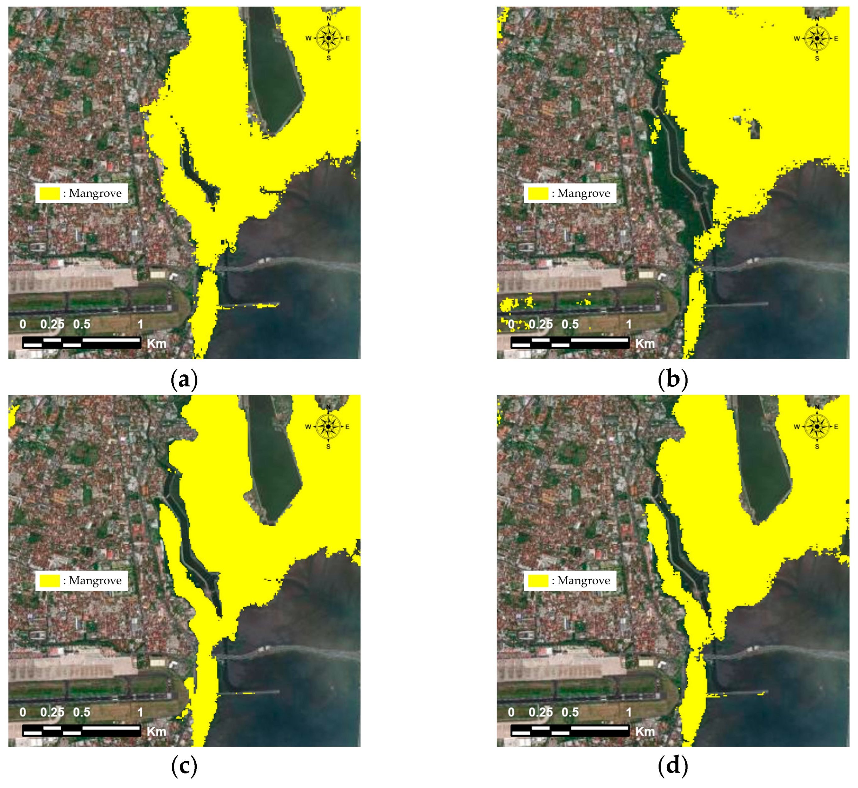
The results of this study suggest that the classification performance varies depending on how different band combinations reflect the mangrove vegetation characteristics and their interactions with other environmental factors. To better capture the complex relationship between aquatic mangrove vegetation and environmental indicators, this study integrated optical imagery with SAR data. Since optical and SAR imagery are acquired through different physical mechanisms, combining both data types allows for a more comprehensive representation of the ecological and geographical characteristics, which a single data source may fail to capture. This integration aims to overcome the limitations of single-source data and enhance classification accuracy in complex environments such as mangrove ecosystems.
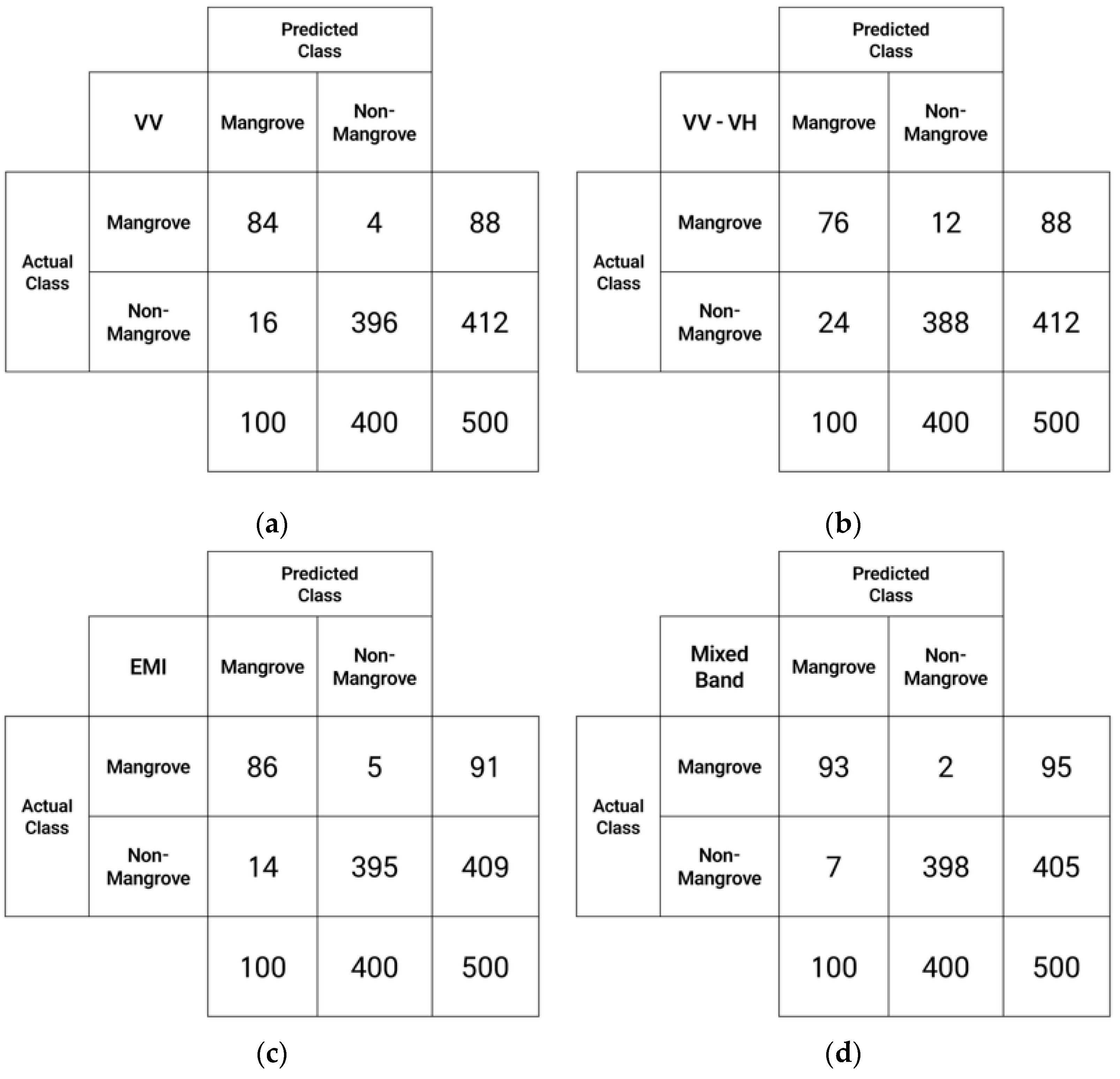
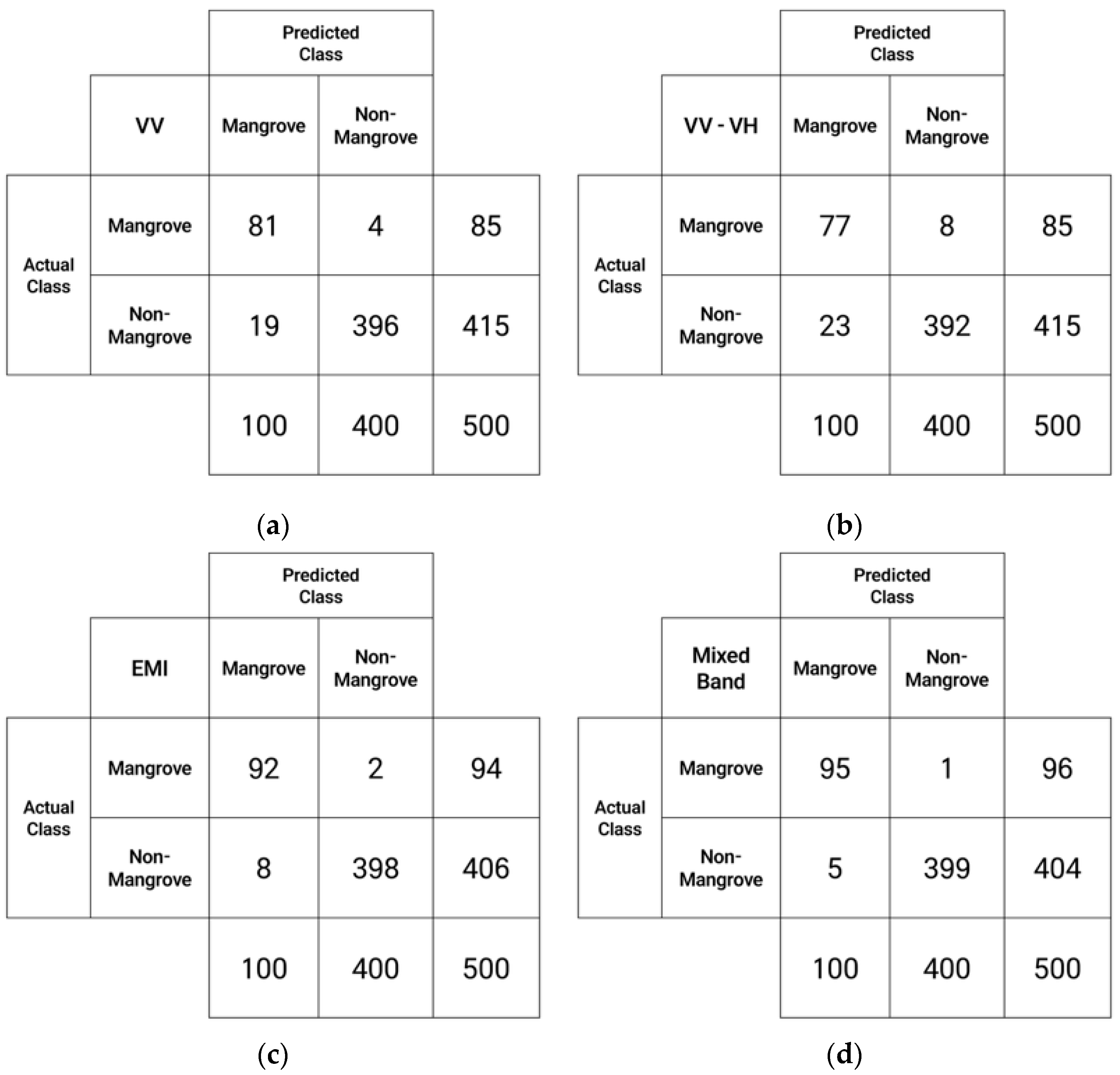
Additionally, the analysis demonstrated a significant improvement in classification accuracy when mixed bands were used compared with using optical or SAR data alone. This improvement can be attributed to the complementary characteristics of optical imagery and SAR data, which better captured the intricate properties of mangrove vegetation. The water body detection capability of SAR imagery combined with the spectral information from optical bands helped overcome the limitations of using individual data types.
However, when classification was restricted to areas with elevations below 10 m using DEM data, some actual mangrove regions were erroneously excluded, leading to omission errors. In lowland areas with similar spectral and textural characteristics, confusion still remains, especially in agricultural or high-moisture forest zones. The results suggest that the elevation criteria used in the DEM failed to fully capture the diversity and complexity of mangrove habitats, potentially restricting the accuracy of the classification data necessary for conservation and management efforts. To address these limitations, further research is needed to explore additional band combinations and develop new indices that extend beyond the current mixed band approach. In addition, strategies such as incorporating auxiliary datasets or developing region-specific post-processing rules may also be considered to better reflect the local characteristics and environmental conditions.
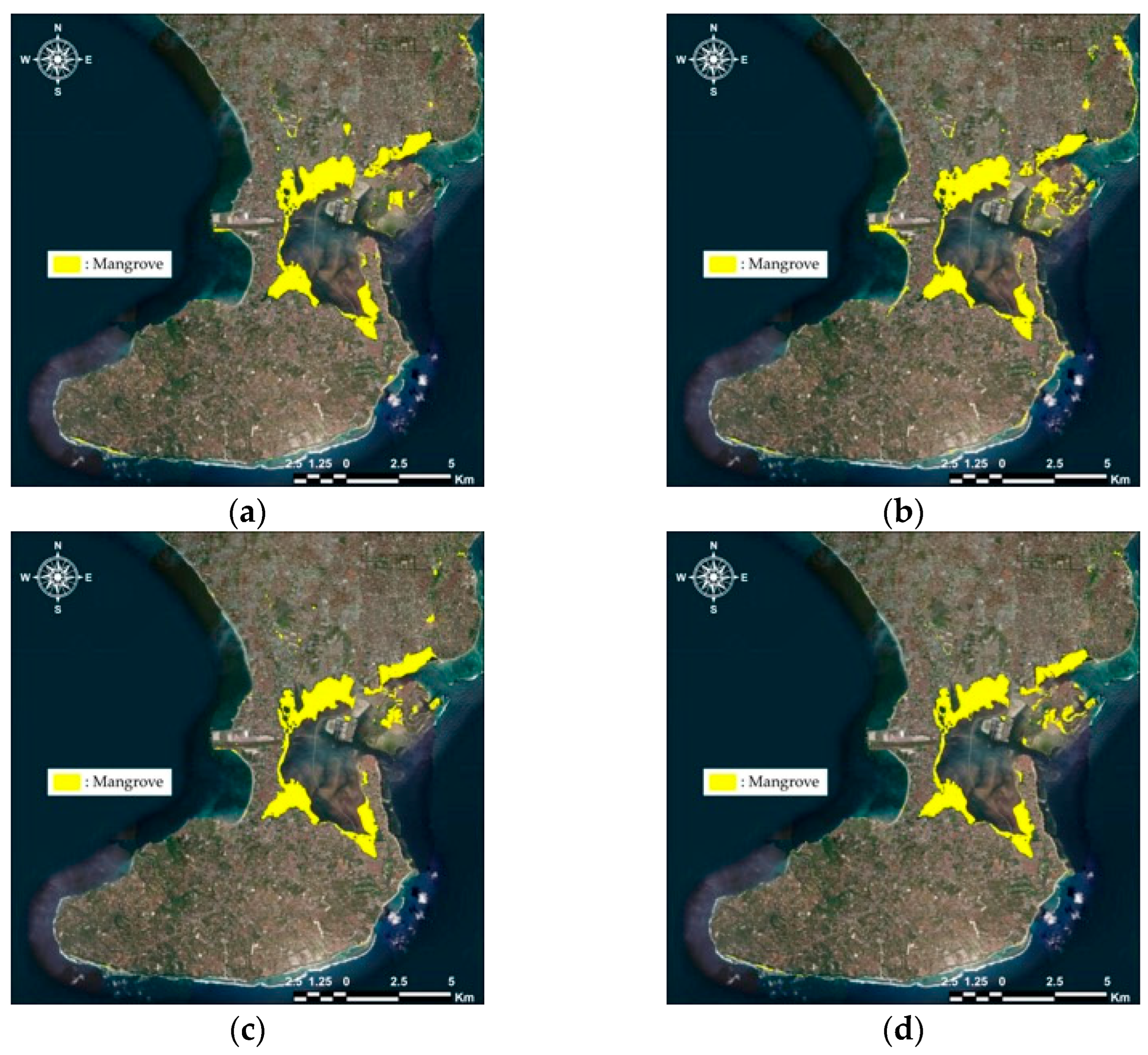
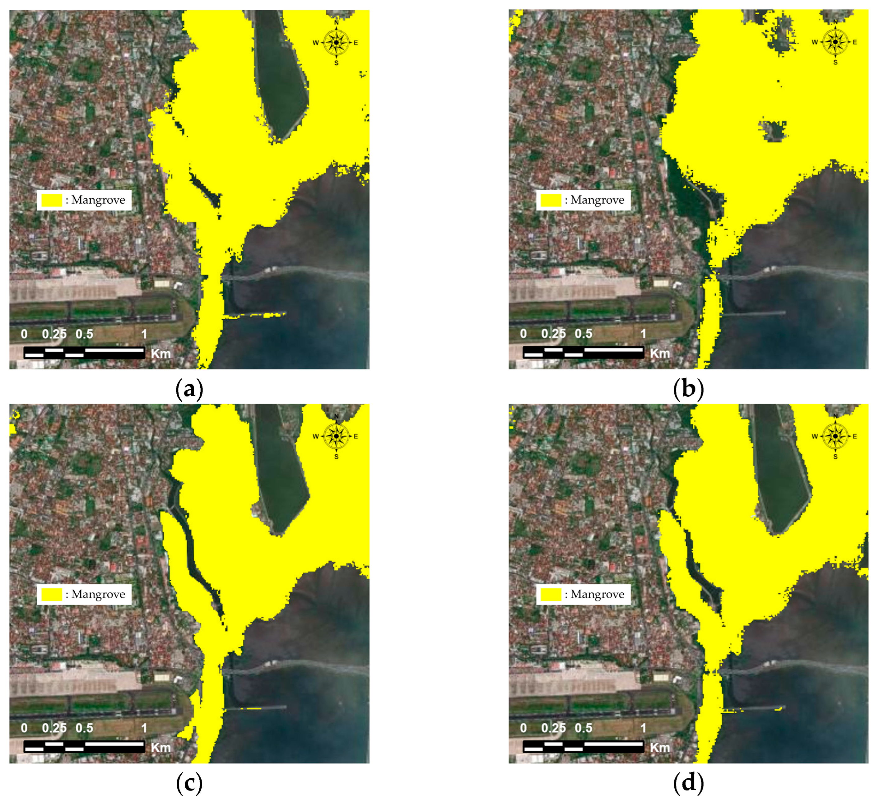
One of the primary challenges of optical imagery in tropical regions is persistent cloud cover, which limits data acquisition. In contrast, SAR data can operate independently of weather conditions, providing a significant advantage for mangrove classification in such environments. Time-series analysis revealed that VV-VH polarization-based classification provided a stable representation of mangrove area expansion, whereas VV polarization showed a minor decline in mangrove coverage. Despite this, the VV polarization still exhibited high-accuracy coverage, indicating that SAR data alone can be a reliable and effective classification method in cloud-dense conditions. The all-weather observation capability of SAR data makes it a practical alternative for mangrove classification in tropical regions.
However, overestimation was observed when classifying imagery from different years using the trained dataset. This issue is presumed to have resulted from changes in the temporal characteristics of the satellite imagery or discrepancies in the dataset. To ensure accurate time-series analysis, it is essential to develop an optimized methodology that minimizes both overestimation and underestimation by accounting for variations between datasets. To address these limitations, future studies should focus on refining the correction processes to further improve the classification accuracy.

5. Conclusions

This study adopted a hybrid approach that combined open-access SAR and optical imagery to improve the accuracy of mangrove classification and develop a model accessible to developing countries. The proposed framework prioritizes both methodological robustness and operational accessibility, enabling its deployment in areas with insufficient technological infrastructure and supporting evidence-based strategies for sustainable mangrove conservation and management in tropical regions. The U-Net-based SAR and optical imagery analysis demonstrated that the mixed band approach achieved the highest performance. While using SAR data alone resulted in lower recall values, its combination with optical data significantly improved the classification accuracy. The strong performance of the mixed band approach is likely due to the ability of SAR images to capture water-related differences between mangroves and other vegetation. These findings indicate that integrating SAR and optical data by leveraging their complementary characteristics plays a crucial role in enhancing the classification accuracy of mangrove forests. However, DEM failed to fully capture the complexity of mangrove habitats and exhibited a tendency toward overestimation in time-series classification. To mitigate these limitations, investigating novel band combinations and incorporating analysis techniques specifically optimized for time-series classification could significantly improve the classification accuracy.

Author Contributions

Conceptualization, S.K., H.K.A., C.-H.L.; Methodology, S.K., H.K.A., and C.-H.L.; Validation, S.K.; Formal analysis, S.K. and H.K.A.; Investigation, S.K.; Data curation, S.K.; Writing—original draft preparation, S.K.; Writing—review and editing, S.K. and C.-H.L.; Visualization, S.K.; Supervision, C.-H.L. All authors have read and agreed to the published version of the manuscript.

Funding

This research was funded by a National Research Foundation of Korea grant provided by the Ministry of Science and ICT (No. 2022R1C1C1008489) and a Kookmin University grant.

Data Availability Statement

The classified mangrove raster data for the Denpasar region, resulting from this study, is openly available at the Kookmin University CLIM Lab website: https://cms.kookmin.ac.kr/clim/research/researchdata1.do?mode=view&articleNo=5927333&article.offset=0&articleLimit=100, accessed on 1 March 2025.

Acknowledgments

We appreciate the cooperation of Udayana University in Bali, Indonesia, who provided the regional information and field campaign opportunity. We also appreciate Chang Bae Lee and Yong Ju Lee in the BEF lab at Kookmin University for the cooperating field dataset.

Conflicts of Interest

The authors declare no conflicts of interest.

Abbreviations

The following abbreviations are used in this manuscript:
CNNConvolutional neural network
EMIEnhanced mangrove index
ESAEuropean Space Agency
FAOFood and Agriculture Organization
GEEGoogle Earth Engine
MSIMultispectral instrument
NIRNear-infrared
SARSynthetic aperture radar
SWIRShort wavelength infrared

References

  1. Alongi, D.M. Present state and future of the world’s mangrove forests. Environ. Conserv. 2002, 29, 331–349. [Google Scholar] [CrossRef]
  2. IUCN. Environmental and Socio-Economic Value of Mangroves in Tsunami Affected Areas: Rapid Mangrove Valuation Study, Panama Village in South Eastern Coast of Sri Lanka. IUCN Report 2007. Available online: https://www.iwlearn.net/files/pdfs/IUCN%202007_Mangroves%20in%20Tsunami%20Affected%20Areas.pdf. (accessed on 14 January 2025).
  3. Sandilyan, S.; Kathiresan, K. Mangrove conservation: A global perspective. Biodivers. Conserv. 2012, 21, 3523–3542. [Google Scholar] [CrossRef]
  4. Hasan, M.; Hassan, L.; Abdullah Al, M.; Kamal, A.H.M.; Idris, M.H.; Hoque, M.Z.; Ali, A. Human intervention caused massive destruction of the second largest mangrove forest, Chakaria Sundarbans, Bangladesh. Environ. Sci. Pollut. Res. 2024, 31, 25329–25341. [Google Scholar] [CrossRef]
  5. Zeng, Y.; Friess, D.A.; Sarira, T.V.; Siman, K.; Koh, L.P. Global potential and limits of mangrove blue carbon for climate change mitigation. Curr. Biol. 2021, 31, 1737–1743. [Google Scholar] [CrossRef] [PubMed]
  6. Giesen, W.; Wulffraat, S.; Zieren, M.; Scholten, L. Mangrove Guidebook for Southeast Asia; FAO: Bangkok, Thailand, 2006; RAP Publication 2006/07. [Google Scholar]
  7. Food and Agriculture Organization of the United Nations. The World’s Mangroves 1980–2005; FAO Forestry Paper 153; FAO: Rome, Italy, 2007; ISBN 978-92-5-105856-5. [Google Scholar]
  8. Food and Agriculture Organization of the United Nations. Global Forest Resources Assessment 2020; FAO: Rome, Italy, 2020; ISBN 978-92-5-132974-0. [Google Scholar]
  9. Malik, A.; Mertz, O.; Fensholt, R. Mangrove forest decline: Consequences for livelihoods and environment in South Sulawesi. Reg. Environ. Change 2017, 17, 157–169. [Google Scholar] [CrossRef]
  10. Spalding, M.D.; Blasco, E.; Field, C.D. World Mangrove Atlas; The International Society for Mangrove Ecosystems: Okinawa, Japan, 1997. [Google Scholar]
  11. World Bank. The Economics of Large-Scale Mangrove Conservation and Restoration in Indonesia; World Bank: Washington, DC, USA, 2021. [Google Scholar]
  12. Berger, A.A. Bali Tourism; Routledge: London, UK, 2013. [Google Scholar]
  13. Bunting, P.; Rosenqvist, A.; Lucas, R.M.; Rebelo, L.-M.; Thomas, N.; Finlayson, C.M. Global Mangrove Extent Change 1996–2020: Global Mangrove Watch Version 3.0. Remote Sens. 2022, 14, 3657. [Google Scholar] [CrossRef]
  14. Xie, Y.; Rui, X.; Zou, Y.; Tang, H.; Ouyang, N. Mangrove monitoring and extraction based on multi-source remote sensing data: A deep learning method based on SAR and optical image fusion. Acta Oceanol. Sin. 2024, 43, 110–121. [Google Scholar] [CrossRef]
  15. Tran, T.V.; Reef, R.; Zhu, X.; Gunn, A. Characterising the distribution of mangroves along the southern coast of Vietnam using multi-spectral indices and a deep learning model. Sci. Total Environ. 2024, 923, 171367. [Google Scholar] [CrossRef]
  16. Kathiresan, K.; Bingham, B.L. Biology of mangroves and mangrove ecosystems. Adv. Mar. Biol. 2001, 40, 81–251. [Google Scholar]
  17. Chan, Y.K.; Koo, V. An introduction to synthetic aperture radar (SAR). Prog. Electromagn. Res. B 2008, 2, 27–60. [Google Scholar] [CrossRef]
  18. Ulaby, F.T.; Moore, R.K.; Fung, A.K. Microwave Remote Sensing: Active and Passive (Volume 1); Artech House: Norwood, MA, USA, 1981. [Google Scholar]
  19. Widantara, K.W.; Mutaqin, B.W. Multi-hazard assessment in the coastal tourism city of Denpasar, Bali, Indonesia. Nat. Hazards 2024, 120, 7105–7138. [Google Scholar] [CrossRef]
  20. World Bank. Climate Data: Historical Bali Watershed (EAP000769). Available online: https://climateknowledgeportal.worldbank.org/watershed/eap000769/climate-data-historical (accessed on 9 January 2025).
  21. Ball, M.C. Comparative Ecophysiology of Mangrove Forest and Tropical Lowland Moist Forest. In Tropical Forest Plant Ecophysiology; Mulkey, S.S., Chazdon, R.L., Smith, A.O., Eds.; Chapman and Hall: London, UK, 1996; pp. 461–469. [Google Scholar]
  22. European Space Agency. ESA World10m 2020 v100 Product Validation Report v1.1. ESA. 2020. Available online: https://worldcover2020.esa.int/data/docs/WorldCover_PVR_V1.1.pdf (accessed on 13 May 2025).
  23. Google. Sentinel-1 Algorithms | Google Earth Engine. Google for Developers. 2022. Available online: https://developers.google.com/earth-engine/guides/sentinel1 (accessed on 16 January 2025).
  24. Du, X.P.; Guo, H.D.; Fan, X.T.; Zhu, J.J.; Yan, Z.Z.; Zhan, Q. Vertical accuracy assessment of SRTM and ASTER GDEM over typical regions of China using ICESat/GLAS. Earth Sci. J. 2013, 38, 887–897. [Google Scholar]
  25. Zhang, X.; Treitz, P.M.; Chen, D.; Quan, C.; Shi, L.; Li, X. Mapping mangrove forests using multi-tidal remotely-sensed data and a decision-tree-based procedure. Int. J. Appl. Earth Obs. Geoinf. 2017, 62, 201–214. [Google Scholar] [CrossRef]
  26. Prayudha, B.; Ulumuddin, Y.I.; Siregar, V.; Agus, S.B.; Prasetyo, L.B.; Avianto, P.; Ramadhani, M.R. Enhanced mangrove index: A spectral index for discrimination understorey, nypa, and mangrove trees. MethodsX 2024, 12, 102778. [Google Scholar] [CrossRef] [PubMed]
  27. Natural Resources Canada. Radar Polarimetry. Available online: https://natural-resources.canada.ca/maps-tools-and-publications/satellite-imagery-elevation-data-and-air-photos/tutorial-fundamentals-remote-sensing/microwave-remote-sensing/radar-polarimetry/9275 (accessed on 16 January 2025).
  28. Ghasemi, M.; Karimzadeh, S.; Feizizadeh, B. Urban classification using preserved information of high dimensional textural features of Sentinel-1 images in Tabriz, Iran. Earth Sci. Inform. 2021, 14, 1745–1762. [Google Scholar] [CrossRef]
  29. Shorten, C.; Khoshgoftaar, T.M. A survey on image data augmentation for deep learning. J. Big Data 2019, 6, 60. [Google Scholar] [CrossRef]
  30. Siddique, N.; Paheding, S.; Elkin, C.P.; Devabhaktuni, V. U-net and its variants for medical image segmentation: A review of theory and applications. IEEE Access 2021, 9, 82031–82057. [Google Scholar] [CrossRef]
  31. Ronneberger, O.; Fischer, P.; Brox, T. U-net: Convolutional Networks for Biomedical Image Segmentation. In Proceedings of the Medical Image Computing and Computer-Assisted Intervention–MICCAI 2015, 18th International Conference, Munich, Germany, 5–9 October 2015, Proceedings, Part III; Springer International Publishing: Munich, Germany, 2015; pp. 234–241. [Google Scholar]
  32. Kim, J.; Lim, C.H.; Jo, H.W.; Lee, W.K. Phenological classification using deep learning and the Sentinel-2 satellite to identify priority afforestation sites in North Korea. Remote Sens. 2021, 13, 2946. [Google Scholar] [CrossRef]
  33. Cho, W.; Lim, C.H. Simplified and high accessibility approach for the rapid assessment of deforestation in developing countries: A case of Timor-Leste. Remote Sens. 2023, 15, 4636. [Google Scholar] [CrossRef]
  34. Chang, B.; Ahn, H.K.; Lim, C.H.; Cho, W. Pioneering approach for mangrove forest monitoring: Enhancing accessibility and assessment methodology in developing countries. Heliyon, 2025; in press. [Google Scholar]
  35. Koonce, B. ResNet 50. In Convolutional Neural Networks with Swift for TensorFlow: Image Recognition and Dataset Categorization; Apress: Berkeley, CA, USA, 2021; pp. 63–72. [Google Scholar]
  36. Yang, L.; Shami, A. On hyperparameter optimization of machine learning algorithms: Theory and practice. Neurocomputing 2020, 415, 295–316. [Google Scholar] [CrossRef]
  37. Olofsson, P.; Foody, G.M.; Herold, M.; Stehman, S.V.; Woodcock, C.E.; Wulder, M.A. Good practices for estimating area and assessing accuracy of land change. Remote Sens. Environ. 2014, 148, 42–57. [Google Scholar] [CrossRef]
  38. Moen, E.; Bannon, D.; Kudo, T.; Graf, W.; Covert, M.; Van Valen, D. Deep learning for cellular image analysis. Nat. Methods 2019, 16, 1233–1246. [Google Scholar] [CrossRef]
  39. Sokolova, M.; Lapalme, G. A systematic analysis of performance measures for classification tasks. Inf. Process. Manag. 2009, 45, 427–437. [Google Scholar] [CrossRef]
  40. Powers, D.M. Evaluation: From precision, recall and F-measure to ROC, informedness, markedness and correlation. arXiv 2020, arXiv:2010.16061. [Google Scholar]
  41. Saito, T.; Rehmsmeier, M. The precision-recall plot is more informative than the ROC plot when evaluating binary classifiers on imbalanced datasets. PLoS ONE 2015, 10, e0118432. [Google Scholar] [CrossRef] [PubMed]
  42. Li, J.; Chen, W.; Ying, T.; Yang, L. Double-Exposure Algorithm: A Powerful Approach to Address the Accuracy Issues of Fractional Vegetation Extraction under Shadow Conditions. Appl. Sci. 2024, 14, 7719. [Google Scholar] [CrossRef]
  43. European Space Agency (ESA). Sentinel-2|Copernicus. Available online: https://www.esa.int/Applications/Observing_the_Earth/Copernicus/Sentinel-2 (accessed on 16 January 2025).
  44. Sudiana, D.; Nisa, J.; Rizkinia, M.; Dimyati, R.D.; Anggraini, N.; Riyanto, I.; Prabuwono, A.S.; Sumantyo, J.T.S. Monitoring the Distribution of Mangrove Area Using Synthetic Aperture Radar (SAR) and Optic Remote Sensing Data Fusion Based on Deep Learning in Kotabaru Regency, Indonesia. Evergreen 2024, 11, 536–546. [Google Scholar] [CrossRef]
Figure 1. Study area in southeastern Bali, Indonesia, showing the distribution of mangrove forests in yellow and the field survey plot in red.
Remotesensing 17 01812 g001
Figure 2. Validation loss graph. (a) VV graph. (b) VV-VH graph. (c) EMI graph. (d) Mixed band graph.
Remotesensing 17 01812 g002
Figure 3. Mangrove classification results in 2020. (a) VV. (b) VV-VH. (c) EMI. (d) Mixed band.
Remotesensing 17 01812 g003
Figure 4. Mangrove classification results in 2024. (a) VV. (b) VV-VH. (c) EMI. (d) Mixed band.
Remotesensing 17 01812 g004
Figure 5. Confusion matrix for 2020. (a) VV. (b) VV-VH. (c) EMI. (d) Mixed band.
Remotesensing 17 01812 g005
Figure 6. Confusion matrix for 2024. (a) VV. (b) VV-VH. (c) EMI. (d) Mixed band.
Remotesensing 17 01812 g006
Figure 7. Spatial agreement and disagreement between this study and the Global Mangrove Watch (GMW) classification in the southeastern Bali region (left), and the confusion matrix comparing GMW-derived mangrove labels to the reference data (right). This comparison was based on the year 2020, for which GMW data were available.
Remotesensing 17 01812 g007
Figure 8. Classification results of mangroves around the channel in 2020. (a) VV. (b) VV-VH. (c) EMI. (d) Mixed band.
Remotesensing 17 01812 g008
Figure 9. The classification results of mangroves around the channel in 2024. (a) VV. (b) VV-VH. (c) EMI. (d) Mixed band.
Remotesensing 17 01812 g009
Figure 10. Mangrove change detection (2020–2024). Increase and decrease areas: (a) VV, (b) VV-VH, (c) EMI, and (d) mixed band.
Remotesensing 17 01812 g010
Figure 11. Sentinel-2 imagery of the Denpasar mangrove afforestation area (2020 vs. 2024) [43].
Remotesensing 17 01812 g011
Figure 12. Time-series comparison between 2020 and 2024. (a) VV. (b) VV-VH. (c) EMI. (d) Mixed band.
Remotesensing 17 01812 g012aRemotesensing 17 01812 g012b
Table 1. The data used in this study.
SatelliteTemporal Resolution (Day)Collection PeriodNumber of ImagesMosaic Method
Sentinel-162020-01-01~2020-12-318Percentile 75
Sentinel-252020-01-01~2020-12-3141Percentile 75
Sentinel-162024-01-01~2024-12-3159Percentile 75
Sentinel-252024-01-01~2024-12-3136Percentile 75
Table 2. The band used in this study.
SatellitePolarization and BandDerivation FormulaSource
Sentinel-1VV
VV and VHVV-VH
Sentinel-2Band 3, Band 8, and Band 11EMI 1 = (NIR − SWIR)/(GREEN + NIR)[26]
1 EMI: enhanced mangrove index.
Table 3. Number of images extracted from each satellite band.
Polarization and BandImageFeature
VV5562328
VV-VH
EMI
Mixed band
Table 4. Comparison of VV, VV-VH, EMI, and mixed bands for accuracy in 2020.
Polarization and BandAccuracyPrecisionRecallF1-Score
VV0.9598390.840.9545450.893617
VV-VH0.9280.760.8636360.808511
EMI0.9620.860.9450550.900524
Mixed band0.9820.930.9789470.953846
Table 5. Comparison of VV, VV-VH, EMI, and mixed bands for accuracy in 2024.
Polarization and BandAccuracyPrecisionRecallF1-Score
VV0.9540.810.9529410.875676
VV-VH0.9380.770.9058820.832432
EMI0.980.920.9787230.948454
Mixed band0.9880.950.9895830.969388
Table 6. GMW for accuracy in 2020.
DatasetAccuracyPrecisionRecallF1-Score
GMW 20200.9640.840.9767440.903225
Mixed band0.9820.930.9789470.953846
Table 7. Comparison of changes in mangrove area.
2020 (km2)2024 (km2)Increase (km2)Percentage Change
VV12.6712.66−0.01−0.08%
VV-VH13.2414.611.3710.37%
EMI11.7412.410.675.71%
Mixed band11.9412.110.171.42%
Disclaimer/Publisher’s Note: The statements, opinions and data contained in all publications are solely those of the individual author(s) and contributor(s) and not of MDPI and/or the editor(s). MDPI and/or the editor(s) disclaim responsibility for any injury to people or property resulting from any ideas, methods, instructions or products referred to in the content.

